Dynamics of hydrodynamically coupled Brownian harmonic oscillators in a Maxwell fluid

Abstract

Recently, many interesting features of the hydrodynamically coupled motions of the Brownian particles in a viscous fluid have been reported which are impossible for the uncoupled motions of the similar particles. However, it is expected that those physics in a viscoelastic fluid is much more interesting due to the presence of the additional frequency dependent elasticity of the medium. Thus, a theory describing the equilibrium dynamics of two hydrodynamically coupled Brownian harmonic oscillators in a viscoelastic Maxwell fluid has been derived which appears with new and impressive aspects. Initially, the response functions have been calculated and then the fluctuation-dissipation theorem has been used to calculate the correlation functions between the coloured noises present on the concerned particles placed in a Maxwell fluid due to the thermal motions of the fluid molecules. These correlation functions appear to be in a linear relationship with the delta-correlated noises in a viscous fluid. Consequently, this reduces the statistical description of a simple viscoelastic fluid to the statistical representation for an extended dynamical system subjected to delta-correlated random forces. Thereupon, the auto and cross-correlation functions in the time domain and frequency domain and the mean-square displacement functions of the particles have been calculated which are perfectly consistent with their corresponding established forms in a viscous fluid and emerge with exceptional characteristics.

I introduction

The study of the statistical properties of Brownian motion has paramount importance in Physics with varieties of applications. The random motions of colloidal particles in a viscous fluid have been studied since 1905 Einstein (1905); Von Smoluchowski (1906) and thus, well-established theory exists to describe corresponding statistical properties. Similarly, the Brownian dynamics of microscopic particles in a viscoelastic fluid are well investigated Volkov and Leonov (1996); Grimm et al. (2011); Tassieri et al. (2010); Mason and Weitz (1995), and these are entirely different from the corresponding dynamics in a purely viscous fluid. For example, at low Reynold’s number approximation and moreover, in typical experimental time scales, the inertial effect of a Brownian particle and the vorticity diffusion are negligible. Consequently, the dynamics of Brownian particles in a viscous fluid are determined only by the instantaneous forces. Thus, there is no memory Meiners and Quake (1999) and the process is known as a Markovian process. But conversely, in a viscoelastic medium, the stochastic motion of a Brownian particle is non-Markovian, even if the inertia is negligible.

Further, the hydrodynamic interaction between the moving particles in a fluid may exceptionally change the statistical description of the Brownian motion of individual particles. For instance, two hydrodynamically coupled particles in a viscous fluid in two time-independent external potentials can impose time delayed correlations between that two particles Meiners and Quake (1999); Martin et al. (2006) which is impossible for a single particle in a viscous fluid with negligible inertial effect. Again, two viscously coupled oscillators may have a frequency maximum or motional resonance effect in their mutual response function Paul et al. (2017) which is a sensitive function of the fluid viscosity. Thus, this function can be used for rheological measurements Paul et al. (2018). Such study of coupled motions of Brownian particles reveals interesting physics and definitely helps to understand the dynamics of colloidal suspensions, microscopic dynamics of proteins, dynamics of polymer solutions etc. But, as most of the fluids (emulsions, biological fluids, etc.,) are viscoelastic in nature Brust et al. (2013); Ayala et al. (2016); Doi and Edwards (1988), so the study of coupled Brownian dynamics of micro-particles in such complex fluid have fundamental importance. Understandably, there exists a strong interest in the scientific community. A viscoelastic fluid exhibits both viscous and elastic nature and thus it is typically characterized by a complex frequency dependent viscosity $\eta(\omega)$. The simplest approach developed to describe linear viscoelasticity is the Maxwell model. Further, it is improved further into a generalized form and the corresponding name of the model is Jeffreys’ model Doi and Edwards (1988); Grimm et al. (2011). It can provide the relation between stress and shear-rate in linear viscoelastic fluids which can be used to evaluate trajectories of Brownian particles in such medium.

Although some statistical properties of the coupled dynamics in a complex fluid have been used for the purpose of rheological measurements Crocker et al. (2000); Crocker and Hoffman (2007), the coupled dynamics of Brownian particles in such fluid is still not studied elaborately which may disclose several interesting physics and can be used to measure rheological parameters more precisely.

This work theoretically describes the dynamics of two hydrodynamically coupled Brownian particles bound in two harmonic oscillator potentials in a Maxwell fluid with single relaxation time. The response functions of the particles under external perturbations have been calculated and it has been shown that these functions are entirely different in a Maxwell fluid as compared to the reported forms in a viscous fluid Paul et al. (2017, 2018). Furthermore, the fluctuation-dissipation theorem (FDT) has been used to calculate the correlations between stochastic noises on the two particles in the study. It has been shown that the noise correlations in Maxwell fluid are linearly related to the correlations of noises in a viscous fluid by a function. Thus, such problem of coupled Brownian motion with the simplest viscoelastic liquid can be reduced to the statistical description of an extended dynamical system subjected to a delta-correlated random force. This method is reported for a single particle in Maxwell fluid with one relaxation time Volkov and Leonov (1996). Then the position correlation functions in the frequency domain and in the time domain and the mean-square displacement functions of the particles have also been calculated and studied. It has been shown in addition that the correlation between two particles in Maxwell fluid is time-delayed, but the time delay linearly depends on the Maxwell relaxation time $\tau$, which represents the crossover time scale of the fluid from elastic to viscous behaviour. Consequently, $\tau\rightarrow 0$ represent the statistical description of the particles motion in the viscous fluid. Besides, if the particles are significantly separated and if the hydrodynamic coupling is negligible then they behave like uncoupled particles and show corresponding statistical properties. The zero stiffnesses consideration of the bounding potentials converges the dynamics to the free but hydrodynamically coupled dynamics of the concerned particles.

II Theory

The one-dimensional translational motion of two hydrodynamically coupled identical colloidal spheres bound in two different harmonic oscillator potential wells in Maxwell fluid with a single relaxation time $\tau$ can be described by the set of equations Gardiner (1984); Volkov and Leonov (1996)

$$m\ddot{x}_{1} =F_{1}-k_{1}x_{1}+\varepsilon(-k_{2}x_{2}+f_{2})+f_{1}$$ (1)

$$m\ddot{x}_{2} =F_{2}-k_{2}x_{2}+\varepsilon(-k_{1}x_{1}+f_{1})+f_{2}$$ (2)

where, $F_{1}$ and $F_{2}$ are the relaxed frictions which are given by

$$\tau\frac{dF_{1}}{dt}+F_{1} =-\zeta_{0}\dot{x}_{1}$$ (3)

$$\tau\frac{dF_{2}}{dt}+F_{2} =-\zeta_{0}\dot{x}_{2}$$ (4)

$x_{1}$, $x_{2}$ are the positions of the first and second particles respectively w.r.t. their corresponding potential minimums; $k_{1}$ and $k_{2}$ are the stiffnesses of the first and second harmonic oscillators respectively; $\varepsilon=\frac{3a_{0}}{2d}-\left(\frac{a_{0}}{d}\right)^{3}$ is the hydrodynamic coupling coefficient.; $a_{0}$ is the radius of each of the particles and $d$ is the center to center separation between these two particles; $\zeta_{0}=6\pi\eta_{0}a_{0}$ is the drag coefficient at zero frequency; $\eta_{0}$ is the zero frequency viscosity of the fluid; $m$ is the mass of each of the particles. The particles are far apart from each other so that $d$ can be assumed to be constant in time. $f_{1}$ and $f_{2}$ are the perturbations on first and second particles respectively, which can be due to the random motions of the surrounding molecules of the fluid or due to some external disturbance. In low Reynolds number regime, the effect of inertia dies out in a time scale $\tau^{*}=m/\zeta_{0}$ which is known as the momentum relaxation time scale. $\tau^{*}$ is of the order of $\sim 10^{-6}$ sec which is much lower than the typical experimental time scales. Hence, the inertial effect is negligible and the terms in the left hand side of Equs. (1) and (2) can be approximated to zero and thus can be written as

$$0=F_{1}-k_{1}x_{1}+\varepsilon(-k_{2}x_{2}+f_{2})+f_{1}$$ (5)

$$0=F_{2}-k_{2}x_{2}+\varepsilon(-k_{1}x_{1}+f_{1})+f_{2}$$ (6)

The systematic viscoelastic drag forces $F_{i}$ ($i=1,\,2$) tend to $-\zeta_{0}\dot{x}_{i}$ as the relaxation time $\tau$ converges to zero, which is clear from the set of Equs. (3),(4). This is the familiar expression of the Stokes drag force in viscous fluid. Now, the Equs. (3) and (4) can be easily solved to yield the expressions for the drags on the spheres in Maxwell fluid in terms of the initial forces $F_{i}^{0}$ as

$$F_{i}(t)=F_{i}^{0}e^{-(t-t_{0})/\tau}-\intop_{t_{0}}^{t}\zeta(t-s)\dot{x}_{i}(s)ds$$ (7)

where the memory kernel $\zeta(t)=\frac{\zeta_{0}}{\tau}e^{-t/\tau}$. It can be assumed that the initial time was $-\infty$ and then $F_{i}^{0}=0$. On this assumption, the expressions for the drags on the spheres are

$$F_{i}(t)=-\frac{\zeta_{0}}{\tau}\intop_{-\infty}^{t}e^{-(t-s)}\dot{x}_{i}(s)ds$$ (8)

The memory kernel represents the time-dependent viscoelastic resistance, to which a spherical particle moving in a stationary Maxwell fluid is subjected. The relation between the complex viscosity and the complex viscoelastic resistance is $\eta(\omega)=\frac{1}{6\pi a_{0}}\zeta(\omega)$ where $\zeta(\omega)$ is the one-sided Fourier transformation of $\zeta(t)$ which is defined as $\zeta(\omega):=\int\zeta(t)e^{-i\omega t}dt$. Hence, $\eta(\omega)=\frac{\eta_{0}}{1+i\omega\tau}$. Now, Equs. (5), (3) and (6), (4) can be coupled to get

$$0=-(\zeta_{0}+k_{1}\tau)\dot{x}_{1}-\varepsilon\tau k_{2}\dot{x}_{2}-k_{1}x_{1}-\varepsilon k_{2}x_{2}$$

$$+\varepsilon(f_{2}+\tau\dot{f}_{2})+(f_{1}+\tau\dot{f}_{1})$$ (9)

$$0=-(\zeta_{0}+k_{2}\tau)\dot{x}_{2}-\varepsilon\tau k_{1}\dot{x}_{1}-k_{2}x_{2}-\varepsilon k_{1}x_{1}$$

$$+\varepsilon(f_{1}+\tau\dot{f}_{1})+(f_{2}+\tau\dot{f}_{2})$$ (10)

and then, Equs. (9) and (10) can be Fourier transformed which then can be written in matrix form as

$$\boldsymbol{0=-}\boldsymbol{A}(\omega)\cdot\boldsymbol{x}(\omega)+\boldsymbol{M}(\omega)\cdot\boldsymbol{f}(\omega)$$ (11)

$$\boldsymbol{A}(\omega)=\begin{pmatrix}-i\omega\gamma_{1}-k_{1}&-\varepsilon k_{2}(i\omega\tau-1)\\ -\varepsilon k_{1}(i\omega\tau-1)&-i\omega\gamma_{2}-k_{2}\end{pmatrix}$$

$$\boldsymbol{M}(\omega)=(1-i\omega\tau)\begin{pmatrix}1&\varepsilon\\ \varepsilon&1\end{pmatrix}$$

$$\boldsymbol{x}(\omega)=\begin{pmatrix}x_{1}(\omega)\\ x_{2}(\omega)\end{pmatrix},\,\boldsymbol{f}(\omega)=\begin{pmatrix}f_{1}(\omega)\\ f_{2}(\omega)\end{pmatrix}$$

where, $\gamma_{i}=\zeta_{0}+k_{i}\tau$. Therefore, Eq. (11) can be written as

$$\boldsymbol{x}(\omega)=\boldsymbol{A}^{-1}(\omega)\cdot\boldsymbol{M}(\omega)\cdot\boldsymbol{f}(\omega)=\boldsymbol{\chi}(\omega)\cdot\boldsymbol{f}(\omega)$$ (12)

where, $\boldsymbol{\mathbb{\chi}}(\omega)=\boldsymbol{A}^{-1}(\omega)\cdot\boldsymbol{M}(\omega)$ is the response matrix of the two-particle system. The bold-face notation has been used to represent both matrices and vectors. The response matrix is given by

$$\boldsymbol{\mathbb{\chi}}(\omega)=\frac{\left\{(\alpha\omega^{2}+\nu)+i\omega\beta\right\}(-i\omega\tau+1)}{(\alpha\omega^{2}+\nu)^{2}+(\omega\beta)^{2}}\times$$

$$\begin{pmatrix}k_{2}(1-\varepsilon^{2})-i\omega(\gamma_{2}-\varepsilon^{2}k_{2}\tau)&-\varepsilon i\omega\zeta_{0}\\ -\varepsilon i\omega\zeta_{0}&k_{1}(1-\varepsilon^{2})-i\omega(\gamma_{1}-\varepsilon^{2}k_{1}\tau)\end{pmatrix}$$

$$=\begin{pmatrix}\chi_{11}(\omega)&\chi_{12}(\omega)\\ \chi_{21}(\omega)&\chi_{22}(\omega)\end{pmatrix}$$ (13)

where,

$$\alpha=\varepsilon^{2}\tau^{2}k_{1}k_{2}-\gamma_{1}\gamma_{2}$$

$$\beta=\gamma_{1}k_{2}+\gamma_{2}k_{1}-2\varepsilon^{2}k_{1}k_{2}\tau$$

$$\nu=k_{1}k_{2}(1-\varepsilon^{2})$$

$\chi_{ij}(\omega)\,(i\,j=1,\,2)$ are the components of the symmetric matrix$\boldsymbol{\chi}(\omega)$ ($\chi_{12}(\omega)=\chi_{21}(\omega)$). From Eq. (13) one can calculate the amplitude and the phase of the mutual response function of the system which indicates the response of one particle due to the application of unit force on the other. The expressions are given by

$$\bigl{|}\chi_{12}(\omega)\bigr{|}=\omega\varepsilon\zeta_{0}\times\\ \frac{\sqrt{\bigl{\{}(\beta-\nu\tau)-\alpha\tau\omega^{2}\bigr{\}}^{2}\omega^{2}+\bigl{\{}\nu+(\alpha+\beta\tau)\omega^{2}\bigr{\}}^{2}}}{(\alpha\omega^{2}+\nu)^{2}+(\omega\beta)^{2}}$$ (14)

$$\Phi(\omega)=\tan^{-1}\Biggl{[}\frac{\nu+(\alpha+\beta\tau)\omega^{2}}{\alpha\tau\omega^{2}+(\nu\tau-\beta)\omega}\Biggr{]}$$ (15)

In Fig. 1 the amplitude $\bigl{|}\chi_{12}(\omega)\bigr{|}$ and the phase $\Phi(\omega)$ of the mutual response function $\chi_{12}(\omega)$ have been plotted w.r.t angular frequency $\omega$. At $\tau=0$, the medium is purely viscous and at a particular frequency of the external drive, the probe particle absorbs maximum energy and the response is thus maximum. At that frequency, the phase is zero Paul et al. (2017). This frequency in viscous medium is viscosity dependent and thus it can be used to measure the viscosity of the surrounding medium Paul et al. (2018). But if $\tau>0$, the nature of the coupling changes entirely. The peak in the amplitude decreases with the increase of $\tau$ and after certain value of $\tau$ the peak vanishes. It is also clear from the figure that the peak frequency decreases with the increase of $\tau$ but on the other hand the zero-crossing frequency in the phase plot increases. The plots can be described from Equs. (14) and (15) which are very much different from the reported functions in a viscous medium.

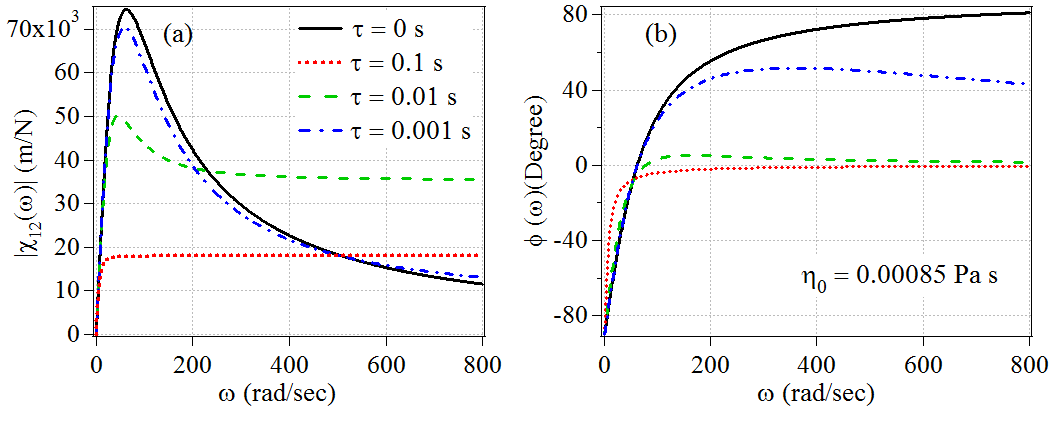
Figure 1: The plot of (a) amplitude $|\chi_{12}(\omega)|$ and (b) phase $\phi(\omega)$ of the mutual response function $\chi_{12}(\omega)$ as a function of the angular frequency $\omega$ for different values of $\tau$. Black line, blue dot-dashes, green dashes and red dots are for $\tau=0$ s, $0.001$ s, $0.01$ s and $0.1$ s respectively. The zero frequency viscosity is kept constant at $\eta_{0}=0.00085$ Pa s. Other parameters have been taken as $a_{0}=1\,\mu m$, $d=10a_{0}$, $k_{1}=k_{2}=1\,\mu N/m$ which are experimentally relevant.

II.1 Calculation for the noise correlation matrix:

It can be assumed that the perturbation $\boldsymbol{f}(\omega)$ in Eq. (12) on the system is due to the random thermal motions of the molecules of the surrounding fluid. The random perturbation (noise) is the manifestation of a large number of equally strong, independent impulses which change direction rapidly. Therefore, according to the central limit theorem, the distribution of the noise will be Gaussian with zero mean ($\langle\boldsymbol{f}(\omega)\rangle=\boldsymbol{0}$). Now, the inherent elasticity of the fluid enables the system to store energy and thus the noise becomes correlated. Here, the attempt is to find out the correlation. In equilibrium, the well known fluctuation-dissipation theorem (FDT) relates the correlation matrix $\langle\boldsymbol{x}(\omega)\boldsymbol{x}^{\dagger}(\omega)\rangle$ of the system to the deterministic response matrix in the following form Kubo (1966)

$$\langle\boldsymbol{x}(\omega)\boldsymbol{x}^{\dagger}(\omega)\rangle =\frac{2k_{B}T}{\omega}\Im[\boldsymbol{\mathbb{\chi}}(\omega)]$$ (16)

where, $\Im[\boldsymbol{\mathbb{\chi}}(\omega)]$ is the imaginary part of the response function. The position correlation matrix of the system of particles can be written as

$$\langle\boldsymbol{x}(\omega)\boldsymbol{x}^{\dagger}(\omega)\rangle=\mathbb{\boldsymbol{\chi}}(\omega)\cdot\langle\boldsymbol{f}(\omega)\boldsymbol{f}^{\dagger}(\omega)\rangle\cdot\mathbb{\boldsymbol{\chi}}^{\dagger}(\omega)$$ (17)

where, Eq. (12) has been used. Further, the imaginary part of the response function can be written as

$$\Im[\boldsymbol{\mathbb{\chi}}(\omega)]=\frac{1}{2i}(\boldsymbol{\mathbb{\chi}}(\omega)-\boldsymbol{\mathbb{\chi}}^{*}(\omega))=\frac{1}{2i}(\mathbb{\boldsymbol{\chi}}(\omega)-\mathbb{\boldsymbol{\chi}}^{\dagger}(\omega))$$ (18)

Since, $\boldsymbol{\mathbb{\chi}}(\omega)$ is symmetric so $\boldsymbol{\chi}^{*}(\omega)=\mathbb{\boldsymbol{\chi}}^{\dagger}(\omega)$. Hence, one can write using Equs. (16), (17) and (18)

$$\mathbb{\boldsymbol{\chi}}(\omega)\cdot\langle\boldsymbol{f}(\omega)\boldsymbol{f}^{\dagger}(\omega)\rangle\cdot\mathbb{\boldsymbol{\chi}}^{\dagger}(\omega)=\frac{2k_{B}T}{2i\omega}(\boldsymbol{\mathbb{\chi}}(\omega)-\mathbb{\boldsymbol{\chi}}^{\dagger}(\omega))$$ (19)

Thus,

$$\langle\boldsymbol{f}(\omega)\boldsymbol{f}^{\dagger}(\omega)\rangle = \frac{k_{B}T}{i\omega}\mathbb{\boldsymbol{\chi}}^{-1}(\omega)\cdot(\mathbb{\boldsymbol{\chi}}(\omega)-\mathbb{\boldsymbol{\chi}}^{\dagger}(\omega))\cdot(\boldsymbol{\chi}^{\dagger}(\omega))^{-1}$$ (20)

$$= \frac{k_{B}T}{i\omega}\biggl{(}(\boldsymbol{\chi}^{\dagger}(\omega))^{-1}-\mathbb{\boldsymbol{\chi}}^{-1}(\omega)\biggr{)}$$

Now, the response function can be written as

$$\mathbb{\boldsymbol{\chi}}(\omega)=(1-i\omega\tau)\boldsymbol{A}^{-1}(\omega)\cdot\boldsymbol{M}_{1}$$

where, $\boldsymbol{M}(\omega)=(1-i\omega\tau)\boldsymbol{M}_{1}$. Again,

$$\chi(\omega)=\frac{(1-i\omega\tau)}{\det(\boldsymbol{A}(\omega))}\widetilde{\mathbb{\boldsymbol{\chi}}}(\omega)=\frac{(1-i\omega\tau)}{\det(\boldsymbol{A}(\omega))}\begin{pmatrix}\widetilde{\chi}_{11}(\omega)&\widetilde{\chi}_{12}(\omega)\\ \widetilde{\chi}_{21}(\omega)&\widetilde{\chi}_{22}(\omega)\end{pmatrix}$$

where, $\widetilde{\mathbb{\boldsymbol{\chi}}}(\omega)=adj(\boldsymbol{A}(\omega))\cdot\boldsymbol{M}_{1}$ and the corresponding components are given by

$$\widetilde{\chi}_{11}(\omega)=k_{2}(1-\varepsilon^{2})+i\omega(\varepsilon^{2}k_{2}\tau-\gamma_{2})$$ (21)

$$\widetilde{\chi}_{22}(\omega)=k_{1}(1-\varepsilon^{2})+i\omega(\varepsilon^{2}k_{1}\tau-\gamma_{1})$$ (22)

$$\widetilde{\chi}_{12}(\omega)=\widetilde{\chi}_{21}(\omega)=-i\omega\varepsilon\zeta_{0}$$ (23)

Therefore,

$$\boldsymbol{\mathbb{\chi}}^{-1}(\omega)=\frac{\det(\boldsymbol{A}(\omega))}{(1-i\omega\tau)}\times$$

$$\frac{1}{\det(\boldsymbol{A}(\omega))\det(\boldsymbol{M}_{1})}\begin{pmatrix}\widetilde{\chi}_{22}(\omega)&-\widetilde{\chi}_{12}(\omega)\\ -\widetilde{\chi}_{21}(\omega)&\widetilde{\chi}_{11}(\omega)\end{pmatrix}$$ (24)

$$\boldsymbol{\mathbb{\chi}}^{-1}(\omega)=\frac{1}{(1-i\omega\tau)(1-\varepsilon^{2})}\begin{pmatrix}\widetilde{\chi}_{22}(\omega)&-\widetilde{\chi}_{12}(\omega)\\ -\widetilde{\chi}_{21}(\omega)&\widetilde{\chi}_{11}(\omega)\end{pmatrix}$$ (25)

Similarly,

$$(\mathbb{\boldsymbol{\chi}}^{\dagger}(\omega))^{-1}=\frac{1}{(1+i\omega\tau)(1-\varepsilon^{2})}\begin{pmatrix}\widetilde{\chi}_{22}^{*}(\omega)&-\widetilde{\chi}_{12}^{*}(\omega)\\ -\widetilde{\chi}_{21}^{*}(\omega)&\widetilde{\chi}_{11}^{*}(\omega)\end{pmatrix}$$ (26)

Using above Equs. (20)-(26) one can obtain the correlation

$$\langle\boldsymbol{f}(\omega)\boldsymbol{f}^{\dagger}(\omega)\rangle=\frac{2k_{B}T\zeta_{0}}{1+(\omega\tau)^{2}}\begin{pmatrix}1&\varepsilon\\ \varepsilon&1\end{pmatrix}^{-1}$$ (27)

The corresponding correlation matrix in time domain is a result of the Fourier transform of Eq. (27) and is given by

$$\langle\boldsymbol{f}(t)\boldsymbol{f}^{\dagger}(0)\rangle=\frac{k_{B}T\zeta_{0}}{\tau}e^{-|t|/\tau}\begin{pmatrix}1&\varepsilon\\ \varepsilon&1\end{pmatrix}^{-1}$$ (28)

This means, the random forces $\boldsymbol{f}(t)$ acting on the system of particles in Maxwell fluid are exponentially correlated and thus Markovian. As $\tau$ approaches zero, the correlation converges to the familiar form in a viscous medium which is given by

$$\langle\boldsymbol{f}(t)\boldsymbol{f}^{\dagger}(0)\rangle=2k_{B}T\zeta_{0}\delta(t)\begin{pmatrix}1&\varepsilon\\ \varepsilon&1\end{pmatrix}^{-1}$$ (29)

The Markovian random forces can be represented as the solution of a stochastic differential equation

$$\tau\frac{d}{dt}\boldsymbol{f}(t)+\boldsymbol{f}(t)=\boldsymbol{\xi}(t)$$ (30)

where $\boldsymbol{\xi}(t)$ are random forces with correlation

$$\langle\boldsymbol{\xi}(t)\boldsymbol{\xi}^{\dagger}(0)\rangle=2k_{B}T\zeta_{0}\delta(t)\begin{pmatrix}1&\varepsilon\\ \varepsilon&1\end{pmatrix}^{-1}$$ (31)

II.2 Calculation for the correlations and the mean-square displacements of the particles:

From Eq. (30), it can be obtained that the generalized random force $\boldsymbol{\xi}(t)$ is related to the Markovian random force $\boldsymbol{f}(t)$ by the relation

$$\boldsymbol{\xi}(\omega)=(1-i\omega\tau)\boldsymbol{f}(\omega)$$ (32)

Eq. (32) can be substituted into Eq. (12) and one can obtain,

$$\boldsymbol{x}(\omega)=\frac{1}{(1-i\omega\tau)}\boldsymbol{\chi}(\omega)\cdot\boldsymbol{\xi}(\omega)=\boldsymbol{\chi}_{g}(\omega)\cdot\boldsymbol{\xi}(\omega)$$

Hence, the response $\boldsymbol{x}(\omega)$ and the generalized random force is related linearly by the generalized susceptibility $\boldsymbol{\chi}_{g}(\omega)=\frac{1}{(1-i\omega\tau)}\boldsymbol{\chi}(\omega)$ of the system. Thus, in equilibrium, the position correlation matrix of the system due to the thermal motions of the particles can be obtained in terms of the generalized susceptibility $\boldsymbol{\chi}_{g}(\omega)$ as

$$\boldsymbol{C}(\omega) =\frac{2k_{B}T}{\omega}\Im[\boldsymbol{\mathbb{\chi}}_{g}(\omega)]$$ (33)

$$\begin{pmatrix}C_{11}(\omega)&C_{12}(\omega)\\ C_{21}(\omega)&C_{22}(\omega)\end{pmatrix} =\frac{2k_{B}T}{\omega}\Im\Biggl{[}\frac{1}{(1-i\omega\tau)}\begin{pmatrix}\chi_{11}(\omega)&\chi_{12}(\omega)\\ \chi_{21}(\omega)&\chi_{22}(\omega)\end{pmatrix}\Biggr{]}$$ (34)

$\boldsymbol{C}(\omega)$ is the correlation matrix in frequency domain and $C_{ij}(\omega)\,(i\,j=1,\,2)$ are the corresponding components, $k_{B}$ is the Boltzmann constant and $T$ is the temperature. Now, from Equs. (34) and (13) one can get

$$C_{11}(\omega)=\frac{2k_{B}T}{(\alpha\omega^{2}+\nu)^{2}+(\omega\beta)^{2}}\times$$

$$\biggl{[}\bigl{\{}\alpha(\varepsilon^{2}k_{2}\tau-\gamma_{2})\bigr{\}}\omega^{2}+$$

$$\bigl{\{}\beta k_{2}(1-\varepsilon^{2})+\nu(\varepsilon^{2}k_{2}\tau-\gamma_{2})\bigr{\}}\biggr{]}$$ (35)

$$C_{22}(\omega)=\frac{2k_{B}T}{(\alpha\omega^{2}+\nu)^{2}+(\omega\beta)^{2}}\times$$

$$\biggl{[}\bigl{\{}\alpha(\varepsilon^{2}k_{1}\tau-\gamma_{1})\bigr{\}}\omega^{2}+$$

$$\bigl{\{}\beta k_{1}(1-\varepsilon^{2})+\nu(\varepsilon^{2}k_{1}\tau-\gamma_{1})\bigr{\}}\biggr{]}$$ (36)

$$C_{12}(\omega)=C_{21}(\omega)=-\frac{2k_{B}T}{(\alpha\omega^{2}+\nu)^{2}+(\omega\beta)^{2}}\times$$

$$\biggl{[}\varepsilon\zeta_{0}\bigl{\{}\alpha\omega^{2}+\nu\bigr{\}}\biggr{]}$$ (37)

Now, the position correlation functions of the particles in the time domain can be obtained by Fourier transforming Equs. (35), (36) and (37). Which yields,

$$C_{ii}(t)=\left<x_{i}(t)x_{i}(0)\right>=$$

$$\frac{1}{\nu_{1}}\Biggl{[}\frac{a_{ii}-\frac{b_{ii}}{4}(c-\nu_{1})^{2}}{\biggl{\{}\left(\frac{c-\nu_{1}}{2}\right)^{2}+\left(\frac{c-\nu_{1}}{2}\right)c+\omega_{0}\biggr{\}}}\exp\biggl{(}-\left(\frac{c-\nu_{1}}{2}\right)t\biggr{)}$$

$$+\frac{\frac{b_{ii}}{4}(c+\nu_{1})^{2}-a_{ii}}{\biggl{\{}\left(\frac{c+\nu_{1}}{2}\right)^{2}+\left(\frac{c+\nu_{1}}{2}\right)c+\omega_{0}\biggr{\}}}\exp\biggl{(}-\left(\frac{c+\nu_{1}}{2}\right)t\biggr{)}\Biggr{]}$$ (38)

$$C_{ij}(t)=\left<x_{i}(t)x_{j}(0)\right>=$$

$$\frac{1}{\nu_{1}}\Biggl{[}\frac{a_{ij}-\frac{b_{ij}}{4}(c-\nu_{1})^{2}}{\biggl{\{}\left(\frac{c-\nu_{1}}{2}\right)^{2}+\left(\frac{c-\nu_{1}}{2}\right)c+\omega_{0}\biggr{\}}}\exp\biggl{(}-\left(\frac{c-\nu_{1}}{2}\right)t\biggr{)}$$

$$+\frac{\frac{b_{ij}}{4}(c+\nu_{1})^{2}-a_{ij}}{\biggl{\{}\left(\frac{c+\nu_{1}}{2}\right)^{2}+\left(\frac{c+\nu_{1}}{2}\right)c+\omega_{0}\biggr{\}}}\exp\biggl{(}-\left(\frac{c+\nu_{1}}{2}\right)t\biggr{)}\Biggr{]}$$ (39)

$$C_{ij}(t)=C_{ji}(t)$$ (40)

where, $a_{ii}=\frac{2k_{B}T}{\alpha^{2}}\bigl{\{}\beta k_{j}(1-\varepsilon^{2})+\nu(\varepsilon^{2}k_{j}\tau-\gamma_{j})\bigr{\}}$, $b_{ii}=\frac{2k_{B}T}{\alpha^{2}}\bigl{\{}\alpha(\varepsilon^{2}k_{j}\tau-\gamma_{j})\bigr{\}}$, $a_{ij}=-\frac{2k_{B}T}{\alpha^{2}}\varepsilon\zeta_{0}\nu$, $b_{ij}=-\frac{2k_{B}T}{\alpha}\varepsilon\zeta_{0}$ $\omega_{0}=-\frac{\nu}{\alpha}$, $c=-\frac{\beta}{\alpha}$ and $\nu_{1}=\sqrt{c^{2}-4\omega_{0}}$. $i,\,j=1,\,2;\,i\neq j$. The mean-square displacement functions (MSD) is related to the correlation functions as

$$\left\langle\Delta x_{i}^{2}(t)\right\rangle=2\left[\left\langle x_{i}^{2}(0)\right\rangle-\left\langle x_{i}(t)x_{i}(0)\right\rangle\right]$$

$$=\frac{2}{\nu_{1}}\Biggl{[}\frac{a_{ii}-\frac{b_{ii}}{4}(c-\nu_{1})^{2}}{\biggl{\{}\left(\frac{c-\nu_{1}}{2}\right)^{2}+\left(\frac{c-\nu_{1}}{2}\right)c+\omega_{0}\biggr{\}}}\Biggl{(}1-\exp\biggl{(}-\left(\frac{c-\nu_{1}}{2}\right)t\biggr{)}\Biggr{)}$$

$$+\frac{\frac{b_{ii}}{4}(c+\nu_{1})^{2}-a_{ii}}{\biggl{\{}\left(\frac{c+\nu_{1}}{2}\right)^{2}+\left(\frac{c+\nu_{1}}{2}\right)c+\omega_{0}\biggr{\}}}\Biggl{(}1-\exp\biggl{(}-\left(\frac{c+\nu_{1}}{2}\right)t\biggr{)}\Biggr{)}\Biggr{]}$$ (41)

In Fig. 2, the cross-correlation functions for different $\tau$ has been plotted. With the increase of $\tau$, the maximum correlation between the particles appear in larger time-lag which increases linearly with $\tau$ and the corresponding correlation decreases exponentially. It has been shown in Fig. 3.

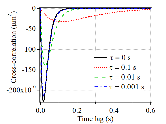
Figure 2: The plot of the cross-correlation function with respect to time-lag. The parameters are same as described in Fig. 1. Black line, blue dot-dashes, green dashes and red dots represent $\tau=0$ s, $0.001$ s, $0.01$ s and $0.1$ s respectively.

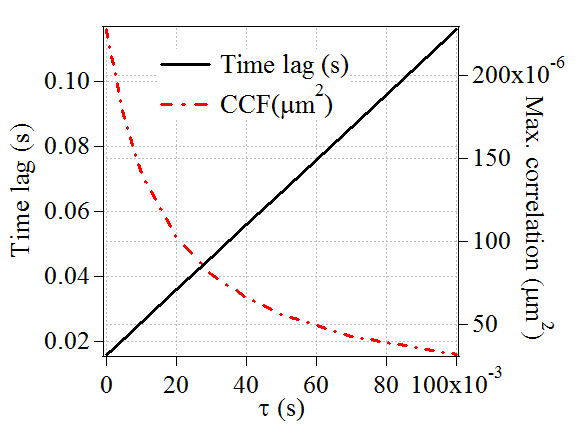
Figure 3: The plot of the maximum correlations and the corresponding time lags with respect to the Maxwell time constant $\tau$. Other parameters are chosen as in Fig. 1.

II.3 Coupled motion in a viscous fluid:

The coupled dynamics in viscous fluid can be obtained by assuming $\tau\rightarrow 0$ in the above equations. It is clear from Equs. (35), (36) and (37) that the correlation functions in frequency domain converge to

$$C_{ii}(\omega)=2k_{B}T\frac{\bigl{[}\frac{\omega^{2}}{\zeta_{0}}+\frac{k_{j}^{2}}{\zeta_{0}^{3}}(1-\varepsilon^{2})\bigr{]}}{\bigr{[}\bigl{\{}\omega^{2}-\frac{k_{i}k_{j}}{\zeta_{0}^{2}}(1-\varepsilon^{2})\bigl{\}}^{2}+\bigl{\{}(\frac{k_{i}+k_{j}}{\zeta_{0}}\omega)^{2}\bigr{\}}\bigl{]}}$$ (42)

and

$$C_{ij}(\omega)=C_{ji}(\omega)=$$

$$2k_{B}T\frac{\varepsilon\bigl{[}\frac{k_{i}k_{j}}{\zeta_{0}^{3}}(1-\varepsilon^{2})-\frac{\omega^{2}}{\zeta_{0}})\bigr{]}}{\bigr{[}\bigl{\{}\omega^{2}-\frac{k_{i}k_{j}}{\zeta_{0}^{2}}(1-\varepsilon^{2})\bigl{\}}^{2}+\bigl{\{}(\frac{k_{i}+k_{j}}{\zeta_{0}}\omega)^{2}\bigr{\}}\bigl{]}}$$ (43)

$\varepsilon\rightarrow 0$ implies zero hydrodynamic coupling which yields

$$C_{ii}(\omega)=\frac{2k_{B}T/\zeta_{0}}{\omega^{2}+\frac{k_{i}^{2}}{\zeta_{0}^{2}}}$$ (44)

and

$$C_{ij}(\omega)=C_{ji}(\omega)=0$$ (45)

In the similar way as described in the subsection II.2, the correlation functions in a viscous fluid in the time domain are of similar form as Equs. (38), (39) and (40) where the parameters will be changed to $a_{ii}=\frac{2k_{B}T}{{}^{\zeta_{0}^{3}}}\bigl{\{}k_{j}^{2}(1-\varepsilon^{2})\bigr{\}}$, $b_{ii}=\frac{2k_{B}T}{\zeta_{0}}$, $a_{ij}=-\frac{2k_{B}T}{\zeta_{0}^{3}}\varepsilon\bigl{\{}k_{i}k_{j}(1-\varepsilon^{2})\bigr{\}}$, $b_{ij}=-\frac{2k_{B}T}{\zeta_{0}}\varepsilon$ $\omega_{0}=\frac{k_{i}k_{j}}{\zeta_{0}^{2}}(1-\varepsilon^{2})$, $c=\frac{k_{i}+k_{j}}{\zeta_{0}}$ and $\nu_{1}=\sqrt{c^{2}-4\omega_{0}}$. Where, $i,\,j=1,\,2$ and $i\neq j$. In the expression of MSD, Eq. (41), one can put $\tau\rightarrow 0$ and $k_{i}\rightarrow 0$ and can get $\left\langle\Delta x_{i}^{2}(t)\right\rangle=\frac{2k_{B}T}{\zeta_{0}}t=2Dt.$ $D$ is the diffusion constant. For uncoupled motion in viscoelastic fluid, $\varepsilon=0$ and $\tau\neq 0$ and then $\left\langle\Delta x_{i}^{2}(t)\right\rangle=\frac{2k_{B}T}{\zeta_{0}+k_{i}\tau}t=2D_{r}t$. $D_{r}=\frac{k_{B}T}{\zeta_{0}+k_{i}\tau}$ is the generalized diffusion coefficient Volkov and Leonov (1996). It has been shown in Fig. 4 as a linear fit to the MSD values corresponding to very low time-lags where the effect of the trap is negligible.

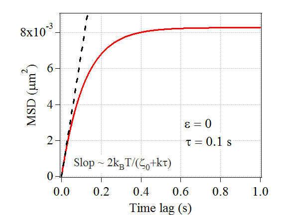
Figure 4: The uncoupled mean-square displacement (MSD) of one of the particle against time-lag for $\tau=0.1\,s$ in red line. $k=1\,\mu N/m$. The black dashed line is the straight line fit to the initial portion of the MSD curve. The slope of the straight line is $\frac{2k_{B}T}{\zeta_{0}+k_{i}\tau}$.

III Conclusions

In conclusion, a phenomenological theory of the equilibrium dynamics of two hydrodynamically coupled Brownian harmonic oscillators in a Maxwell fluid in low Reynolds numbers approximation has been presented. The response functions have been calculated and shown that these are drastically different from the reported functions in a viscous fluid. For instance, the dependency of the mutual response function on the Maxwell time constant $\tau$ which has been shown. Therefore, the formulated response functions derived in this paper can be used to perform rheological measurements in Maxwell fluid as it is done before in a viscous fluid. Further, the correlation between the noises present on the particles has been calculated and shown that such problem of the coupled Brownian motion with the simplest viscoelastic liquid can be reduced to the statistical description of an extended dynamical system subjected to a delta-correlated random force. Consequently, the generalized susceptibility of the system has been calculated and then used to calculate the position correlation functions in the frequency and the time domain. It is clear from the cross-correlation function that the two particles have time-delayed correlation and the time delay is a linear function of $\tau$ . In addition, the corresponding correlation depends on $\tau$ exponentially. Thereupon, the mean-square displacement functions of the two particles have been calculated which reveals the generalized diffusion coefficient $D_{r}=\frac{2k_{B}T}{\zeta_{0}+k_{i}\tau}$ in a Maxwell fluid in the approximation of the negligible hydrodynamic coupling, which is known to scientific community. The statistical descriptions which are derived in this paper, converge to the description in a purely viscous fluid when the Maxwell time constant $\tau$ tends to zero . Only the zero-frequency viscosity $\eta_{0}$ is incorporated in the Maxwell model as dissipation mechanism. Thus, the back ground viscosity, which is defined as the viscosity of a viscoelastic medium at $\omega\rightarrow\infty$, is neglected. Hence, in future, the reported theory can be extended using more generalized forms, like the jeffreys’ model, representing viscoelasticity which can disclose much more interesting facts.

References

• Einstein (1905) A. Einstein, Ann. Phys.(Leipzig) 17, 549 (1905).
• Von Smoluchowski (1906) M. Von Smoluchowski, Annalen der physik 326, 756 (1906).
• Volkov and Leonov (1996) V. Volkov and A. I. Leonov, The Journal of chemical physics 104, 5922 (1996).
• Grimm et al. (2011) M. Grimm, S. Jeney,  and T. Franosch, Soft Matter 7, 2076 (2011).
• Tassieri et al. (2010) M. Tassieri, G. M. Gibson, R. Evans, A. M. Yao, R. Warren, M. J. Padgett,  and J. M. Cooper, Physical Review E 81, 026308 (2010).
• Mason and Weitz (1995) T. G. Mason and D. Weitz, Physical review letters 74, 1250 (1995).
• Meiners and Quake (1999) J.-C. Meiners and S. R. Quake, Physical review letters 82, 2211 (1999).
• Martin et al. (2006) S. Martin, M. Reichert, H. Stark,  and T. Gisler, Physical review letters 97, 248301 (2006).
• Paul et al. (2017) S. Paul, A. Laskar, R. Singh, B. Roy, R. Adhikari,  and A. Banerjee, Physical Review E 96, 050102 (2017).
• Paul et al. (2018) S. Paul, R. Kumar,  and A. Banerjee, Physical Review E 97, 042606 (2018).
• Brust et al. (2013) M. Brust, C. Schaefer, R. Doerr, L. Pan, M. Garcia, P. Arratia,  and C. Wagner, Physical Review Letters 110, 078305 (2013).
• Ayala et al. (2016) Y. A. Ayala, B. Pontes, D. S. Ether, L. B. Pires, G. R. Araujo, S. Frases, L. F. Romão, M. Farina, V. Moura-Neto, N. B. Viana, et al., BMC biophysics 9, 5 (2016).
• Doi and Edwards (1988) M. Doi and S. F. Edwards, The theory of polymer dynamics, Vol. 73 (oxford university press, 1988).
• Crocker et al. (2000) J. C. Crocker, M. T. Valentine, E. R. Weeks, T. Gisler, P. D. Kaplan, A. G. Yodh,  and D. A. Weitz, Physical Review Letters 85, 888 (2000).
• Crocker and Hoffman (2007) J. C. Crocker and B. D. Hoffman, Methods in cell biology 83, 141 (2007).
• Gardiner (1984) C. W. Gardiner, Journal of the Optical Society of America B: Optical Physics, Volume 1, Issue 3, June 1984, p. 409 1, 409 (1984).
• Kubo (1966) R. Kubo, Reports on progress in physics 29, 255 (1966).