A Note on QR-Based Model Reduction: Algorithm, Software, and Gravitational Wave Applications

Abstract

While the proper orthogonal decomposition (POD) is optimal under certain norms it’s also expensive to compute. For large matrix sizes, it is well known that the QR decomposition provides a tractable alternative. Under the assumption that it is rank–revealing QR (RRQR), the approximation error incurred is similar to the POD error and, furthermore, we show the existence of an RRQR with exactly same error estimate as POD. To numerically realize an RRQR decomposition, we will discuss the (iterative) modified Gram Schmidt with pivoting (MGS) and reduced basis method by employing a greedy strategy. We show that these two, seemingly different approaches from linear algebra and approximation theory communities are in fact equivalent. Finally, we describe an MPI/OpenMP parallel code that implements one of the QR-based model reduction algorithms we analyze. This code was developed with model reduction in mind, and includes functionality for tasks that go beyond what is required for standard QR decompositions. We document the code’s scalability and show it to be capable of tackling large problems. In particular, we apply our code to a model reduction problem motivated by gravitational waves emitted from binary black hole mergers and demonstrate excellent weak scalability on the supercomputer Blue Waters up to $32,768$ cores and for complex, dense matrices as large as $10,000$-by-$3,276,800$ (about half a terabyte in size).

1 Introduction

Algorithms to compute low-rank matrix approximations have enabled many recent scientific and engineering advances. In this CiSE special issue, we summarize the theoretical properties of the most influential low-rank techniques. We also show two of the most popular techniques are algorithmically equivalent and describe a massively parallel code for QR-based model reduction that has been used for gravitational wave applications. This preprint is an expanded, more technical version of the manuscript published in IEEE’s Computing in Science & Engineering.

In this paper we consider both practical and theoretical low-rank approximations found by singular value decomposition (SVD) or QR decomposition of a matrix $S$, presenting error estimates, algorithms and properties of each. Both decompositions can be used, for example, to compute a low-rank approximation to a matrix (a common task in numerical linear algebra) or provide a high-fidelity approximation space suitable for model order reduction (a common task in engineering or approximation theory).

For certain norms an SVD-based approximation is optimal. However, for many large problems the (classical) SVD becomes problematic in terms of its memory footprint, FLOP count, and scalability on many-core machines. By comparison, QR-based model reduction is computationally competitive; it carries a lower FLOP count, is easily parallelized, and has a small inter-process communication overhead, thereby allowing one to efficiently utilize many-core machines. Indeed, for large matrices some SVD algorithms are based on QR decompositions [17]. Furthermore, for certain matrices $S$, we will show that the SVD and a special class of QR decompositions share similar approximation properties.

We are especially interested in the setting where the snapshot (or “data”) matrix may be too large to load into memory thereby precluding straightforward use of the singular value or, equivalently, a proper orthogonal decomposition (POD). In order to salvage an SVD approach, randomized or hierarchical methods can be used. QR factorizations have long been recognized as an alternative low-rank approximation. For instance the rank revealing QR (RRQR) factorization [14, 13, 15, 24] computes a decomposition of a matrix $S\in\mathbb{R}^{N\times M}$ as

$$S\Pi=QR=Q\left[\begin{array}[]{cc}R_{11}&R_{12}\\ 0&R_{22}\end{array}\right],$$ (1.1)

where $Q\in\mathbb{R}^{N\times N}$ is orthogonal, $R_{11}\in\mathbb{R}^{k\times k}$ is upper triangular, $R_{12}\in\mathbb{R}^{k\times(M-k)}$, and $R_{22}\in\mathbb{R}^{(N-k)\times(M-k)}$. The column permutation matrix $\Pi$ is usually chosen such that $\|R_{22}\|_{2}$ is small and $R_{11}$ is well-conditioned. This factorization (1.1) was introduced in [24], and the first algorithm to compute it is based on the QR factorization with column pivoting [11]. We also refer to a recent work on this subject [18].

While an RRQR always exists (see Sec. 5.1), it may be computationally challenging to find. We shall consider two specific QR strategies: modified Gram Schmidt (MGS) and a reduced basis method using a greedy strategy (RB–greedy). Although the former algorithm is widely known within the linear algebra community, the latter has become extremely popular in the approximation and numerical analysis communities [7, 19, 10]. We show that finite dimensional versions of these two approaches produce equivalent basis sets and discuss their error estimates. While for a generic $S$ these algorithms may not provide a RRQR, in all practical settings with which we are familiar these algorithms are rank revealing and the resulting RRQR approximation error is of the same order as the SVD/POD. There may be additional advantages when the columns form the basis as opposed to linear combinations over all columns; a typical example is column subset selection [40].

As a rank-revealer, the column pivoted QR decomposition is known to fail on, for example, Kahan’s matrix [29]. A formal fix to this is discussed in [18, Section 4], see also [20] where several related issues were analyzed and the appropriate algorithmic fixes were discussed. Nevertheless, matricies like the Kahan one are rarely (if ever) encountered in model reduction problems. In typical cases, the approximation properties of QR-based model reduction is summarized as follows. The RB-greedy error in Algorithm 3 is given by $\max_{1\leq i\leq M}\|s_{i}-Q_{k}Q_{k}^{T}s_{i}\|_{2}$ where $s_{i}\in\mathbb{R}^{N}$ are columns of $S$ and $Q_{k}\in\mathbb{R}^{N\times k}$ (see Definition 3). The state-of-the-art results presented in [19, 7] provide us an a priori behavior of this error: if the Kolmogorov $n$-width (best approximation error) decays exponentially with respect to $k$ so does the greedy error. For many model reduction problems, smoothness with respect to parametric variation plays an essential role. For smooth models the $n$-width (and thus the greedy error) is expected to decay exponentially fast [19, 34].

We will show that MGS is equivalent to RB–greedy (see Proposition 14) and derive error estimates for both algorithms. We recall error estimates for the full QR decomposition in Theorems 8–10 and, under the assumption that this decomposition is an RRQR, we show that the underlying error is of same order as POD in the $\ell^{2}$–norm. Existence of an optimal RRQR decomposition is shown. We give a reconstruction strategy in Section 5.2.2, which is cheaper than, but as accurate as, the POD.

A key contribution of this paper is the development of a publicly available code  that implements the RB-greedy algorithm parallelized with message passing interface (MPI) and OpenMP. Unlike other parallelized QR codes, our software is designed with model reduction in mind and uses a simple interface for easy integration with model-generation codes. Sec. 6 documents the code’s performance for dense matrices with sizes as large as $10^{7}$-by-$10^{4}$. Model reduction is sometimes combined with an empirical interpolation method, and we briefly document our codes efficiency in computing empirical interpolants [32, 16] using many thousands of basis. We focus on generating empirical interpolants for the acceleration of gravitational wave parameter inference [6, 2, 37, 12, 33]; the QR-accelerated inference codes have been used in the most recent set of gravitational wave detections [2, 4, 3]. For such large dimensional reduction problems, an efficient, parallelized code [1] running on thousands of cores has proven essential.

The outline of this paper is as follows. In Section 2 we introduce projection based reduced order model (ROM) techniques. We summarize well known facts about POD/SVD-based model reduction in Section 3 such as optimality results and error bounds. Section 4 discusses the full QR factorization and the resulting approximation. Section 5 motivates rank revealing QR-based model reduction as a computationally efficient alternative and provides error bounds and comparisons to POD. Two specific QR-based algorithms (MGS and RB–greedy) are considered and compared in Section 5.2.1, and reconstruction technique is presented in Section 5.2.2. Section 6 documents performance and scalability tests of the open-source greedycpp code developed in this paper [1].

2 Dimensional reduction techniques

Let us assume we are given $M$ samples $s_{1},...,s_{M}\in\mathbb{R}^{N}$ and an associated snapshot matrix $S=(s_{1},...,s_{M})\in\mathbb{R}^{N\times M}$ whose $i^{\mathrm{th}}$ column is $s_{i}$. Each $s_{i}$ corresponds to a realization of an underlying parameterized model: we evaluate the model at selected parameter values and designate the solution as $s_{i}$.

Within the setting just described, reduced order models are derived from a low-rank approximation for $S$. As briefly summarized in this section, the SVD and QR exposes certain kinds of low-rank approximations. We introduce a few definitions.

Definition 1 (full SVD).

Given a matrix $S\in\mathbb{R}^{N\times M}$, the full SVD of $S$ is

$$S=V\Sigma W^{T},$$

where $V\in\mathbb{R}^{N\times N},\Sigma\in\mathbb{R}^{N\times M},W\in\mathbb{R}^{M\times M}$. In addition, $V$ and $W$ are orthogonal matrices, and $\Sigma$ is a diagonal matrix with non-increasing entries, known as singular values. The $k^{\tt th}$ singular value is denoted by $\sigma_{k}$.

From the singular values we define the ordinary and numerical-ranks of a matrix as follows:

Definition 2 (ordinary- and numerical-ranks of $S$).

Let $S\in\mathbb{R}^{N\times M}$ be a matrix whose singular values $\{\sigma_{i}\}_{i=1}^{M}$ are arranged in a decreasing order. Then $S$ is said to have numerical rank $k$ if

$$\sigma_{k+1}\approx\epsilon_{\tt mach}$$

where $\epsilon_{\tt mach}$ is the machine precision and a standard, or ordinary-rank, if

$$\sigma_{k+1}=0\,.$$

Definition 3 (full QR).

The full $QR$ factorization of $S\in\mathbb{R}^{N\times M}$ is

$$S\Pi=QR=\left[\begin{array}[]{cc}Q_{k}&Q_{N-k}\end{array}\right]\left[\begin{array}[]{cc}R_{11}&R_{12}\\ 0&R_{22}\end{array}\right].$$ (2.4)

where $Q_{k}\in\mathbb{R}^{N\times k}$ and $Q_{N-k}\in\mathbb{R}^{N\times(N-k)}$ are orthogonal, $R_{11}\in\mathbb{R}^{k\times k}$ is upper triangular, $R_{12}\in\mathbb{R}^{k\times(M-k)}$, and $R_{22}\in\mathbb{R}^{(N-k)\times(M-k)}$.

The role of a permutation matrix $\Pi\in\mathbb{R}^{M\times M}$ in (2.4) is to swap columns of $S$ and is crucial for achieving QR-based model reduction. Different QR algorithms prescribe different rules for discovering $\Pi$. If QR is not pivoted, then we define the permutation matrix as identity.

Of particular interest is the RRQR decomposition. There are several different ways of defining an RRQR, one of them [29, 15] says that the factorization (2.4) is an RRQR if:

Definition 4 (RRQR).

Assume $S\in\mathbb{R}^{N\times M}$ has numerical rank $k$, if

$$\sigma_{\tt min}(R_{11})\gg\|R_{22}\|_{2}\approx\epsilon_{\tt mach}$$

then the factorization $S\Pi=QR$ is called a Rank Revealing QR factorization (RRQR) of $S$.

From [29, Lemma 1.2] we recall that the following holds for any $\Pi$

$$\sigma_{k}(S)\geq\sigma_{\rm min}(R_{11})\quad\mbox{and}\quad\|R_{22}\|_{2}=\sigma_{\rm max}(R_{22})\geq\sigma_{k+1}(S),$$

whence Definition 4 implies

$$\sigma_{k+1}(S)\leq\|R_{22}\|_{2}=\sigma_{\rm max}(R_{22})\ll\sigma_{\rm min}(R_{11})\leq\sigma_{k}(S),$$

i.e., Definition 4 introduces a large gap between $\sigma_{k+1}(S)$ and $\sigma_{k}(S)$. Finally, we define an optimal RRQR of $S$ as follows:

Definition 5 (optimal RRQR).

$QR=S\Pi$ is an optimal RRQR of $S\in\mathbb{R}^{N\times M}$ if

$$\|S-Q_{k}Q_{k}^{T}S\|_{2}=\sigma_{k+1}.$$ (2.5)

Projection-based model reduction represents a single column of the matrix, $s_{i}$, via orthogonal projection of $s_{i}$ onto the span of the basis. Approximation errors using an SVD basis, $s_{i}-V_{k}V_{k}^{T}s_{i}$, or using a QR basis, $s_{i}-Q_{k}Q_{k}^{T}s_{i}$, are considered in the next sections. Throughout this paper we will use $V_{k}$ to denote a matrix formed by the first $k$ columns of $V$.

3 Full POD/SVD with error estimates

We first recall the POD problem formulation: A POD computes $k$ orthonormal vectors $v_{1},...,v_{k}\in\mathbb{R}^{N}$ which provide an optimal solution to

$$\epsilon_{*}:=\min_{Y_{k}\in\mathbb{R}^{N\times k}}\|S-Y_{k}Y_{k}^{T}S\|_{*}^{2}$$ (3.1)

where $*$ is either the Frobenius $(F)$ or matrix 2-norm. It is well known that the $*$–norm solution to (3.1) can be computed by first performing a SVD of $S=V\Sigma W^{T}$, from which $Y_{k}=V_{k}=(v_{1},...,v_{k})\in\mathbb{R}^{N\times k}$ is simply the first $k$ columns of $V$.

We shall assume, for definiteness, a full SVD of $S$. We will frequently require matrices with zeros in all columns after $k+1$ and shall denote these with a superscript “$0$”. For example, $V_{k}V_{k}^{T}V:=V_{k}^{0}$ is $V$ with zeros in columns $k+1$ to $N$. Using this notation it is easy to see that the POD approximation of $S$

$$V_{k}V_{k}^{T}S=V_{k}V_{k}^{T}V\Sigma W^{T}=V_{k}^{0}\Sigma W^{T}=V\Sigma_{k}^{0}W^{T}=\sum_{i=1}^{k}\sigma_{i}v_{i}w_{i}^{T}$$ (3.2)

is exactly a sum of $k$ rank-one matrices, where $\Sigma_{k}^{0}$ is $\Sigma$ with zeros in columns $k+1$ to $N$. This illustrates the close connection of POD with the partial SVD factorization $V\Sigma_{k}^{0}W^{T}$.

3.1 2-norm and $F$-norm POD error estimates

We briefly recall standard POD error estimates.

Lemma 6.

Let $A$ and $B$ be two matrices. If $A$ is orthogonal then $\|AB\|_{*}=\|B\|_{*}$; if $B$ is orthogonal, then $\|AB\|_{*}=\|A\|_{*}$.

Theorem 7 (POD error estimates).

Given $S\in\mathbb{R}^{N\times M}$ with SVD of $S=V\Sigma W^{T}$, then

1. $\|S-V_{k}V_{k}^{T}S\|_{F}^{2}=\sum_{j=k+1}^{\min{\{M,N\}}}\sigma_{j}^{2}$.

2. $\|S-V_{k}V_{k}^{T}S\|_{2}=\sigma_{k+1}$.

Proof.

The proof is standard but we recall it here for completeness. By Lemma 6 and Equation (3.2)

$$\|S-V_{k}V_{k}^{T}S\|_{*}^{2} =\|V\Sigma-V_{k}V_{k}^{T}V\Sigma\|_{*}^{2}=\|\Sigma-\Sigma_{k}^{0}\|_{*}^{2}\,.$$

From the definition of $F$ and 2 norms, we deduce

$$\|\Sigma-\Sigma_{k}^{0}\|_{F}^{2}=\sum_{j=k+1}^{\min{\{m,N\}}}\sigma_{j}^{2},\qquad\|\Sigma-\Sigma_{k}^{0}\|_{2}=\sigma_{k+1}\,,$$

which completes the proof. ∎

From Theorem 7, errors measured in the $F$-norm require computation of all singular values, which can be expensive. Using the 2-norm requires only the first $k+1$ singular values, which motivates a choice of $\sigma_{k+1}<\tau$ to control the approximation error $\tau$ in Algo. 1. In practice, we always choose $\tau$ larger than machine precision.

Algorithm 1 POD

1:Input: Snapshot matrix $S=(s_{1},...,s_{M})\in\mathbb{R}^{N\times M}$ and tolerance $\tau>0$

2:Output: $V_{k}=(v_{1},...,v_{k})\in\mathbb{R}^{N\times k}$

3:Compute the singular value decomposition $S=V\Sigma W^{T}$.

4:Find smallest index $k$ such that the singular values satisfy $\sigma_{k+1}<\tau.$

5:Return the first $k$ columns $V_{k}=(v_{1},...,v_{k})\in\mathbb{R}^{N\times k}$ of $V$.

4 Full QR with error estimates

In Theorem 7 we showed that POD provides the best rank $k$ $*$-norm approximation to the snapshot matrix $S$. In Theorem 8 we will see that under the assumption that the decomposition is an RRQR (according to Def.  4) the resulting approximation error using full QR factorization is of the same order as POD-based approximation error. In Section 4.1 we will first discuss the $*$–norm error estimates and we conclude with max-norm error estimates in Section 4.2. Note that a QR decomposition always exists but need not be unique [39].

4.1 2-norm and $F$-norm error estimates

We define the QR-based error for the decomposition (2.4) as

$$\epsilon_{*}^{QR}(\Pi):=\|S\Pi-Q_{k}Q_{k}^{T}S\Pi\|_{*}=\|S-Q_{k}Q_{k}^{T}S\|_{*},$$ (4.1)

where $*$ could be either 2-norm or $F$-norm. The QR-based approximation error depends on the permutation matrix implicitly through $Q_{k}$. To avoid extra notation, we sometimes omit writing $S\Pi$ and assume $S$ is already pivoted when it is clear from context.

Let

$$R=\overline{V}\Sigma\overline{W}^{T},$$ (4.2)

be the SVD of $R$ where we have added over-bars to make a clear distinction with the SVD of $S$ and, recall, that $S$ and $R$ have the same singular value spectrum (hence $\overline{\Sigma}=\Sigma$). Furthermore $\overline{V}\in\mathbb{R}^{N\times N}$, $\overline{W}\in\mathbb{R}^{M\times M}$ and $\Sigma\in\mathbb{R}^{N\times M}$. Let

$$Q_{k}^{0}:=Q_{k}Q_{k}^{T}Q\,$$ (4.3)

be $Q$ with zeros in columns from $k+1$ to $N$, $\overline{V}_{k,0}$ is $\overline{V}$ with zeros from rows $k+1$ to $N$, and $\overline{V}_{N-k,0}$ is $\overline{V}$ with zeros from rows $1$ to $k$. Observe that

$$Q_{k}^{0}\overline{V}=Q\overline{V}_{k,0}.$$ (4.4)

Theorem 8 (full QR $*$-norm error estimate).

Let $Q_{k}\in\mathbb{R}^{N\times k}$ denote the first $k$ columns of $Q$, then

$$\epsilon_{*}^{QR}(\Pi)=\|S-Q_{k}Q_{k}^{T}S\|_{*}=\|\overline{V}_{N-k,0}\Sigma\|_{*}=\|R_{22}\|_{*},$$ (4.5)

where $*$ is either 2-norm or F-norm. A proof can be found in Ref. [13]

Proof.

To show the first equality, we use Lemma 6,  (4.2), and  (4.3), we deduce

$$\|S-Q_{k}Q_{k}^{T}S\|_{*} =\|QR-Q_{k}Q_{k}^{T}QR\|_{*}=\|QR-Q_{k}^{0}R\|_{*}$$

$$=\|Q\overline{V}\Sigma\overline{W}^{T}-Q_{k}^{0}\overline{V}\Sigma\overline{W}^{T}\|_{*}=\|Q\overline{V}\Sigma-Q_{k}^{0}\overline{V}\Sigma\|_{*}.$$

Invoking  (4.4), we obtain

$$\|S-Q_{k}Q_{k}^{T}S\|_{*} =\|Q\overline{V}\Sigma-Q\overline{V}_{k,0}\Sigma\|_{*}=\|(\overline{V}-\overline{V}_{k,0})\Sigma\|_{*}=\|\overline{V}_{N-k,0}\Sigma\|_{*}\,,$$

which proves the first equality in (4.5).

The proof of the second equality is similar to the proof of Theorem 7, we readily obtain

$$\|S-Q_{k}Q_{k}^{T}S\|_{*}=\|QR-Q_{k}^{0}R\|_{*}=\|R_{22}\|_{*},$$

the last equality naturally comes out as $R$ upper triangular. Thus, we conclude. ∎

Remark 9.

Invoking the optimality of POD, we notice that $\|S-V_{k}V_{k}^{T}S\|_{*}\leq\|S-Q_{k}Q_{k}^{T}S\|_{*}$. Assuming that QR is RRQR (according to Def. 4) and employing Theorem 8 we notice that the approximation error of the full QR and POD are of the same order.

4.2 Max–norm error estimate

We define the QR–based approximation error in the max-norm as

$$\epsilon_{\max}^{QR}(\Pi):=\max_{1\leq i\leq M}\|s_{i}-Q_{k}Q_{k}^{T}s_{i}\|_{2}\,,$$ (4.6)

where, for vectors, $\|\cdot\|_{2}$ is the usual Euclidean norm. Measured in the max-norm, the QR-based approximation error is given by the following result.

Theorem 10 (full QR max-norm error estimate).

Let $r_{i}$ be the $i$-th column of $R$ and $\widetilde{r}_{i}$ be a subvector of $r_{i}$ from row $k+1$ to $N$. Then the approximation error for any given $s_{i}$ is

$$\|s_{i}-Q_{k}Q_{k}^{T}s_{i}\|_{2}=\|\widetilde{r}_{i}\|_{2},\ i=1,\dots,M,$$

whence $\epsilon_{max}^{QR}=\max_{1\leq i\leq M}\|\widetilde{r}_{i}\|_{2}$.

Proof.

Invoking Lemma 6 and Equation (4.3), we deduce

$$\|s_{i}-Q_{k}Q_{k}^{T}s_{i}\|_{2}=\|Qr_{i}-Q_{k}Q_{k}^{T}Qr_{i}\|_{2}=\|Qr_{i}-Q_{k}^{0}r_{i}\|_{2}=\|\widetilde{r}_{i}\|_{2}\,,$$

thus we conclude. ∎

Corollary 11.

The following relation between the $*$ and max norm estimates for QR holds

$$\epsilon_{max}^{QR}\leq\epsilon_{*}^{QR}.$$

Proof.

Invoking Theorem 8 and Theorem 10 and the fact that $\widetilde{r}_{i}$ is the submatrix of $R_{22}$, we conclude

$$\max_{1\leq i\leq M}\|\widetilde{r}_{i}\|_{*}\leq\|R_{22}\|_{*},$$

which is due to the fact that the norm of a submatrix is less than the norm of matrix it embedded in. ∎

5 Specific QR algorithms

The goal of this section is to discuss different QR decomposition strategies (that is to say, the pivoting strategy) useful for low-rank approximation. We first consider the optimal RRQR whose 2-norm error estimates exactly match the POD error estimates (see Theorem 7). Next we consider practical RRQR algorithms which are implementable. For the practical RRQR, in Section 5.2, we will discuss two algorithms: modified Gram–Schmidt (MGS) with pivoting and a reduced basis method using a greedy approach (RB–greedy). We show that these methods are in fact equivalent in certain settings. We will derive the error estimates and furnish FLOP counts. In Section 5.2.2 we discuss a QR-reconstruction strategy with error estimates similar to POD.

5.1 Optimal RRQR

In this section we show that an optimal QR-based approximation exits (although its not necessarily unique). We will provide a constructive proof. We begin by computing the SVD of $S$ as

$$S=V\Sigma W^{T}=\left[\begin{array}[]{cc}V_{k}&V_{N-k}\end{array}\right]\left[\begin{array}[]{cc}\Sigma_{k}&0\\ 0&\Sigma_{N-k,M-k}\end{array}\right]\left[\begin{array}[]{cc}W_{k}^{T}\\ W_{M-k}^{T}\end{array}\right]$$ (5.5)

$$=V_{k}\Sigma_{k}W_{k}^{T}+V_{N-k}\Sigma_{N-k,M-k}W_{M-k}^{T}.$$ (5.6)

In addition, let

$$\mathcal{QR}=\Sigma_{k}W_{k}^{T},$$ (5.7)

be a QR factorization of $\Sigma_{k}W_{k}^{T}$. Finally, we set

$$Q_{k}=V_{k}\mathcal{Q}\,.$$ (5.8)

We will prove that such a $Q_{k}$ will lead to the optimal RRQR according to Def. 4.

Theorem 12 (existence of optimal RRQR and equivalence to POD error).

Let $S\in\mathbb{R}^{N\times M}$, then an optimal RRQR (according to Def. 4) of $S$ exists, with

$$Q=\left[\begin{array}[]{cc}Q_{k}&Q_{N-k}\end{array}\right]\quad\mbox{and}\quad R=\left[\begin{array}[]{cc}\mathcal{R}\\ 0\end{array}\right],$$ (5.9)

where $\mathcal{R}$ and $Q_{k}$ are defined in (5.7) and (5.8) respectively and $Q_{N-k}\in\mathbb{R}^{N\times(N-k)}$ is defined such that $Q^{T}Q=I$. The following estimate holds

$$\|S-Q_{k}Q_{k}^{T}S\|_{2}=\|S-V_{k}V_{k}^{T}S\|_{2}=\sigma_{k+1}.$$ (5.10)

where $V_{k}$ is as defined in Theorem 7.

Proof.

The proof is constructive. Using the SVD of $S$ from (5.5), it is not difficult to see that

$$\|S-V_{k}\Sigma_{k}W_{k}^{T}\|_{2}=\sigma_{k+1}.$$ (5.11)

Next we use (5.8), (5.5), and invoke the orthogonality of $V$ to yield

$$\|S-Q_{k}Q_{k}^{T}S\|_{2} =\|S-V_{k}\mathcal{Q}\mathcal{Q}^{T}V_{k}^{T}S\|_{2}$$

$$=\|S-V_{k}\mathcal{Q}\mathcal{Q}^{T}V_{k}^{T}\left(V_{k}\Sigma_{k}W_{k}^{T}+V_{N-k}\Sigma_{N-k,M-k}W_{M-k}^{T}\right)\|_{2}$$

$$=\|S-V_{k}\mathcal{Q}\mathcal{Q}^{T}\Sigma_{k}W_{k}^{T}\|_{2}\,.$$

Notice that $\mathcal{Q}\mathcal{Q}^{T}\Sigma_{k}W_{k}^{T}=\mathcal{Q}\mathcal{Q}^{T}\mathcal{QR}=\mathcal{QR}=\Sigma_{k}W_{k}^{T}$, where we have used (5.5), we arrive at

$$\|S-Q_{k}Q_{k}^{T}S\|_{2}=\|S-V_{k}\Sigma_{k}W_{k}^{T}\|_{2}=\sigma_{k+1},$$

therefore (5.11) in conjunction with Theorem 7 enables us to obtain the asserted equality (5.10). ∎

We do not offer an efficient algorithm to calculate the optimal RRQR other than to first calculate a potentially expensive SVD as in proof. Notice that in this case the optimal RRQR’s permutation matrix $\Pi$ is the identity. In particular, the QR factorization constructed in the proof does not arise from the QR pivoting strategies of Sec. 5.2, and to the best of our knowledge the matrix $Q_{k}$ cannot in general be constructed as a column subset of $S$.

The estimate in (5.10) states that 2-norm error in POD (Theorem 7) is same as the optimal RRQR. We reemphasize that, although the proof above is constructive, it does not provide a numerical recipe to compute QR factorization. This is the subject of next section.

Corollary 13 (optimal RRQR and ordinary $k$–rank matrix).

If $S\in\mathbb{R}^{N\times M}$ has an ordinary rank $k$ then under the assumptions of Theorem 12, $S=QR$ with $Q$ and $R$ defined in (5.9).

Proof.

Using (5.7) and (5.8) we first notice that

$$V_{k}\Sigma_{k}W_{k}^{T}=V_{k}\mathcal{QR}=Q_{k}R=QR.$$

Since $S$ has ordinary rank $k$ therefore $\sigma_{k+1}=0$, invoking (5.11) we obtain the assertion. ∎

5.2 Practical RRQR

This section is devoted to two algorithms that aim to compute an RRQR. Algorithm 2 is the modified Gram-Schmidt (MGS) with pivoting [25]. Algorithm 3 is a particular flavor of the (by now) standard reduced basis (RB)-greedy algorithm [7, 19, 10]. RB-greedy is a popular tool employed in the construction of model reduction schemes for parameterized partial differential equations. We present each algorithm in their standard presentation, and in Proposition 14 show these algorithms to be equivalent when the snapshots $s_{i}$ are elements of an $N$–dimensional Euclidean vector space. Theorem 10 and Corollary 17 motivate the choice of stopping criteria, which relies on diagonal entries of $R$ being non-increasing. This aspect is discussed in Corollary 17.

5.2.1 Equivalence of the MGS and RB-greedy algorithms

The MGS with pivoting and RB-greedy algorithms are as follows:

Algorithm 2 MGS with pivoting

1:Input: $S=(s_{1},...,s_{M})$, $\tau>0$

2:Output: $Q_{k}=(q_{1},...,q_{k})$

3:Set $V=S$ and $k=1$

4:Set $R(1,1)=\mbox{max}_{j}\|V(:,j)\|_{2}$

5:while $R(k,k)>\tau$ do

6:    $i$ = $\mbox{arg max}_{j}\|V(:,j)\|_{2}$

7:    $\Pi(k,i)=1$

8:    $R(k,k)=\|V(:,i)\|_{2}$

9:    $Q(:,i)=V(:,i)/R(k,k)$

10:    for $j=k+1$ to $M$ do

11:       $R(k,j)=Q(:,k)^{T}V(:,j)$

12:       $V(:,j)=V(:,j)-R(k,j)Q(:,k)$

13:    end for

14:    $k=k+1$

15:end while

Algorithm 3 RB-greedy

1:Input: $S=(s_{1},...,s_{M})$, $\tau>0$

2:Output: $Q_{k}=(q_{1},...,q_{k})$

3:Set $k=0$

4:Define $\hat{\sigma}_{0}(s_{i})=\|s_{i}\|_{2}$

5:$j(0)=\mbox{arg sup}_{i}\hat{\sigma}_{0}(s_{i})$

6:Define $\hat{\sigma}_{0}=\hat{\sigma}_{0}(s_{j(0)})$

7:$q_{1}=s_{j(0)}/\|s_{j(0)}\|_{2}$

8:while $\hat{\sigma}_{k}\geq\tau$ do

9:    $k=k+1$

10:    $\hat{\sigma}_{k}(s_{i})=\|s_{i}-Q_{k}Q_{k}^{T}s_{i}\|_{2}$ $\forall s_{i}\in S$

11:    $j(k)=\mbox{arg sup}_{i}\hat{\sigma}_{k}(s_{i})$

12:    $\hat{\sigma}_{k}=\hat{\sigma}_{k}(s_{j(k)})$

13:    $q_{k+1}=s_{j(k)}-Q_{k}Q_{k}^{T}s_{j(k)}$

14:    $q_{k+1}:=q_{k+1}/\|q_{k+1}\|_{2}$

15:end while

Proposition 14.

For a matrix $S\in\mathbb{R}^{N\times M}$, the RB-greedy Algo. 3 is equivalent to the MGS with column pivoting Algo. 2. Moreover, the diagonal entries of $R$ are non–increasing, i.e.,

$$R(1,1)\geq R(2,2)\geq\dots\geq R(M,M)\geq 0,$$ (5.12)

Proof.

It is sufficient to show their pivoting strategies are equivalent. In Algo. 3, the $k$th column pivot is

$$j(k)=\mbox{arg max}_{i}\|s_{i}-\sum_{j=1}^{k-1}q_{j}^{T}s_{i}q_{j}\|_{2}\,.$$

For MGS with column pivoting Algo. 2 we have

$$\mbox{arg max}_{i}\|v^{(k)}_{i}\|_{2}\,,$$

where $v^{(k)}_{i}$ is defined from a recurrence relation

$$v^{(k)}_{i}\leftarrow\zeta:=v^{(k)}_{i}-q_{k}^{T}v^{(k)}_{i}q_{k}\,,\qquad v^{(1)}_{i}=s_{i}\,.$$

Thus using the orthogonality of $q_{k}$ we obtain

$$\zeta=v_{i}^{(1)}-\sum_{j=1}^{k-1}q_{j}^{T}v_{i}^{(1)}q_{j}=s_{i}-\sum_{j=1}^{k-1}q_{j}^{T}s_{i}q_{j}$$

Hence, the selection of pivots

$$\mbox{arg max}_{i}\|s_{i}-\sum_{j=1}^{k-1}q_{j}^{T}s_{i}q_{j}\|_{2}=\mbox{arg max}_{i}\|v^{(k)}_{i}\|_{2}\,,$$

are equivalent. ∎

Remark 15.

As presented, the MGS with pivoting carries a greater memory overhead. In terms of operation counts the MGS steps 6 and 12 are dominant, requiring $2N(M-j+1)$ and $4N(M-j)$ FLOPs at iteration $j$. Then the total count is

$$\sum_{j=1}^{k}(4N)(M-j)+2N(M-j-1) \approx\sum_{i=1}^{k}6NM-\sum_{j=1}^{k}(6Nj)=6kNM-3Nk^{2}\,,$$ (5.13)

after $k$ steps. The RB-greedy’s dominant cost is the pivoting step 10, where, after $k$ iterations, the accumulated FLOP count is

$$\sum_{i=1}^{k}(3N(i-1)+N+2N)M=\sum_{i=1}^{k}3NMi\approx\frac{3}{2}k^{2}NM\,.$$ (5.14)

Remark 16.

These algorithms may be modified to improve memory overhead, FLOP counts, or conditioning. For very large problems the dominant FLOP count of Algo. 3 can be dramatically reduced if one stores the projections $Q_{k}Q_{k}^{T}s_{i}$ from each previous step; this would essentially amount to storing a matrix $V$ as is done in the MGS with pivoting. Furthermore, the naive implementation of the classical Gram-Schmidt procedure can lead to a numerically ill-conditioned algorithm. To overcome this one should use well-conditioned orthogonalization algorithms such as the iterated Gram-Schmidt [23, 28, 36] or Householder reductions. Our implementation of Alg. 3 uses Hoffmann’s iterated Gram-Schmidt [28] which maintains orthogonality for extremely large basis sets [21]. We are unaware of results which characterize the preservation of the subspace spanned by the original vectors, but for many approximation-driven applications this is not strictly necessary.

The proof shows their pivoting strategies are equivalent. Having demonstrated the (finite dimensional) equivalence of Algorithms 2 and 3, we now discuss their properties. Recall that diagonal components of $R$ are non-increasing. The following result, which motivated the stopping criterion in Algo. 2, shows how the diagonal entires of $R$ are closely connected with the max-norm approximation error used in Algorithm 3 (see also Theorem 10).

Corollary 17.

The stopping criterion used in Algorithms 2 and 3 fulfills

$$\max_{1\leq i\leq M}\|s_{i}-Q_{k}Q_{k}^{T}s_{i}\|_{2}=R(k+1,k+1)\,.$$

Proof.

Theorem 10 exactly characterizes the error $\|\widetilde{r}_{i}\|_{2}$. Then using the definition of $R(k+1,j)$, $j=1,\dots,M$ it is not difficult to see that

$$\|\widetilde{r}_{i}\|_{2}\leq R(k+1,k+1),\ 1\leq i\leq M.$$

In addition, we pick $R(k+1,k+1)$ such that

$$R(k+1,k+1)=\max_{1\leq i\leq M}\|S(:,i)-\sum_{j=1}^{k}Q(:,j)^{T}S(:,i)Q(:,j)\|_{2}\,,$$

and since the diagonal entries of $R$ are nonincreasing, we obtain

$$R(k+1,k+1)\leq R(k,k)=\max_{1\leq i\leq M}\|S(:,i)-\sum_{j=1}^{k-1}Q(:,j)^{T}S(:,i)Q(:,j)\|_{2}$$

Then the estimate follows after using Theorem 10. ∎

We next derive a representation of the estimate in Corollary 17 in terms of the singular values of $S$.

Corollary 18.

Let $S\in\mathbb{R}^{N\times M}$ then

$$\max_{1\leq i\leq M}\|s_{i}-Q_{k}Q_{k}^{T}s_{i}\|_{2}=\Big{(}\prod_{i=1}^{k+1}\sigma_{i}\Big{)}/\Big{(}\prod_{i=1}^{k}R(i,i)\Big{)}.$$

Proof.

Denote by $S_{k+1}$ the first $k+1$ columns of $S\Pi$. Taking QR decomposition of $S_{k+1}$, we obtain

$$S_{k+1}=QR,\quad Q\in\mathbb{R}^{N\times(k+1)},\ R\in\mathbb{R}^{(k+1)\times(k+1)},$$

yielding $\det(S_{k+1})=\det(R)$. Since $\det(S_{k+1})=\prod_{i=1}^{k+1}\sigma_{i}$ and $\det(R)=\prod_{i=1}^{k+1}R(i,i)$, using Corollary 17 we arrive at the assertion. ∎

5.2.2 A reconstruction approach to QR

We recall that the POD algorithm (1) generates the optimal 2-norm basis (see Theorem 7). The goal of this section is to augment the QR with a reconstruction technique such that resulting approximation of $S$ is as accurate as POD, however the algorithm is cheaper than performing an SVD. We note that our method shares some similarities with those algorithms that perform QR decompositions as a precursor to finding the SVD (e.g. [17, 39]).

Theorem 19.

Given $S\in\mathbb{R}^{N\times M}$ with ordinary rank $k$, if $X=Q\overline{V}$, then $X_{k}=Q_{k}\mathcal{V}$, and

$$\|S-X_{j}X_{j}^{T}S\|_{2}=\sigma_{j+1}=\|S-Q_{j}Q_{j}^{T}S\|_{2}=\|S-V_{j}V_{j}^{T}S\|_{2},\quad 1\leq j\leq k.$$

Proof.

Since $S$ has ordinary rank $k$, using Corollary 13

$$R=\left[\begin{array}[]{cc}R_{11}&R_{12}\\ 0&0\end{array}\right]=\overline{V}\Sigma\overline{W}^{T}.$$

Let $R=\overline{V}\Sigma\overline{W}^{T}$ be the SVD of $R$ and

$$\mathcal{V}\Sigma_{k,M}\mathcal{W}^{T}=\left[\begin{array}[]{cc}R_{11}&R_{12}\end{array}\right],$$

be full SVD of $\left[\begin{array}[]{cc}R_{11}&R_{12}\end{array}\right]$, where $\mathcal{V}\in\mathbb{R}^{k\times k},\ \Sigma_{k,M}\in\mathbb{R}^{k\times M}$, and $\mathcal{W}\in\mathbb{R}^{M\times M}$. Then

$$R=\left[\begin{array}[]{cc}R_{11}&R_{12}\\ 0&0\end{array}\right]=\overline{V}\Sigma\overline{W}^{T}=\left[\begin{array}[]{cc}\mathcal{V}&0\\ 0&\widetilde{\mathcal{V}}\end{array}\right]\left[\begin{array}[]{cc}\Sigma_{k,M}\\ 0\end{array}\right]\mathcal{W}^{T},$$

where $\widetilde{\mathcal{V}}\in\mathbb{R}^{(N-k)\times(M-k)}$ is an arbitrary orthogonal matrix. Defining

$$X=Q\overline{V}=\left[\begin{array}[]{cc}Q_{k}&Q_{N-k}\end{array}\right]\left[\begin{array}[]{cc}\mathcal{V}&0\\ 0&\widetilde{\mathcal{V}}\end{array}\right]=\left[\begin{array}[]{cc}Q_{k}\mathcal{V}&Q_{N-k}\widetilde{\mathcal{V}}\end{array}\right]$$

leads to

$$X_{j}=Q_{k}\mathcal{V}_{j},\quad\mbox{for }1\leq j\leq k.$$

We now show that $\|S-X_{j}X_{j}^{T}S\|_{2}=\sigma_{j+1}$ for $1\leq j\leq k$, the other estimate is due to Theorem 12. Recalling $S=QR$ and $R=\overline{V}\Sigma\overline{W}^{T}$, we deduce

$$\|S-X_{j}X_{j}^{T}S\|_{2} =\|X\Sigma\overline{W}^{T}-X_{j}X_{j}^{T}X\Sigma\overline{W}^{T}\|_{2}=\|X\Sigma-X_{j}^{0}\Sigma\|_{2}$$

$$=\|X\Sigma-X\Sigma_{j}\|_{2}=\|\Sigma-\Sigma_{j}^{0}\|_{2}=\sigma_{j+1}=\|S-V_{j}V_{j}^{T}S\|_{2},$$

where $X_{j}^{0}$ is $X$ with zeros in columns $j+1$ to $N$ and the last equality is due to Theorem 7(ii). ∎

With this motivation, we introduce the following algorithm for a matrix $S\in\mathbb{R}^{N\times M}$ of numerical rank $k$.

Algorithm 4 Reconstruction Algorithm

1:Input: Samples $S=(s_{1},...,s_{M})\in\mathbb{R}^{N\times M}$, tolerance $\tau_{1},\tau_{2}>0$

2:Output: $X_{k}=(x_{1},...,x_{k})\in\mathbb{R}^{N\times k}$

3:Perform a partial $j$-term MGS with pivoting of $S$ stopping whenever $|R(j,j)|<\tau_{1}$

4:Let $S=Q_{j}R(1:j,1:M)$ be the result of step 3

5:Perform an SVD $\mathcal{V}\Sigma\mathcal{W}^{T}=R(1:j,1:M)$

6:Find $k\in\{1,\dots,j\}$ such that $\sigma_{k+1}<\tau_{2}<\sigma_{k}$

7:Return $X_{k}=Q_{k}\mathcal{V}(1:k,1:k)$

Remark 20.

Computational cost of step 3 is $\mathcal{O}(Mj^{2}+Nj^{2})$, which is less than the MGS with pivoting cost $\mathcal{O}(jNM)$ given that $j\ll N$. Steps 4-5 enrich the basis: generally speaking, the diagonal entry of $R$ decrease slower than the singular values, and so we employ the SVD basis for improved accuracy.

Next, we give and error estimate for the Reconstruction algorithm. To this end we write $S=S_{1}+S_{2}$, such that

$$S_{1}=\left[\begin{array}[]{cc}Q_{k}&Q_{N-k}\end{array}\right]\left[\begin{array}[]{cc}R_{11}&R_{12}\\ 0&0\end{array}\right],\ S_{2}=\left[\begin{array}[]{cc}Q_{k}&Q_{N-k}\end{array}\right]\left[\begin{array}[]{cc}0&0\\ 0&R_{22}\end{array}\right],$$

where we have assumed that the full QR of $S=QR$. In addition, let

$$S_{1}=V_{1}\Sigma_{1}W_{1}^{T},\ S_{2}=V_{2}\Sigma_{2}W_{2}^{T}$$

be the full SVD of $S_{1},S_{2}$ with singular values $\sigma(S_{1})_{j},\sigma(S_{2})_{\ell}$.

Lemma 21.

Let $S\in\mathbb{R}^{N\times M}$ has numerical rank $k$ and if at $k^{th}$ step in Algo. 4 $X_{k}=Q_{k}\mathcal{V}_{j}$, then

$$\|S-V_{j}V_{j}^{T}S\|_{2} \leq\|S-X_{j}X_{j}^{T}S\|_{2}$$

$$\leq\|S_{1}-X_{j}X_{j}^{T}S_{1}\|_{2}+\|R_{22}\|_{2},\quad\mbox{for }1\leq j\leq k.$$

Proof.

The first inequality follows immediately due to the optimality of the POD. To derive the second inequality we use $S=S_{1}+S_{2}$ and readily obtain

$$\|S-X_{j}X_{j}^{T}S\|_{2} =\|S_{1}-X_{j}X_{j}^{T}S_{1}+S_{2}-Q_{k}\mathcal{V}_{j}\mathcal{V}_{j}^{T}Q_{k}^{T}S_{2}\|_{2}$$

$$\leq\|S_{1}-X_{j}X_{j}^{T}S_{1}\|_{2}+\|(I-Q_{k}\mathcal{V}_{j}\mathcal{V}_{j}^{T}Q_{k}^{T})S_{2}\|_{2}.$$

Using the definition of $S_{2}$ we obtain

$$\|S-X_{j}X_{j}^{T}S\|_{2} \leq\|S_{1}-X_{j}X_{j}^{T}S_{1}\|_{2}+\|I-Q_{k}\mathcal{V}_{j}\mathcal{V}_{j}^{T}Q_{k}^{T}\|_{2}\|R_{22}\|_{2}.$$

As $Q_{k}\mathcal{V}_{j}\mathcal{V}_{j}^{T}Q_{k}^{T}$ is a projector, hence (see [41, 16, 38]) we obtain

$$\|I-Q_{k}\mathcal{V}_{j}\mathcal{V}_{j}^{T}Q_{k}^{T}\|_{2}=\|Q_{k}\mathcal{V}_{j}\mathcal{V}_{j}^{T}Q_{k}^{T}\|_{2},$$

thus we conclude. ∎

Theorem 22.

Under the assumption of Lemma 21, for $1\leq j\leq k$, the following estimate holds

$$\|S-V_{j}V_{j}^{T}S\|_{2}\leq\|S-X_{j}X_{j}^{T}S\|_{2} \leq\|S_{1}-Q_{j}Q_{j}^{T}S_{1}\|_{2}+\|R_{22}\|_{2}$$

$$=(\sigma_{1})_{j+1}+\|R_{22}\|_{2}.$$ (5.15)

Proof.

Recall that

$$S_{1}=\left[\begin{array}[]{cc}Q_{k}&Q_{N-k}\end{array}\right]\left[\begin{array}[]{cc}R_{11}&R_{12}\\ 0&0\end{array}\right]$$

In view of Lemma 21, it is sufficient to realize the result of Theorem 19 for $S_{1}$. The proof follows exactly the same way as in Theorem 19 and is omitted for brevity. ∎

Remark 23 (full QR and reconstruction).

For the full QR, we recall that

$$\|S-Q_{k}Q_{k}^{T}S\|_{2}=\|QR-Q_{k}^{0}R\|_{2}=\|R_{22}\|_{2}.$$

which is sharper than the reconstruction estimator in (22). However, we emphasize that the bound in (22) is an estimate and, in addition, the reconstruction algorithm is tractable for large matrix sizes.

Remark 24 (POD and reconstruction).

We note that the error bound in (22) has two contributions. If $\|R_{22}\|_{2}$ is of order $\epsilon_{\tt mach}$ then the reconstruction (22) and POD (Theorem 7) error behave similarly.

6 Large-scale QR+DEIM code for model reduction

6.1 Overview

We now describe an implementation of the greedy algorithm 3 for finding a column-pivoted $QR$ decomposition of a complex-valued, dense matrix. Our publicly available code greedycpp [1] has been developed over the past $3$ years and has been applied to a variety of production-scale problems. For example, it has been used to build reduced order quadrature rules [6], which can be used to accelerate Bayesian inference studies [12, 37] and provide low-latency parameter estimation (see the supplemental material of Ref. [5]).

As is typical in model reduction applications, given a model $M$, we shall interpret the column $s_{i}=M({\bf x};\nu_{i})$ as stemming from the model’s evaluation at a parameter value $\nu_{i}$ and the rows as the evaluations on a grid discretizing the relevant independent variable ${\bf x}$. Alg. 3 identifies the specially selected columns (the pivots) whose span is the reduced model (i.e. basis) space. Our code allows the user to set an approximation error threshold ($\tau$ in algorithms 3 and 2) such that, according to Corollary 5.6, guarantees all columns $s_{i}$ satisfy $\|s_{i}-Q_{k}Q_{k}^{T}s_{i}\|_{2}<\tau$.

In addition to the dimensional reduction feature, the code also selects a set of empirical interpolation (EI) nodes using a fast algorithm (see Alg. 5 of Ref. [6]) and performs out-of-sample validation of the resulting basis and empirical interpolant. The basis, pivots, and EI nodes can be exported to different file formats including ordinary text, (GSL) binary, and NumPy binary. The code’s simple interface allows any model written in the C/C++ language to be used. Supporting scripts and input files allow for control over the run context. The code can also perform basis validation on quadrature grids that differ from the one used to form $S$ and automatically enrich the basis by iterative refinement [37].

While there has long been an interest in designing efficient parallel algorithms of column pivoting QR factorization, as far as production-scale publicly available codes, however, we are only aware of the (Sca)LAPACK routines. Furthermore, because (Sca)LAPACK is a general purpose linear algebra library, it is insufficient for many model-reduction-type tasks, which is a key reason why we pursued our own implementation. Finally, we note that because column pivoting limits potential parallelism in the QR factorization [22], algorithmic design remains an area of active research [18]. Earlier works proposed BLAS-3 versions of a parallelized algorithm [35] and communication-avoiding local pivoting strategies [8].

6.1.1 Gravitational wave model

We briefly describe the particular model used to form our snapshot matrix $S$. We use the IMRPhenomPv2 model [27] [27, 30, 31] of gravitational waves emitted by two merging binary black holes. The model is implemented as part of the publicly available LIGO Analysis Library (available, e.g., at https://github.com/lscsoft/lalsuite). Our code fills the matrix $S$ by calls to the IMRPhenomPv2 model without any file I/O. The parameter values that define $S$ are distributed among the different MPI processes, and each process is responsible for forming a “slice” of $S$ over a subset of columns. This strategy is useful for computationally-intensive models.

6.1.2 Serial code

Pivoted QR naturally decomposes into two parts, a pivot search followed by orthogonalization. Consider Alg. 3 at iteration $k$. The pivot search proceeds by computing all $M$ local error residuals $\hat{\sigma}_{k}(s_{i})$ and finding $J=\arg\sup_{i}\hat{\sigma}_{k}(s_{i})$. The $J^{th}$ column, $s_{J}$, is the one to be pivoted, and an orthogonalized $s_{J}$ becomes the next column of $Q$.

Due to the orthogonality of the basis vectors, the relationship

$$Q_{k}Q_{k}^{T}s_{i}=Q_{k-1}Q_{k-1}^{T}s_{i}+q_{k}q_{k}^{T}s_{i}\,,$$ (6.1)

can be exploited to yield constant complexity at each iteration provided we retain information from the previous iteration, namely $Q_{k-1}Q_{k-1}^{T}s_{i}$. We neither store this vector (which would increase the algorithm’s memory footprint) nor replace the columns of $S$ (which requires additional operations of order $N$). Notice that

$$\|s_{i}-Q_{k}Q_{k}^{T}s_{i}\|_{2}^{2}=\|s_{i}\|_{2}^{2}-\sum_{j=0}^{k}c_{j}c_{j}^{*}\,,$$ (6.2)

where $c_{j}=q_{j}^{T}s_{i}$ is the inner product between $s_{i}$ and the $j^{th}$ basis. The relationship (6.1) becomes

$$\hat{\sigma}^{2}_{k}(s_{i})=\|s_{i}\|_{2}^{2}-\left[\sum_{j=0}^{k-1}c_{j}c_{j}^{*}+c_{k}c_{k}^{*}\right]\,,$$ (6.3)

and, furthermore, the square-root need not be taken in order to identify the next pivot. To avoid catastrophic cancellation error, we store values for both $\|s_{i}\|$ and $\sum_{j=0}^{k-1}c_{j}c_{j}^{*}$. As the sum consists of non-negative terms, the update $\sum_{j=0}^{k-1}c_{j}c_{j}^{*}\rightarrow\sum_{j=0}^{k}c_{j}c_{j}^{*}$ is well-conditioned. The $j^{th}$ pivot search has a constant complexity with an asymptotic FLOP count of ${\cal O}({2MN})$. Fig. 1(a) (left) plots the scaled time of $T_{j}^{\rm pivot}/N$ with the iteration index $j$ for different values of $N$.

Next, the newly selected pivot column is orthogonalized with respect to the existing basis set to yield the next basis $q_{k}$, which, in turn, will be used to find the $c_{k}$ coefficients required to update Eq. (6.3). Both the classical and modified Gram-Schmidt algorithms suffer from poor conditioning [28, 9]. We use the iterative modified Gram-Schmidt (IMGS) algorithm of Hoffman [28] (Ref. [28]’s “MGSCI” algorithm with $\kappa=2$) for which Hoffmann conjectures an orthogonality relation $\|I-Q_{k}^{T}Q_{k}\|_{2}\approx\kappa\epsilon_{\tt mach}\sqrt{M}$. Orthogonalization of the $j^{th}$ basis using Hoffman’s IMGS has an asymptotic FLOP count of ${\cal O}({\nu_{j}jN})$, where $\nu_{j}$ is is the number of MGS iterations, which depends on $j$, and is typically less than $3$. Fig. 1(b) (right) plots the scaled time $T_{j}^{\rm IMGS}/N$ with iteration index $j$ for different values of $N$.

To summarize, our implementation of Alg. 3 requires ${\cal O}({2MNk+\frac{1}{2}\hat{\nu}Nk(k+1)})$ operations to find $k$ basis, where $\hat{\nu}$ is an “effective” value of $\nu_{j}$.

Unless noted otherwise, our timing experiments have been carried out on either the San Diego Supercomputer Center’s machine Comet (each compute node features two Intel Xeon E5-2680v3 2.5 GHz chips, each equipped with 12 cores, and connected by an InfiniBand interconnect) or the National Center for Supercomputing Applications’ machine Blue Waters (each compute node features 32 OS-cores, and every 2 of these OS-cores share a single floating point unit. Nodes are connected by the Gemini interconnect). We have made only modest attempts at core-level optimization which, importantly, includes the use of Advanced Vector Extensions (AVX2) for vector-vector products.

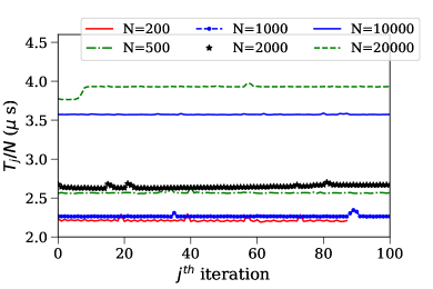
(a) Single core pivot search.

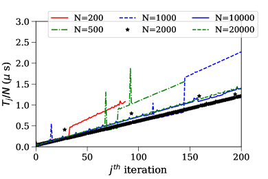
(b) Single core orthogonalization.

Fig. 1: Left: Pivot search time as a function of iteration index $j$. Based solely on operation counts one should expect $T_{j}^{\rm pivot}/N$ to be independent of $N$. Differences are likely due to data access latencies which do depend on $N$. Right: Orthogonalization time as a function of iteration index $j$. As expected, these quantities exhibit a linear growth with $j$. Timing data from the two smallest values of $N$ “jump” due to additional orthogonalization iterations ($\nu$ increases from $1$ to $2$).

6.1.3 Parallel code

We consider a natural parallelization-by-column strategy. Each core  is given a subset of columns to manage, and a separate “master” core is responsible for all orthogonalization activities. We denote $P_{\rm pivot}$ as the number of cores devoted to the pivot search and $P_{\rm ortho}$ as the number of cores devoted to basis orthogonalization. Load balancing is trivially accomplished by distributing $N/P_{\rm pivot}$ columns of $S$ among $P_{\rm pivot}$ cores. Each pivot core loads or creates its chunk of $S$ in parallel. Parallelization of the orthogonalization portion of the algorithm will be discussed later; for now $P_{\rm ortho}=1$.

The $j^{th}$ iteration is initiated after the orthgonalization core broadcasts the $j-1$ basis vector to all $P_{\rm pivot}$ cores. Next, each pivot core computes its contribution of Eq. (6.3) and its maximum. This information is communicated to all pivot and orthgonalization cores. The pivot core with the global maximum residual error sends its column to the orthogonalization core to orthogonalize.

We model the $j^{th}$ iteration’s computational cost as

$$T_{j}=T_{j}^{\rm pivot}+T_{j}^{\rm IMGS}+C_{j}\,,$$ (6.4)

where $T_{j}^{\rm IMGS}$ measures the orthogonalization time, $T_{j}$ is the entire while loop appearing in Alg. 3, and $C_{j}$ includes additional parallelization overheads such as any communication cost and/or thread-management overheads. As equality holds to at worst $1\%$ (typically $0.001\%$), we often report only $T_{j}^{\rm pivot}+C_{j}$ and $T_{j}$. All timing measurements are made from the master process, and the timer measuring $T_{j}^{\rm pivot}$ starts before the next basis vector is broadcasted to all the workers and ends after the next $j+1$ (unorthogonalized) column basis has been received by the master process. Similar to the single core case (cf. Fig. 1(a)) we observe (as expected) $T_{j}^{\rm pivot}+C_{j}$ to be independent of $j$ and, therefore, often report values at some fixed value of $j$.

We consider parallelization by message passing interface (MPI) and OpenMP.

MPI. Each MPI process runs on a unique core. The pivot and orthogononalization cores communicate global pivot information using MPI_Allreduce(), the selected column vector is passed to the orthgonalization work using MPI_Send() and MPI_BCast() provides all the pivot cores with this new orthonormal basis .

OpenMP. OpenMP uses threads to parallelize a portion of the code using the fork-join model. When using OpenMP, we define a large parallel region construct using $P_{\rm pivot}$ threads and enclosing the entire while loop; in fact most of the worker’s code is inside of the parallel region. We found this to given better performance results as compared with parallelizing the for-loop over columns, possibly because a wider parallelized region avoids multiple fork-joins. A designated master thread carries out the orthogonalization task.

Figure 2 considers a family of strong scaling tests where the matrix size is fixed and we vary the number of cores from $1$ to $24$. The left panel reports the parallelization efficiency

$$E_{C}=\frac{T_{1}}{CT_{C}}\,,$$ (6.5)

for the pivot search parallelized with OpenMP, where $C$ is the number of cores, and $T_{1}$ and $T_{C}$ denote the walltime using $1$ and $C$ cores, respectively. Perfect scalability is achieved whenever $E_{C}=1$. The code’s speedup, another often quoted scalability measure, is simply $S_{C}=C\times E_{C}$.

Consistently high efficiencies are observed over a range of problem sizes, with speedups $\approx 20$ routinely observed. For smaller problem sizes, the efficiency is reduced as the parallel overhead $C_{j}$ becomes a sizable fraction of the overall cost . Figure 2(a) shows the pivot search portion of the algorithm is efficiently parallelized. Figure 2(b) shows the full algorithm’s efficiency. Evidently scalability is poor for shorter matrices (small values of $N$), which should be expected from Eq. (6.4) and Amdahl’s law. Approximating the computational cost to be proportional to the asymptotic FLOP count and assuming $M\gg k$, $M>P_{\rm pivot}k$ and $C_{j}=0$, the efficiency of our algorithm is

$$E\approx 1-\nu k(P_{\rm pivot}-1)/(2M)\,.$$ (6.6)

Thus, for good scalability, our problem should require large values of $M$. Most model reduction applications easily meet this requirement. Indeed, model reduction seeks to approximate the underlying continuum problem (often with high parametric dimensionality) for which $M\rightarrow\infty$, while for parametrically smooth models $\sigma_{k}\propto\exp(-k)$. Together, these features suggest $M\gg kP_{\rm pivot}$ is often satisfied in practice.

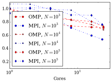
(a) Pivot search portion.

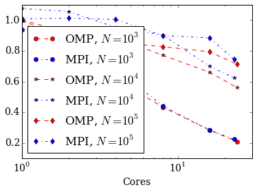
(b) Entire algorithm.

Fig. 2: Strong scaling efficiency versus cores for a sequence of increasingly “tall” matrices with $M=1,000$ and $k=100$ fixed. Our tests were performed on a $24$-core shared memory node of the supercomputer Comet. Blocks of columns are distributed to each core with increasingly fewer blocks per core. Specifically $1000$, $500$, $250$, $125$, $62$, and $43$ columns are distributed among, respectively, $1$, $2$, $4$, $8$, $16$ and $24$ cores. We measure scalability for the pivot search portion (from the timing data $T_{\rm pivot}$) of the algorithm (left) and the full algorithm (right).

6.1.4 Large-core scaling

Our approach to distributed memory parallelization closely follows that of shared memory parallelization. As OpenMP does not support distributed memory environments we cannot use this library for inter-node communication. We consider two cases. First, a pure-MPI parallelization exactly as described in Sec. 6.1.3. Second, a hybrid MPI/OpenMP implementation launching one MPI process per socket . In turn, each MPI process spawns a team OpenMP threads. Each thread is responsible for a matrix chunk over which a local pivot search is performed. As before we avoid multiple thread fork-joins by enclosing the entirety of the while-loop within an OpenMP parallel region, with the master thread responsible for all MPI calls (a so-called “funneled” hybrid approach). As only processes participate in inter-node communication, a hybrid code potentially reduces the communication overhead as compared to a pure-MPI implementation. These benefits could become increasingly important at extremely large core counts.

Figure 3 reports on a few scalability tests we ran on Comet. First, we consider how the pivot search portion of the algorithm scales to large core counts for a fixed matrix size. Figure 3(a) shows a typical case. We see that going from one core to one node maintains high efficiencies, which should be expect in light of Fig. 2(a). Running on an increasing number of cores means each cores has less work to do (fewer columns per core) while the entire algorithm has more communication. As expected, the efficiency decreases but maintains high values up to $370$ cores. Such observations are matrix-dependent, and larger (smaller) matrices are expected to exhibit better (worst) scalability. Interestingly, the MPI/OpenMPI hybrid strategy performs much better than pure-MPI for this problem, indicating that the communication overhead can be somewhat ameliorated; this is also a matrix-dependent observation. Next, we consider how the entire algorithm scales to large core counts when the matrix size is also increased commensurate to the number of core; this constitutes a weak scaling test. Figure 3(b) shows a typical case. We see that the full program’s runtime has negligible increase when going from one core to $1,728$ cores (the maximum allowable size on Comet). This demonstrates that very large matrices can be efficiently handled.

As a final demonstration of our code’s capabilities, we repeat the weak scaling test on Blue Waters where more cores can be used. Figure. 4 shows the same excellent weak scalability all the way up to $32,768$ cores. In particular, we perform a column pivoted QR decomposition (to discover the first $k=100$ basis) on a $10,000$-by-$3,276,800$ sized matrix in $13.5$ seconds. For comparison, it took a similar time of $11.5$ seconds to QR decompose a much smaller $10,000$-by-$3,200$ matrix using $32$ cores.

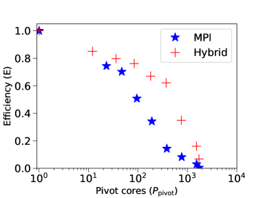
(a) Strong scaling.

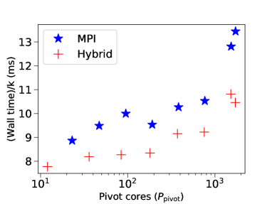
(b) Weak scaling.

Fig. 3: Scalability on the supercomputer Comet up to $1,728$ cores with $k=100$. Left: Strong scaling efficiency of the pivot search part of the algorithm for a matrix with $N=1,000$ rows and $M=240,000$ columns. At $1728$ cores, each pivot core has $\approx 138$ columns and the MPI (Hybrid) efficiency is $.005$ ($.07$), corresponding to very small speedups. This is expected; at this scale the communication time is a sizable fraction of the overall cost, and only increasing the workload (more rows or columns) would increase the efficiency. For this particular matrix size, using $370$ cores the hybrid parallelization strategy has good efficiencies of about $.62$. Of particular importance is that the hybrid code is significantly more efficient than the pure-MPI code. Right: Weak scaling efficiency of the full algorithm for a matrix with $N=10,000$ rows and $M=P_{\rm pivot}\times 100$ columns. The total time is scaled by $k=100$. The slow growth in the total time with increasingly more cores/columns demonstrates good weak scalability, allowing very large matrices to be tackled. (perfect weak scalability would result in a horizontal line.)

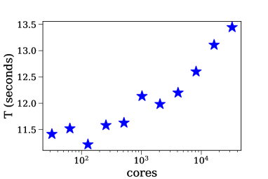
Fig. 4: Weak scaling on Blue Waters with $N=10,000$ rows and $k=100$. We let the number of columns $M=100*{\rm cores}$ scale linearly with the number of cores. The number of cores is increased from $32$ to $32,768$, with the largest matrix having $3,276,800$ columns. A mild logarithmic growth in the full algorithm’s time is evident, and the good weak scalability demonstrates the ability to compute column pivoted QR decompositions of extremely large matrices.

6.1.5 Discussion and Limitations

We have demonstrated our code is capable of handling very large matrix sizes. For smaller sized matrices, the orthogonalization routine becomes a performance obstacle. Because the basis is revealed sequentially, certain efficient algorithms (such as block QR) are not applicable [22]. Furthermore, for conditioning purposes, we have used the IMGS of Hoffman which cannot be written as a matrix-vector product when the basis are sequentially known, thereby precluding efficient BLAS-2 routines [22]. Briefly, we offer three potential solutions. First, alternative orthogonalization algorithms, like the “CMGSI” algorithm of Hoffman may be better suited for parallelization [28]. Second, specialized accelerator hardware may reduce the vector-vector product costs by offloading. Finally, one could consider alternative global pivot selection criteria by overlapping the pivot search and orthogonalization computations.

7 Concluding remarks

Dimensional and model-order reduction have a wide range of applications. In this paper, we have considered two of the most popular dimensional-reduction algorithms, SVD and QR decompositions, and summarized their most important properties. In most model-based dimensional reduction applications the model varies smoothly with parameter variation. In such cases, matrices like the Kahan one are rarely (if ever) encountered in practice. Instead, the approximation problem is characterized by a fast decaying Kolmogorov $n$-width. Due to the equivalence we showed between the RB-Greedy algorithm and a certain QR pivoting strategies, we argue that, for many cases, a QR-based model reduction approach is preferable to an SVD-based one. The QR decomposition is faster and more easily parallelized while providing comparable approximation errors.

Finally, we have described a new, publicly-available QR-based model reduction code, greedycpp [1]. Our code is based on a well-conditioned version of the MGS algorithm which overcomes the stability issues which plague ordinary GS while being straightforward to parallelize (as compared to Householder reflections or Givens rotations). This massively parallel code, developed with model reduction in mind, performed QR decomposition on matrices as large as $10,000$-by-$3,276,800$ on the supercomputers Comet and Blue Waters. Parts of this code have been used to accelerate gravitational wave inference problems [37, 12, 2, 3].

References

- [1] https://bitbucket.org/sfield83/greedycpp.
- [2] BP Abbott, R Abbott, TD Abbott, MR Abernathy, F Acernese, K Ackley, C Adams, T Adams, P Addesso, RX Adhikari, et al., First search for gravitational waves from known pulsars with advanced ligo, The Astrophysical Journal, 839 (2017), p. 12.
- [3] Benjamin P Abbott, R Abbott, TD Abbott, F Acernese, K Ackley, C Adams, T Adams, P Addesso, RX Adhikari, VB Adya, et al., Gw170814: A three-detector observation of gravitational waves from a binary black hole coalescence, Physical Review Letters, 119 (2017), p. 141101.
- [4] , Gw170817: observation of gravitational waves from a binary neutron star inspiral, Physical Review Letters, 119 (2017), p. 161101.
- [5] B. P. Abbott and et al., Gw170104: Observation of a 50-solar-mass binary black hole coalescence at redshift 0.2, Phys. Rev. Lett., 118 (2017), p. 221101.
- [6] H. Antil, S. E. Field, F. Herrmann, R. H. Nochetto, and M. Tiglio, Two-step greedy algorithm for reduced order quadratures, J. Sci. Comput., 57 (2013), pp. 604–637.
- [7] P. Binev, A. Cohen, W. Dahmen, R. DeVore, G. Petrova, and P. Wojtaszczyk, Convergence rates for greedy algorithms in reduced basis methods, SIAM J. Math. Anal., 43 (2011), pp. 1457–1472.
- [8] C. H. Bischof, A parallel qr factorization algorithm with controlled local pivoting, SIAM Journal on Scientific and Statistical Computing, 12 (1991), pp. 36–57.
- [9] Ȧ. Björck, Solving linear least squares problems by Gram-Schmidt orthogonalization, Nordisk Tidskr. Informations-Behandling, 7 (1967), pp. 1–21.
- [10] A. Buffa, Y. Maday, A. T. Patera, C. Prud’homme, and G. Turinici, A priori convergence of the greedy algorithm for the parametrized reduced basis method, ESAIM Math. Model. Numer. Anal., 46 (2012), pp. 595–603.
- [11] P. Businger and G. H. Golub, Handbook series linear algebra. Linear least squares solutions by Householder transformations, Numer. Math., 7 (1965), pp. 269–276.
- [12] P. Canizares, S. E. Field, J. Gair, V. Raymond, R. Smith, and M. Tiglio, Accelerated gravitational wave parameter estimation with reduced order modeling, Physical review letters, 114 (2015), p. 071104.
- [13] T. F. Chan, Rank revealing factorizations, Linear Algebra Appl., 88/89 (1987), pp. 67–82.
- [14] T. F. Chan and P. C. Hansen, Some applications of the rank revealing factorization, SIAM J. Sci. Statist. Comput., 13 (1992), pp. 727–741.
- [15] S. Chandrasekaran and I. C. F. Ipsen, On rank-revealing factorisations, SIAM J. Matrix Anal. Appl., 15 (1994), pp. 592–622.
- [16] S. Chaturantabut and D. C. Sorensen, Nonlinear model reduction via discrete empirical interpolation, SIAM Journal on Scientific Computing, 32 (2010), pp. 2737–2764.
- [17] P. G. Constantine, D. F. Gleich, Y. Hou, and J. Templeton, Model reduction with mapreduce-enabled tall and skinny singular value decomposition, SIAM Journal on Scientific Computing, 36 (2014), pp. S166–S191.
- [18] J. W. Demmel, L. Grigori, M. Gu, and H. Xiang, Communication avoiding rank revealing QR factorization with column pivoting, SIAM J. Matrix Anal. Appl., 36 (2015), pp. 55–89.
- [19] R. DeVore, G. Petrova, and P. Wojtaszczyk, Greedy algorithms for reduced bases in Banach spaces, Constr. Approx., 37 (2013), pp. 455–466.
- [20] Z. Drmač and Z. Bujanović, On the failure of rank-revealing QR factorization software—a case study, ACM Trans. Math. Software, 35 (2009), pp. Art. 12, 28.
- [21] S. E. Field, C. R. Galley, and E. Ochsner, Towards beating the curse of dimensionality for gravitational waves using reduced basis, Physical Review D, 86 (2012), p. 084046.
- [22] E. Gallopoulos, B. Philippe, and A. H. Sameh, Parallelism in matrix computations, Scientific Computation, Springer, Dordrecht, 2016.
- [23] L. Giraud, J. Langou, M. Rozložník, and J. van den Eshof, Rounding error analysis of the classical Gram-Schmidt orthogonalization process, Numer. Math., 101 (2005), pp. 87–100.
- [24] G. Golub, Numerical methods for solving linear least squares problems, Numer. Math., 7 (1965), pp. 206–216.
- [25] G. H. Golub and C. F. Van Loan, Matrix computations, Johns Hopkins Studies in the Mathematical Sciences, Johns Hopkins University Press, Baltimore, MD, third ed., 1996.
- [26] G. Hager and G. Wellein, Introduction to high performance computing for scientists and engineers, CRC Press, 2010.
- [27] M. Hannam, P. Schmidt, A. Bohé, L. Haegel, S. Husa, F. Ohme, G. Pratten, and M. Pürrer, Simple model of complete precessing black-hole-binary gravitational waveforms, Phys. Rev. Lett., 113 (2014), p. 151101.
- [28] W. Hoffmann, Iterative algorithms for Gram-Schmidt orthogonalization, Computing, 41 (1989), pp. 335–348.
- [29] Y. P. Hong and C.-T. Pan, Rank-revealing factorizations and the singular value decomposition, Math. Comp., 58 (1992), pp. 213–232.
- [30] S. Husa, S. Khan, M. Hannam, M. Pürrer, F. Ohme, X. J. Forteza, and A. Bohé, Frequency-domain gravitational waves from nonprecessing black-hole binaries. I. New numerical waveforms and anatomy of the signal, Phys. Rev., D93 (2016), p. 044006.
- [31] S. Khan, S. Husa, M. Hannam, F. Ohme, M. Pürrer, X. J. Forteza, and A. Bohé, Frequency-domain gravitational waves from nonprecessing black-hole binaries. II. A phenomenological model for the advanced detector era, Phys. Rev., D93 (2016), p. 044007.
- [32] Y. Maday, N. .C Nguyen, A. T. Patera, and S. H. Pau, A general multipurpose interpolation procedure: the magic points, Communications on Pure and Applied Analysis, 8 (2009), pp. 383–404.
- [33] Jeroen Meidam, Ka Wa Tsang, Janna Goldstein, Michalis Agathos, Archisman Ghosh, Carl-Johan Haster, Vivien Raymond, Anuradha Samajdar, Patricia Schmidt, Rory Smith, et al., Parametrized tests of the strong-field dynamics of general relativity using gravitational wave signals from coalescing binary black holes: Fast likelihood calculations and sensitivity of the method, Physical Review D, 97 (2018), p. 044033.
- [34] A. Pinkus, N-widths in Approximation Theory, Springer-Verlag, 1985.
- [35] G. Quintana-Ortí and E. S. Quintana-Ortí, Parallel Algorithms for Computing Rank-Revealing QR Factorizations, Springer Berlin Heidelberg, Berlin, Heidelberg, 1997, pp. 122–137.
- [36] A. Ruhe, Numerical aspects of gram-schmidt orthogonalization of vectors, Linear Algebra and its Applications, 52–53 (1983), pp. 591 Р601.
- [37] R. Smith, S. E. Field, K. Blackburn, C.-J. Haster, M. Pürrer, V. Raymond, and P. Schmidt, Fast and accurate inference on gravitational waves from precessing compact binaries, Physical Review D, 94 (2016), p. 044031.
- [38] D. B. Szyld, The many proofs of an identity on the norm of oblique projections, Numer. Algorithms, 42 (2006), pp. 309–323.
- [39] L. N. Trefethen and D. Bau, III, Numerical linear algebra, Society for Industrial and Applied Mathematics (SIAM), Philadelphia, PA, 1997.
- [40] J. A. Tropp, Column subset selection, matrix factorization, and eigenvalue optimization, in Proceedings of the Twentieth Annual ACM-SIAM Symposium on Discrete Algorithms, Society for Industrial and Applied Mathematics, 2009, pp. 978–986.
- [41] J. Xu and L. Zikatanov, Some observations on Babuška and Brezzi theories, Numer. Math., 94 (2003), pp. 195–202.