Present and projected sensitivities of Dark Matter direct detection experiments to effective WIMP-nucleus couplings

Sunghyun Kang francis735@naver.com Stefano Scopel scopel@sogang.ac.kr Gaurav Tomar tomar@sogang.ac.kr Jong–Hyun Yoon jyoon@sogang.ac.kr Department of Physics, Sogang University, Seoul, Korea, 121-742
Abstract

RDD_constraints },
  a simple interpolating code written in Python
  that allows to obtain the numerical value of the bound as a function
  of the WIMP mass $m_{\chi}$ and of the coupling ratio $c^n/c^p$ for
  each 
R coupling. We find that 9 experiments out of the 14 present Dark Matter searches considered in our analysis provide the most stringent bound on some of the effective couplings for a given choice of $(m_{\chi},c^{n}/c^{p})$: this is evidence of the complementarity of different target nuclei and/or different combinations of count–rates and energy thresholds when the search of DM is extended to a wide range of possible interactions.

keywords:
PACS:
95.35.+d ,
††journal: Astroparticle Physics

RDD_constraints },
a simple interpolating code written in Python
that allows to obtain the numerical value of the most constraining
limit on the effective cross section defined in
Eq.(\ref{eq:conventional_sigma_nucleon}) as a function of the WIMP
mass $m_{\chi}$ and of the coupling ratio $c^n/c^p$ for each 
R coupling.

In the present analysis we discuss one of the NR couplings at a time because they are the most general building blocks of the low–energy limit of any ultraviolet theory, so that an understanding of the behaviour of such couplings is crucial for the interpretation of more general scenarios containing the sum of several NR operators222Nevertheless, it is always possible to conceive a linear combination of relativistic operators leading to a single NR operator, since the number of the former is larger than that of the latter, although this might require a tuning of the couplings. . However, our results can be used also to estimate an approximate upper bound on the cross section in the case of the presence of more than one NR operator. The procedure to do so is discussed in Section LABEL:sec:mixing. Our analysis is somewhat complementary to that of Ref.Β [Schneck_eft], where present WIMP direct detection experimental sensitivities are discussed for a limited number of non–relativistic operators and nuclear targets, but interferences among different operators are included in the discussion.

The paper is organized as follows. In Section LABEL:sec:eft we summarize the non–relativistic Effective Field Theory (EFT) approach of Refs.[haxton1, haxton2] and the formulas we use to calculate expected rates for WIMP–nucleus scattering; Section 2 is devoted to our quantitative analysis; in Section LABEL:sec:mixing we show how our results can be applied to the case of more than one NR operator. We will provide our conclusions in Section LABEL:sec:conclusions. In LABEL:app:wimp_eft we provide for completeness the WIMP response functions for the non–relativistic effective theory while in LABEL:app:exp we provide the details of each experiment included in the analysis. LABEL:app:nuclear_response_functions describes our treatment of the nuclear response functions for those isotopes for which a full calculation is not available in the literature. Finally, inΒ LABEL:app:program we introduce

RDD_constraints }, a simple
interpolating code written in Python that allows to retrieve the
numerical value of the limits on the effective WIMP--nucleon cross
section discussed in Section \ref{sec:analysis} and whose contour
plots are shown in Figs.~\ref{fig:c1_plane}--\ref{fig:c15_plane}.
\section{Summary of WIMP rates in non--relativistic effective models}
\label{sec:eft}
Making use of the non--relativistic EFT approach of
Refs. \cite{haxton1,haxton2} the most general Hamiltonian density
describing the WIMP--nucleus interaction can be written as:
\begin{eqnarray}
{\bf\mathcal{H}}({\bf{r}})&=& \sum_{\tau=0,1} \sum_{j=1}^{15} c_j^{\tau} \mathcal{O}_{j}({\bf{r}}) \, t^{\tau} ,
\label{eq:H}
\end{eqnarray}
\noindent where:
\begin{eqnarray}
  \CO_1 &=& 1_\chi 1_
;      O_2 = (v^βŸ‚)^2;      O_3 = i β†’S_N β‹…(β†’qmN Γ—β†’v^βŸ‚);
O_4 &= β†’S_Ο‡β‹…β†’S_N;     O_5 = i β†’S_Ο‡β‹…(β†’qmN Γ—β†’v^βŸ‚);     O_6= (β†’S_Ο‡β‹…β†’qmN) (β†’S_N β‹…β†’qmN) ;
O_7 = β†’S_N β‹…β†’v^βŸ‚;    O_8 = β†’S_Ο‡β‹…β†’v^βŸ‚;    O_9 = i β†’S_Ο‡β‹…(β†’S_N Γ—β†’qmN);
O_10 = i β†’S_N β‹…β†’qmN;    O_11 = i β†’S_Ο‡β‹…β†’qmN;    O_12 = β†’S_Ο‡β‹…(β†’S_N Γ—β†’v^βŸ‚);
O_13 =i (β†’S_Ο‡β‹…β†’v^βŸ‚) ( β†’S_N β‹…β†’qmN);    O_14 = i ( β†’S_Ο‡β‹…β†’qmN)( β†’S_N β‹…β†’v^βŸ‚);
O_15 = - ( β†’S_Ο‡β‹…β†’qmN) ((β†’S_N Γ—β†’v^βŸ‚) β‹…β†’qmN).

In the above equation $1_{\chi N}$ is the identity operator, $\vec{q}$ is the transferred momentum, $\vec{S}_{\chi}$ and $\vec{S}_{N}$ are the WIMP and nucleon spins, respectively, while $\vec{v}^{\perp}=\vec{v}+\frac{\vec{q}}{2\mu_{\chi{\cal N}}}$ (with $\mu_{\chi{\cal N}}$ the WIMP–nucleon reduced mass) is the relative transverse velocity operator satisfying $\vec{v}^{\perp}\cdot\vec{q}=0$. Following Refs.[haxton1, haxton2] in the following we will not include the operator ${\cal O}_{2}$ in our analysis. For a nuclear target $T$ the quantity $(v^{\perp}_{T})^{2}\equiv|\vec{v}^{\perp}_{T}|^{2}$ can also be written as:

$$(v^{\perp}_{T})^{2}=v^{2}_{T}-v_{min}^{2}.$$ (3)

where:

$$v_{min}^{2}=\frac{q^{2}}{4\mu_{T}^{2}}=\frac{m_{T}E_{R}}{2\mu_{T}^{2}},$$ (4)

represents the minimal incoming WIMP speed required to impart the nuclear recoil energy $E_{R}$, while $v_{T}\equiv|\vec{v}_{T}|$ is the WIMP speed in the reference frame of the nuclear center of mass, $m_{T}$ the nuclear mass and $\mu_{T}$ the WIMP–nucleus reduced mass. Moreover $t^{0}=1$, $t^{1}=\tau_{3}$ denote the $2\times 2$ identity and third Pauli matrix in isospin space, respectively, and the isoscalar and isovector (dimension -2) coupling constants $c^{0}_{j}$ and $c^{1}_{j}$, are related to those to protons and neutrons $c^{p}_{j}$ and $c^{n}_{j}$ by $c^{p}_{j}=(c^{0}_{j}+c^{1}_{j})$ and $c^{n}_{j}=(c^{0}_{j}-c^{1}_{j})$.

In the following we will only consider a contact effective interaction between the WIMP and the nucleus, i.e., we will assume the coefficients $c_{j}^{\tau}$ as independent on the transferred momentum $q$. However when the latter is comparable to the pion mass a pole is known to arise in the case of pseudoscalar and axial interactions [bishara]. This may affect our estimation of the sensitivity by less than an order of magnitude for operators ${\it O}_{6}$ and ${\it O}_{10}$ when the WIMP and the target mass are heavy (specifically, for xenon in XENON1T and PANDAX–II and for iodine in PICO-60). Since such effect depends on the particular relativistic model the NR theory descends fromΒ [sogang_eft_rev] and its impact is anyway limited, we have neglected it in our analysis.

The expected rate in a given visible energy bin $E_{1}^{\prime}\leq E^{\prime}\leq E_{2}^{\prime}$ of a direct detection experiment is given by:

$\displaystyle R_{[E_{1}^{\prime},E_{2}^{\prime}]}$ $\displaystyle=$ $\displaystyle M\mbox{T}\int_{E_{1}^{\prime}}^{E_{2}^{\prime}}\frac{dR}{dE^{\prime}}\,dE^{\prime},$ (5)
$\displaystyle\frac{dR}{dE^{\prime}}$ $\displaystyle=$ $\displaystyle\sum_{T}\int_{0}^{\infty}\frac{dR_{\chi T}}{dE_{ee}}{\cal G}_{T}(E^{\prime},E_{ee})\epsilon(E^{\prime})\,dE_{ee},$ (6)
$\displaystyle E_{ee}$ $\displaystyle=$ $\displaystyle q(E_{R})E_{R},$ (7)

with $\epsilon(E^{\prime})\leq 1$ the experimental efficiency/acceptance. In the equations above $E_{R}$ is the recoil energy deposited in the scattering process (indicated in keVnr), while $E_{ee}$ (indicated in keVee) is the fraction of $E_{R}$ that goes into the experimentally detected process (ionization, scintillation, heat) and $q(E_{R})$ is the quenching factor, ${\cal G_{T}}(E^{\prime},E_{ee}=q(E_{R})E_{R})$ is the probability that the visible energy $E^{\prime}$ is detected when a WIMP has scattered off an isotope $T$ in the detector target with recoil energy $E_{R}$, $M$ is the fiducial mass of the detector and T the live–time of the data taking. For a given recoil energy imparted to the target the differential rate for the WIMP–nucleus scattering process is given by:

$$\frac{dR_{\chi T}}{dE_{R}}(t)=\sum_{T}N_{T}\frac{\rho_{\mbox{\tiny WIMP}}}{m_{\chi}}\int_{v_{min}}d^{3}v_{T}f(\vec{v}_{T},t)v_{T}\frac{d\sigma_{T}}{dE_{R}},$$ (8)

where $\rho_{\mbox{\tiny WIMP}}$ is the local WIMP mass density in the neighborhood of the Sun, $N_{T}$ the number of the nuclear targets of species $T$ in the detector (the sum over $T$ applies in the case of more than one nuclear isotope), while

$$\frac{d\sigma_{T}}{dE_{R}}=\frac{2m_{T}}{4\pi v_{T}^{2}}\left[\frac{1}{2j_{\chi}+1}\frac{1}{2j_{T}+1}|\mathcal{M}_{T}|^{2}\right],$$ (9)

and, assuming that the nuclear interaction is the sum of the interactions of the WIMPs with the individual nucleons in the nucleus:

$$\frac{1}{2j_{\chi}+1}\frac{1}{2j_{T}+1}|\mathcal{M}_{T}|^{2}=\frac{4\pi}{2j_{T}+1}\sum_{\tau=0,1}\sum_{\tau^{\prime}=0,1}\sum_{k}R_{k}^{\tau\tau^{\prime}}\left[c^{\tau}_{j},(v^{\perp}_{T})^{2},\frac{q^{2}}{m_{N}^{2}}\right]W_{Tk}^{\tau\tau^{\prime}}(y).$$ (10)

In the above expression $j_{\chi}$ and $j_{T}$ are the WIMP and the target nucleus spins, respectively, $q=|\vec{q}|$ while the $R_{k}^{\tau\tau^{\prime}}$’s are WIMP response functions (that we report for completeness in Eq.(LABEL:eq:wimp_response_functions)) which depend on the couplings $c^{\tau}_{j}$ as well as the transferred momentum $\vec{q}$ and $(v^{\perp}_{T})^{2}$. In equation (10) the $W^{\tau\tau^{\prime}}_{Tk}(y)$’s are nuclear response functions and the index $k$ represents different effective nuclear operators, which, crucially, under the assumption that the nuclear ground state is an approximate eigenstate of $P$ and $CP$, can be at most eight: following the notation in [haxton1, haxton2], $k$=$M$, $\Phi^{\prime\prime}$, $\Phi^{\prime\prime}M$, $\tilde{\Phi}^{\prime}$, $\Sigma^{\prime\prime}$, $\Sigma^{\prime}$, $\Delta$,$\Delta\Sigma^{\prime}$. The $W^{\tau\tau^{\prime}}_{Tk}(y)$’s are function of $y\equiv(qb/2)^{2}$, where $b$ is the size of the nucleus. For the target nuclei $T$ used in most direct detection experiments the functions $W^{\tau\tau^{\prime}}_{Tk}(y)$, calculated using nuclear shell models, have been provided in Refs.Β [haxton2, catena] under the assumption that the dark matter particle couples to the nucleus through local one–body interactions with the nucleons. In our analysis we do not include two–body effectsΒ [two_body_1, two_body_2] which are only available for a few isotopes and can be important when the one–body contribution is suppressed.

In the present paper, we will systematically consider the possibility that one of the couplings $c_{j}$ dominates in the effective Hamiltonian of Eq. (LABEL:eq:H). In this case it is possible to factorize a term $|c_{j}^{p}|^{2}$ from the squared amplitude of Eq.(10) and express it in terms of the effective WIMP–proton cross section333With the definition of Eq.(11) the WIMP–proton SI cross section is equal to $\sigma_{p}$, and the SD WIMP–proton cross section to 3/16 $\sigma_{p}$.:

$$\sigma_{p}=(c_{j}^{p})^{2}\frac{\mu_{\chi{\cal N}}^{2}}{\pi},$$ (11)

(with $\mu_{\chi{\cal N}}$ the WIMP–nucleon reduced mass) and the ratio $r\equiv c_{j}^{n}/c_{j}^{p}$. It is worth pointing out here that among the generalized nuclear response functions arising from the effective Hamiltonian of Eq. (LABEL:eq:H) only the ones corresponding to $M$ (SI interaction), $\Sigma^{\prime\prime}$ and $\Sigma^{\prime}$ (both related to the standard spin–dependent interaction) do not vanish for $q\rightarrow$0, and so allow to interpret $\sigma_{p}$ in terms of a long–distance, point–like cross section. In the case of the other interactions $\Phi^{\prime\prime}$, $\Phi^{\prime\prime}M$, $\tilde{\Phi}^{\prime}$, $\Delta$ and $\Delta\Sigma^{\prime}$ the quantity $\sigma_{p}$ is just a convenient alternative to directly parameterizing the interaction in terms of the $c_{j}^{p}$ coupling.

Finally, $f(\vec{v}_{T})$ is the WIMP velocity distribution, for which we assume a standard isotropic Maxwellian at rest in the Galactic rest frame truncated at the escape velocity $u_{esc}$, and boosted to the Lab frame by the velocity of the Earth. So for the former we assume:

$\displaystyle f(\vec{v}_{T},t)$ $\displaystyle=$ N​(32​π​vr​m​s2)3/2​eβˆ’3​|vβ†’T+vβ†’E|22​vr​m​s2β€‹Ξ˜β€‹(ue​s​cβˆ’|vβ†’T+vβ†’E​(t)|),𝑁superscript32πœ‹superscriptsubscriptπ‘£π‘Ÿπ‘šπ‘ 232superscript𝑒3superscriptsubscript→𝑣𝑇subscript→𝑣𝐸22superscriptsubscriptπ‘£π‘Ÿπ‘šπ‘ 2Θsubscript𝑒𝑒𝑠𝑐subscript→𝑣𝑇subscript→𝑣𝐸𝑑\displaystyle N\left(\frac{3}{2\pi v_{rms}^{2}}\right)^{3/2}e^{-\frac{3|\vec{v}_{T}+\vec{v}_{E}|^{2}}{2v_{rms}^{2}}}\Theta(u_{esc}-|\vec{v}_{T}+\vec{v}_{E}(t)|), (12)
$\displaystyle N$ $\displaystyle=$ $\displaystyle\left[\mbox{erf}(z)-\frac{2}{\sqrt{\pi}}ze^{-z^{2}}\right]^{-1},$ (13)

with z=3​ue​s​c2/(2​vr​m​s2)𝑧3superscriptsubscript𝑒𝑒𝑠𝑐22superscriptsubscriptπ‘£π‘Ÿπ‘šπ‘ 2z=3u_{esc}^{2}/(2v_{rms}^{2}). In the isothermal sphere model hydrothermal equilibrium between the WIMP gas pressure and gravity is assumed, leading to vr​m​ssubscriptπ‘£π‘Ÿπ‘šπ‘ v_{rms}=$\sqrt{3/2}v_{0}$ with $v_{0}$ the galactic rotational velocity.

With the exception of DAMA, all the experiments included in our analysis are sensitive to the time average of the expected rate for which $<v_{E}>$=$v_{\odot}$ and $v_{\odot}$=$v_{0}$+12 (accounting for a peculiar component of the solar system with respect to the galactic rotation). In the case of DAMA, the yearly modulation effect is due to the time dependence of the Earth’s speed with respect to the Galactic frame, given by:

$$|\vec{v}_{E}(t)|=v_{\odot}+v_{orb}\cos\gamma\cos\left[\frac{2\pi}{T_{0}}(t-t_{0})\right],$$ (14)

where $\cos\gamma\simeq$0.49 accounts for the inclination of the ecliptic plane with respect to the Galactic plane, $T_{0}$=1 year and $v_{orb}$=2$\pi r_{\oplus}/(T_{0})\simeq$ 29 km/sec ($r_{\oplus}$=1 AU neglecting the small eccentricity of the Earth’s orbit around the Sun).

In our analysis for the two parameters $v_{0}$ and $u_{esc}$ we take $v_{0}$=220 km/sec [v0_koposov] and $u_{esc}$=550 km/sec [vesc_2014]. Our choice of parameters corresponds to a WIMP escape velocity in the lab rest frame ve​s​cl​a​b≃similar-to-or-equalssuperscriptsubscriptπ‘£π‘’π‘ π‘π‘™π‘Žπ‘absentv_{esc}^{lab}\simeq 782 km/s. To make contact with other analyses, for the dark matter density in the neighborhood of the Sun we use $\rho_{\mbox{\tiny WIMP}}$=0.3, which is a standard value commonly adopted by experimental collaborations, although observations point to the slightly higher value $\rho_{\mbox{\tiny WIMP}}$=0.43 [rho_DM_salucci_1, rho_DM_salucci_2]. Notice that direct detection experiments are only sensitive to the product $\rho_{\mbox{\tiny WIMP}}\sigma_{p}$, so the results of the next Section can be easily rescaled with $\rho_{\mbox{\tiny WIMP}}$.

2 Analysis

Refer to caption
Refer to caption
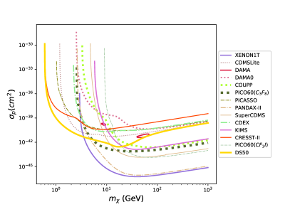
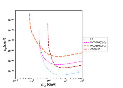
Figure 1: Current (left) and future (right) 90% C.L. exclusion plots to the effective WIMP–proton cross section $\sigma_{p}$ of Eq. (11) for the SI interaction of Eq. (LABEL:eq:si) corresponding to the ${\cal O}_{1}$ operator in Eq.(LABEL:eq:H) for the isoscalar case $c_{1}^{p}$=$c_{1}^{n}$. The figure shows the constraints from the full set of experiments that we include in our analysis, which consists in the latest available data from 14 existing DM searches, and the estimated future sensitivity of 4 projected ones (LZ, PICO-500 (C3F8), PICO-500 (CF3I) and COSINUS). The closed solid (red) contour represents the 5–sigma DAMA modulation amplitude region, while we indicate with DAMA0 the upper bound from the DAMA average count–rate. Notice that after the release of the DAMA/LIBRA-phase2 resultΒ [dama_2018] a spin–independent isoscalar ($c^{n}/c^{p}$=1) interaction does not provide anymore a good fit to the modulation effect, while it still does for different values of $c^{n}/c^{p}$ and for other effective couplings [dama_2018_sogang].

The current 90% C.L. exclusion plots to the effective WIMP–proton cross section $\sigma_{p}$ of Eq. (11) for the SI interaction of Eq.(LABEL:eq:si) (corresponding to the ${\cal O}_{1}$ operator in Eq.(LABEL:eq:H)) are shown for the isoscalar case $c_{1}^{p}$=$c_{1}^{n}$ and for the full set of the DM search experiments that we include in our analysis in Fig.1. The plot includes the latest available data from a total of 14 existing experiments, and the estimated future sensitivity of 4 projected ones. The details of our procedure to obtain the exclusion plots are provided in LABEL:app:exp.

The relative sensitivity of different detectors is determined by two elements: the thresholds $v_{min}^{th}$ of different experiments expressed in terms of the WIMP incoming velocity, and the scaling law of the WIMP–nucleus cross section off different targets.

The former element explains the steep rise of all the exclusion plot curves at low WIMP masses, which corresponds to the case when $v_{min}^{th}$ approaches the value of the escape velocity in the lab rest frame, and is sensitive to experimental features close to the energy threshold that are typically affected by uncertainties, such as efficiencies, acceptances and charge/light yields. With the assumptions listed in LABEL:app:exp, among the experiments included in our analysis the ones with the lowest velocity thresholds turn out to be DS50, CRESST–II, CDMSlite and CDEX. In particular, for $m_{\chi}$=1 GeV we have $v_{min,DS50}^{th}\simeq$ 450 km/s, $v_{min,CRESST-II}^{th}\simeq$ 480 km/s (for scatterings off oxygen), $v_{min,CDMSlite}^{th}\simeq$ 910 km/s, $v_{min,CDEX}^{th}\simeq$ 1600 km/s. Assuming ve​s​cl​a​b≃similar-to-or-equalssuperscriptsubscriptπ‘£π‘’π‘ π‘π‘™π‘Žπ‘absentv_{esc}^{lab}\simeq 782 km/s (see the previous Section) this implies that in our analysis only DS50 and CRESST-II (for effective interactions for which argon and oxygen have a non–vanishing nuclear response function) are sensitive to $m_{\chi}\mathrel{\mathop{\kern 0.0pt\hbox to0.0pt{\raise 0.86108pt\hbox{$<$}\hss}}\lower 3.87495pt\hbox{\kern-1.90002pt$\sim$}}$ 1 GeV. On the other hand CDMSlite and CDEX are sensitive to slightly higher masses (for instance, for $m_{\chi}$=2 GeV $v_{min,CDMSlite}^{th}\simeq$ 460 km/s, $v_{min,CDEX}^{th}\simeq$ 850 km/s, while for $m_{\chi}$=3 GeV $v_{min,CDEX}^{th}\simeq$ 580 km/s). The velocity threshold is a purely kinematical feature that does not depend on the type of interaction and that favors experiments with the lowest $v_{min}^{th}$ at fixed $m_{\chi}$.

With the exception of very low masses, where the effect of $v_{min}^{th}$ is dominant, the relative sensitivity of different detectors is determined by the scaling law of the WIMP–nucleus cross section with different targets, which is the focus of our analysis. In particular the SI interaction (corresponding to the $M$ effective nuclear operator) favors heavy nuclei, so that the most stringent bounds in Fig. 1 correspond to xenon experiments (XENON1T, PANDAX-II). However the interaction terms in the Hamiltonian of Eq.(LABEL:eq:H) lead to expected rates that depend on the full set of possible nuclear operators ($M$, $\Phi^{\prime\prime}$, $\tilde{\Phi}^{\prime}$, $\Sigma^{\prime\prime}$, $\Sigma^{\prime}$, $\Delta$) leading to different scaling laws of the WIMP–nucleus cross section on different targets. The correspondence between models and nuclear response functions can be directly read off from the WIMP response functions $R^{\tau\tau^{\prime}}_{k}$ (see Eq.LABEL:eq:wimp_response_functions). In particular, using the decomposition:

$$R_{k}^{\tau\tau^{\prime}}=R_{0k}^{\tau\tau^{\prime}}+R_{1k}^{\tau\tau^{\prime}}(v^{\perp}_{T})^{2}=R_{0k}^{\tau\tau^{\prime}}+R_{1k}^{\tau\tau^{\prime}}\left(v_{T}^{2}-v_{min}^{2}\right),$$ (15)

such correspondence is summarized in Table 
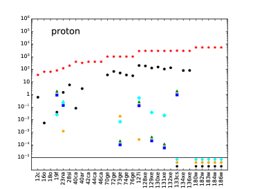
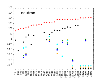
1. In Fig. 2 we provide for completeness the nuclear response functions at vanishing momentum transfer off protons 16​π/(2​jT+1)Γ—WT​kp​(y=0)16πœ‹2subscript𝑗𝑇1subscriptsuperscriptπ‘Šπ‘π‘‡π‘˜π‘¦016\pi/(2j_{T}+1)\times W^{p}_{Tk}(y=0) (left–hand plot) and off neutrons 16​π/(2​jT+1)Γ—WT​kn​(y=0)16πœ‹2subscript𝑗𝑇1subscriptsuperscriptπ‘Šπ‘›π‘‡π‘˜π‘¦016\pi/(2j_{T}+1)\times W^{n}_{Tk}(y=0) (right–hand plot), with WT​kp,n≑1/4Γ—(WT​k00Β±WT​k01Β±WT​k10+WT​k11)subscriptsuperscriptπ‘Šπ‘π‘›π‘‡π‘˜14plus-or-minussubscriptsuperscriptπ‘Š00π‘‡π‘˜subscriptsuperscriptπ‘Š01π‘‡π‘˜subscriptsuperscriptπ‘Š10π‘‡π‘˜subscriptsuperscriptπ‘Š11π‘‡π‘˜W^{p,n}_{Tk}\equiv 1/4\times(W^{00}_{Tk}\pm W^{01}_{Tk}\pm W^{10}_{Tk}+W^{11}_{Tk}) for kπ‘˜k=M𝑀M, Ξ¦β€²β€²superscriptΞ¦β€²β€²\Phi^{\prime\prime}, Ξ¦~β€²superscript~Ξ¦β€²\tilde{\Phi}^{\prime}, Ξ£β€²β€²superscriptΞ£β€²β€²\Sigma^{\prime\prime}, Ξ£β€²superscriptΞ£β€²\Sigma^{\prime}, ΔΔ\Delta and all the targets T𝑇T used in the present analysis, as calculated in [haxton2, catena]. The normalization factor is chosen so that 16​π/(2​jT+1)Γ—WT​Mp​(y=0)16πœ‹2subscript𝑗𝑇1subscriptsuperscriptπ‘Šπ‘π‘‡π‘€π‘¦016\pi/(2j_{T}+1)\times W^{p}_{TM}(y=0)=ZT2superscriptsubscript𝑍𝑇2Z_{T}^{2} and 16​π/(2​jT+1)Γ—WT​Mn​(y=0)16πœ‹2subscript𝑗𝑇1subscriptsuperscriptπ‘Šπ‘›π‘‡π‘€π‘¦016\pi/(2j_{T}+1)\times W^{n}_{TM}(y=0)=(ATβˆ’ZT)2superscriptsubscript𝐴𝑇subscript𝑍𝑇2(A_{T}-Z_{T})^{2} with ATsubscript𝐴𝑇A_{T}, ZTsubscript𝑍𝑇Z_{T} the mass and atomic numbers for target T𝑇T. In the same figure values below the horizontal line at 1Γ—10βˆ’41superscript1041\times 10^{-4} represent nuclear response functions that are missing in the literature. They enter in the calculation of expected rates in KIMS (caesium, using CsI) and CRESST-II (tungsten, using CaWO4). In both cases we have calculated the expected rate on the targets with known nuclear response functions and set to zero the missing ones, so that the corresponding constraints must be considered as conservative estimates. For the targets for which Refs.Β [haxton2, catena] do not provide the nuclear response functions we evaluate the standard SI and SD interactions following the procedure of LABEL:app:nuclear_response_functions.

coupling $R^{\tau\tau^{\prime}}_{0k}$ $R^{\tau\tau^{\prime}}_{1k}$ coupling $R^{\tau\tau^{\prime}}_{0k}$ $R^{\tau\tau^{\prime}}_{1k}$
$1$ $M(q^{0})$ - $3$ $\Phi^{\prime\prime}(q^{4})$ $\Sigma^{\prime}(q^{2})$
$4$ $\Sigma^{\prime\prime}(q^{0})$,$\Sigma^{\prime}(q^{0})$ - $5$ $\Delta(q^{4})$ $M(q^{2})$
$6$ $\Sigma^{\prime\prime}(q^{4})$ - $7$ - $\Sigma^{\prime}(q^{0})$
$8$ $\Delta(q^{2})$ $M(q^{0})$ $9$ $\Sigma^{\prime}(q^{2})$ -
$10$ $\Sigma^{\prime\prime}(q^{2})$ - $11$ $M(q^{2})$ -
$12$ $\Phi^{\prime\prime}(q^{2})$,$\tilde{\Phi}^{\prime}(q^{2})$ $\Sigma^{\prime\prime}(q^{0})$,$\Sigma^{\prime}(q^{0})$ $13$ $\tilde{\Phi}^{\prime}(q^{4})$ $\Sigma^{\prime\prime}(q^{2})$
$14$ - $\Sigma^{\prime}(q^{2})$ $15$ $\Phi^{\prime\prime}(q^{6})$ $\Sigma^{\prime}(q^{4})$
Table 1: Nuclear response functions corresponding to each coupling, for the velocity–independent and the velocity–dependent components parts of the WIMP response function, decomposed as in Eq.(15). In parenthesis the power of $q$ in the WIMP response function.
Refer to caption
Refer to caption
Refer to caption
Figure 2: Nuclear response functions at vanishing momentum transfer off protons $16\pi/(2j_{T}+1)\times W^{p}_{Tk}(y=0)$ (left–hand plot) and off neutrons $16\pi/(2j_{T}+1)\times W^{n}_{Tk}(y=0)$ (right–hand plot), for $k$=$M$, $\Phi^{\prime\prime}$, $\tilde{\Phi}^{\prime}$, $\Sigma^{\prime\prime}$, $\Sigma^{\prime}$, $\Delta$ and all the targets $T$ used in the present analysis. The normalization factor is chosen so that $16\pi/(2j_{T}+1)\times W^{p}_{TM}(y=0)$=$Z_{T}^{2}$ and $16\pi/(2j_{T}+1)\times W^{n}_{TM}(y=0)$=$(A_{T}-Z_{T})^{2}$ with $A_{T}$, $Z_{T}$ the mass and atomic numbers for target $T$. Markers below the horizontal solid line represent nuclear response functions that are missing in the literature. In our analysis we have set them to zero.

The sensitivity of present experiments to each of the couplings of the effective Hamiltonian of Eq.(LABEL:eq:H) is discussed in Figs. LABEL:fig:c1_plane–LABEL:fig:c15_plane, which show the contour plots of the most stringent 90% C.L. bound on the effective WIMP–nucleon cross section $\sigma_{\cal N}$, defined as:

$$\sigma_{\cal N}=\max(\sigma_{p},\sigma_{n}),$$ (16)

as a function of the WIMP mass $m_{\chi}$ and of the ratio $c^{n}/c^{p}$ between the WIMP–neutron and the WIMP–proton couplings. The numerical values in the figures indicate the most stringent bound on $\sigma_{\cal N}$ in cm2. In each plot the different shadings (colors) indicate the experiment providing the most constraining bound, as indicated in the corresponding legend. To make such plots of practical use, inΒ LABEL:app:program we introduce

RDD_constraints }, a simple interpolating code written in Python
that allows to extract the numerical values of $\sigma_{\cal 
fromFigs.LABEL:fig:c1_planeβˆ’βˆ’LABEL:fig:c15_plane.Inthecalculationofalltheplotsthelowerpartofthe2βˆ’βˆ’sigmaDAMAmodulationamplituderegioninthefromFigs.~{}\ref{fig:c1_plane}--\ref{fig:c15_plane}.Inthecalculationofalltheplotsthelowerpartofthe2--sigmaDAMAmodulationamplituderegioninthem_Ο‡βˆ’β£βˆ’--Οƒ_pplaneisincludedasifitwereanadditionalconstraint,inordertolocatepossibleregionsofcompatibilitybetweentheDAMAexcessandotherconstraintsintheparameterspace.AscanbeseenfromFigs.LABEL:fig:c1_planeβˆ’βˆ’LABEL:fig:c15_planeDAMAneverappearsasthemostconstrainingbound,indicatingthatanexplanationofitsannualmodulationexcessintermsofaWIMPsignalisintensionwiththeconstraintsofotherexperimentsnomatterwhichoftheeffectiveoperatorsamongthoseinEq.(LABEL:eq:H)isassumedtodominateintheWIMPβˆ’βˆ’nucleusinteractionandforallplaneisincludedasifitwereanadditionalconstraint,inordertolocatepossibleregionsofcompatibilitybetweentheDAMAexcessandotherconstraintsintheparameterspace.AscanbeseenfromFigs.\ref{fig:c1_plane}--\ref{fig:c15_plane}DAMAneverappearsasthemostconstrainingbound,indicatingthatanexplanationofitsannualmodulationexcessintermsofaWIMPsignalisintensionwiththeconstraintsofotherexperimentsnomatterwhichoftheeffectiveoperatorsamongthoseinEq.(\ref{eq:H})isassumedtodominateintheWIMP--nucleusinteractionandforall(m_Ο‡βˆ’β£βˆ’--Οƒ_N)combinations.ThisresultisinagreementwiththefindingsofRef.[Catena_dama, dama_2018_sogang].ThedifferentpatternsoftheregionsappearinginFigs.LABEL:fig:c1_planeβˆ’βˆ’LABEL:fig:c15_planecanbeunderstoodwiththehelpofTable1andFig.2.Inparticular,thevelocityβˆ’βˆ’dependentcontributionproportionalto)combinations.ThisresultisinagreementwiththefindingsofRef.~{}\cite[cite]{[\@@bibref{Number}{Catena_dama,dama_2018_sogang}{}{}]}.\par ThedifferentpatternsoftheregionsappearinginFigs.\ref{fig:c1_plane}--\ref{fig:c15_plane}canbeunderstoodwiththehelpofTable\ref{table:eft_summary}andFig.\ref{fig:scaling_law}.Inparticular,thevelocity--dependentcontributionproportionalto(v^βŸ‚_T)^2i​s​n​e​g​l​i​g​i​b​l​e​o​r​a​b​s​e​n​t​i​n​a​l​l​c​a​s​e​s​w​i​t​h​5​e​x​c​e​p​t​i​o​n​s::π‘–π‘ π‘›π‘’π‘”π‘™π‘–π‘”π‘–π‘π‘™π‘’π‘œπ‘Ÿπ‘Žπ‘π‘ π‘’π‘›π‘‘π‘–π‘›π‘Žπ‘™π‘™π‘π‘Žπ‘ π‘’π‘ π‘€π‘–π‘‘β„Ž5𝑒π‘₯π‘π‘’π‘π‘‘π‘–π‘œπ‘›π‘ absentisnegligibleorabsentinallcaseswith5exceptions:c_7$and$c_14$(wherethevelocity--independenttermisnotpresent),$c_5$and$c_8$(whereitisenhancedbythe$M$coherentresponsefunctions)andforthecoupling$c_13(s​e​e​b​e​l​o​w).A​s​a​c​o​n​s​e​q​u​e​n​c​e​o​f​t​h​i​s,t​h​e​i​n​t​e​r​a​c​t​i​o​n​t​e​r​m​sformulae-sequenceπ‘ π‘’π‘’π‘π‘’π‘™π‘œπ‘€π΄π‘ π‘Žπ‘π‘œπ‘›π‘ π‘’π‘žπ‘’π‘’π‘›π‘π‘’π‘œπ‘“π‘‘β„Žπ‘–π‘ π‘‘β„Žπ‘’π‘–π‘›π‘‘π‘’π‘Ÿπ‘Žπ‘π‘‘π‘–π‘œπ‘›π‘‘π‘’π‘Ÿπ‘šπ‘ (seebelow).Asaconsequenceofthis,theinteractiontermsc_1,c_5,c_8$and$c_11$dependonthe$M$coherentresponsefunctionwithaconsequentstrongsensitivityofxenondetectors(XENON1TandPANDAX--II)exceptfor$c^n/c^pβ‰ƒβˆ’0.7​c​o​r​r​e​s​p​o​n​d​i​n​g​t​o​a​s​u​p​p​r​e​s​s​i​o​n​o​n​x​e​n​o​n​t​a​r​g​e​t​s.B​y​t​h​e​s​a​m​e​t​o​k​e​n,t​h​e​i​n​t​e​r​a​c​t​i​o​n​s​t​e​r​m​sformulae-sequence0.7π‘π‘œπ‘Ÿπ‘Ÿπ‘’π‘ π‘π‘œπ‘›π‘‘π‘–π‘›π‘”π‘‘π‘œπ‘Žπ‘ π‘’π‘π‘π‘Ÿπ‘’π‘ π‘ π‘–π‘œπ‘›π‘œπ‘›π‘₯π‘’π‘›π‘œπ‘›π‘‘π‘Žπ‘Ÿπ‘”π‘’π‘‘π‘ π΅π‘¦π‘‘β„Žπ‘’π‘ π‘Žπ‘šπ‘’π‘‘π‘œπ‘˜π‘’π‘›π‘‘β„Žπ‘’π‘–π‘›π‘‘π‘’π‘Ÿπ‘Žπ‘π‘‘π‘–π‘œπ‘›π‘ π‘‘π‘’π‘Ÿπ‘šπ‘ -0.7correspondingtoasuppressiononxenontargets.Bythesametoken,theinteractionstermsc_4,c_6,c_7,c_9,c_10$and$c_14d​e​p​e​n​d​o​n​t​h​e​r​e​s​p​o​n​s​e​f​u​n​c​t​i​o​n​sπ‘‘π‘’π‘π‘’π‘›π‘‘π‘œπ‘›π‘‘β„Žπ‘’π‘Ÿπ‘’π‘ π‘π‘œπ‘›π‘ π‘’π‘“π‘’π‘›π‘π‘‘π‘–π‘œπ‘›π‘ dependontheresponsefunctionsΞ£^β€²β€²a​n​d/o​rπ‘Žπ‘›π‘‘π‘œπ‘Ÿand/orΞ£^β€²,thatarerelatedtothespinβˆ’βˆ’dependentcouplingofEq.(LABEL:eq:sd):inparticular,,thatarerelatedtothespin--dependentcouplingofEq.(\ref{eq:sd}):inparticular,Ξ£^β€²β€²c​o​r​r​e​s​p​o​n​d​s​t​o​t​h​e​c​o​u​p​l​i​n​g​o​f​t​h​e​W​I​M​P​t​o​t​h​e​c​o​m​p​o​n​e​n​t​o​f​t​h​e​n​u​c​l​e​o​n​s​p​i​n​a​l​o​n​g​t​h​e​d​i​r​e​c​t​i​o​n​o​f​t​h​e​t​r​a​n​s​f​e​r​r​e​d​m​o​m​e​n​t​u​mπ‘π‘œπ‘Ÿπ‘Ÿπ‘’π‘ π‘π‘œπ‘›π‘‘π‘ π‘‘π‘œπ‘‘β„Žπ‘’π‘π‘œπ‘’π‘π‘™π‘–π‘›π‘”π‘œπ‘“π‘‘β„Žπ‘’π‘ŠπΌπ‘€π‘ƒπ‘‘π‘œπ‘‘β„Žπ‘’π‘π‘œπ‘šπ‘π‘œπ‘›π‘’π‘›π‘‘π‘œπ‘“π‘‘β„Žπ‘’π‘›π‘’π‘π‘™π‘’π‘œπ‘›π‘ π‘π‘–π‘›π‘Žπ‘™π‘œπ‘›π‘”π‘‘β„Žπ‘’π‘‘π‘–π‘Ÿπ‘’π‘π‘‘π‘–π‘œπ‘›π‘œπ‘“π‘‘β„Žπ‘’π‘‘π‘Ÿπ‘Žπ‘›π‘ π‘“π‘’π‘Ÿπ‘Ÿπ‘’π‘‘π‘šπ‘œπ‘šπ‘’π‘›π‘‘π‘’π‘šcorrespondstothecouplingoftheWIMPtothecomponentofthenucleonspinalongthedirectionofthetransferredmomentumβ†’q$while$Ξ£^β€²t​o​t​h​a​t​p​e​r​p​e​n​d​i​c​u​l​a​r​t​o​i​t,w​i​t​hπ‘‘π‘œπ‘‘β„Žπ‘Žπ‘‘π‘π‘’π‘Ÿπ‘π‘’π‘›π‘‘π‘–π‘π‘’π‘™π‘Žπ‘Ÿπ‘‘π‘œπ‘–π‘‘π‘€π‘–π‘‘β„Žtothatperpendiculartoit,withW^ττ^β€²_Ξ£^β€²(q^2)≃2 W^ττ^β€²_Ξ£^β€²β€²(q^2)$when$q^2β†’0$.Sinceinsidenucleithenucleonsspinstendtocanceleachotherthecontributionfromeven--numberednucleonstotheresponsefunctions$Ξ£^β€²β€²a​n​dπ‘Žπ‘›π‘‘andΞ£^β€²isstronglysuppressed.Asaconsequenceofthisforsuchinteractionsneutronβˆ’βˆ’oddtargets(suchasxenonandgermanium)aremostlysensitivetotheregimeisstronglysuppressed.Asaconsequenceofthisforsuchinteractionsneutron--oddtargets(suchasxenonandgermanium)aremostlysensitivetotheregimeβ€”c^n/c^pβ€”>>$\sim$ $1whileproton--oddones(suchasfluorineandiodine)mainlyconstraintheoppositecase$β€”c^n/c^pβ€”<<$\sim$1.T​h​i​s​r​e​f​l​e​c​t​s​i​n​t​h​e​p​a​t​t​e​r​n​o​f​t​h​e​s​h​a​d​e​d​a​r​e​a​s​o​f​F​i​g​s.LABEL:fig:c4_plane,LABEL:fig:c6_plane,LABEL:fig:c7_plane,LABEL:fig:c9_plane,LABEL:fig:c10_plane​a​n​d​LABEL:fig:c14_plane,w​h​e​r​e​f​o​rformulae-sequence1π‘‡β„Žπ‘–π‘ π‘Ÿπ‘’π‘“π‘™π‘’π‘π‘‘π‘ π‘–π‘›π‘‘β„Žπ‘’π‘π‘Žπ‘‘π‘‘π‘’π‘Ÿπ‘›π‘œπ‘“π‘‘β„Žπ‘’π‘ β„Žπ‘Žπ‘‘π‘’π‘‘π‘Žπ‘Ÿπ‘’π‘Žπ‘ π‘œπ‘“πΉπ‘–π‘”π‘ LABEL:fig:c4_planeLABEL:fig:c6_planeLABEL:fig:c7_planeLABEL:fig:c9_planeLABEL:fig:c10_planeπ‘Žπ‘›π‘‘LABEL:fig:c14_planeπ‘€β„Žπ‘’π‘Ÿπ‘’π‘“π‘œπ‘Ÿ1.ThisreflectsinthepatternoftheshadedareasofFigs.\ref{fig:c4_plane},\ref{fig:c6_plane},\ref{fig:c7_plane},\ref{fig:c9_plane},\ref{fig:c10_plane}and\ref{fig:c14_plane},whereform_Ο‡>>$\sim$ $1GeVthePICASSOandPICO(C$_3$F$_8$)bounds(usingproton--oddfluorine)arethemostconstraininglimitsfor$β€”c^n/c^pβ€”<<$\sim$ $1(withtheexceptionof$c_6$,wherealsoPICO(CF$_3$I)becomescompetitiveinspiteoftherelativelylargeenergythreshold($E_R$=13.6keV)duetothe$q

Conversion to HTML had a Fatal error and exited abruptly. This document may be truncated or damaged.