Semi-Blind Inference of Topologies and
Dynamical Processes over Graphs
Abstract
Network science provides valuable insights across numerous disciplines including sociology, biology, neuroscience and engineering. A task of major practical importance in these application domains is inferring the network structure from noisy observations at a subset of nodes. Available methods for topology inference typically assume that the process over the network is observed at all nodes. However, application-specific constraints may prevent acquiring network-wide observations. Alleviating the limited flexibility of existing approaches, this work advocates structural models for graph processes and develops novel algorithms for joint inference of the network topology and processes from partial nodal observations. Structural equation models (SEMs) and structural vector autoregressive models (SVARMs) have well-documented merits in identifying even directed topologies of complex graphs; while SEMs capture contemporaneous causal dependencies among nodes, SVARMs further account for time-lagged influences. This paper develops algorithms that iterate between inferring directed graphs that “best” fit the data, and estimating the network processes at reduced computational complexity by leveraging tools related to Kalman smoothing. To further accommodate delay-sensitive applications, an online joint inference approach is put forth that even tracks time-evolving topologies. Furthermore, conditions for identifying the network topology given partial observations are specified. It is proved that the required number of observations for unique identification reduces significantly when the network structure is sparse. Numerical tests with synthetic as well as real datasets corroborate the effectiveness of the novel approach.
Index Terms:
Graph signal reconstruction, topology inference, directed graphs, structural (vector) equation models.I Introduction
Modeling vertex attributes as processes that take values over a graph allows for data processing tasks, such as filtering, inference, and compression, while accounting for information captured by the network topology [34, 20]. However, if the topology is unavailable, inaccurate or even unrelated to the process of interest, performance of the associated task may degrade severely. For example, consider a social graph where the goal is to predict the salaries of all individuals given the salaries of some. Graph-based inference approaches that assume smoothness of the salary over the given graph, may fall short if the salary is dissimilar among friends.
Topology identification is possible when observations at all nodes are available by employing structural models, see e.g., [18]. However, in many real settings one can only afford to collect nodal observations from a subset of nodes due to application-specific restrictions. For example, sampling all nodes may be prohibitive in massive graphs; in social networks individuals may be reluctant to share personal information due to privacy concerns; in sensor networks, devices may report measurements sporadically to save energy; and in gene regulatory networks, gene expression data may contain misses due to experimental errors. In this context, the present paper relies on SEMs [18], and SVARMs [9] and aims at jointly inferring the network topology and estimating graph signals, given noisy observations at subsets of nodes.
SEMs provide a statistical framework for inference of causal relationships among nodes [18, 12]. Linear SEMs have been widely adopted in fields as diverse as sociometrics [14], psychometrics [24], recommender systems [26], and genetics [8]. Conditions for identifying the network topology under the SEM have been also provided [6, 32], but require observations of the process at all nodes. Recently, nonlinear SEMs have been developed to also capture nonlinear interactions [33]. On the other hand, SVARMs postulate that nodes further exert time-lagged dependencies on one another, and are appropriate for modeling multivariate time series [9]. Nonlinear SVARMs have been employed to identify directed dependencies between regions of interest in the brain [31]. Other approaches identify undirected topologies provided that the graph signals are smooth over the graph [11]; or, that the observed process is graph-bandlimited [30]. All these contemporary approaches assume that samples of the graph process are available over all nodes. However, acquiring network-wide observations may incur prohibitive sampling costs, especially for massive networks.
Methods for inference of graph signals (or processes), typically assume that the network topology is known and undirected, and the graph signal is smooth, in the sense that neighboring vertices have similar values [35]. Parametric approaches adopt the graph-bandlimited model [5, 25], which postulate that the signal lies in a graph-related -dimensional subspace; see [22] for time-varying signals. Nonparametric techniques employ kernels on graphs for inference [35, 28]; see also [15] for semi-parametric alternatives. Online data-adaptive algorithms for reconstruction of dynamic processes over dynamic graphs have been proposed in [16], where kernel dictionaries are generated from the network topology. However, performance of the aforementioned techniques may degrade when the process of interest is not smooth over the adopted graph.
To recapitulate, existing approaches either infer the graph process given the known topology and nodal observations, or estimate the network topology given the process values over all the nodes. The present paper fills this gap by introducing algorithms based on SEMs and SVARMs for joint inference of network topologies and graph processes over the underlying graph. The approach is semi-blind because it performs the joint estimation task with only partial observations over the network nodes. Specifically, the contribution is threefold.
-
C1.
A novel approach is proposed for joint inference of directed network topologies and signals over the underlying graph using SEMs. An efficient algorithm is developed with provable convergence at least to a stationary point.
-
C2.
To further accommodate temporal dynamics, we advocate a SVARM to infer dynamic processes and graphs. A batch solver is provided that alternates between topology estimation and signal inference with linear complexity across time. Furthermore, a novel online algorithm is developed that performs real-time joint estimation, and tracks time-evolving topologies.
-
C3.
Analysis of the partially observed noiseless SEM is provided that establishes sufficient conditions for identifiability of the unknown topology. These conditions suggest that the required number of observations for identification reduces significantly when the network exhibits edge sparsity.
The rest of the paper is organized as follows. Sec. II reviews the SEM and SVARM, and states the problem. Sec. III presents a novel estimator for joint inference based on SEMs. Sec. IV develops both batch and online algorithms for inferring dynamic processes and networks using SVARMs. Sec. V presents the identifiability results of the partially observed SEM. Finally, numerical experiments and conclusions are presented in Secs. VI and VII, respectively.
Notation: Scalars are denoted by lowercase, column vectors by bold lowercase, and matrices by bold uppercase letters. Superscripts and respectively denote transpose and inverse; while stands for the all-one vector. Moreover, denotes a block entry of appropriate size. Finally, if is a matrix and a vector, then , , denotes the -norm of the vectorized matrix, and is the Frobenius norm of .
II Structural models and problem formulation
Consider a network with nodes modeled by the graph , where is the set of vertices and denotes the adjacency matrix, whose -th entry represents the weight of the directed edge from to . A real-valued process (or signal) on is a map . In social networks (e.g., Twitter) over which information diffuses could represent the timestamp when subscriber tweeted about a viral story . Since real-world networks often exhibit edge sparsity, has only a few nonzero entries.
II-A Structural models
The linear SEM[14] postulates that depends linearly on , that amounts to
| (1) |
where the unknown captures the causal influence of node upon node , and accounts for unmodeled dynamics. Clearly, suggests that is influenced directly by nodes in its neighborhood . With the vectors , and , (1) can be written in matrix-vector form as
| (2) |
SEMs have been successful in a host of applications, including gene regulatory networks [8], and recommender systems [26]. Therefore, the index does not necessarily indicate time, but may represent different individuals (gene regulatory networks), or movies (recommender systems). An interesting consequence emerges if one considers as a random process with . Thus, (2) can be written as with having covariance matrix . Matrices and are simultaneously diagonalizable, and hence is a graph stationary process [23].
In order to unveil the hidden causal network topology, SVARMs postulate that each can be represented as a linear combination of instantaneous measurements at other nodes , and their time-lagged versions [9]. Specifically, the following instantaneous plus time-lagged model is advocated
| (3) |
where captures the instantaneous causal influence of node upon node , encodes the time-lagged causal influence between them, and accounts for unmodeled dynamics. By defining , , and the matrices , and with entries , and respectively, the matrix-vector form of (3) becomes
| (4) |
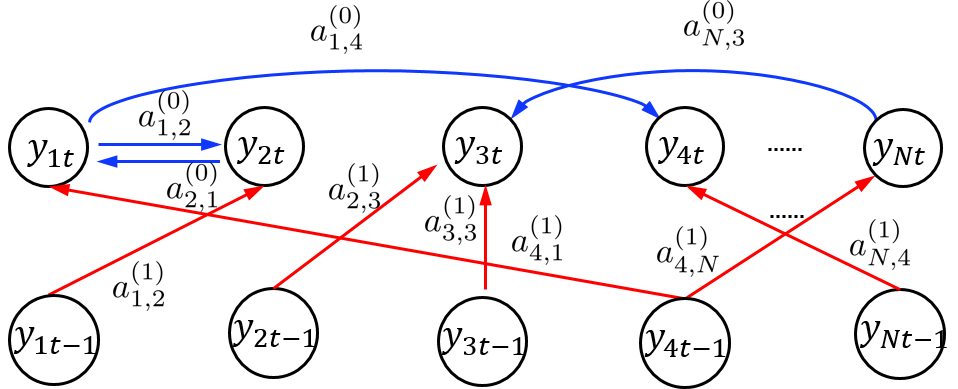
with , and considered known. The SVARM in (4) is a better fit for time-series over graphs compared to the SEM in (2), because it further accounts for temporal dynamics of through the time-lagged influence term . For this reason, SVARMs will be employed for dynamic setups, such as modeling ECoG time series in brain networks, and predicting Internet router delays. The SVARM is depicted in Fig. 1.
II-B Problem statement
Application-specific constraints allow only for a limited number of samples across nodes per slot . Suppose that noisy samples of the -th observation vector
| (5) |
are available, where contains the indices of the sampled vertices, and models the observation error. With , and , the observation model is
| (6) |
where is an matrix with entries , set to one, and the rest set to zero.
The broad goal of this paper is the joint inference of the hidden network topology and signals over graphs (JISG) from partial observations of the latter. Given the observations collected in accordance to the sampling matrices , one aims at finding the underlying topologies, for the SEM, or and for the SVARM, as well as reconstructing the graph process at all nodes . The complexity of the estimators should preferably scale linearly in . As estimating the topology and relies on partial observations, this is a semi-blind inference task.
III Jointly inferring topology and signals
Given in (6), this section develops a novel approach to infer , and . To this end, we advocate the following regularized least-squares (LS) optimization problem
| (7) | ||||
where tunes the relative importance of the fitting term; , control the effect of the -norm and the Frobenius-norm, respectively, and . The weighted sum of and is the so-termed elastic net penalty, which promotes connections between highly correlated nodal measurements. The elastic net targets the “sweet spot” between the regularizer that effects sparsity, and the regularizer, which advocates fully connected networks [37].
Even though (7) is nonconvex in both and due to the bilinear product , it is convex with respect to (w.r.t.) each block variable separately. This motivates an iterative block coordinate descent (BCD) algorithm that alternates between estimating and .
Given , the estimates are found by solving the quadratic problem
| (8) |
where the regularization terms in (7) do not appear. Clearly, (8) conveniently decouples across as
| (9) |
The first quadratic in (9) can be written as , and it can be viewed as a regularizer for , promoting graph signals with similar values at neighboring nodes. Notice that (9) may not be strongly convex, since could be rank deficient. Nonetheless, since is smooth, (9) can be readily solved via gradient descent (GD) iterations
| (10) |
where , and is the stepsize chosen e.g. by the Armijo rule [7]. The computational cost of (10) is dominated by the matrix-vector multiplication of with , which is proportional to , where denotes the number of non-zero entries of . Moreover, the learned is expected to be sparse due to the regularizer in (7), which renders first-order iterations (10) computationally attractive, especially when graphs are large. The GD iterations (10) are run in parallel across until convergence to a minimizer of (9).
On the other hand, with available, is found via
| (11) |
where the LS observation error in (7) has been omitted. Note that (11) is strongly convex, and as such it admits a unique minimizer. Hence, we adopt the alternating methods of multipliers (ADMM), which guarantees convergence to the global minimum in a finite number of iterations; see e.g. [13]. The derivation of the algorithm is omitted due to lack of space; instead the detailed derivation of an ADMM solver for a more general setting will be presented in Sec. IV-A.
The BCD solver for JISG is summarized as Algorithm 1. JISG converges at least to a stationary point of (7), as asserted by the ensuing proposition.
Proposition 1.
Proof.
The basic convergence results of BCD have been established in [36]. First, notice that all the terms in (7) are differentiable over their open domain except the non-differentiable norm, which is however separable. These observations establish, based on [36, Lemma 3.1], that is regular at each coordinatewise minimum point , and therefore every such a point is a stationary point of (7). Moreover, is continuous and convex per variable. Hence, by appealing to [36, Theorem 5.1], the sequence of iterates generated by JISG converges monotonically to a coordinatewise minimum point of , and consequently to a stationary point of (7). ∎
A few remarks are now in order.
Remark 1.
A popular alternative to the elastic net regularizer is the nuclear norm that promotes low rank of the learned adjacency matrix - a well-motivated attribute when the graph is expected to exhibit clustered structure [10].
Remark 2.
Oftentimes, prior information about may be available, e.g. the support of ; nonnegative edge weights ; or, the value of for some . Such prior information can be easily incorporated in (7) by adjusting , and the ADMM solver accordingly.
Remark 3.
Remark 4.
In real-world networks, sets of nodes may depend upon each other via multiple types of relationships, which ordinary networks cannot capture [19]. Consequently, generalizing the traditional single-layer to multilayer networks that organize the nodes into different groups, called layers, is well motivated. Such layer structure can be incorporated in (7) via appropriate regularization; see e.g. [17]. Thus, the JISG estimator can also accommodate multilayer graphs.
IV Jointly infer graphs and processes over time
Real-world networks often involve processes that vary over time, with dynamics not captured by SEMs. This section considers an alternative based on SVARMs that allows for joint inference of dynamic network processes and graphs.
IV-A Batch Solver for JISG over time
Given , this section develops an efficient approach to infer , , and . Clearly, to cope with the undetermined system of equations (4) and (6), one has to exploit the structure in and . This prompts the following regularized LS objective
| (12) | ||||
where is a regularization scalar weighting the fit to the observations, and is the elastic net regularizer for the connectivity matrices. The first sum accounts for the LS fitting error of the SVARM, and the second LS cost accounts for the initial conditions. The third term sums the measurement error over . Finally, the elastic net penalty terms , and favor connections among highly correlated nodes; see also discussion after (7).
The optimization problem in (12) is nonconvex due to the bilinear terms , and ; nevertheless, it is convex w.r.t. each of the variables separately. Next, an efficient algorithm based on BCD is put forth that provably attains a stationary point of (12). With , and available, the following objective yields estimates
| (13) |
where denotes the estimate of given . Different from (8), the time-lagged dependencies couple the objective in (IV-A) across . Upon defining that is assumed invertible, , and , we can express (IV-A) equivalently as
| (14) |
The minimizer of (IV-A) can be attained by
| (15) |
where the square matrix weighting the norm in (15) has block entries , , . The minimizer of (15) admits a closed-form solution as . Unfortunately, this direct approach incurs computational complexity , which does not scale favorably. Scalability in can be aided by distributed solvers, which are possible using consensus-based ADMM iterations; see e.g., [13]. With regards to scalability across time, the following proposition establishes that an iterative algorithm attains with complexity that is linear in .
Since (IV-A) is identical to the deterministic formulation of the Rauch-Tung-Striebel (RTS) smoother for a state-space model with state noise covariance and measurement noise covariance , we deduce that the RTS algorithm, see e.g. [4],[27], applies readily to obtain sequentially the structured per slot component . Summing up, we have established the following result.
Proposition 2.
for do
KF1.
KF2.
KF3.
KF4.
KF5.
end for
for do
KS1.
KS2.
end for
Output.
Algorithm 2 is a forward-backward algorithm: The forward direction is executed by Kalman filtering (steps KF1-KF5); and the backward direction is performed by Kalman smoothing (steps KS1-KS2) [27]. The algorithm smooths the state estimates over the interval . Each step incurs complexity at most , and hence the overall complexity for estimating is , which scales favorably for large . For solving (IV-A), one should initialize the RTS by , and .
To estimate the adjacency matrices given , consider the following problem
| (16) |
The objective in (IV-A) is convex albeit nonsmooth, and hence ADMM can be adopted to obtain and . The ADMM solver is summarized as Algorithm 3, and its derivation is deferred to the Appendix.
The overall procedure for joint inference of signals and graphs over time (JISGoT) is tabulated as Algorithm 4. Convergence of JISGoT is asserted in the following proposition, the proof of which is similar to Proposition 1, and hence is omitted.
Proposition 3.
IV-B Fixed-lag solver for online JISGoT
JISGoT performs fixed-interval smoothing, since the whole batch has to be available to learn . Albeit useful for applications such as processing electroencephalograms, and analysis of historical trade transaction data, this batch solver is not suitable for online applications, such as stock market prediction, analysis of online social networks, and propagation of cascades over interdependent power networks. Such applications enforce strict delay constraints and require estimates within a window or fixed lag [4].
Driven by the aforementioned delay constraints, the goal here is to estimate , relying upon observations up to time , with denoting the affordable delay window length. Supposing that a KF (cf. Algorithm 2) has been run up to time to yield estimates and , the desired estimates can be obtained at by solving the following problem
| (17) | ||||
where and are the solutions to (17) at , and controls the effect of the LS terms that promote slow-varying . Similar to (12), the fixed-lag objective (17) will be solved via a BCD algorithm to a stationary point. Observe that solving (17) for is a special case of the fixed-interval objective in (IV-A), when the initial condition on the state, namely , and , are given by the RTS algorithm, and the state is smoothed over the interval ; see [4] for details on the fixed-lag smoother. Solving for entails the additional quadratic terms relative to (IV-A) that can be easily incorporated in Algorithm 3.
Thus, one can employ Algorithm 4 with minor modifications to solve the fixed-lag objective (17) and estimate . As a convenient byproduct, the novel online estimator (17) tracks dynamic topologies from the time-varying estimates and . This is well-motivated when the process is non-stationary, and the underlying topologies change over time.
Remark 5.
Although this section builds upon the SVARM in (4) that accounts only for a single time-lag, the proposed algorithms can be readily extended to accommodate SVARMs with multiple time-lags, i.e., . By defining the extended vector process , the block matrix , with entries , and zero otherwise, the block matrix , with entries , for and zero otherwise, and the error vector , the general SVARM can be written as , which resembles a single time-lag SVARM in (4).
V Identifiability analysis
This section provides results on the identifiability of the network topology given observations at subsets of nodes under the noise-free SEM. Specifically, in the absence of noise (2) and (6) with , can be written as
| (18a) | ||||
| (18b) | ||||
where with if , and zero otherwise, and with if , and zero if is not sampled at . The matrix collects all the observations.
Definition 1.
The Kruskal rank of an matrix (denoted hereafter as ) is defined as the maximum number such that any combination of columns of constitutes a full rank matrix.
To establish identifiability results, we rely on a couple of assumptions.
as1. Matrix
has at most non-zero entries per row.
as2.
There exists a subset of columns indexed by , such that the
coresponding
sub-matrix
is fully observable, i.e.,
and
, and .
Proof.
Combining (18a) and (18b) leads to
| (19) |
Considering the equations indexed by along with as2, we have , which leads to the matrix form
| (20) |
Letting and denote the -th rows of and respectively, the row-wise version of (20) can be written as
| (21) |
Suppose there exists a vector with nonzero entries, and , such that the following holds
| (22) |
Combining (22) and (21), we arrive at
| (23) |
Since and both have nonzero entries, vector has at most nonzero entries (see Fig. 2). According to as2, it holds that , and thus any columns of are linearly independent; see Definition 1, which implies and henceforth leads to a contradiction. The argument applies for all . ∎
Theorem 1 establishes the sufficient condition for identifying the network structure given full observations for some . As1 effectively reduces the number of unknowns to at most. As2 asserts that the observation matrix is expressive enough to identify uniquely. However, if one does not have control over the sampling process, may not be observable at all nodes per slot . Therefore, the present paper further investigates the identifiability conditions when only partial observations of the network process are available per slot . The results built upon the following assumption.
as3. For any subset of row indices with , there exists a subset of column indices with that forms the matrix with entries that is fully observable; meaning , and , and satisfies .
Proof.
Combining (18a) and (18b) yields
| (24) |
Collecting the equations over leads to the matrix . Considering the -th row of one obtains
| (25) |
where To argue by contradiction, suppose there exists a vector with nonzero entries, and , such that the following holds
| (26) |
Combining (26) with (25) one arrives at
| (27) |
Since and both have nonzero entries, has at most nonzero entries. Without loss of generality assume that contains all the indices of nonzero entries in . Let denote the sub-vector containing all entries of indexed by . Hence, (27) can be rewritten as
| (28) |
where selects the rows of indexed by . According to as3, for any set of row indices we can find a set of column indices such that is fully observable, and thus . As a result, it holds that
| (29) |
Since , any subset of columns of is linearly independent, which implies , and by definition , which leads to a contradiction. The analysis from (25) to (29) holds for all . ∎
VI Numerical tests
The tests in this section evaluate the performance of the proposed joint inference approach in comparison with state-of-the-art graph signal inference and topology identification techniques using synthetic and real data.
The network topology perfomance is measured by the edge identification error rate (EIER), defined as
with the operator denoting the number of nonzero entries of its argument, and () the support of (). For the estimated adjacency an edge is declared present if exceeds a threshold chosen to yield the smallest EIER. The inference performance of JISG is assessed by comparing with the normalized mean-square error
Parameters , and are selected via cross validation. The software used to conduct all experiments is MATLAB. All results represent averages over 10 independent Monte Carlo runs. Unless otherwise stated, is chosen uniformly at random without replacement over for each with constant size over time; that is, .
VI-A Numerical tests on synthetic data
First, a synthetic network of size was generated using the Kronecker product model, that effectively captures properties of real graphs [21]. It relies on the “seed matrix”
that produces the matrix as , where denotes Kronecker product. The entries of were selected as , and the resulting matrix was rendered symmetric by adding its transpose. The graph signals were generated using the graph-bandlimited model , where , , and are the eigenvectors associated with the 10 smallest eigenvalues of the Laplacian matrix . No noise was added to the observations; that is, .
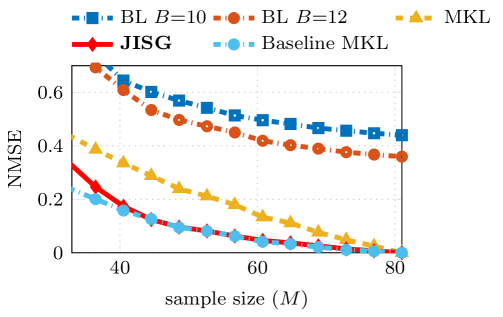
The compared estimators for graph signal inference include the bandlimited estimator (BL) [25, 5] with bandwidth ; and the multi-kernel learning (MKL) estimator that employs a dictionary comprising 100 diffusion kernels with parameter uniformly spaced between 0.01 and 2, and selects the kernel that “fits” best the observed data [29]. These reconstruction algorithms assume the topology is known and symmetric, which may not always be the case. To capture model mismatch, BL and MKL use with instead of . Fig. 4 shows the NMSE of various approaches with increasing , where , and the baseline is the MKL that considers the true topology . The reconstruction performance of JISG is superior compared to that of BL and MKL, and matches the baseline performance. Moreover, the reported CPU time of JISG at 0.12 seconds was an order of magnitude faster than that of the MKL baseline at 1.6 seconds.
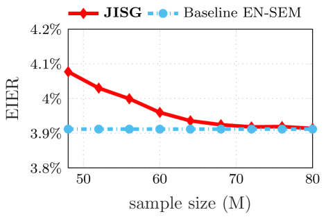
For the same simulation setting, the topology inference performance was evaluated, by comparing with the elastic net (EN) SEM that identifies the network topology from observations across all nodes, meaning . Fig. 5 plots the EIER with increasing for JISG while EN-SEM uses . The semi-blind novel approach achieves similar performance with the baseline, which can not cope with missing nodal measurements.
VI-B Gene regulatory network identification
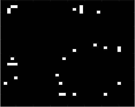
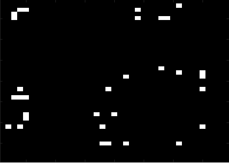
Further tests were conducted using real gene exrpession data [8]. Nodes in this network represent immune-related genes, while the measurements consist of gene expression data from unrelated Nigerian individuals. The graph process measures the expression level of gene for individual . This experiment evaluates the topology inference performance of JISG with genes for all individuals sampled at random. Since no ground-truth topology is available here, the estimated adjacency of EN-SEM, that relies on all the observations, was used for comparison. Fig. 6 depicts heatmaps of the estimated adjacencies. As observed, JISG learns a topology similar to that identified by EN-SEM, and imputes the missing values with NMSE . Therefore, our joint inference approach is capable of revealing causal dependencies even when gene expression data contain missing values.
VI-C Temperature prediction
Consider the National Climatic dataset, which comprises hourly temperature measurements at measuring stations across the continental United States in 2010 [1]. The value represents here the -th temperature sample recorded at the -th station. For evaluating the JISGoT the cumulative NMSE (cNMSE) was used
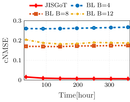
Next, the proposed method is compared to the graph-bandlimited approach [5, 25] for different bandwidth values , where a time-invariant graph was constructed as in [28], based on geographical distances. Fig. 7 reports the cNMSE performance of the estimators with for increasing . JISGoT learns the latent topology among sensors and outperforms the band-limited estimator since the temperature may not adhere to the band-limited model for the geographical graph.
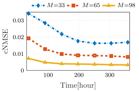
Fig. 8 shows the cNMSE of JISGoT with variable . As expected, the performance improves with increasing number of samples, while with just 30% sampled stations the normalized reconstruction error is only 0.018. Hence, JISGoT can be employed to effectively predict missing sensor measurements.
VI-D GDP prediction
This experiment is carried over the gross domestic product (GDP) dataset [2], which comprises GDP per capita for countries for the years 1960-2016. The process now denotes the GDP reported at the -th country and -th year for . Fig. 9 shows the cNMSE performance of our joint approach for different . The semi-blind estimator unveils the latent connections among countries, while it reconstructs the GDP with cNMSE=0.05 when 60% samples are available.
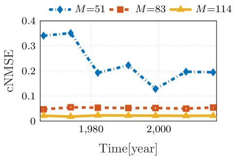
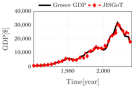
Fig. 10 depicts the true values, along with the GDP estimates of Greece for , which corroborates the effectiveness of JISGoT in predicting the GDP evolution and henceforth facilitating economic policy planning.
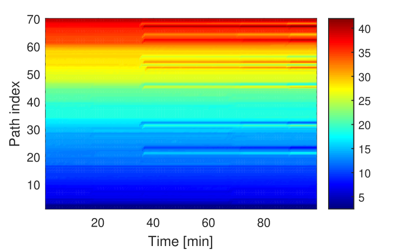
VI-E Network delay prediction
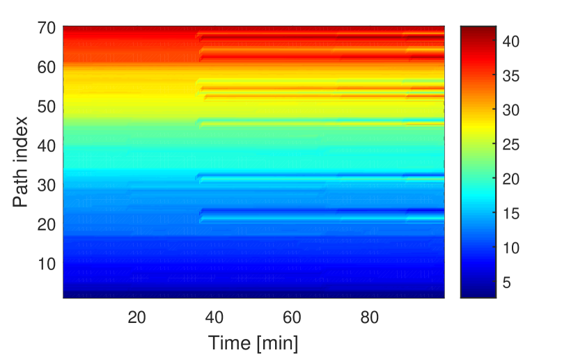
The last dataset records measurements of path delays on the Internet2 backbone[3]. The network comprises 9 end-nodes and directed links. The delays are available for paths per minute. Function denotes the delay in milliseconds measured at the -th path and -th minute.
The proposed JISGoT will be evaluated in estimating the delay over the network from randomly sampled path delays. To that end, delay maps are traditionally employed, which depict the network delay per path over time and enable operators to perform troubleshooting. The paths for the delay maps in Fig. 11 are sorted in increasing order of the true delay at . Clearly, the delay map recovered by JISGoT in Fig. 11(b) visually resembles the true delay map in Fig. 11(a).
VII Conclusions and future work
This paper puts forth a novel framework based on SVARMs and SEMs to jointly infer sparse directed network topologies, and even dynamic graph processes. Efficient minimization approaches are developed with provable convergence that alternate between reconstructing the network processes and inferring the topologies using ADMM. The framework was broadened to facilitate real-time sequential joint-estimation by employing a fixed-lag solver. Recognizing the challenges related to partially observed processes, conditions under which the network can be uniquely identified were derived. Numerical tests on synthetic and real data-sets demonstrate the competitive performance of JISG and JISGoT in both inferring graph signals and the underlying network topologies.
Future research could pursue learning nonlinear models of the network processes, and distributed implementation of JISG, which is well-motivated, especially when dealing with large-scale networks.
-A ADMM solver for (IV-A)
Towards deriving the ADMM solver, consider , , and the auxiliary variables and . Then, re-write (IV-A) as
| (30) |
The augmented Lagrangian of (-A) is
| (31) |
where and denote Lagrange multiplier matrices, while is the penalty parameter. Henceforth, square brackets denote ADMM iteration indices. The ADMM update for results from that gives
| (32) | ||||
where , . Similarly for , taking results to
| (33) |
where . The elementwise soft-thresholding operator is defined as
Accordingly, the update for is
| (34) |
and for it is
| (35) |
Finally, the Lagrange multiplier updates are given by
| (36a) | |||
| (36b) | |||
The complexity of (32) and (-A) is , while for (-A)-(36) is that leads to an overall per ADMM iteration complexity of , governed by the updates for and . That brings the overall complexity of the algorithm to , where is the number of required ADMM iterations until convergence.
References
- [1] “1981-2010 U.S. climate normals,” [Online]. Available: https://www.ncdc.noaa.gov/data-access.
- [2] “GDP per capita (current US),” [Online]. Available: https://data.worldbank.org/indicator/NY.GDP.PCAP.CD.
- [3] “One-way ping internet2,” [Online]. Available: http://software.internet2.edu/owamp/.
- [4] B. D. Anderson and J. B. Moore, Optimal Filtering. Prentice Hall, 1979.
- [5] A. Anis, A. Gadde, and A. Ortega, “Efficient sampling set selection for bandlimited graph signals using graph spectral proxies,” IEEE Trans. Sig. Process., vol. 64, no. 14, pp. 3775–3789, Jul. 2016.
- [6] J. A. Bazerque, B. Baingana, and G. B. Giannakis, “Identifiability of sparse structural equation models for directed and cyclic networks,” in Global Conf. Sig. Inf. Process., Austing, TX, Dec. 2013, pp. 839–842.
- [7] D. Bertsekas, Nonlinear Programming. Athena Scientific Belmont, 1999.
- [8] X. Cai, J. A. Bazerque, and G. B. Giannakis, “Inference of gene regulatory networks with sparse structural equation models exploiting genetic perturbations,” PLoS Comp. Biol., vol. 9, no. 5, p. e1003068, May 2013.
- [9] G. Chen, D. R. Glen, Z. S. Saad, J. P. Hamilton, M. E. Thomason, I. H. Gotlib, and R. W. Cox, “Vector autoregression, structural equation modeling, and their synthesis in neuroimaging data analysis,” Computers in Biology and Medicine, vol. 41, no. 12, pp. 1142–1155, 2011.
- [10] Y. Chen, A. Jalali, S. Sanghavi, and H. Xu, “Clustering partially observed graphs via convex optimization,” J. Mach. Learn. Res., vol. 15, no. 1, pp. 2213–2238, 2014.
- [11] X. Dong, D. Thanou, P. Frossard, and P. Vandergheynst, “Learning Laplacian matrix in smooth graph signal representations,” IEEE Trans. Sig. Process., vol. 64, no. 23, pp. 6160–6173, Dec. 2016.
- [12] G. B. Giannakis, Y. Shen, and G. V. Karanikolas, “Topology identification and learning over graphs: Accounting for nonlinearities and dynamics,” Proc. of the IEEE, vol. 106, no. 5, pp. 787–807, May 2018.
- [13] G. B. Giannakis, Q. Ling, G. Mateos, I. D. Schizas, and H. Zhu, “Decentralized learning for wireless communications and networking,” in Splitting Methods in Communication, Imaging, Science, and Engineering. Springer, 2016, pp. 461–497.
- [14] A. S. Goldberger, “Structural equation methods in the social sciences,” Econometrica, vol. 40, no. 6, pp. 979–1001, Nov. 1972.
- [15] V. N. Ioannidis, A. N. Nikolakopoulos, and G. B. Giannakis, “Semi-parametric graph kernel-based reconstruction,” in Global Conf. Sig. Inf. Process., Montreal, Canada, Nov. 2017.
- [16] V. N. Ioannidis, D. Romero, and G. B. Giannakis, “Learning dynamic processes over dynamic graphs via a multi-kernel kriged Kalman filter,” IEEE Trans. Sig. Process., vol. 66, no. 12, pp. 3228–3239, Jun. 2017.
- [17] V. N. Ioannidis, P. A. Traganitis, Y. Shen, and G. B. Giannakis, “Kernel-based semi-supervised learning over multilayer graphs,” in Proc. IEEE Int. Workshop Sig. Process. Advances Wireless Commun., Kalamata, Greece, Jun. 2018.
- [18] D. Kaplan, Structural Equation Modeling: Foundations and Extensions. Sage, 2009.
- [19] M. Kivelä, A. Arenas, M. Barthelemy, J. P. Gleeson, Y. Moreno, and M. A. Porter, “Multilayer networks,” Journal of Complex Networks, vol. 2, no. 3, pp. 203–271, 2014.
- [20] E. D. Kolaczyk, Statistical Analysis of Network Data: Methods and Models. Springer New York, 2009.
- [21] J. Leskovec, D. Chakrabarti, J. Kleinberg, C. Faloutsos, and Z. Ghahramani, “Kronecker graphs: An approach to modeling networks,” J. Mach. Learn. Res., vol. 11, no. 2, pp. 985–1042, Feb. 2010.
- [22] P. D. Lorenzo, S. Barbarossa, P. Banelli, and S. Sardellitti, “Adaptive least mean-square estimation of graph signals,” IEEE Trans. Sig. Info. Process. Netw., vol. 3, no. 4, pp. 555–568, Dec. 2016.
- [23] A. G. Marques, S. Segarra, G. Leus, and A. Ribeiro, “Stationary graph processes and spectral estimation,” IEEE Trans. Sig. Process., vol. 65, no. 22, pp. 5911–5926, Nov. 2017.
- [24] B. Muthén, “A general structural equation model with dichotomous, ordered categorical, and continuous latent variable indicators,” Psychometrika, vol. 49, no. 1, pp. 115–132, Mar. 1984.
- [25] S. K. Narang, A. Gadde, E. Sanou, and A. Ortega, “Localized iterative methods for interpolation in graph structured data,” in Global Conf. Sig. Inf. Process., Austin, Texas, 2013, pp. 491–494.
- [26] X. Ning and G. Karypis, “Slim: Sparse linear methods for top-n recommender systems,” in Proc. of Intl. Conf. on Data Mining, Vancouver, Canada, Dec. 2011, pp. 497–506.
- [27] H. E. Rauch, C. T. Striebel, and F. Tung, “Maximum likelihood estimates of linear dynamic systems,” American Institute Aeronautics Astronautics J., vol. 3, no. 8, pp. 1445–1450, 1965.
- [28] D. Romero, V. N. Ioannidis, and G. B. Giannakis, “Kernel-based reconstruction of space-time functions on dynamic graphs,” IEEE J. Sel. Topics Sig. Process., vol. 11, no. 6, pp. 1–14, Sep. 2017.
- [29] D. Romero, M. Ma, and G. B. Giannakis, “Kernel-based reconstruction of graph signals,” IEEE Trans. Sig. Process., vol. 65, no. 3, pp. 764–778, Feb. 2017.
- [30] S. Sardellitti, S. Barbarossa, and P. D. Lorenzo, “Graph topology inference based on transform learning,” in Global Conf. Sig. Inf. Process., Dec. 2016, pp. 356–360.
- [31] Y. Shen, B. Baingana, and G. B. Giannakis, “Nonlinear structural vector autoregressive models for inferring effective brain network connectivity,” 2016. [Online]. Available: https://arxiv.org/abs/1610.06551
- [32] ——, “Tensor decompositions for identifying directed graph topologies and tracking dynamic networks,” IEEE Trans. Sig. Process., vol. 65, no. 14, pp. 4004–4018, July 2017.
- [33] ——, “Kernel-based structural equation models for topology identification of directed networks,” IEEE Trans. Sig. Proc., vol. 65, no. 10, pp. 2503–2516, May 2017.
- [34] D. I. Shuman, S. K. Narang, P. Frossard, A. Ortega, and P. Vandergheynst, “The emerging field of signal processing on graphs: Extending high-dimensional data analysis to networks and other irregular domains,” IEEE Sig. Process. Mag., vol. 30, no. 3, pp. 83–98, May 2013.
- [35] A. J. Smola and R. I. Kondor, “Kernels and regularization on graphs,” in Learning Theory and Kernel Machines. Springer, 2003, pp. 144–158.
- [36] P. Tseng, “Convergence of a block coordinate descent method for nondifferentiable minimization,” J. of Opt. Theory and Appl., vol. 109, no. 3, pp. 475–494, 2001.
- [37] H. Zou and T. Hastie, “Regularization and variable selection via the elastic net,” J. of the Royal Stat. Soc.: Series B, vol. 67, no. 2, pp. 301–320, 2005.