A Hierarchical Max-Infinitely Divisible Spatial Model for Extreme Precipitation

Abstract

Understanding the spatial extent of extreme precipitation is necessary for determining flood risk and adequately designing infrastructure (e.g., stormwater pipes) to withstand such hazards. While environmental phenomena typically exhibit weakening spatial dependence at increasingly extreme levels, limiting max-stable process models for block maxima have a rigid dependence structure that does not capture this type of behavior. We propose a flexible Bayesian model from a broader family of (conditionally) max-infinitely divisible processes that allows for weakening spatial dependence at increasingly extreme levels, and due to a hierarchical representation of the likelihood in terms of random effects, our inference approach scales to large datasets. Therefore, our model not only has a flexible dependence structure, but it also allows for fast, fully Bayesian inference, prediction and conditional simulation in high dimensions. The proposed model is constructed using flexible random basis functions that are estimated from the data, allowing for straightforward inspection of the predominant spatial patterns of extremes. In addition, the described process possesses (conditional) max-stability as a special case, making inference on the tail dependence class possible. We apply our model to extreme precipitation in North-Eastern America, and show that the proposed model adequately captures the extremal behavior of the data. Interestingly, we find that the principal modes of spatial variation estimated from our model resemble observed patterns in extreme precipitation events occurring along the coast (e.g., with localized tropical cyclones and convective storms) and mountain range borders. Our model, which can easily be adapted to other types of environmental datasets, is therefore useful to identify extreme weather patterns and regions at risk.

KEY WORDS: max-infinitely divisible process; max-stable process; sub-asymptotic extremes; block maxima.

1 INTRODUCTION

The risk of precipitation-induced flooding (pluvial flooding) is strongly determined by the spatial extent of severe storms, and therefore, there is a need to adequately describe the spatial dependence properties of extreme precipitation. With this goal in mind, we propose a scalable model for spatial extremes that relaxes the rigid dependence structure of asymptotic max-stable models, characterizes the main modes of spatial variability using interpretable spatial factors, and allows for easy prediction at unobserved locations. The areal aspect of extreme precipitation plays a role in flood risk assessment. Precipitation falling over a single drainage basin flows into a common outlet, the aggregate effects of which can be devastating in large volumes. In 2006, heavy precipitation over the Susquehanna River basin in New York and Pennsylvania caused record high discharges along the Susquehanna River and flooding in the region, ultimately leading to federal-level disaster declarations and disaster-recovery assistance from the US Federal Emergency Management Agency (FEMA) in excess of $227 million (Suro et al., 2009).

The last decade has seen a considerable amount of research on the spatial dependence modeling of extremes, in part because of the hazard that extreme weather events pose to human life and property. For recent reviews, see Davison et al. (2012, 2013, 2019) and Davison and Huser (2015). The classical geostatistical Gaussian process models that are ideal for modeling the bulk of a distribution have weak tail-dependence and do not enforce the specific type of positive dependence structure inherent to extremes. Two classes of models, max-stable processes (de Haan and Ferreira, 2006) and generalized Pareto processes (Ferreira and de Haan, 2014; Thibaud and Opitz, 2015), have proven to be useful tools for the modeling of spatial extremes. Max-stable process models are infinite-dimensional generalizations of the limiting models for componentwise maxima. They are asymptotically justified models for pointwise maxima over an infinite collection of independent processes after suitable renormalization, a property which has made them prime candidates for the modeling of spatial extremes. In practice, maxima are taken over large, but finite blocks (e.g., months, years). An approximation error is incurred when applying limiting models to pointwise maxima over finite blocks, and the degree of this error will depend on the rate of convergence of the modeled process as the block size grows. Furthermore, the approximation error is more pronounced when the observed process exhibits weakening spatial dependence at increasingly high quantiles, as the spatial dependence of limiting max-stable processes is the same across all levels of the distribution, and hence would overestimate the level of dependence in the data. For more discussion, see, e.g., Wadsworth and Tawn (2012). Empirical evidence has shown that environmental processes often exhibit weakening spatial dependence at more extreme levels, which has led some to consider non-limiting models for flexible tail dependence modeling (Morris, 2016; Huser et al., 2017, 2018; Huser and Wadsworth, 2019). In particular, Morris (2016) use a random partition of their spatial domain and locally defined, asymptotically dependent skew-t processes to induce long-range asymptotic independence but short-range asymptotic dependence.

In this paper, we aim to extend a class of max-stable models in order to flexibly capture spatial dependence characteristics for sub-asymptotic block maxima data, while still retaining the positive dependence structure inherent to distributions for maxima. The general class of models that we consider, which nests the class of max-stable models, are known as max-infinitely divisible (max-id) processes (Resnick, 1987, Chapter 5). Suppose a random vector $\mathbf{X}$ has joint distribution $F_{X}$, then the distribution of maxima of $n$ independent and identically distributed (i.i.d.) replicates $\mathbf{X}_{1},\ldots,\mathbf{X}_{n}$, taken componentwise, has distribution function $F_{X}^{n}$. The max-id property applies to the converse statement. Suppose that $\mathbf{Z}$ is a random vector of componentwise maxima, composed from a collection of $n$ i.i.d. vectors. Then if $\mathbf{Z}$ has distribution function $G$, there exists some root distribution $F$ such that $G(\mathbf{z})=F^{n}(\mathbf{z})$, or equivalently such that $G^{1/n}(\mathbf{z})=F(\mathbf{z})$. By continuous extension of the relation $G^{q/r}=F$ for $q,r\in\mathbb{N}$, we say that a distribution $G$ is max-id if and only if $G^{s}$ is a valid distribution for all real $s>0$. This is always the case for univariate distributions, but may not necessarily be so for multivariate distributions. Informally, max-id distributions are those which arise from taking componentwise maxima of i.i.d. random vectors and are therefore an appropriate class to constrain ourselves to if the goal is to model componentwise maxima. By slight abuse of language, we say that a spatial process is max-id if all its finite-dimensional distributions are max-id. Necessary and sufficient conditions for max-infinitely divisibility of a distribution function in $\mathbb{R}^{2}$ were first given by Balkema and Resnick (1977). More recently, mixing conditions for stationary max-id processes were explored by Kabluchko and Schlather (2010), and minimality of their spectral representations were described in Kabluchko and Stoev (2016).

Unlike limiting max-stable process models, which have a rigid spatial dependence structure, sub-families of the broader class of max-id processes do not impose such constraints and can accommodate different spatial dependence characteristics across various levels of a distribution see, e.g. Padoan, 2013, Huser et al., 2018. It is the lack of this feature that can cause max-stable processes to fit poorly, as many processes of interest may exhibit spatial dependence at extreme but finite levels. Extrapolation of max-stable fits to higher quantiles in this scenario can cause overestimation of the risk of concurrent extremes (Davison et al., 2013). Furthermore, the challenge of performing conditional simulation from max-stable models given observed values at many locations is a limiting factor for their use in practice (Dombry et al., 2013). The Bayesian model that we develop in the remainder of the paper permits a conditional, hierarchical representation in terms of random effects that facilitates fast conditional simulation, which is useful for prediction at unobserved locations, and for handling missing values.

2 HIERARCHICAL CONSTRUCTION OF SPATIAL MAX-ID MODELS

2.1 Max-Stable Reich and Shaby (2012) Model

Our proposed approach is an extension of the Bayesian hierarchical model developed by Reich and Shaby (2012), which we review here. The Reich and Shaby (2012) model possesses the max-stability property while being tractable in high-dimensions due to its conditional representation in terms of positive-stable variables see also Fougères et al., 2009 and Stephenson, 2009. Let $\alpha\in(0,1)$ and consider a set of independent $\alpha$-stable random variables $A_{1},\ldots,A_{L}{\ {\buildrel\rm{iid}\over{\sim}}\ }{\rm PS}(\alpha)$, where generically the Laplace transform of $A\sim{\rm PS}(\alpha)$ has the form: ${\rm E}\{\exp(-sA)\}=\exp(-s^{\alpha}),\,s\geq 0$. Then we construct the spatial process $Z({\bm{s}})$ as the product of two independent processes,

$$Z({\bm{s}})=\varepsilon({\bm{s}})Y({\bm{s}}),$$ (1)

where $\varepsilon({\bm{s}})$ is a white noise process (i.e., an everywhere-independent multiplicative nugget effect) with $(1/\alpha)$-Fréchet marginals, ${\rm Pr}\{\varepsilon({\bm{s}})\leq z\}=\exp(-z^{-1/\alpha})$, and $Y({\bm{s}})$ is a spatially dependent process defined as an $L^{p}$-norm (for $p=1/\alpha$) of scaled, spatially-varying basis functions $K_{l}({\bm{s}})\geq 0$, $l=1,\ldots,L$:

$$Y({\bm{s}})=\left\{\sum_{l=1}^{L}A_{l}K_{l}({\bm{s}})^{1/\alpha}\right\}^{\alpha}.$$ (2)

The white noise process $\varepsilon({\bm{s}})$ functions as a nugget effect, and accounts for measurement error occurring independently of the underlying process of interest. For small $\alpha$, the contribution of $Y({\bm{s}})$ dominates that of the nugget effect, and vice-versa for large $\alpha$.

Reich and Shaby (2012) used fixed, deterministic spatial basis functions. In other words, they assumed a Dirac prior on the space of valid basis functions, based on the following construction: let $\bm{v}_{1},\ldots,\bm{v}_{L}\in{\mathcal{S}}\in\Real^{p}$ be a collection of spatial knots over our spatial domain of interest ${\mathcal{S}}$, and $K_{l}({\bm{s}})$, $l=1,\ldots,L$, be Gaussian densities centered at each knot $\bm{v}_{l}$, normalized such that $\sum_{l=1}^{L}K_{l}({\bm{s}})=1$ for all ${\bm{s}}\in{\mathcal{S}}$. The Gaussian density basis functions may be replaced with normalized functions from a much broader class while still giving a valid construction for $Y({\bm{s}})$ in (2). A more flexible prior for the kernels $K_{l}({\bm{s}})$, $l=1,\ldots,L$, is discussed in Section 2.3.

The process $\{Z({\bm{s}}),{\bm{s}}\in\mathcal{S}\}$ has finite-dimensional distributions

$${\rm Pr}\{Z({\bm{s}}_{1})\leq z_{1},\ldots,Z({\bm{s}}_{D})\leq z_{D}\}=\exp\left(-\sum_{l=1}^{L}\left[\sum_{j=1}^{D}\left\{z_{j}/K_{l}({\bm{s}}_{j})\right\}^{-1/\alpha}\right]^{\alpha}\right),\quad z_{1},\ldots,z_{D}>0$$ (3)

see Tawn, 1990, which follows from the Laplace transform of an $\alpha$-stable variable. From (3) and the sum-to-one constraint, the marginal distributions are unit Fréchet, i.e., for all ${\bm{s}}\in{\mathcal{S}}$,

$${\rm Pr}\{Z({\bm{s}})\leq z\}=\exp\left(-\sum_{l=1}^{L}\left[\left\{z/K_{l}({\bm{s}})\right\}^{-1/\alpha}\right]^{\alpha}\right)=\exp\left\{-z^{-1}\sum_{l=1}^{L}K_{l}({\bm{s}})\right\}=\exp\left(-z^{-1}\right),\quad z>0.$$

Max-stability follows from (3) by checking that

$${\rm Pr}\{Z({\bm{s}}_{1})\leq nz_{1},\ldots,Z({\bm{s}}_{D})\leq nz_{D}\}^{n} ={\rm Pr}\{Z({\bm{s}}_{1})\leq z_{1},\ldots,Z({\bm{s}}_{D})\leq z_{D}\}.$$ (4)

The max-stability property of $Z({\bm{s}})$ makes it suitable for modeling spatial extremes in scenarios of strong, non-vanishing upper tail dependence. In Section 2.2, we propose a more general max-id model, which can better cope with weakening tail dependence.

Inference may be efficiently performed by taking advantage of the inherent hierarchical structure of the Reich and Shaby (2012) model, noticing that the data are independent conditional on the latent variables $\{A_{l}\}_{l=1}^{L}$, and may be written in terms of the Fréchet distribution with scale parameter $Y({\bm{s}})>0$ and shape parameter $1/\alpha>0$:

$$Z({\bm{s}})|A_{1},\ldots,A_{L}\overset{indep}{\sim}\text{Fr\'{e}chet}(Y({\bm{s}}),1/\alpha),\\$$ (5)

for all ${\bm{s}}\in\mathcal{S}$; that is, ${\rm Pr}\{Z({\bm{s}})\leq z\mid A_{1},\ldots,A_{L}\}=\exp[-\{z/Y({\bm{s}})\}^{-1/\alpha}]$, $z>0$.

2.2 Sub-Asymptotic Modeling Based on a Max-Infinitely Divisible Process

Despite the appealing properties of the Reich and Shaby (2012) model, its deterministic basis functions and its max-stability make it fairly rigid in practice. Max-id processes are natural, flexible, sub-asymptotic models, that extend the class of max-stable processes while still possessing desirable properties reflecting the specific positive dependence structure of maxima. From (4), we can see that max-stable processes are always max-id. Therefore, the former form a smaller subclass within the latter.

The tail dependence class strongly determines how the probability of joint exceedances of a high threshold extrapolates to extreme quantiles. A random vector $(X_{1},X_{2})^{\top}$ with marginal distributions $F_{1}$ and $F_{2}$ is said to be asymptotically independent if ${\rm Pr}\{F_{1}(X_{1})>u\mid F_{2}(X_{2})>u\}\to 0$ as $u\rightarrow 1$, and asymptotically dependent otherwise (Coles et al., 1999). We say that a spatial process {$X({\bm{s}}),{\bm{s}}\in\mathcal{S}\}$ is asymptotically independent if $X({\bm{s}}_{1})$ and $X({\bm{s}}_{2})$ are asymptotically independent for all ${\bm{s}}_{1},{\bm{s}}_{2}\in\mathcal{S}$, ${\bm{s}}_{1}\neq{\bm{s}}_{2}$. Max-stable processes are always asymptotically dependent (except in the case of complete independence) and, therefore, they lack flexibility to adequately capture the tail behavior of asymptotically independent data. In this section, we propose an asymptotically independent max-id model that possesses the max-stable Reich and Shaby (2012) model on the boundary of its parameter space. Dependence properties are further detailed in Section 2.5.

To extend the Reich and Shaby (2012) model to a more flexible max-id formulation, we can change the distribution of the underlying random basis coefficients $\{A_{l}\}_{l=1}^{L}$. The heavy-tailedness of the ${\rm PS}(\alpha)$ distribution yields asymptotic dependence and, by construction, max-stability. To achieve asymptotic independence while staying within the class of max-id processes, we can consider a lighter-tailed, exponentially tilted, positive-stable distribution,

$$A_{1},\ldots,A_{L}{\ {\buildrel\rm{iid}\over{\sim}}\ }{\rm H}(\alpha,\delta,\theta),\qquad\alpha\in(0,1),\delta>0,\theta\geq 0,$$ (6)

which was first introduced by Hougaard (1986) and further studied by Crowder (1989), and has Laplace transform

$${\rm E}\left\{\exp\left(-sX\right)\right\} =\exp\left[-{\delta\over\alpha}\left\{(\theta+s)^{\alpha}-\theta^{\alpha}\right\}\right],\qquad X\sim{\rm H}(\alpha,\delta,\theta).$$ (7)

Denote the ${\rm PS}(\alpha)$ density by $f_{{\rm PS}}(x)$. The ${\rm H}(\alpha,\delta,\theta)$ density $f_{\rm H}$ may be expressed in terms of the positive-stable density $f_{{\rm PS}}$ as

$$f_{{\rm H}}(x)={f_{{\rm PS}}\{x(\alpha/\delta)^{1/\alpha}\}({\alpha/\delta})^{1/\alpha}\exp(-\theta x)\over\exp(\delta\theta^{\alpha}/\alpha)},\qquad x>0,$$ (8)

for $\alpha\in(0,1)$, $\theta\geq 0$, and $\delta>0$ (Hougaard, 1986). An efficient algorithm for simulating from ${\rm H}(\alpha,\delta,\theta)$ is given by Devroye (2009). A simple rejection sampler for the case when $\theta$ is not large is given in the Supplementary Material. When $\delta=\alpha$ and $\theta=0$, we recover the positive-stable distribution ${\rm PS}(\alpha)\equiv{\rm H}(\alpha,\alpha,0)$. The parameter $\alpha$ controls the tail decay, with smaller values of $\alpha$ corresponding to heavier-tailed distributions. Moreover, the density becomes increasingly concentrated around one as $\alpha\to 1$. When $\theta>0$, the gamma distribution with shape $\delta$ and rate $\theta$ is obtained as $\alpha\to 0$.

Upon reparameterization in terms of $\alpha^{\star}=\alpha$, $\delta^{\star}=(\delta/\alpha)^{1/\alpha}$ and $\theta^{\star}=(\delta/\alpha)^{1/\alpha}\theta$, we see from (8) that $\delta^{\star}=(\delta/\alpha)^{1/\alpha}$ is a scale parameter, which does not affect the dependence structure of our new model. Therefore, in the remainder of this paper, we set $\delta=\alpha$ (i.e., $\delta^{\star}=1$) and use ${\rm H}(\alpha,\alpha,\theta)$ throughout without any loss in flexibility.

When $\delta=\alpha$ and $\theta>0$, $f_{\rm H}$ is an exponentially tilted form of $f_{{\rm PS}}$, where the parameter $\theta$ has the effect of exponentially tapering the tail of $f_{{\rm PS}}$ at rate $\theta$. Other extensions of the positive-stable distribution may also be interesting avenues for future research (e.g., polynomial tilting (Devroye, 2009)). However, our choice of (6) preserves the simplicity of the model while introducing a single parameter, the exponential tilting parameter $\theta$, that is directly connected to the dependence properties of the resulting $Z({\bm{s}})$ process, while allowing for inference that is computationally tractable.

Proposition 2.1.

Let $\{Z({\bm{s}}),{\bm{s}}\in\mathcal{S}\}$ be defined as in (1) with $A_{1},\ldots,A_{L}{\ {\buildrel\rm{iid}\over{\sim}}\ }{\rm H}(\alpha,\alpha,\theta)$, $\alpha\in(0,1)$, $\theta\geq 0$. Then, $Z({\bm{s}})$ is max-id.

Proof.

From (7), the finite-dimensional distributions for $\{Z({\bm{s}}),{\bm{s}}\in\mathcal{S}\}$ based on (6) are

$${\rm Pr}\{ Z({\bm{s}}_{1})\leq z_{1},\ldots,Z({\bm{s}}_{D})\leq z_{D}\}={\rm Pr}\{\varepsilon({\bm{s}}_{1})Y({\bm{s}}_{1})\leq z_{1},\ldots,\varepsilon({\bm{s}}_{D})Y({\bm{s}}_{D})\leq z_{D}\}$$

$$={\rm E}\left({\rm Pr}\left[\varepsilon({\bm{s}}_{1})\leq z_{1}\left\{\sum_{l=1}^{L}A_{l}K_{l}({\bm{s}}_{1})^{1/\alpha}\right\}^{-\alpha},\ldots,\varepsilon({\bm{s}}_{D})\leq z_{D}\left\{\sum_{l=1}^{L}A_{l}K_{l}({\bm{s}}_{D})^{1/\alpha}\right\}^{-\alpha}\mid A_{1},\ldots,A_{L}\right]\right)$$

$$={\rm E}\left(\exp\left[-\sum_{j=1}^{D}z_{j}^{-1/\alpha}\sum_{l=1}^{L}A_{l}K_{l}({\bm{s}}_{j})^{1/\alpha}\right]\right)$$

$$=\prod_{l=1}^{L}{\rm E}\left(\exp\left[-A_{l}\sum_{j=1}^{D}\left\{z_{j}/K_{l}({\bm{s}}_{j})\right\}^{-1/\alpha}\right]\right)$$

$$=\exp\left(L\theta^{\alpha}-\sum_{l=1}^{L}\left[\theta+\sum_{j=1}^{D}\left\{z_{j}/K_{l}({\bm{s}}_{j})\right\}^{-1/\alpha}\right]^{\alpha}\right).$$ (9)

As

$${\rm Pr}\{Z({\bm{s}}_{1})\leq z_{1},\ldots,Z({\bm{s}}_{D})\leq z_{D}\}^{1/n}=\exp\left\{L\left({\theta\over n^{1/\alpha}}\right)^{\alpha}-\sum_{l=1}^{L}\left[\left({\theta\over n^{1/\alpha}}\right)+\sum_{j=1}^{D}\left\{nz_{j}/K_{l}({\bm{s}}_{j})\right\}^{-1/\alpha}\right]^{\alpha}\right\},$$

the finite-dimensional distributions, denoted $G(z_{1},\ldots,z_{D};\alpha,\theta)$, from this new process satisfy
$G(z_{1},\ldots,z_{D};\alpha,\theta)^{1/n}=G(nz_{1},\ldots,nz_{D};\alpha,\theta/n^{1/\alpha})$ for all $n\in\Natural$, and thus the process is max-id. This also confirms that the process is max-stable if and only if $\theta=0$. ∎

In Section 2.3, we specify spatial priors for the basis functions, so Proposition 2.1 should be interpreted conditional on the basis functions.

Marginal distributions are no longer unit Fréchet when $\theta>0$; they may be expressed as

$$G_{{\bm{s}}}(z)={\rm Pr}\{Z({\bm{s}})\leq z\}=\exp\left(L\theta^{\alpha}-\sum_{l=1}^{L}\left[\theta+\left\{z/K_{l}({\bm{s}})\right\}^{-1/\alpha}\right]^{\alpha}\right),\quad z>0.$$ (10)

Bayesian and likelihood-based inference may be performed similarly as before, so this process enjoys the same computational benefits as the Reich and Shaby (2012) model, while having the traditional max-stable Reich and Shaby (2012) process as a special case on the boundary of the parameter space (i.e., when $\theta=0$). Note that unlike the Reich and Shaby (2012) model, here the marginal distributions depend on the dependence parameters $\alpha$ and $\theta$, however, this is not a problem for inference as we adopt a copula-based approach, in which we separate the treatment of the marginal distributions and the dependence structure. Marginal modeling is described in greater detail in Section 2.4. Finally, a spectral representation for the proposed max-id model is described in the Supplementary Material, which makes a link with the max-id models of Huser et al. (2018).

2.3 Prior Specification for the Spatial Kernels Based on Flexible Log-Gaussian Process Factors

The basis functions used in Reich and Shaby (2012), constructed from Gaussian densities, are radial functions, decaying symmetrically from their knot centers. While it is possible to approximate a wide range of extremal functions by considering a large collection of Gaussian density basis functions $K_{1}({\bm{s}}),\ldots,K_{L}({\bm{s}})$ as in (2), the resulting process is overly smooth and artificially non-stationary for fixed $L$. In this section, we propose an alternative prior for the basis functions, which allows for a parsimonious, yet flexible, stationary representation that can give insights into the predominant modes of spatial variability among of the underlying process.

More precisely, we extend the Reich and Shaby (2012) model by replacing the Dirac prior on the Gaussian density basis functions with flexible log-Gaussian process priors, which more closely approximate the features of natural phenomena than radial basis functions. This choice of basis functions is analogous to the construction of the Brown-Resnick process (Brown and Resnick, 1977; Kabluchko et al., 2009), which itself can be represented as the pointwise maximum over an infinite collection of scaled log-Gaussian processes. Let $\tilde{K}_{l}({\bm{s}})$, $l=1,\ldots,L-1$, be i.i.d. mean-zero stationary Gaussian processes, each with exponential covariance function, $C(h)=\delta^{2}\exp(-h/\rho),\,h\geq 0$, whose variance and range are $\delta_{K}^{2}>0$ and $\rho_{K}>0$, respectively. We take the $L$th basis to be the constant function equal to the mean of the Gaussian process, i.e., $\tilde{K}_{L}({\bm{s}})=0$ for all ${\bm{s}}\in{\mathcal{S}}$. Fixing the $L$th term ensures that it is possible to recover the $\tilde{K}_{l}$ from the $K_{l}({\bm{s}})$ terms, which is necessary for making posterior draws of $\tilde{K}_{l}({\bm{s}})$ (see Supplementary Material). Other prior choices for the basis functions that may also be worth exploring include using a more general Matérn class of covariance functions or Gaussian processes with stationary increments and an unbounded variogram (i.e., fractional Brownian motions), akin to the Brown-Resnick process. Application of a fractional Brownian motion prior in this context would require a choice of origin for each basis function, which would increase the computational cost if one wanted to marginalize over that unknown origin, and so we do not pursue it here. To satisfy the sum-to-one constraint for each spatial location ${\bm{s}}\in{\mathcal{S}}$, we set

$$K_{l}({\bm{s}})=\exp\left\{\tilde{K}_{l}({\bm{s}})\right\}/\sum_{l=1}^{L}\exp\left\{\tilde{K}_{l}({\bm{s}})\right\},\quad l=1,\ldots,L.$$ (11)

The variance parameter $\delta_{K}^{2}$ controls the long-range spatial dependence of the max-id process $Z({\bm{s}})$, with smaller values corresponding to stronger long-range dependence (see Davison et al. (2012) for a similar discussion of geometric Gaussian processes). When $\delta_{K}^{2}$ is large, the difference in relative magnitudes of the unnormalized log-Gaussian processes at any given location ${\bm{s}}$ is likely to be larger than when $\delta_{K}^{2}$ is small. Normalizing the basis functions when the difference in magnitudes is great gives way to more volatile fluctuations between dominating basis functions, and hence less long-range dependence. The Gaussian process range parameter $\rho_{K}$ governs the short-range dependence, now with larger values corresponding to stronger short-range dependence. Because the proposed basis functions provide greater flexibility in adapting to the data than the fixed Gaussian density basis, fewer basis functions are needed. In the data application presented in Section 3, we choose the number of basis functions using an out-of-sample log-score criterion. Increasing the number of basis functions allows for greater flexibility in capturing spatially dependent subregions that tend to have extreme events together at the cost of greater computational burden.

When the deterministic basis functions used by Reich and Shaby (2012) are replaced with random ones, the max-stability (when $\theta=0$) and max-infinite divisibility properties should be interpreted conditionally on the basis functions. Both the conditional and unconditional dependence properties are described in Section 2.5.

2.4 Marginal Modeling and Realizations

For marginal distribution modeling, we use the Generalized Extreme-Value (GEV) distribution, which is the asymptotic distribution for univariate block maxima. The ${\rm GEV}(\mu,\sigma,\xi)$ distribution function has the following form:

$$G(z)=\begin{cases}\exp\left[-\exp\left\{-(z-\mu)/\sigma\right\}\right],&\xi=0,\\ \exp[-\{1+\xi(z-\mu)/\sigma\}_{+}^{-1/\xi}],&\xi\neq 0,\end{cases}$$

where $a_{+}=\max(0,a)$, for some location $\mu\in\mathbb{R}$, scale $\sigma>0$, and shape $\xi\in\mathbb{R}$ parameters, with support $\{z\in\mathbb{R}:1+\xi(z-\mu)/\sigma)>0\}$ when $\xi\neq 0$, and $\mathbb{R}$ when $\xi=0$. Since monotone increasing transformations of the marginal distributions do not change the max-id or max-stable dependence structure, we allow for general GEV marginal distributions that are possibly different for each spatial location. In other words, we set $\tilde{Z}({\bm{s}})=\mathrm{GEV}^{-1}[G_{{\bm{s}}}\{Z({\bm{s}})\};\mu({\bm{s}}),\sigma({\bm{s}}),\xi({\bm{s}})]$, where $G_{\bm{s}}(z)$ is the marginal distribution of $Z({\bm{s}})$, which in the case of the Reich and Shaby (2012) model is $G_{\bm{s}}(z)=\exp\left(-z^{-1}\right),z>0$, and in the $\theta>0$ case is given in (10), and $\mathrm{GEV}^{-1}\{\cdot;\mu({\bm{s}}),\sigma({\bm{s}}),\xi({\bm{s}})\}$ is the quantile function for a GEV distribution with location $\mu({\bm{s}})$, scale $\sigma({\bm{s}})>0$, and shape $\xi({\bm{s}})$. We treat $\tilde{Z}({\bm{s}})$ as our response. In subsequent sections, Gaussian process priors are assumed for the GEV parameters $\mu({\bm{s}})$, $\gamma({\bm{s}})=\log\left\{\sigma({\bm{s}})\right\}$, and $\xi({\bm{s}})$, and Markov chain Monte Carlo (MCMC) methods are used to draw posterior samples for this model. The details of the MCMC sampler are given in the Supplementary Material.

To visualize some of the features of our model, we present some sample paths in Figure 1. Realizations of $\tilde{Z}({\bm{s}})$ on the unit square constructed using the Gaussian density ($L=25$ evenly spaced basis functions, with standard deviation $\tau=1/6$) and log-Gaussian process ($L=15$ basis functions, with variance $\delta_{K}^{2}=25$ and range $\rho_{K}=3/4$) basis functions are shown in Figure 1. For illustration, the realizations have standard Gumbel margins everywhere in space, i.e., $\mu({\bm{s}})=\xi({\bm{s}})=0$ and $\sigma({\bm{s}})=1$ for all ${\bm{s}}\in\mathcal{S}$. The figure illustrates the role of $\alpha$ in controlling the relative contribution of the nugget process, and the impact of $\theta$ on the asymptotic dependence structure. Weaker tail dependence is present in the max-id models ($\theta>0$) than their max-stable counterparts ($\theta=0$). Moreover, the general shapes of the Gaussian density basis model realizations appear less resemblant of natural processes than do those from the log-Gaussian process basis model.

While we have only developed the model for a single realization of the process $\tilde{Z}({\bm{s}})$ so far, the model can easily be generalized to accommodate multiple replicates in time, which we will use in Section 3. In particular, treating time replicates of the process to be independent, we denote the maxima process observed at spatial location ${\bm{s}}$ and time $t$ by $\tilde{Z}_{t}({\bm{s}})$, $t=1,\ldots,T$. We assume the marginal GEV parameters and basis functions do not vary in time, but allow the relative contribution of each basis function to be different for different time replicates of the process by taking the random basis coefficients to be $A_{l,t}{\ {\buildrel\rm{iid}\over{\sim}}\ }{\rm H}(\alpha,\alpha,\theta)$, $l=1,\ldots,L$, and $t=1,\ldots,T$.

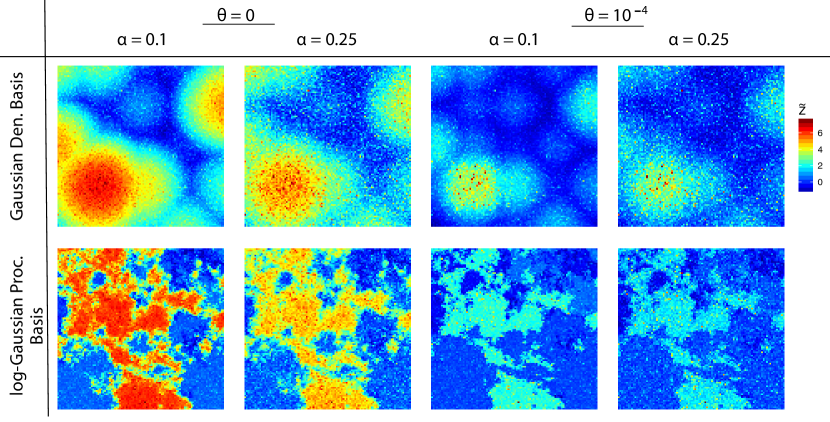
Figure 1: Realizations of the max-stable ($\theta=0$) and max-id ($\theta>0$) processes with Gaussian density (top) and log-Gaussian process (bottom) basis functions, plotted on Gumbel margins.

2.5 Dependence Properties

In this section, we explore the dependence properties of the proposed max-id model. The parameter $\theta$ plays a crucial role in determining the asymptotic dependence class. Reich and Shaby (2012) show that $\{Z({\bm{s}}),{\bm{s}}\in\mathcal{S}\}$ is asymptotically dependent and max-stable for $\alpha\in(0,1)$, $\theta=0$. However, when $\theta>0$, this is no longer the case.

Proposition 2.2.

The process $\{Z({\bm{s}}),{\bm{s}}\in\mathcal{S}\}$ defined in Sections 2.2–2.3 using the log-Gaussian process basis prior in (11) is an asymptotically independent process when $\theta>0$ and asymptotically dependent when $\theta=0$ and $\alpha<1$.

For a proof, see Appendix A. Figure 2 displays two common dependence measures, $\chi_{u}={\rm Pr}\left[G_{{\bm{s}}_{1}}\{Z({\bm{s}}_{1})\}>u\mid G_{{\bm{s}}_{2}}\{Z({\bm{s}}_{2})\}>u\right]$ and $\bar{\chi}_{u}={2\log{\rm Pr}\left[G_{{\bm{s}}_{2}}\{Z({\bm{s}}_{2})\}>u\right]\over\log{\rm Pr}\left[G_{{\bm{s}}_{1}}\{Z({\bm{s}}_{1})\}>u,G_{{\bm{s}}_{2}}\{Z({\bm{s}}_{2})\}>u\right]}$, $0<u<1$ (Coles et al., 1999) to illustrate the role of $\alpha$ and $\theta$ in controlling the dependence properties of the tail process. Although notationally we have omitted the dependence of $\chi_{u}$ on ${\bm{s}}_{1}$ and ${\bm{s}}_{2}$, $\chi_{u}$ will also depend on the locations in the (non-stationary) Gaussian density basis case. Nevertheless, while the Reich and Shaby (2012) max-stable process is non-stationary, it is approximately stationary for a dense set of spatial knots. An attractive feature of the proposed model is that as $\theta\downarrow 0$, $\chi_{u}$ and $\bar{\chi}_{u}$ transition smoothly from weak dependence to strong dependence for all $u<1$.

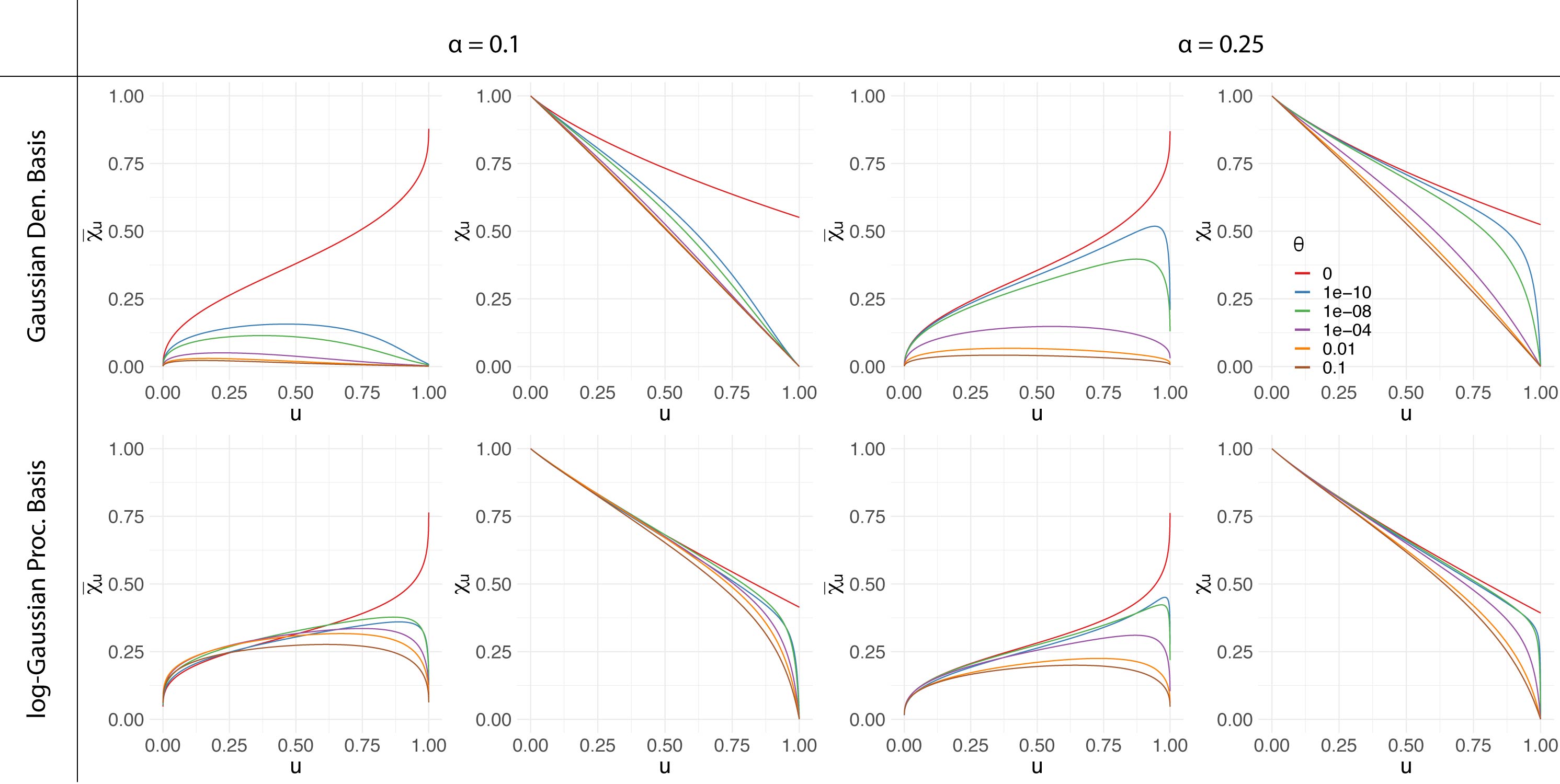
Figure 2: Dependence measures $\bar{\chi}_{u}$ and $\chi_{u}$ for the max-stable ($\theta=0$) and max-id ($\theta>0$) models for $Z(s),s\in\mathbb{R}$, using $L=25$ Gaussian density ($\tau=1/6$) and $L=15$ log-Gaussian process ($\delta^{2}_{K}=25$, $\rho_{K}=3/4$) basis functions for $s_{1}=0$ and $s_{2}=1/4$. The knots of the Gaussian density basis functions are evenly spaced between $0$ and $1$. The figures in the bottom row correspond to $\chi_{u}$ after marginalizing over the log-Gaussian process basis functions based on $M=1,000$ Monte Carlo draws.

The extremal coefficient $\theta_{\mathcal{D}}$, studied by Schlather and Tawn (2003), is a measure of spatial dependence along the diagonal of the finite-dimensional distributions of max-stable processes. It takes on values from $\theta_{\mathcal{D}}=1$ when the components are perfectly dependent to $\theta_{\mathcal{D}}=D$ when they are independent, and therefore can be interpreted as the effective number of independent variables. The finite-dimensional distributions of a max-stable process with unit-Fréchet margins at level $z$ can be written in the form

$$\Pr\left\{Z({\bm{s}}_{1})\leq z,\ldots,Z({\bm{s}}_{D})\leq z\right\}=\exp\left\{-{\theta_{\mathcal{D}}({\bm{s}}_{1},\ldots,{\bm{s}}_{D})\over z}\right\},\quad\theta_{\cal{D}}({\bm{s}}_{1},\ldots,{\bm{s}}_{D})\in[1,D],$$ (12)

where $\theta_{\cal{D}}$ determines the spatial dependence and does not depend on the level $z$. The rigidity of the dependence structure across all quantiles limits the applicability of max-stable models to processes that exhibit varying spatial dependence types at different quantiles. From (9), we can see that the max-id extension of the Reich and Shaby (2012) model does not possess this property for $\theta>0$.

Figure 3 contrasts the spatial dependence features of the proposed models. We examine how the conditional probability of jointly exceeding a fixed quantile decays with increasing distance. Each panel shows the spatial decay of $\chi_{u}$ as a function of increasing spatial lag $h$ for several quantiles. We see qualitatively different behavior in the spatial decay of dependence at different quantiles between the max-stable and max-id models. In the max-stable cases, the conditional exceedance probability $\chi_{u}$ at short spatial lags $h$ is very similar at all levels $u$ of the distribution. The max-id models allow for more flexibility, as can be seen by the attenuated curves for higher quantiles and wider array of spatial decay types. From Figure 3, it can be seen that for $\theta>0$, the parameter $\alpha$ plays a role in how precipitous the decay in spatial dependence is with increasing distance, with smaller $\alpha$ corresponding to steeper decay. Also, just as in Reich and Shaby (2012), $\alpha$ determines the contribution of the nugget effect, which is greater when $\alpha$ is large and lesser when $\alpha$ is small.

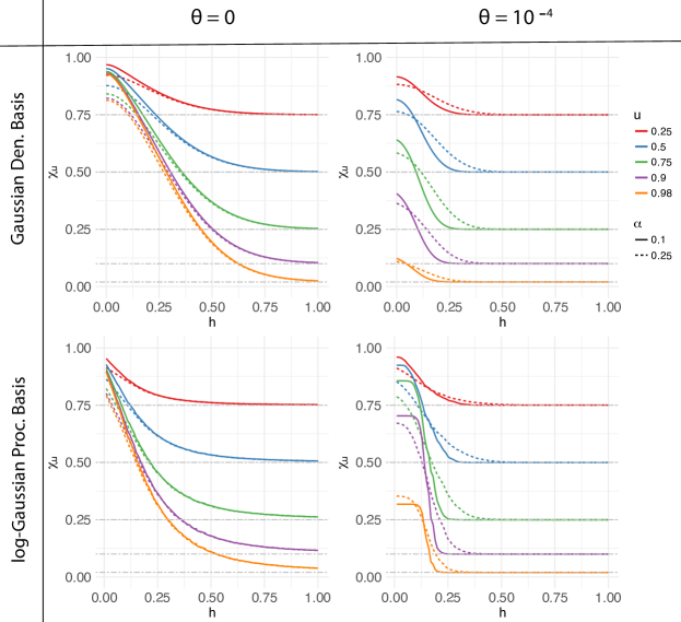
Figure 3: Dependence measure $\chi_{u}(h)$ between $Z(s_{0})$ and $Z(s_{0}+h)$ for $s_{0}=0$ as a function of $h$ for max-stable (left column) and max-id (right column) models on ${\mathcal{S}}=[0,1]$, with $L=25$ Gaussian density basis functions with $\tau=1/6$ (top row) and $L=15$ log-Gaussian process basis functions with $\delta_{K}^{2}=25$ and $\rho_{K}=3/4$ (bottom row) basis functions for varying $\alpha$ and $u$. Gaussian density basis functions are evenly spaced between 0 and 1. Estimates of $\chi_{u}(h)$ in the log-Gaussian process basis model are based on 50,000 Monte Carlo replicates. Horizontal dash-dot gray lines representing the values of $\chi_{u}$ for independent $Z(s_{0})$ and $Z(s_{0}+h)$ are plotted for reference.

To confirm that our MCMC algorithm produces reliable results, and to evaluate the algorithm’s ability to infer the parameters under different regimes, we conduct a simulation study for both the Gaussian density basis and the log-Gaussian process basis models. The simulation study design and results are described in detail in the Supplementary Material. In all scenarios considered, credible intervals achieve nearly nominal levels, confirming the reliability of our MCMC algorithm.

3 APPLICATION TO EXTREME PRECIPITATION

3.1 Data and Motivation

In this section, we apply our model to extreme precipitation over the northeastern United States and Canada. Our aim is to understand the spatial dependence of extreme precipitation while accounting for measurement uncertainty. The data for this application were obtained from https://hdsc.nws.noaa.gov/hdsc/pfds/pfds_series.html, which is maintained by the National Oceanic and Atmospheric Administration (NOAA). Observations consist of annual maximum daily precipitation accumulations (in inches) observed between 1960 and 2015 at $N=646$ gauge stations (see Figure 4). The observation at gauge location ${\bm{s}}_{i}$, $i=1,\ldots,646$, and year $t=1,\ldots,56$, is denoted by $\tilde{Z}_{t}({\bm{s}}_{i})$.

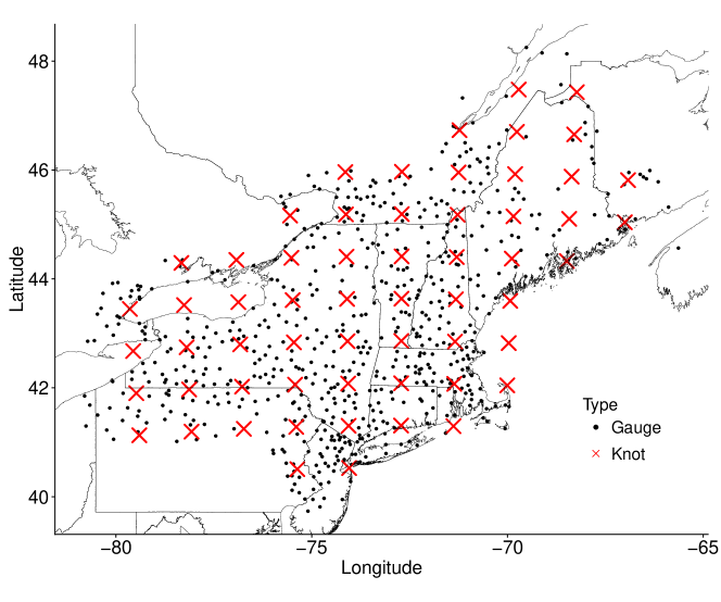
Figure 4: Precipitation gauge locations ($N=646$) across the northeastern United States and Canada are plotted as black dots and Gaussian density basis knot locations ($L=60$) are plotted as red crosses.

3.2 Model Fitting and Validation

The precipitation data are analyzed by applying the four max-id models described in Section 2, namely (M1) Gaussian density basis, $\theta=0$; (M2) Gaussian density basis, $\theta>0$; (M3) log-Gaussian process basis, $\theta=0$; and (M4) log-Gaussian process basis, $\theta>0$, where realizations of the process for each year are treated as i.i.d. replicates. Although further temporal dependence and trends could be modeled in both the GEV marginal parameters and basis scaling factors $A_{l,t}$, Kwiatkowski-Phillips-Schmidt-Shin tests (Kwiatkowski et al., 1992) for temporal non-stationarity among the annual maxima were performed separately for each station, and 85% of stations yielded no evidence for temporal non-stationarity at confidence level $95\%$. The proposed model would be more complex and computationally demanding to fit if one were to account for temporal non-stationarity. Therefore, for the sake of simplicity, and since overall the data do not appear to be highly non-stationary over time, we will ignore this aspect in our analysis. Accounting for temporal non-stationarity would be an interesting avenue of future research to further develop this model.

In particular, both the dependence model and GEV marginal distributions are assumed to be constant over time. We assume independent Gaussian process priors, each with constant mean $\beta_{\psi}\sim N(0,100)$ and stationary exponential covariance function $C(h)=\delta^{2}_{\psi}\exp(-h/\rho_{\psi}),h\geq 0$, $\psi\in\{\mu,\gamma\}$, on the location $\mu({\bm{s}})$ and log-scale $\gamma({\bm{s}})\equiv\log\{\sigma({\bm{s}})\}$ marginal parameters of the GEV distribution, with half-normal priors for $\delta^{2}_{\psi}\sim N_{+}(0,100)$ and $\rho_{\psi}\sim N_{+}(0,\max_{i,j}(||{\bm{s}}_{i}-{\bm{s}}_{j}||)^{2})$. Due to the difficulty in estimating the shape parameter (Cooley et al., 2007; Opitz et al., 2018), we use a spatially constant prior, $\xi\sim N(0,100)$. The dependence parameter priors are as follows: For $\alpha$ and $\theta$, we take $\alpha\sim{\rm Unif}(0,1)$ and $\theta\sim N_{+}(0,100)$. For the Gaussian density basis models, we use $L=60$ knot locations on an evenly spaced grid (see Figure 4). A half normal prior is put on the Gaussian density bandwidth parameter $\tau\sim N_{+}(0,\max_{i,j}(||{\bm{s}}_{i}-{\bm{s}}_{j}||)^{2})$. In the case of the log-Gaussian process basis models, we consider $L=10,15,$ and $20$ basis functions. More basis functions enable better representation of the data, but at the risk of overfitting. Priors $\delta_{K}^{2}\sim N_{+}(0,100)$ and $\rho_{K}\sim N_{+}(0,\max_{i,j}(||{\bm{s}}_{i}-{\bm{s}}_{j}||)^{2})$ are assumed for the exponential covariance parameters. Handling missing values is straightforward using the proposed approach. For each iteration of the MCMC algorithm, missing values are sampled from the posterior predictive distribution; this is detailed in the Supplementary Material. We run each MCMC chain under two different parameter initializations for 40,000 iterations using a burn-in of 10,000 with data from $546$ stations, reserving $100$ stations for model evaluation. Some of the parameters, particularly $\beta_{\mu}$ and $\beta_{\gamma}$, were quite slow to converge. In all four cases, the posterior densities were similar across the two initializations.

It is currently not possible to fit existing max-stable, inverted-max-stable (Wadsworth and Tawn, 2012), and other max-id models see, e.g. Huser et al., 2018, Padoan, 2013 using a full likelihood or Bayesian approach when the number of spatial locations is large; see Castruccio et al. (2016), Dombry et al. (2017) and Huser et al. (2019). Under these constraints, a natural alternative for comparison is the model for block maxima proposed by Sang and Gelfand (2010), which also belongs to the asymptotic independence class. Specifically, let $\{W({\bm{s}}),{\bm{s}}\in\mathcal{D}\}$ be a mean-zero Gaussian process with exponential correlation function and unit variance. The annual maxima are then modeled as $Z({\bm{s}})=\mathrm{GEV}^{-1}[\Phi\{W({\bm{s}})\};\mu({\bm{s}}),\sigma({\bm{s}}),\xi]$, where the location $\mu({\bm{s}})$ and $\log\{\sigma({\bm{s}})\}$ each follow mean zero Gaussian processes with exponential covariance functions, with the same priors as above, and $\Phi$ denotes the standard normal distribution function. We refer to this as the the GEV-Gaussian process copula model.

To compare models, we calculate out-of-sample log-scores (Gneiting and Raftery, 2007), for annual maxima at the 100 holdout stations, which is simply the log-likelihood of the holdout data for each model based on conditional predictive simulations of the latent model parameters at the unobserved sites. Since the log-scores are calculated on holdout data, they implicitly account for model complexity. We also emphasize that because the predictions are based on the joint likelihood, the log-scores reflect not only the marginal fits, but also how well the model captures the dependence characteristics of the observed data. The best log-score (higher scores are better) of the two initializations for each model is reported in Table 1. The max-id models ($\theta>0$) outperform their max-stable counterparts ($\theta=0$). The log-score for the GEV-Gaussian process copula model is worse than the other models considered. The estimated marginal surfaces are similar across all of the models considered, indicating that the misspecification is due to differences in the dependence model for the annual maxima.

The max-id, log-Gaussian process basis model with $\theta>0$ and $L=15$ basis functions has the highest log-score (shown in bold), suggesting it should be preferred among the considered models for this data application, and as such we focus on this model for the remainder of our analysis. For this model, the posterior mean (95% credible interval) estimates of the dependence parameters are $0.725\,\,(0.702,0.747)$ for $\alpha$, $0.024\,\,(0.006,0.060)$ for $\theta$, and for the spatial basis functions $33.9\,\,(23.8,47.2)$ for $\delta_{K}^{2}$ and $462\,\,(332,642)$ miles for $\rho_{K}$, suggesting the presence of some residual dependence beyond that explained by spatially-varying marginal parameters. Also, while we have specified vague priors on the model parameters, the posterior distributions are highly concentrated around their corresponding posterior means. Although the proposed inference scheme does not allow for jumps between $\theta=0$ and $\theta>0$, the posterior samples of $\theta$ are still somewhat informative about the asymptotic dependence class. In particular, since the dependence properties of our model are smooth in $\theta$ at zero, the fact that the 95% credible interval for $\theta$ is relatively symmetric and distant from 0 gives support for asymptotic independence among precipitation extremes.

To validate the decision of having the same dependence parameters $\alpha$ and $\theta$ over the entire region, log-Gaussian process basis models with $\theta>0$ were also separately fitted to four subregions, two inland and two coastal. The 95% credible intervals for $\alpha$ and $\theta$ overlap with those fitted to the entire region, suggesting homogeneous spatial dependence of the process over the study region.

Table 1: Log-scores estimated from annual maxima observed at the holdout stations are used to compare the four models presented in Section 2, and the GEV-Gaussian process copula model. Higher log-scores correspond to better fit. The max-id, log-Gaussian process basis model has the highest log-score (shown in bold).

	Gaussian Density Basis	log-Gaussian Process Basis			GEV-Gaussian Process Copula
L	60	10	15	20
$\theta=0$	-5292.5	-5410.7	-5406.4	-5415.2	-6097.048
$\theta>0$	-5218.3	-5194.6	-5172.6	-5207.9

Further, to examine the model fit, we compare empirical and model-based estimates of $\chi_{u}$ as a function of spatial lag $h$ and threshold $u$ for the holdout stations (Figure 5).

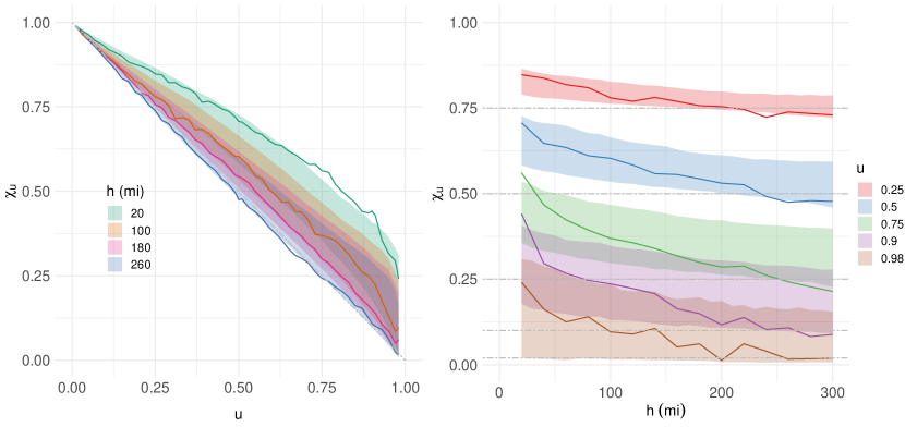
Figure 5: The left panel shows $\chi_{u}$ as a function of $u$ for fixed spatial lags $h=20,100,180,260$ miles calculated for the 100-holdout stations. Empirical estimates are shown as a solid black line, and max-id, log-Gaussian process basis model 95% credible intervals are shown as gray ribbons. The decay of $\chi_{u}$ towards zero as $u\rightarrow 1$ suggests that daily precipitation are asymptotically independent. To understand the spatial dependence of extreme precipitation at increasingly extreme levels, empirical (solid lines) and model 95% credible intervals (ribbons) of $\chi_{u}(h)$ for the holdout stations are plotted for several quantiles $u=0.25,0.5,0.75,0.9,0.98$ (right panel). Horizontal dash-dot gray lines representing the values of $\chi_{u}$ under an everywhere-independent model are plotted for reference. The plot shows good overall agreement between the model fits and empirical estimates.

The left panel shows $\chi_{u}$ as a function of $u$ for at fixed lags $h=20,100,180,260$ miles, and the right panel shows the spatial decay of $\chi_{u}$ as a function of spatial lag $h$ for several fixed marginal quantiles $u=0.25,0.5,0.75,0.9,0.98$. Empirical estimates are represented by solid lines and $95\%$ credible intervals for each model by shaded ribbons. From the left panel, we can see that the max-id model captures the asymptotic independence behavior of the precipitation data quite well. The max-stable model slightly underestimates the relatively strong dependence at shorter distances, but with comparable coverage to the max-id model at other distances (see Supplementary Material). The slight discrepancy at shorter distances may be due to the phenomenon described by Robins et al. (2000) wherein intervals from posterior summaries like $\chi_{u}$ that are calculated from MCMC draws are too narrow. From the right panel, we deduce that the annual maximum precipitation data exhibit quite strong spatial dependence up to about $200$ miles, with weaker spatial dependence at higher quantiles. Moreover, $\chi_{u}$ decays towards its independence level as a function of distance $h$ faster at the $0.9$ and $0.98$ quantiles than at the $0.25$ and $0.5$ quantiles.

In order to assess the joint spatial prediction skill of our model, we display in Figure 6 quantile-quantile (QQ)-plots for group-wise summaries of the annual maxima taken over the $100$ holdout stations (see Davison et al. (2012) for a similar analysis). The results show adequate correspondence between the model-based and empirical quantiles of the group-wise means, whereas the observed group-wise minima (maxima, respectively) appear to be slightly underestimated (overestimated, respectively) by the model. Corresponding QQ-plots when $\theta=0$ (not shown) give similar patterns with minima (maxima, respectively) lying slightly further above (below, respectively) the 95% credible intervals.

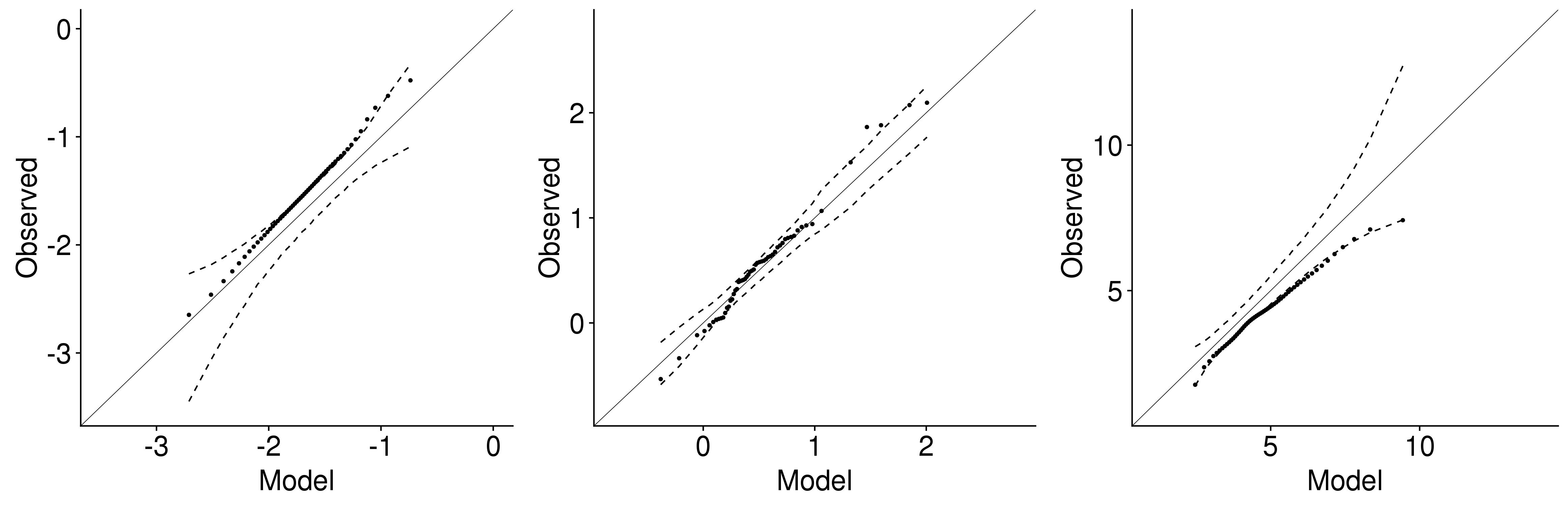
Figure 6: QQ-plots of the observed and predicted group-wise minima (left), mean (center), and maxima (right) taken over the annual maxima from all 100 holdout stations. The dashed lines represent 95% credible intervals. The plots reflect reasonable correspondence between the empirical and modeled multivariate distributions. To account for the fact that the marginal GEV distributions vary across stations, observations are first transformed to unit Gumbel scale using the probability integral transform for the GEV marginal distributions at each station from the fitted model.

Maps of the marginal posterior predictive means and standard deviations of the 0.99 quantile of annual maxima (i.e., 100-year return level) for the max-id, log-Gaussian process basis model are shown in Figure 7. The posterior mean surfaces are consistent with marginal quantile surfaces for the region as reported in NOAA Atlas 14 (Perica et al., 2013). The posterior standard deviation surface shows the greatest variability in Maine, Long Island, and along the boundary of the observation region where there are relatively few gauge locations. For illustration, observed maxima in 2012 and the posterior predictive mean for that year are plotted in Figure 8. Recall that only the scaling factors $A_{l,t}$ vary in time. The posterior predictive mean appears to capture the general spatial trend of the maxima observed in 2012 well.

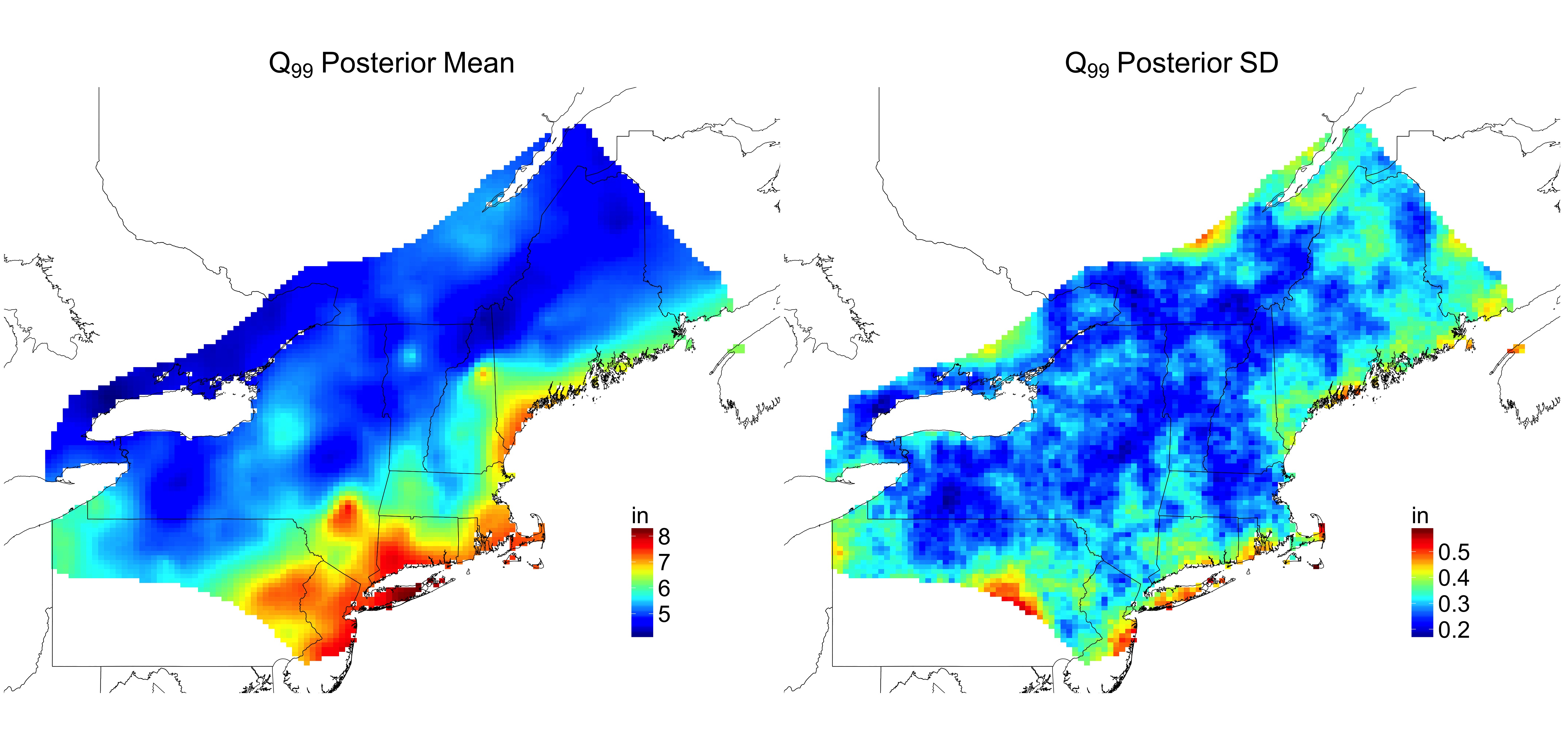
Figure 7: Pointwise posterior predictive mean (left) and standard deviation (right) of the 100-year return level of daily precipitation.

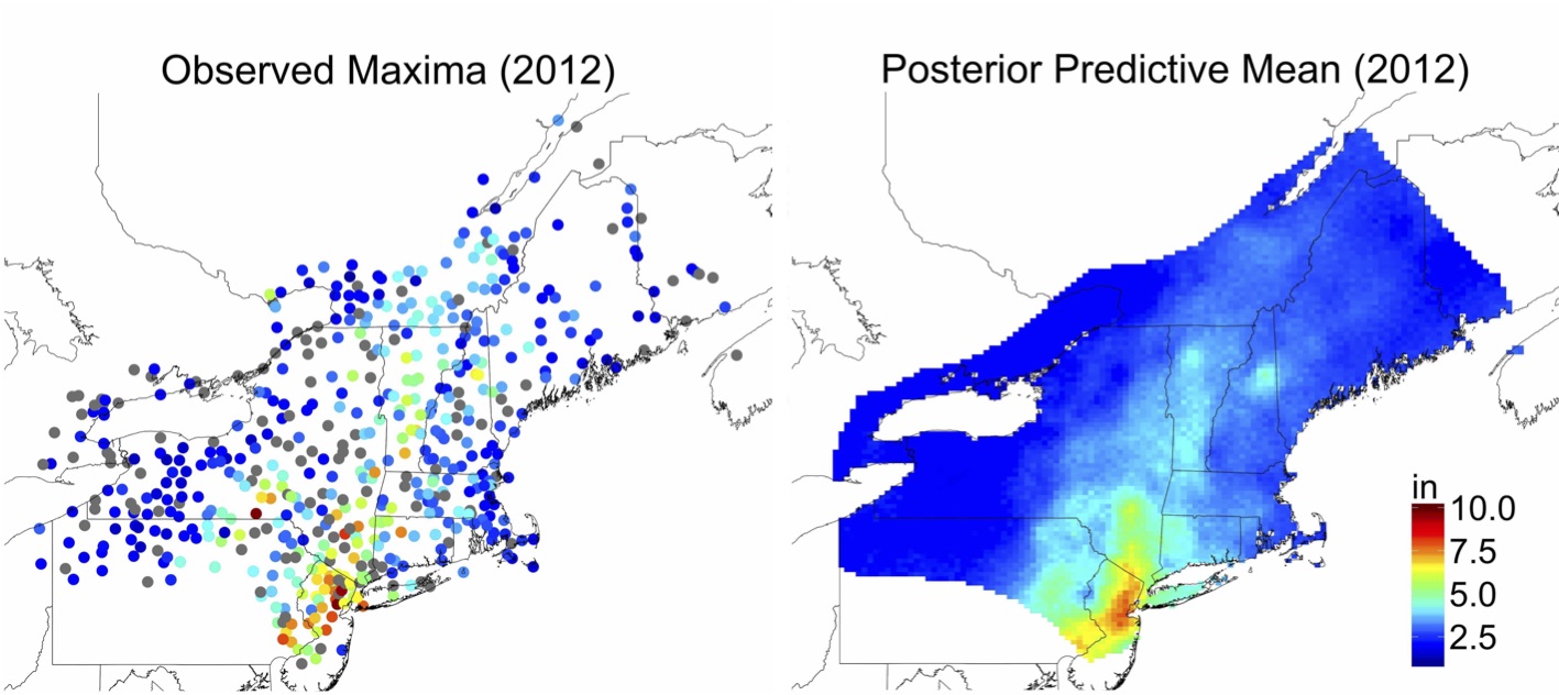
Figure 8: Observed precipitation accumulations (left), a single posterior predictive draw (middle), and posterior predictive means (right) for the year 2012. Missing values are shown in gray.

3.3 Principal Modes of Spatial Variability Among Precipitation Extremes

Spatial principal component analysis (PCA) (Demsar et al., 2013; Jolliffe, 2002) and Empirical Orthogonal Functions (Hannachi et al., 2007) have proven to be useful methods for exploring the main large scale features of spatial processes. However, aside from recent work by Morris (2016) and Cooley and Thibaud (2018), little has been done to this end for spatial extremes. The model we have proposed allows for an exploratory visualization that is very similar to a spatial PCA method that Demsar et al. (2013) refers to as Atmospheric Science PCA in their review of Spatial PCA methods, where the data consist of time replicates of a univariate spatial process observed at several locations.

An attractive feature of the log-Gaussian process basis model is that it provides a low-dimensional representation of the predominant modes of spatial variability among extremes. Analogously to factor analysis, the primary spatial trends among extreme precipitation can be described by a subset of the spatial basis functions $K_{l}({\bm{s}})$ that contribute the most to the overall process. To achieve this, motivated by PCA factorization, which finds the directions of maximum variance in the data, we rank the spatial basis functions $K_{l}({\bm{s}})$ $l=1,\ldots,L$, by the posterior year-to-year variation of their corresponding basis coefficients $A_{l,t}$ (i.e., higher posterior variance corresponds to lower rank). Arguably, both the means and variances of the coefficients $A_{l,t}$ play a role in the relative contribution of the corresponding basis function to the overall process. However, from inspection, the basis coefficients with the highest posterior variance also have the highest posterior means. Examining the variance of the basis coefficients for each $l=1,\ldots,L$, against their ranks give a rough indication of the number of basis functions with sizable contributions to the overall process. Also, while label switching is possible, from inspection of the MCMC samples of the basis functions, this does not appear to be a major concern for this application. If label switching is present, application of the pivotal reordering algorithm proposed by Marin et al. (2005); Marin and Robert (2007) can be used to permute the labels of the basis functions and scaling factors before ranking the basis functions. Posterior means of the first six spatial basis functions are shown in Figure 9. Most of the top ranked factor means in the $L=15$ basis function case were also identified as top ranked functions in the $L=10$ and $L=20$ case (see Supplementary Material).

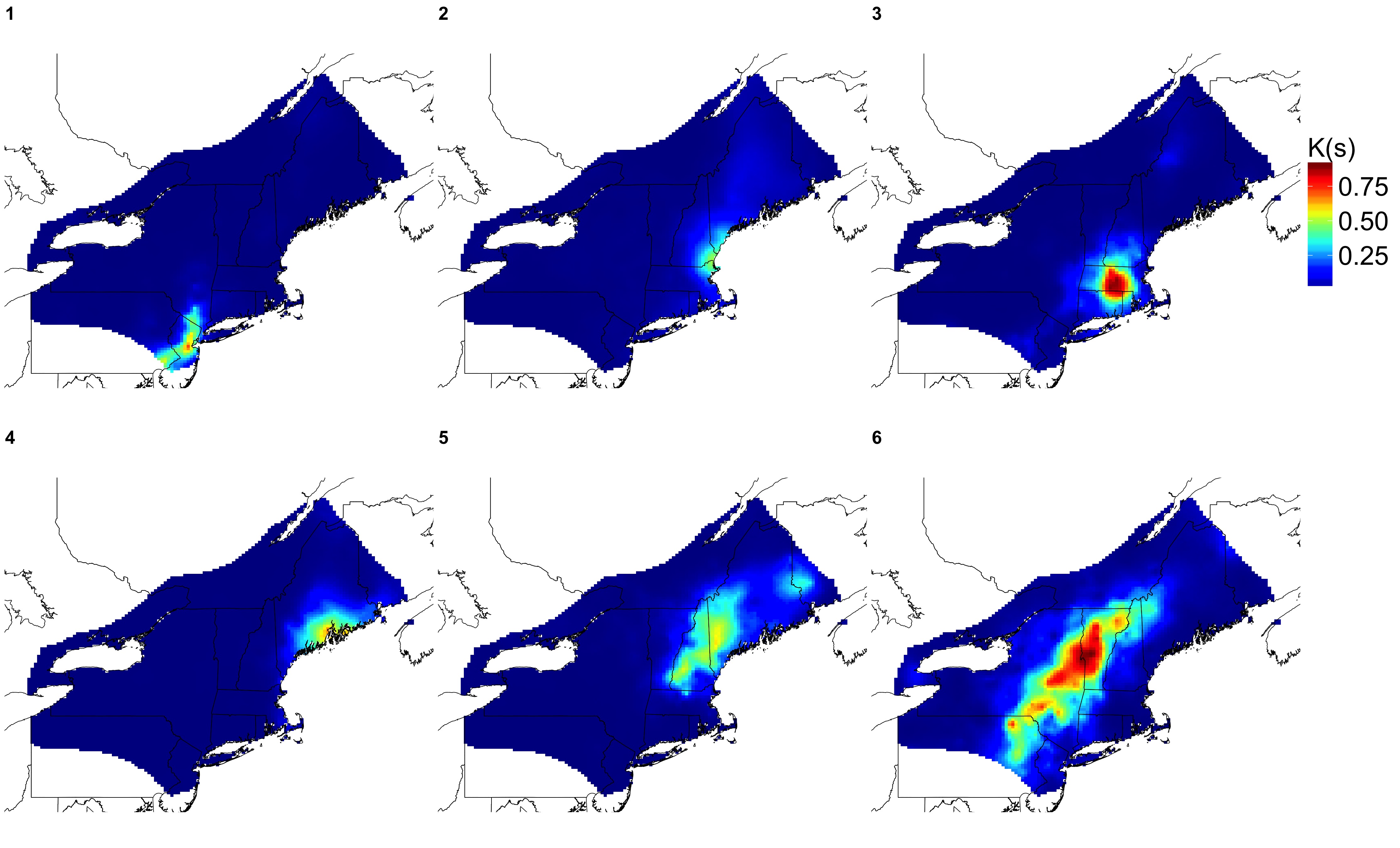
Figure 9: First six spatial basis functions ordered by the variance of their corresponding random basis coefficients from largest to smallest (left to right, top to bottom) for the $L=15$ basis function model. The year-to-year variation among the coefficients of these first six basis functions accounts for 97% of the total year-to-year variation among all of the basis coefficients. The shapes of the latent factors have reasonable interpretations in terms of geographic coastal and mountain features.

Unlike the pointwise marginal surfaces, which do not provide any information about the joint dependence of extremes, these basis functions capture spatial regions of simultaneous (in this case, merely the same year) extreme precipitation. The proportion of the total variation among the $A_{l,t}$ accounted for by variation in the coefficients of each of the first six basis functions is $0.48,0.33,0.07,0.04,0.03,$ and $0.02$ respectively. This does not imply that the top ranked factor is the dominating kernel $48\%$ of the time. Rather, if the variance of the scaling coefficients for the $l$th factor is high, then the year-to-year differences in the spatial modes of extremes should be well described by the peaks and troughs of the $l$th factor. For example, if $K_{l}({\bm{s}})$ has a peak around some location ${\bm{s}}^{*}$ then the conditional GEV distribution (given the factors and scaling coefficients) will be stochastically larger at ${\bm{s}}^{*}$ in years when $A_{l,t}$ is large and smaller when $A_{l,t}$ is small. Therefore, the low ranked factors describe regions where precipitation tends to be extreme together or more moderate together. The latent factors in Figure 9 have reasonable physical interpretations that are reflective of natural geographic features. In particular, they resemble observed patterns in extreme precipitation events occurring along the coast and mountain range borders. Just as with spatial PCA, we hesitate to make strong interpretations of the identified factors. However, the first four factors appear to correspond to coastal regions in New Jersey and New England that tend to be affected by the same localized tropical cyclones and convective storms. The last two modes appear to reflect the orographic effect of mountains in cloud formation, which cause moist air to rise.

4 DISCUSSION

In this paper, we extend the max-stable model for spatial extremes developed by Reich and Shaby (2012) in several ways. First, by using flexible log-Gaussian process basis functions, our model provides a more realistic low-dimensional factor representation that can be used to visualize the main modes of spatial variability among extremes. Second, our approach relaxes the rigid spatial dependence structure imposed by max-stable models, while possessing the positive dependence inherent to distributions for maxima. Inference on the tail dependence class is also possible, as our model can capture asymptotic independence when $\theta>0$, while having an asymptotically dependent, max-stable model on the boundary of the parameter space (when $\theta=0$).

We apply our model to extreme precipitation over the northeastern United States and Canada. Because it accounts for the spatial dependence among maxima and we are able to efficiently make conditional draws from our fitted model. The precipitation predictions from our model could be incorporated into a hydrological model for the flow path dynamics that incorporates factors like drainage basin topography, land use, and land cover to describe how precipitation falling over a common catchment translates into drainage and potential flooding. The precipitation analysis does not account for the cumulative effect of heavy precipitation over several days, which can overload an urban stormwater drainage system that is already operating at capacity. Further temporal modeling of the marginal distributions and space-time dependence characteristics would facilitate such an analysis; see, e.g., Huser and Davison (2014) for space-time modeling of precipitation extremes using max-stable processes.

For future work, adding a point mass at $\theta=0$ in the prior and proposal distributions would make it possible to account for model uncertainty and simultaneously perform model selection directly within the MCMC. Finally, while our focus in this paper has been on flexible sub-asymptotic modeling of maxima, another avenue for research is to investigate relaxing the rigid dependence structure of limiting generalized Pareto process models for peaks-over-threshold data (see, e.g., Castro Camilo and Huser, 2018; Huser and Wadsworth, 2019).

Appendix A Model Tail Dependence Properties

Since the marginal distributions of $Z({\bm{s}})$ are the same when constructed using the log-Gaussian process basis, $Z({\bm{s}}_{1})$ and $Z({\bm{s}}_{2})$ are asymptotically independent if ${\rm Pr}(Z({\bm{s}}_{1})>z|Z({\bm{s}}_{2})>z)\rightarrow 0$ as $z\rightarrow\infty$. The marginal distribution of the process at location ${\bm{s}}$ conditional on the basis functions is $G_{{\bm{s}}}\{z|K_{l}({\bm{s}}),l=1,\ldots L\}=\exp(L\theta^{\alpha}-\sum_{l=1}^{L}[\theta+\{{K_{l}({\bm{s}})/z}\}^{1/\alpha}]^{\alpha})$, and the joint distribution at two locations ${\bm{s}}_{1}$ and ${\bm{s}}_{2}$ is

$${\rm Pr}\{Z({\bm{s}}_{1})\leq z_{1},Z({\bm{s}}_{2})\leq z_{2}|K_{l}({\bm{s}}),l=1,\ldots L\}=\exp\left(L\theta^{\alpha}-\sum_{l=1}^{L}\left[\theta+\left\{{K_{l}({\bm{s}}_{1})\over z_{1}}\right\}^{1/\alpha}+\left\{{K_{l}({\bm{s}}_{2})\over z_{2}}\right\}^{1/\alpha}\right]^{\alpha}\right).$$

For brevity, we will drop the indices $l=1,\ldots L$, and write, e.g., $G_{{\bm{s}}}\{z|K_{l}({\bm{s}})\}\equiv G_{{\bm{s}}}\{z|K_{l}({\bm{s}}),l=1,\ldots L\}$. By $L^{\prime}Hospital$’s rule, we obtain

$$\chi({\bm{s}}_{1},{\bm{s}}_{2})|K_{l}({\bm{s}})=1+\underset{z\rightarrow\infty}{\lim}{{{\rm d}\over{\rm d}z}G_{{\bm{s}}_{1}}\{z|K_{l}({\bm{s}})\}\over{{\rm d}\over{\rm d}z}G_{{\bm{s}}_{2}}\{z|K_{l}({\bm{s}})\}}-\underset{z\rightarrow\infty}{\lim}{{{\rm d}\over{\rm d}z}\Pr\{Z({\bm{s}}_{1})\leq z,Z({\bm{s}}_{2})\leq z|K_{l}({\bm{s}})\}\over{{\rm d}\over{\rm d}z}G_{{\bm{s}}_{2}}\{z|K_{l}({\bm{s}})\}}$$

$$=2-\underset{z\rightarrow\infty}{\lim}{\Pr\{Z({\bm{s}}_{1})\leq z,Z({\bm{s}}_{2})\leq z|K_{l}({\bm{s}})\}\over G_{{\bm{s}}_{2}}\{z|K_{l}({\bm{s}})\}}\underset{z\rightarrow\infty}{\lim}{\sum_{l=1}^{L}\left[\theta+\left\{{K_{l}({\bm{s}}_{1})\over z}\right\}^{1/\alpha}+\left\{{K_{l}({\bm{s}}_{2})\over z}\right\}^{1/\alpha}\right]^{\alpha-1}\left\{K_{l}({\bm{s}}_{1})^{1/\alpha}+K_{l}({\bm{s}}_{2})^{1/\alpha}\right\}\over\sum_{l=1}^{L}\left[\theta+\left\{{K_{l}({\bm{s}}_{2})\over z}\right\}^{1/\alpha}\right]^{\alpha-1}K_{l}({\bm{s}}_{2})^{1/\alpha}}$$

$$=0$$

when $\theta>0$. Finally, by application of the Dominated Convergence Theorem, since $|\chi_{z}({\bm{s}}_{1},{\bm{s}}_{2})|K_{l}({\bm{s}})|<1$, we obtain $\chi({\bm{s}}_{1},{\bm{s}}_{2})={\rm E}\{\underset{z\rightarrow\infty}{\lim}\chi_{z}({\bm{s}}_{1},{\bm{s}}_{2})|K_{l}({\bm{s}})\}=0$ for all ${\bm{s}}_{1},{\bm{s}}_{2}\in\mathcal{S}$ For more detail, see the Supplementary Material.

In the case of $\theta=0$ and $\alpha<1$, Reich and Shaby (2012) showed that $Z({\bm{s}})\mid K_{l}({\bm{s}}),$ is max-stable with extremal coefficient $\theta_{2}({\bm{s}}_{1},{\bm{s}}_{2})\mid K_{l}({\bm{s}})=\sum_{l=1}^{L}\left[K_{l}({\bm{s}}_{1})^{1/\alpha}+K_{l}({\bm{s}}_{2})^{1/\alpha}\right]^{\alpha}$. Using the relation for max-stable processes with unit Fréchet margins that $\chi({\bm{s}}_{1},{\bm{s}}_{2})=2-\theta({\bm{s}}_{1},{\bm{s}}_{2})$, and by the Dominated Convergence Theorem, we have $\chi({\bm{s}}_{1},{\bm{s}}_{2})={\rm E}\{\underset{z\rightarrow\infty}{\lim}\chi_{z}({\bm{s}}_{1},{\bm{s}}_{2})|K_{l}({\bm{s}})\}=2-{\rm E}\{\theta_{2}({\bm{s}}_{1},{\bm{s}}_{2})\mid K_{l}({\bm{s}})\}=2-{\rm E}\{\sum_{l=1}^{L}\left[K_{l}({\bm{s}}_{1})^{1/\alpha}+K_{l}({\bm{s}}_{2})^{1/\alpha}\right]^{\alpha}\}>0$ when $\alpha<1$ for all ${\bm{s}}_{1},{\bm{s}}_{2}\in\mathcal{S}$. So, when $\theta=0$ and $\alpha<1$, $Z({\bm{s}})$ is asymptotically dependent, both conditionally on $K_{l},l=1,\ldots,L$ and unconditionally.

References

- Balkema and Resnick (1977) Balkema, A. A. and S. I. Resnick (1977). Max-infinite divisibility. Journal of Applied Probability 14(2), 309–319.
- Brown and Resnick (1977) Brown, B. M. and S. I. Resnick (1977). Extreme values of independent stochastic processes. Journal of Applied Probability 14(4), 732–739.
- Castro Camilo and Huser (2018) Castro Camilo, D. and R. Huser (2018). Local likelihood estimation of complex tail dependence structures, applied to U.S. precipitation extremes. arXiv preprint 1710.00875.
- Castruccio et al. (2016) Castruccio, S., R. Huser, and M. G. Genton (2016). High-order composite likelihood inference for max-stable distributions and processes. Journal of Computational and Graphical Statistics 25(4), 1212–1229.
- Coles et al. (1999) Coles, S., J. Heffernan, and J. Tawn (1999). Dependence measures for extreme value analyses. Extremes 2(4), 339.
- Cooley et al. (2007) Cooley, D., D. Nychka, and P. Naveau (2007). Bayesian spatial modeling of extreme precipitation return levels. Journal of the American Statistical Association 102(479), 824–840.
- Cooley and Thibaud (2018) Cooley, D. and E. Thibaud (2018). Decompositions of dependence for high-dimensional extremes. arXiv preprint 1612.07190.
- Crowder (1989) Crowder, M. (1989). A multivariate distribution with weibull connections. Journal of the Royal Statistical Society: Series B (Methodological) 51(1), 93–107.
- Davison and Huser (2015) Davison, A. C. and R. Huser (2015). Statistics of extremes. Annual Review of Statistics and Its Application 2, 203–235.
- Davison et al. (2013) Davison, A. C., R. Huser, and E. Thibaud (2013). Geostatistics of dependent and asymptotically independent extremes. Mathematical Geosciences 45(5), 511–529.
- Davison et al. (2019) Davison, A. C., R. Huser, and E. Thibaud (2019). Spatial extremes. In A. E. Gelfand, M. Fuentes, and R. L. Smith (Eds.), Handbook of Environmental and Ecological Statistics, pp. 711–744. CRC Press.
- Davison et al. (2012) Davison, A. C., S. A. Padoan, and M. Ribatet (2012). Statistical modeling of spatial extremes. Statistical Science. A Review Journal of the Institute of Mathematical Statistics 27(2), 161–186.
- de Haan and Ferreira (2006) de Haan, L. and A. Ferreira (2006). Extreme value theory. Springer Series in Operations Research and Financial Engineering. Springer, New York. An introduction.
- Demsar et al. (2013) Demsar, U., P. Harris, C. Brunsdon, A. S. Fotheringham, and S. McLoone (2013). Principal component analysis on spatial data: an overview. Annals of the Association of American Geographers 103(1), 106–128.
- Devroye (2009) Devroye, L. (2009). Random variate generation for exponentially and polynomially tilted stable distributions. ACM Transactions on Modeling and Computer Simulation (TOMACS) 19(4), 18.
- Dombry et al. (2017) Dombry, C., S. Engelke, and M. Oesting (2017). Bayesian inference for multivariate extreme value distributions. Electronic Journal of Statistics 11(2), 4813–4844.
- Dombry et al. (2013) Dombry, C., F. Éyi-Minko, and M. Ribatet (2013). Conditional simulation of max-stable processes. Biometrika 100(1), 111–124.
- Ferreira and de Haan (2014) Ferreira, A. and L. de Haan (2014). The generalized Pareto process; with a view towards application and simulation. Bernoulli. Official Journal of the Bernoulli Society for Mathematical Statistics and Probability 20(4), 1717–1737.
- Fougères et al. (2009) Fougères, A.-L., J. P. Nolan, and H. Rootzén (2009). Models for dependent extremes using stable mixtures. Scandinavian Journal of Statistics. Theory and Applications 36(1), 42–59.
- Gneiting and Raftery (2007) Gneiting, T. and A. E. Raftery (2007). Strictly proper scoring rules, prediction, and estimation. Journal of the American Statistical Association 102(477), 359–378.
- Hannachi et al. (2007) Hannachi, A., I. Jolliffe, and D. Stephenson (2007). Empirical orthogonal functions and related techniques in atmospheric science: A review. International journal of climatology 27(9), 1119–1152.
- Hougaard (1986) Hougaard, P. (1986). Survival models for heterogeneous populations derived from stable distributions. Biometrika 73(2), 387–396.
- Huser and Davison (2014) Huser, R. and A. C. Davison (2014). Space-time modelling of extreme events. Journal of the Royal Statistical Society. Series B. Statistical Methodology 76(2), 439–461.
- Huser et al. (2019) Huser, R., C. Dombry, M. Ribatet, and M. G. Genton (2019). Full likelihood inference for max-stable data. Stat 8, e218.
- Huser et al. (2017) Huser, R., T. Opitz, and E. Thibaud (2017). Bridging asymptotic independence and dependence in spatial extremes using Gaussian scale mixtures. Spatial Statistics 21(part A), 166–186.
- Huser et al. (2018) Huser, R., T. Opitz, and E. Thibaud (2018). Max-infinitely divisible models and inference for spatial extremes. arXiv preprint 1801.02946.
- Huser and Wadsworth (2019) Huser, R. and J. L. Wadsworth (2019). Modeling spatial processes with unknown extremal dependence class. Journal of the American Statistical Association 114, 434–444.
- Jolliffe (2002) Jolliffe, I. T. (2002). Principal component analysis (Second ed.). Springer Series in Statistics. Springer-Verlag, New York.
- Kabluchko and Schlather (2010) Kabluchko, Z. and M. Schlather (2010). Ergodic properties of max-infinitely divisible processes. Stochastic Processes and their Applications 120(3), 281–295.
- Kabluchko et al. (2009) Kabluchko, Z., M. Schlather, and L. de Haan (2009). Stationary max-stable fields associated to negative definite functions. The Annals of Probability 37(5), 2042–2065.
- Kabluchko and Stoev (2016) Kabluchko, Z. and S. Stoev (2016). Stochastic integral representations and classification of sum- and max-infinitely divisible processes. Bernoulli. Official Journal of the Bernoulli Society for Mathematical Statistics and Probability 22(1), 107–142.
- Kwiatkowski et al. (1992) Kwiatkowski, D., P. C. Phillips, P. Schmidt, and Y. Shin (1992). Testing the null hypothesis of stationarity against the alternative of a unit root: How sure are we that economic time series have a unit root? Journal of econometrics 54(1-3), 159–178.
- Marin et al. (2005) Marin, J.-M., K. Mengersen, and C. P. Robert (2005). Bayesian modelling and inference on mixtures of distributions. In Bayesian thinking: modeling and computation, Volume 25 of Handbook of Statistics, pp. 459–507. Elsevier/North-Holland, Amsterdam.
- Marin and Robert (2007) Marin, J.-M. and C. P. Robert (2007). Bayesian core: a practical approach to computational Bayesian statistics. Springer Texts in Statistics. Springer, New York.
- Morris (2016) Morris, S. A. (2016). Spatial Methods for Modeling Extreme and Rare Events. Thesis (Ph.D.) North Carolina State University.
- Opitz et al. (2018) Opitz, T., R. Huser, H. Bakka, and H. Rue (2018). INLA goes extreme: Bayesian tail regression for the estimation of high spatio-temporal quantiles. Extremes 21(3), 441–462.
- Padoan (2013) Padoan, S. A. (2013). Extreme dependence models based on event magnitude. Journal of Multivariate Analysis 122, 1–19.
- Perica et al. (2013) Perica, S., D. Martin, S. Pavlovic, I. Roy, M. S. Laurent, C. Trypaluk, D. Unruh, M. Yekta, and G. Bonnin (2013). Noaa atlas 14 volume 9 version 2, precipitation-frequency atlas of the united states, southeastern states. NOAA, National Weather Service 9, 18.
- Reich and Shaby (2012) Reich, B. J. and B. A. Shaby (2012). A hierarchical max-stable spatial model for extreme precipitation. The Annals of Applied Statistics 6(4), 1430–1451.
- Resnick (1987) Resnick, S. I. (1987). Extreme values, regular variation, and point processes, Volume 4 of Applied Probability. A Series of the Applied Probability Trust. Springer-Verlag, New York.
- Robins et al. (2000) Robins, J. M., A. van der Vaart, and V. Ventura (2000). Asymptotic distribution of values in composite null models. J. Amer. Statist. Assoc. 95(452), 1143–1167, 1171–1172. With comments and a rejoinder by the authors.
- Sang and Gelfand (2010) Sang, H. and A. E. Gelfand (2010). Continuous spatial process models for spatial extreme values. Journal of Agricultural, Biological, and Environmental Statistics 15(1), 49–65.
- Schlather and Tawn (2003) Schlather, M. and J. A. Tawn (2003). A dependence measure for multivariate and spatial extreme values: properties and inference. Biometrika 90(1), 139–156.
- Stephenson (2009) Stephenson, A. G. (2009). High-dimensional parametric modelling of multivariate extreme events. Australian & New Zealand Journal of Statistics 51(1), 77–88.
- Suro et al. (2009) Suro, T. P., G. D. Firda, and C. O. Szabo (2009). Flood of june 26-29, 2006, mohawk, delaware, and susquehanna river basins, new york. US Geological Survey Open-File Report 1063, 354.
- Tawn (1990) Tawn, J. A. (1990). Modelling multivariate extreme value distributions. Biometrika 77(2), 245–253.
- Thibaud and Opitz (2015) Thibaud, E. and T. Opitz (2015). Efficient inference and simulation for elliptical Pareto processes. Biometrika 102(4), 855–870.
- Wadsworth and Tawn (2012) Wadsworth, J. L. and J. A. Tawn (2012). Dependence modelling for spatial extremes. Biometrika 99(2), 253–272.