The Keck Lyman Continuum Spectroscopic Survey (KLCS):
the Emergent Ionizing Spectrum of Galaxies at $z\sim 3$

Abstract

We present results of a deep spectroscopic survey quantifying the statistics of the escape of hydrogen-ionizing photons from star-forming galaxies at $z\sim 3$. The Keck Lyman Continuum Spectroscopic Survey (KLCS) includes spectra of 124 galaxies with $\langle z\rangle=3.05\pm 0.18$ and $-22.1\leq M_{\rm uv}\leq-19.5$, observed in 9 independent fields, covering a common rest-wavelength range $880\leq\lambda_{0}/{\rm\textrm{\AA}}\lower 2.15277pt\hbox{$\;\buildrel<\over{\sim}\;$}1750$. We measure the ratio of ionizing to non-ionizing UV flux density $\langle f_{900}/f_{1500}\rangle_{\rm obs}$, where $f_{900}$ is the mean flux density evaluated over the range $\lambda_{0}=[880,910]$ Å. To quantify $\langle f_{900}/f_{1500}\rangle_{\rm out}$– the emergent ratio of ionizing to non-ionizing UV flux density – we use detailed Monte Carlo modeling of the opacity of H I in the intergalactic (IGM) and circumgalactic (CGM) medium as a function of source redshift. By analyzing high-S/N composite spectra formed from sub-samples exhibiting common observed properties and numbers sufficient to reduce the uncertainty in the IGM+CGM correction, we obtain precise values of $\langle f_{900}/f_{1500}\rangle_{\rm out}$, including a full-sample average $\mbox{$\langle f_{900}/f_{1500}\rangle_{\rm out}$}=0.057\pm 0.006$. We further show that $\langle f_{900}/f_{1500}\rangle_{\rm out}$ increases monotonically with $\rm Ly\alpha$ rest equivalent width $W_{\lambda}(\rm Ly\alpha)$, inducing an inverse correlation with UV luminosity as a by-product. To connect LyC leakage to intrinsic galaxy properties, we fit the composite spectra using stellar population synthesis (SPS) together with simple models of the ISM in which a fraction $f_{\rm c}$ of the stellar continuum is covered by optically-thick gas with column density $N_{\rm HI}$. We show that the composite spectra simultaneously constrain the intrinsic properties of the ionizing stars $(L_{900}/L_{1500})_{\rm int}$ along with $f_{\rm c}$, $N_{\rm HI}$, $E(B-V)$, and $\langle f_{\rm esc,abs}\rangle$, the escape fraction of ionizing photons. We find a sample-averaged $\mbox{$\langle f_{\rm esc,abs}\rangle$}=0.09\pm 0.01$, and that subsamples fall along a linear relation $\mbox{$\langle f_{\rm esc,abs}\rangle$}\simeq 0.75\langle W_{\lambda}(\rm Ly\alpha)/(110~{}\textrm{\AA})\rangle$ for $0\leq\langle W_{\lambda}(\rm Ly\alpha)\rangle\lower 2.15277pt\hbox{$\;\buildrel<\over{\sim}\;$}60$; subsamples with $\langle W_{\lambda}(\rm Ly\alpha)\rangle<0$ have $\langle f_{\rm esc,abs}\rangle$ consistent with zero. We use the FUV luminosity function, the distribution function $n[W_{\lambda}(\rm Ly\alpha)]$, and the relationship between $W_{\lambda}(\rm Ly\alpha)$ and $\langle f_{900}/f_{1500}\rangle_{\rm out}$ to estimate the total ionizing emissivity of $z\sim 3$ star-forming galaxies with $M_{\rm UV}\leq-19.5$: $\epsilon_{\rm LyC}\simeq 6\times 10^{24}$ ergs s^-1 Hz^-1 Mpc^-3. This value exceeds the contribution of QSOs by a factor of $\sim 1.2-3.7$, and accounts for $\lower 2.15277pt\hbox{$\;\buildrel>\over{\sim}\;$}50$% of the total $\epsilon_{\rm LyC}$ estimated using indirect methods at $z\sim 3$.

1. Introduction

Substantial recent efforts have focused on establishing the demographics of star-forming galaxies in the redshift range $6\lower 2.15277pt\hbox{$\;\buildrel<\over{\sim}\;$}z\lower 2.15277pt\hbox{$\;\buildrel<\over{\sim}\;$}10$ now believed to be most relevant for cosmic reionization (Planck Collaboration et al. 2016). Nevertheless, a detailed physical understanding of the reionization process remains elusive, due in large part to uncertainties that cannot be reduced simply by identifying a larger number of potential sources of ionizing photons. Crucial missing ingredients include knowledge of the intrinsic ionizing spectra of sources, and, more importantly, the net ionizing spectrum presented to the intergalactic medium (IGM) after passing through layers of gas and dust in the galaxy interstellar medium (ISM.) Unfortunately, these will be impossible to measure from direct photometric or spectroscopic study of reionization-era galaxies, even when the James Webb Space Telescope (JWST) comes on line, due to the rapidly increasing H I opacity with redshift along extended lines of sight to high redshifts, even post-reionization.

However, one can explore the likely behavior of Lyman continuum-producing objects, and perhaps make testable predictions, using observations of analogous sources at lower redshifts, where the opacity of intervening neutral H (H I) is less limiting, and where ancillary multiwavelength observations are more easily obtained. One avenue that has enjoyed recent success is ultraviolet (UV) observations conducted using Hubble Space Telescope (HST) of low-redshift galaxies that have been identified as likely analogs of the high redshift objects (e.g., Borthakur et al. 2014; Izotov et al. 2016a, b; Leitherer et al. 2016), such as ‘Lyman break analogs” (LBAs; Overzier et al. 2009), and “Green Peas” (Cardamone et al. 2009.) These objects, although rare in the present-day universe, have many of the same properties typical of high-redshift star-forming galaxies– e.g., high UV luminosity, strong nebular emission lines, strong galaxy-scale outflows, compact sizes, and high specific star formation rates (sSFRs). Alternatively, one can obtain very deep observations of larger samples of more distant galaxies, where direct observations of the Lyman continuum (LyC) are possible without necessarily observing from space (e.g., Steidel et al. 2001; Shapley et al. 2006; Iwata et al. 2009; Nestor et al. 2011; Vanzella et al. 2012; Nestor et al. 2013; Mostardi et al. 2013, 2015; Grazian et al. 2016.) Redshifts $z\lower 2.15277pt\hbox{$\;\buildrel>\over{\sim}\;$}3$ bring the rest-frame Lyman limit of hydrogen at 911.75 Å (13.6 eV) to observed wavelengths well above the atmospheric cutoff near 3100-3200 Å, where the atmosphere is transparent, the terrestrial background is darkest, and the instrumental sensitivity of spectrometers on large ground-based telescopes is high.

In general, ionizing photons produced by massive stars in H II regions are a local phenomenon, with a sphere of influence measured in pc; the “escape fraction” of ionizing photons from an isolated ionization-bounded H II region (i.e., where the ionized region is entirely embedded within a predominantly neutral region, and the extent of the H II region is determined by the production rate of ionizing photons) is zero, by definition. However, when the density of star formation is very high, as is often the case for high redshift star-forming systems, intense episodes of star formation and frequent supernovae can in principle produce ionized bubbles that carve channels through which Lyman continuum photons might escape unimpeded. The net escaping ionizing radiation depends on the geometry of the sites of massive star formation and the surrounding ISM, the lifetimes of the stars that produce the bulk of the ionizing photons (e.g., Ma et al. 2016), and the probability that during that lifetime favorable conditions for LyC photon escape will occur.

Once H-ionizing photons escape the ISM of a parent galaxy, the probability of detection by an observer at $z=0$ is governed by the effective opacity of intervening H I along the line of sight. This opacity increases steeply with redshift (e.g., Madau 1995; Steidel et al. 2001; Vanzella et al. 2010, 2012; Becker et al. 2015), and for the wavelength range most relevant to LyC measurement (i.e., $\lambda_{0}\lower 2.15277pt\hbox{$\;\buildrel<\over{\sim}\;$}912(1+z_{\rm s})$ for a source with redshift $z_{\rm s}$) it is also subject to large fluctuations from sightline to sightline, since it is dominated by the incidence of relatively small numbers of intervening H I systems with $16\lower 2.15277pt\hbox{$\;\buildrel<\over{\sim}\;$}{\rm log}~{}(N_{\rm HI}/{\rm cm}^{-2})\lower 2.15277pt\hbox{$\;\buildrel<\over{\sim}\;$}18$ (e.g., Rudie et al. 2013). As we discuss in more detail below (§7), these competing factors strongly favor the range $2.75\lower 2.15277pt\hbox{$\;\buildrel<\over{\sim}\;$}z\lower 2.15277pt\hbox{$\;\buildrel<\over{\sim}\;$}3.50$ for a ground-based survey.

Even within the optimal redshift range for ground-based observations, practical sensitivity limits impose severe restrictions on the dynamic range available for possible detections. The combination of limited sensitivity and detectability dominated by the stochastic behavior of the IGM foreground means that individual detections of LyC signal i.e., those for which significant LyC flux is detected without stacking) are almost guaranteed to be unusual either in their intrinsic properties, in having a fortuitously transparent line of sight through the IGM, or a combination of both. Direct detections of individual sources at high redshift (Vanzella et al. 2015; Shapley et al. 2016; Vanzella et al. 2017) are valuable for demonstrating that at least some galaxies produce ionizing radiation that propagates beyond their own ISM, but they do not place strong constraints on more typical galaxies.

In view of these challenges, successful characterization of the propensity for galaxies with particular common properties to “leak” LyC radiation requires observations of an ensemble, in order to marginalize over the fluctuations in the intervening IGM opacity. It should also include 1) the most sensitive possible measurements of individual sources, made as close as possible to the rest-frame Lyman limit of each; 2) a very accurate characterization of the statistics of intervening H I as a function of column density and redshift; 3) control over systematics – those affecting measurement of individual sources (e.g, background subtraction, contamination) and those that would invalidate the statistical IGM correction. The latter suggests observing sources in several independent survey fields and avoiding regions known to harbor unusual large-scale structures, if possible.

Although spectroscopic surveys at $z\sim 3$ using 8m-class telescopes first became feasible in the mid-1990s (e.g., Steidel et al. 1996, 2003), the initially-available instruments were not optimized for high near-UV/blue sensitivity as required for the most effective observations of LyC emission (Steidel et al. 2001). The situation changed substantially for the better with the commissioning on the Keck 1 telescope of the blue channel of the LRIS spectrograph (LRIS-B, Steidel et al. 2004) in 2002, followed by the installation of the Keck 1 Cassegrain Atmospheric Dispersion Corrector (Phillips et al. 2006) in 2007; projects demanding high efficiency in the wavelength range ($3100-4500$ Å) became much more feasible. Shapley et al. (2006) [S06], using pilot data obtained immediately following LRIS-B commissioning, presented what were apparently the first direct detections of LyC emission in the spectra of individual star-forming galaxies at $z\sim 3$. S06 observed a sample of 14 LBGs with LRIS in multi-slit mode for a total of $\sim 8$ hrs (in the mode sensitive to LyC light), reaching an unprecedented depth for individual galaxy spectra of $3\times 10^{-31}$ ergs s^-1 cm^-2 Hz^-1 at $\sim 3600$ Å (3$\sigma$ detection limit), corresponding to $AB\simeq 27.6$, or $\sim 20$ times fainter than the (non-ionizing) continuum flux density of L_∗ galaxies at $z\sim 3$. While the spectra presented by S06 were far superior for LyC detection compared to what had been available, it later turned out that 2 of the 3 putative detections of residual LyC flux were due to contamination of the LyC rest-frame spectral region by faint, unrelated foreground galaxies, based on subsequent near-IR spectra and HST imaging (Siana et al. 2015). In the years since, it has transpired that most apparent detections of significant LyC emission from $z\lower 2.15277pt\hbox{$\;\buildrel>\over{\sim}\;$}3$ galaxies have, on further inspection – particularly using high spatial resolution images obtained with HST – been attributed to similar foreground contamination (Vanzella et al. 2012, 2015; Siana et al. 2015; Mostardi et al. 2015).

Most of the more recent observational effort toward detecting LyC emission from intermediate and high redshift galaxies has been invested in imaging surveys, which have an obvious multiplex advantage, particularly when aimed at fields containing known galaxy over-densities. In such fields, narrow or intermediate band filters can be fine-tuned to lie just below the rest-frame Lyman limit at the redshift of interest (Inoue et al. 2005; Iwata et al. 2009; Nestor et al. 2011; Mostardi et al. 2013). Alternatively, one can use extremely deep broad-band UV images to search for LyC emission from galaxies having known spectroscopic redshifts that ensure the band lies entirely shortward of the rest-frame Lyman limit (Malkan et al. 2003; Cowie et al. 2009; Bridge et al. 2010; Siana et al. 2010; Rutkowski et al. 2016; Grazian et al. 2016, 2017). While imaging surveys obtain LyC measurements for every galaxy known or suspected to lie at high enough redshift in the field of view, putative detections (and the quantification of non-detections) requires both follow-up spectroscopy and/or high-resolution HST imaging (e.g., Vanzella et al. 2010; Nestor et al. 2013; Mostardi et al. 2015).

In the present work, we return to using very deep spectroscopic observations, similar to those presented by S06. The Keck Lyman Continuum Spectroscopic Survey (KLCS) expands and improves on the S06 study in several respects: first, the sample is larger by an order of magnitude, with a total of 136 $z\simeq 3$ galaxies observed. Second, the observations were conducted in 9 independent survey fields, which should drastically reduce the sample variance of the results, particularly if there are large-scale correlations in intergalactic LyC opacity that could have a very strong effect on results based on a single field (see discussion in S06.) Third, KLCS covers a broader range in both redshift ($2.72\leq z\leq 3.54$), and galaxy luminosity ($0.2<(L_{\rm uv}/L^{\ast}_{\rm uv})<3$) compared to S06. Most importantly, however, KLCS has benefited from the accumulated insight and lessons learned through experience – e.g., the importance of false positive detections due to foreground contamination and the sensitivity required for plausible detections – as well as from advances in the physical interpretation of the far-UV spectra of high redshift galaxies (e.g., Steidel et al. 2016; Eldridge et al. 2017) and in the precision of our statistical knowledge of the foreground IGM+CGM opacity (e.g., Rudie et al. 2013.)

In this paper, we show that, through careful control of systematics and concerted efforts to eliminate contamination, ensembles of deep rest-UV spectra can be used to measure the ratio of LyC flux density to non-ionizing UV flux density (hereafter $(f_{900}/f_{1500})_{\rm obs}$) with high precision. The KLCS observations provide individual galaxy spectra of unprecedented quality; composite spectra formed from substantial subsets provide templates that are the most sensitive ever obtained for similar high redshift objects, enabling access to a remarkable range of stellar, interstellar, and nebular spectral features, many of which have not been observed previously beyond the local universe. As well as direct constraints on the leakage of ionizing photons from galaxies, high quality rest-frame far-UV spectra encode the ancillary information on the massive star populations, the geometry and porosity of the ISM, the kinematics, physics, and chemistry of galaxy-scale outflows, and stellar and ionized gas-phase metallicities of the same galaxies – all of which are needed to place LyC leakage within the broader context of galaxies and the diffuse IGM.

The paper is organized as follows: §2 describes the selection of the KLCS sample; §3 details the spectroscopic observations, while §4 describes the data reduction, including the steps taken to minimize residual systematic errors in the sample. §5 defines the final KLCS sample used for subsequent analysis. LyC measurements from individual KLCS spectra are covered in §6. §7 describes modeling of the IGM and CGM transmission used to correct the KLCS LyC observations. In §8, we form a number of KLCS sub-samples and discuss the construction of their stacked (composite) spectra; §9 relates the composite spectra of the sub-samples to the corresponding LyC measurements, while §10 discusses the implications of the measurements. In §11 we evaluate the spectroscopic results in the context of a simple model for LyC escape and its connection to other observed galaxy properties, and propose the most appropriate method for calculating the total ionizing emissivity of the galaxy population at $z\sim 3$. Finally, §12 summarizes the principal results and discusses their broader implications and suggestions for future work. Appendix A summarizes data reduction steps taken to minimize residual systematic errors in KLCS as well as tests of their efficacy; Appendix B contains details of the IGM+CGM Monte Carlo transmission model used for the analysis.

Readers interested primarily in the results of the analysis, but not the details of the methods used to obtain them, may wish to focus on the final 4 sections (§9 - §12).

Where relevant, we assume a CDM cosmology with $\Omega_{\rm m}=0.3$, $\Omega_{\Lambda}=0.7$, and $h=0.7$. All spectroscopic flux density measurements used in the paper are expressed as flux per unit frequency ($f_{\nu}$), and are generally plotted as a function of wavelength, so that a spectrum with constant $f_{\nu}$, constant $m_{\rm AB}$, or $f_{\lambda}\propto\lambda^{-\beta}$ with $\beta=2$, appears “flat”.

2. The KLCS Sample

2.1. Target Redshift Range

Ozone in the Earth’s atmosphere efficiently blocks ultraviolet (UV) radiation with a sharp transparency cutoff preventing photons with $\lambda\leq 3100$ Å (at elevation of 4200m, as on Mauna Kea) from reaching the surface. A consequence is that ground-based observations of rest-frame LyC photons from celestial objects require observing them at redshifts $z\lower 2.15277pt\hbox{$\;\buildrel>\over{\sim}\;$}2.725$, where the rest-frame Lyman limit of H I ($\lambda_{0}=911.75$ Å) falls at an observed wavelength of $\simeq 3400$ Å. At higher redshifts, observations of the rest-frame LyC benefit from the generally higher instrumental throughput and atmospheric transmission at longer wavelengths, but the sensitivity for detection of LyC flux escaping from galaxies actually declines precipitously with increasing redshift beyond $z\simeq 3.5$ (e.g., Madau 1995; Steidel et al. 2001; Vanzella et al. 2010; see §7)

The decreasing sensitivity with increasing redshift is due to a combination of several effects: first and most obviously, galaxies of a given intrinsic UV luminosity ($L_{\rm uv}$) become apparently fainter with redshift; in addition the characteristic $L^{\ast}_{\rm uv}(z)$ itself dims as redshift increases beyond $z\sim 3$ (e.g., Reddy & Steidel 2009; Bouwens et al. 2010; Finkelstein et al. 2015). Although the net instrumental sensitivity at wavelengths $912(1+z_{\rm s})$ Å increases with redshift from $z\sim 2.7$ to $z\sim 3.5$, at redshifts $z\lower 2.15277pt\hbox{$\;\buildrel>\over{\sim}\;$}3.5$ the throughput gains are more than offset by the increasing intensity of the sky background against which any faint LyC signal must be measured.

Most importantly, line and continuum opacity of neutral hydrogen (H I) in the IGM along the line of sight increases steeply with $z_{\rm s}$ (e.g., Madau 1995). Even if intergalactic H I contributed no net continuum opacity for ionizing photons emitted from a source with $z_{\rm s}$, the LyC region will be blanketed by the effective opacity caused by Lyman series lines with $z\lower 2.15277pt\hbox{$\;\buildrel<\over{\sim}\;$}911.8/1215.7\times(1+z_{\rm s})^{-1}$, reducing the dynamic range accessible to LyC detection. When one includes the net LyC opacity contributed by gas outside of the galaxy, but at redshifts near enough to $z_{\rm s}$ to impact the net transmission averaged over the LyC detection band, the median transmission in the rest-wavelength interval 880–910 Å decreases by a factor of $\simeq 7$ between $z=3$ and $z=5$, (see discussion in §7, and Table 12.)

Tallying all of the exacerbating factors, the overall difficulty of a (ground-based) detection of LyC signal from a $L_{\rm uv}=L_{\rm uv}^{\ast}(z_{\rm s})$ increases by a factor of $\sim 35$ as one moves from $z\sim 3$ to $z\sim 5$. Thus, there is strong impetus for a ground-based LyC survey to focus on sources with $2.75\lower 2.15277pt\hbox{$\;\buildrel<\over{\sim}\;$}z_{\rm s}\lower 2.15277pt\hbox{$\;\buildrel<\over{\sim}\;$}3.5$, as we have done for KLCS.

2.2. Survey Design

Targets for KLCS were selected in 9 separate fields on the sky (Table 1), chosen from among $\simeq 25$ high latitude fields in which we have obtained deep $U_{\rm n}G{\cal R}$ photometry suitable for selecting LBG candidates at $z\sim 3$ (see Reddy et al. 2012 for a nearly-complete list) as well as spectroscopic follow-up observations. The final field selection was based on a combination of visibility time at low airmass during scheduled observing runs and the number of galaxies with previously-obtained spectroscopic redshifts in the range $2.9\lower 2.15277pt\hbox{$\;\buildrel<\over{\sim}\;$}z\lower 2.15277pt\hbox{$\;\buildrel<\over{\sim}\;$}3.2$ that could be accommodated on a single slit mask of the Low Resolution Imaging Spectrometer (LRIS; Oke et al. 1995; Steidel et al. 2004) on the Keck 1 telescope. For six of the nine KLCS fields (see Table 1), selection of star-forming galaxy candidates using rest-UV continuum photometry was performed during the course of a survey for $z\sim 3$ Lyman-break galaxies (LBGs; see Steidel et al. 2003). Three additional fields (Q0100$+$1300, Q1009$+$2956 and HS1549$+$1919) including $z\sim 3$ LBGs were observed during the period 2003 to 2009; these comprise part of the Keck Baryonic Structure Survey (KBSS; Steidel et al. 2004, 2010; Rudie et al. 2012; Steidel et al. 2014; Strom et al. 2017.)

Selection of $z\sim 3$ LBGs in all 9 of the KLCS fields was based on photometric selection using the 3-band ($U_{n}G{\cal R}$) photometric system described in detail by Steidel et al. (2003); photometric and spectroscopic catalogs for 6 of these fields (as of 2003) were also presented in that work. Full photometric and spectroscopic survey catalogs for the 3 KBSS fields will be presented elsewhere.

Table 1Keck Lyman Continuum Spectroscopic Survey: Observations

Field	RA (J2000)	Dec (J2000)	Mask	$N_{\rm obs}$	$N$	$N_{\rm det}$	Date Observed	ADC	$t_{\rm exp}$
Q0100$+$1300	01:03:11.27	$+$13:16:18.0	q0100_L1	15	12	0	2006 Dec	no	5.1
			q0100_L2	$\cdots$	$\cdots$	$\cdots$	2007 Sep	yes	5.2
Q0256$-$000	02:59:05.13	$+$00:11:06.8	q0256_L1	15	11	0	2007 Nov	yes	8.5
B20902$+$34	09:05:31.23	$+$34:08:01.7	b20902_L1	14	11	0	2007 Nov	yes	5.0
			b20902_L1	$\cdots$	$\cdots$	$\cdots$	2008 Apr	yes	3.4
Q0933$+$2854	09:33:36.09	$+$28:45:34.8	q0933_L2	13	10	1	2007 Mar	yes	9.2
			q0933_L3	15	14	3	2008 Apr	yes	8.2
Q1009$+$2956	10:11:54.49	$+$29:41:33.5	q1009_L1	12	11	0	2006 Dec	no	7.0
Westphal	14:17:43.21	$+$52:28:48.5	gws_L1	15	15	3	2008 Jun	yes	8.5
Q1422$+$2309	14:24:36.98	$+$22:53:49.6	q1422_L2	16	15	3	2008 Apr	yes	8.2
HS1549$+$1919	15:51:54.75	$+$19:10:48.0	q1549_L2	13	13	2	2008 Apr	yes	4.3
			q1549_L2	$\cdots$	$\cdots$	$\cdots$	2008 Jun	yes	4.2
DSF2237b	22:39:34.10	$+$11:51:38.8	dsf2237b_L1	14	14	3	2007 Sep	yes	7.3
			dsf2237b_L1	$\cdots$	$\cdots$	$\cdots$	2007 Nov	yes	5.5
TOTAL			10	136	124	15			89.6

We used a slitmask design strategy that assigned highest priority to comparatively brighter (${\cal R}\leq 24.5$) LBGs known to have redshifts in the interval $2.9\leq z\leq 3.3$. Other star-forming galaxies in a broader redshift range $2.7<z<3.6$ were assigned somewhat lower priority. If space on a mask was still available, we included additional candidates that were identically selected but had not been previously observed spectroscopically. Objects that had already been classified as AGN based on their existing survey spectra were deliberately given relatively high priority in the KLCS mask design, as little is known about whether ionizing radiation escapes from low-luminosity AGN or QSOs. This small sub-sample will be addressed in future work.

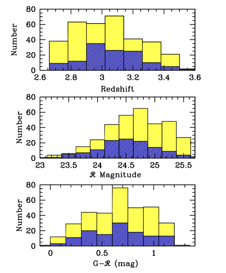
Figure 1.— The distribution of redshift (top), ${\cal R}$ magnitude (center), and $G-{\cal R}$ color for the KLCS sample (dark shaded histograms) as compared with those of all confirmed LBGs in the 9 survey fields used (light shaded histograms). Apart from the slight preference for brighter objects (${\cal R}\lower 2.15277pt\hbox{$\;\buildrel<\over{\sim}\;$}25$) and for objects at redshift $z\sim 3.0$, the KLCS sample is not significantly biased with respect to the LBG population.

Figure 1 presents comparisons between the parent sample from which targets were selected (light histograms), and those that were successfully observed (dark histograms), in terms of redshift, apparent magnitude ${\cal R}$, and color $G-{\cal R}$. The “parent” sample in this case includes all galaxies with redshifts $2.7<z<3.6$ located in the same set of fields used in the KLCS. The middle panel of Figure 1 shows that the KLCS sample has a moderate excess of sources with ${\cal R}<24.5$ and a related deficiency of galaxies with $25.0\leq{\cal R}\leq 25.5$, which is an expected consequence of our observing strategy. The redshift distribution of KLCS galaxies also demonstrates our slight preference for targets in $2.9\leq z\leq 3.2$ redshift “window”. We find no difference in the distribution of $G-{\cal R}$ color between KLCS and all spectroscopically identified galaxies in these fields (Figure 1, bottom panel). Thus, the sub-sample of galaxies observed for the KLCS is slightly brighter, and has a slightly tighter redshift distribution, than the LBGs in the same fields, but is otherwise representative.

3. Spectroscopic Observations

As summarized in Table 1, a total of 136 galaxies was observed, in 9 independent fields using 10 different slitmasks. Of the galaxies observed, 13 were later excluded from the LyC analysis because of uncalibrated slit defects, close companions on the slit, scattered light, or other potential sources of systematic error that would make LyC flux measurements less secure (see the detailed discussion in §5 below).

All 10 slitmasks were designed with $1\mbox{${}^{\prime\prime}\mskip-7.6mu.\,$}2$ slit widths and individual slit lengths between 10″and 30″; the median slit length for high priority KLCS targets was 20″. With the exception of the Q0933$+$2854 field, a single slitmask was observed in each field, containing between 8 and 16 objects known to lie at redshifts $2.7<z<3.6$. The observations were conducted over the course of 6 separate observing runs using LRIS on the Keck 1 10m telescope between 2006 December and 2008 June. As summarized in Table 1, the total integration time per slitmask was between 8.2 and 12.8 hours. Fields were generally observed within 2 hours of the meridian in order to minimize attenuation by atmospheric extinction and (in the case of the observations made prior to 2007 August) slit losses due to differential atmospheric refraction.

All observations were made using the same configuration of the LRIS double-beamed spectrograph (Oke et al. 1995; Steidel et al. 2004), with the incoming beam divided near 5000 Å using the “d500” dichroic beamsplitter. Wavelengths shortward of 5000 Å were recorded by the “blue” spectrograph channel (LRIS-B) and those longward of $\simeq 5000$ Å by the red channel (LRIS-R). LRIS-B was configured with a 400 line/mm grism with first-order blaze at 3400 Å, providing wavelength coverage from 3100 Å to beyond the dichroic split near 5000Å. The LRIS-B detector was binned 1x2 (binned in the dispersion direction) at readout in order to minimize the effect of read noise, which for these devices is $\simeq 3.8$e^- pix^-1, resulting in pixels that project to 0${}^{\prime\prime}\mskip-7.6mu.\,$135 on the sky in the spatial direction and $\simeq 2.18$ Å per pixel in the dispersion direction. LRIS-R was configured with a 600 line/mm grating with first-order blaze at 5000 Å, with spectra recorded using the (pre-2009) Tektronix 2k x 2k (monolithic) detector with 24 $\mu$m pixels. With no on-chip binning, the scale at the detector was 0${}^{\prime\prime}\mskip-7.6mu.\,$211 per pixel spatially and 1.28 Å pix^-1 in the dispersion direction. The LRIS-R grating was tilted such that all KLCS slits would have wavelength coverage from shortward of the dichroic split to $\lower 2.15277pt\hbox{$\;\buildrel>\over{\sim}\;$}7000$ Å depending on the spatial position of the slit within the LRIS field of view.

Individual exposure times were $1800$s and all LRIS-B and LRIS-R exposures were obtained simultaneously, resulting in identical observing conditions and integration times for a given mask. Data were collected under mostly photometric observing conditions, and all data used in the KLCS were obtained with seeing $<1$${}^{\prime\prime}\mskip-7.6mu.\,$0, and typically $\lower 2.15277pt\hbox{$\;\buildrel<\over{\sim}\;$}0$${}^{\prime\prime}\mskip-7.6mu.\,$7.

Prior to the commissioning of the Keck 1 Cassegrain Atmospheric Dispersion Corrector (ADC; Phillips et al. 2006) in the summer of 2007, all KLCS observations were obtained at elevations within $30^{\circ}$ of zenith and position angle close to the parallactic in order to minimize effects of differential refraction. Once commissioned, the ADC was used for all observations, greatly enhancing the efficiency of the survey by allowing position angle to be unconstrained during mask design, thus allowing inclusion of a larger number of high priority targets. By correcting differential refraction before the slitmask, the ADC improved the data quality particularly for LRIS-B, and enables the use of simpler (and more robust) data reduction and extraction techniques (see §4.2).

The spectral resolution achieved varied slightly depending on observing conditions and the angular size of objects within each slit. With a typical seeing-convolved profile size of FWHM$\simeq 0\mbox{${}^{\prime\prime}\mskip-7.6mu.\,$}8-0\mbox{${}^{\prime\prime}\mskip-7.6mu.\,$}9$ for Lyman-break galaxies at $z\sim 3$ (Law et al. 2007, 2011), the average resolving power is $R\simeq 800$ (LRIS-B) and $R\simeq 1400$ (LRIS-R) with the dispersers described above (see Steidel et al. 2010).

The dichroic split at 5000 Å typically places the location of $\rm Ly\alpha$, i.e. $1215.67(1+z_{\rm s})$ Å, near the transition wavelength between the spectral channels for $z\sim 3$. Longward of $\rm Ly\alpha$ our primary objective was to resolve the width of typical interstellar absorption lines (FWHM$\simeq 500-700$ km s${}^{-1}\,$; see, e.g., Pettini et al. 2002; Shapley et al. 2006; Steidel et al. 2010) so that the degeneracy between velocity width and covering fraction could be disentangled. The FWHM$\simeq 200$ km s${}^{-1}\,$ resolution provided by the 600/5000 grating represented a compromise between resolution and sensitivity. For LRIS-B, high sensitivity (particularly in the wavelength range 3400-4000 Å) was of paramount importance, hence the choice of the 400/3400 grism, which in combination with the LRIS-B optics produces very high UV/blue throughput (see Steidel et al. 2004). The spectral resolution of FWHM $\simeq 375$ km s${}^{-1}\,$ is modest, but still adequate to resolve typical strong absorption and emission lines.

4. Calibrations and Data Reductions

4.1. Calibrations

We obtained spectroscopic flat-field calibration images for LRIS-R and LRIS-B separately. Internal halogen lamp spectra provided adequate flat-fields for all LRIS-R data, but were not suitable for LRIS-B, which for our configuration requires very good flats particularly in the wavelength range 3100-4000 Å, where there are substantial spatial variations in quantum efficiency due to non-uniformities in the thinning of the silicon during manufacture.

We found from experience (for LRIS-B) that slitmask spectra of the twilight sky, obtained at similar elevation and instrument rotator angle to the science observations through the same mask, are the most effective solution; these were obtained at the beginning and end of each observing night. The twilight sky spectral flats produce adequate signal in the UV, but record the scattered solar spectrum rather than a featureless continuum. To remove the G-star spectrum but preserve the pixel-to-pixel sensitivity variations, we divide the raw flats by a spatially median-filtered 1-d spectrum calculated at regular intervals along each slit, producing images normalized to an average value of unity but retaining the desired pixel-to-pixel sensitivity variations. The issue of scattered light associated with flat fielding is addressed in §A.1 below.

Internal arc lamp spectra (Hg, Ne, Zn, and Cd for LRIS-B, Hg, Ne, Ar, Zn for LRIS-R) were used for wavelength calibration for both LRIS-B and LRIS-R, with 5th order polynomial fits resulting in typical residuals of $\simeq 0.10$ Å  and $\simeq 0.07$ Å for LRIS-B and LRIS-R, respectively. The arc-based wavelength solutions were subsequently shifted by small amounts using measurements of night sky emission lines recorded in each science exposure.

Spectrophotometric standard stars from the list of Massey et al. (1988) were observed at the end of each night through $1\mbox{${}^{\prime\prime}\mskip-7.6mu.\,$}0$ slit oriented at the parallactic angle (for all observations, both pre- and post-installation of the ADC in August 2007), with configuration settings otherwise identical to mask observations. Absolute flux calibration uncertainties are estimated to be of order $\simeq 20$% due to potential variations in seeing conditions (and the associated variation in slit losses) between slitmask and standard star observations. However, red-side and blue-side exposures were always obtained simultaneously, for both science and standard star observations, so that with careful reductions of the standards, the relative spectrophotometry between the blue and red channels is much more precise than the absolute spectrophotometry; the latter is relatively unimportant to our analysis (see §4.2 below).

4.2. Data Reduction

The standard LRIS spectroscopic data processing pipeline we have used for previous surveys with LRIS (e.g., Steidel et al. 2003, 2004, 2010) was generally followed in processing KLCS LRIS-R data. However, given the challenge of measuring very faint flux densities at levels well below the sky background in the LyC region, we paid particular attention to developing procedures for LRIS-B reductions with a goal of minimizing residual systematic errors wherever possible. Given the potential importance of systematics to the final LyC results, we describe the details of the reduction procedures up to the extraction of 1-D spectra in Appendix A.

The 2-D, background-subtracted, stacked spectrograms for each sequence of LRIS-B or LRIS-R observations with a given slitmask were reduced (as described in Appendix A) so that the centroid of the trace for a given object on the slit lies at a constant spatial pixel along the dispersion direction, whether or not the observation was made using the ADC. We adopted, conservatively, a 1${}^{\prime\prime}\mskip-7.6mu.\,$35 boxcar extraction window (10 spatial pixels on the LRIS-B detector) to avoid making assumptions about variations of the spatial profile with wavelength – particularly when the trace extends to wavelengths beyond where there is obvious detected flux. Thus, the extraction aperture for every object is a rectangular region of size 1${}^{\prime\prime}\mskip-7.6mu.\,$2 by 1${}^{\prime\prime}\mskip-7.6mu.\,$35 on the sky.

For each extracted 1-D spectrum, we used an identical extraction region on the 2-D “sky + object” 2-D spectrograms described above (§A.5.1), i.e.,

$$S[i]=\sum_{j=k-5}^{k+5}s[i,j]$$ (1)

and

$$\sigma[i]=\left(\sum_{j=k-5}^{k+5}\sigma_{\rm pix}^{2}[i,j]\right)^{0.5}~{},$$ (2)

where $k$ is the spatial position (in $j$ pixels) of the object trace, $S[i]$ is the resulting 1-D spectrum at dispersion point $[i]$, and $\sigma[i]$ is the corresponding one-dimensional error vector. Section A.6 describes in more detail the extent to which the noise model agrees with the data.

Mask data sets obtained on more than one observing run (see Table 1) were reduced to 1-D separately, and then combined using inverse variance weighting to produce final 1-D spectra. The 1-D spectra were wavelength calibrated using the 1-D arc spectra extracted from the same region of the processed 2-D arc frames, zero-pointed using night sky emission lines measured in the extracted 1-D object+sky spectra (§A.5.1) to correct for small amounts of flexure and slight differences in illumination between the internal arc lamps and the night sky. The final LRIS-B wavelength scales are in the vacuum, heliocentric frame with a linear dispersion of 2.14 Å ${\rm pix}^{-1}$ (LRIS-B), covering 3200-5000 Å.

Finally, the extracted LRIS-B and LRIS-R spectra were flux calibrated using standard stars from the list of Massey et al. (1988), obtained on the same night as the data comprising each 1-D extracted science spectrum, and corrected for Galactic extinction assuming the reddening maps of Schlegel et al. (1998). The standard star observations on the blue and red sides were made simultaneously, with the slit oriented at the parallactic angle. Because the LRIS long slit lies at a fixed position in the field of view of the instrument, the sensitivity curves in the wavelength transition region of the dichroic beamsplitter (where the spectral response of the interference coatings change rapidly with increasing wavelength from reflection to transmission) are not perfectly matched for slits located far from the focal plane position of the longslit, due to small differences in angle of incidence of the incoming light. However, through experimentation we found that accurate relative spectrophotometry could be achieved by using only LRIS-B spectra for $\lambda<5000$ Å and only LRIS-R spectra for $\lambda>5000$ Å; i.e., without averaging over the region of overlap.

Continuous LRIS-B+R spectra, covering 3200-7200 Å  were produced by remapping the individual calibrated spectra onto a linear wavelength scale chosen so as to preserve the spectral sampling of the higher resolution red-side data, 1.0 Å ${\rm pix}^{-1}$. These were used to produce composite spectra using subsets of the KLCS sample (§8.) Thus, we made final 1-D flux calibrated spectra for each source.

5. Defining the KLCS Sample for Analysis

In addition to the procedures described above to ensure that the observed sample is as free as possible from background subtraction systematics, we carefully examined all stacked 2-D spectrograms and extracted 1-D spectra for the sample of 136 observed galaxies to check for remaining issues that might compromise measurements of residual LyC flux. The following criteria were considered serious enough to warrant removing galaxies from the analysis sample:

1) Instrumental defects were apparent in the two-dimensional spectrograms. As discussed above, the effects of non-uniform scattered light (§A.1) and/or irreparable slit illumination irregularities (§A.3) can negatively impact the quality of the flat-fielding and background subtraction stages. There were 5 cases in which such effects were judged to be relevant, 1 in each of the Q0100, Q0256, and B20902 fields, and 2 on mask q0933_L2 (pre-ADC) in the Q0933 field; all 5 were removed from the KLCS analysis sample.

2) The primary target galaxy appeared to have another object near enough on the slit that the light from the two objects could not be separated with confidence in the 1-D extraction; 3 such cases were identified (one object from each of Q0100, B20902, and Q0933 [mask q0933_L2]), and removed from the sample.

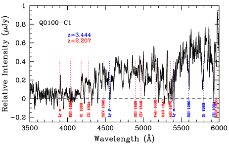
Figure 2.— Three examples of targets identified as spectroscopic blends of two redshifts within the 1-D extraction footprint of the primary target. Each panel has line identifications marked with colors corresponding to the two redshifts indicated (lower redshift in red, the higher redshift in blue). Since the lower-redshift features in the top 2 panels are sufficiently low that non-ionizing flux would contaminate the rest-frame LyC region of the higher redshift source, they were removed from the analysis sample. The bottom panel, which shows a spectroscopic blend of galaxies with $z=2.756$ and $z=2.822$, was retained in the sample but assigned the lower of the two redshifts.

3) A target was revealed to be a spectroscopic “blend” of unrelated objects, where the foreground object has the potential to cause a spurious (false-positive) detection of LyC flux if the source redshift is assumed to be the higher of the two redshifts. We identified 7 cases of spectroscopic blends, of which 5 were removed from the sample: Q0100-C1 ($z=3.44/2.21$; see Figure 2), Q0256-d4 ($z=3.67/2.63$; see Figure 2), Q0256-m11 ($z=3.090/2.09$), Q0256-md34 ($z=3.130/1.870$), and Q1009-C41 ($z=3.62/3.22/1.9$). The 5 discarded objects, had they been analyzed without the spectroscopic identification of the potential contamination, would all have been classified as LyC detections, with significance ranging from $3\sigma-7\sigma$ and flux level $f_{900}\simeq 0.050$ $\mu$Jy (m${}_{\rm AB}[LyC]\simeq 27.2$). In the remaining two cases, multiple redshifts were identified in the spectrum but the lower of the two redshifts was sufficiently high to allow a LyC measurement (i.e., $z\geq 2.75$): these are Q0933-M23 ($z=3.380/3.289$) and Q1549-D25 ($z=2.822/2.755$; see Figure 2). In both cases the target was retained in the sample, but the lower of the two redshifts was assigned for subsequent analysis.

Thus, in total, 13 of 136 galaxy targets were removed from the final KLCS sample. The 124 galaxies remaining in the final sample are listed (along with their coordinates, redshifts, and optical photometry) in Table 2.

Table 2The Keck Lyman Continuum Spectroscopic Sample

Name	RA	Dec	$z_{\rm sys}$	${\cal R}$	$G-{\cal R}$	$U_{n}-G$	$(G-{\cal R})_{0}$	$W_{\lambda}(\rm Ly\alpha)$	$f_{900}$	$\sigma_{900}$	$f_{1500}$	$\sigma_{1500}$	$(f_{900}/f_{1500})_{\rm obs}$
	(J2000)	(J2000)		(AB)	(AB)	(AB)	(AB)	(Å)	($\mu$Jy)	($\mu$Jy)	($\mu$Jy)	($\mu$Jy)
Q1422-c101	14:24:42.28	22:58:37.86	2.8767	24.17	0.85	3.79	0.73	-16.5	0.003	0.014	0.599	0.012	$0.005\pm 0.023$
Q1422-c49	14:24:36.11	22:52:41.34	3.1827	24.89	0.44	3.66	0.13	6.6	-0.004	0.013	0.327	0.014	$-0.012\pm 0.040$
Q1422-c63	14:24:30.18	22:53:56.21	3.0591	25.85	0.64	2.60	0.44	-0.1	-0.001	0.014	0.202	0.013	$-0.005\pm 0.069$
Q1422-c70	14:24:33.63	22:54:55.22	3.1286	25.45	0.92	2.72	0.68	6.3	0.005	0.014	0.248	0.013	$0.020\pm 0.056$
Q1422-c84	14:24:46.16	22:56:51.48	2.9754	24.70	0.88	3.21	0.69	-13.4	-0.001	0.012	0.383	0.015	$-0.003\pm 0.031$
Q1422-d42	14:24:27.72	22:53:50.71	3.1369	25.32	0.62	2.69	0.31	-10.5	0.053	0.014	0.373	0.012	$0.142\pm 0.038$
Q1422-d45	14:24:32.21	22:54:03.02	3.0717	24.11	0.31	2.49	0.11	0.3	0.000	0.014	0.953	0.014	$0.000\pm 0.015$
Q1422-d53	14:24:25.53	22:55:00.50	3.0864	24.23	0.83	2.57	0.59	-5.8	0.025	0.014	0.425	0.012	$0.059\pm 0.033$
Q1422-d57	14:24:43.25	22:56:06.68	2.9461	25.71	0.41	2.42	0.49	52.8	0.042	0.014	0.143	0.016	$0.294\pm 0.103$
Q1422-d68	14:24:32.94	22:58:29.13	3.2865	24.72	0.39	2.56	0.55	153.4	0.066	0.009	0.346	0.017	$0.191\pm 0.028$
Q1422-d78	14:24:40.49	22:59:35.30	3.1026	23.77	0.95	3.40	0.74	6.3	-0.008	0.011	0.655	0.012	$-0.012\pm 0.017$
Q1422-d81	14:24:31.45	22:59:51.57	3.1016	23.41	0.51	3.53	0.53	67.1	0.025	0.011	0.814	0.015	$0.031\pm 0.014$
Q1422-md119	14:24:36.18	22:55:40.31	2.7506	24.99	0.76	2.04	0.77	-5.0	0.025	0.025	0.298	0.012	$0.084\pm 0.084$
Q1422-md145	14:24:35.54	22:57:19.42	2.7998	24.89	0.95	2.09	0.99	13.4	-0.018	0.016	0.220	0.012	$-0.082\pm 0.073$
Q1422-md152	14:24:46.08	22:57:52.91	2.9407	24.06	1.18	2.20	1.04	-8.4	0.016	0.013	0.397	0.012	$0.040\pm 0.033$

Note. — Table 2 is published in its entirety in the machine-readable format. A portion is shown here for guidance regarding its form and content.

6. Measurements of Individual KLCS Spectra

6.1. Residual Interloper Contamination

As discussed in §1, foreground contamination leading to false-positive detection of LyC flux is a major concern for any putative detection of ionizing radiation from high redshift galaxies, and recent experience has shown that candidate LyC detections based on ground-based imaging surveys should be viewed with caution until additional observations – particularly multi-band HST imaging – can confirm the association of the detected flux with the known $z\sim 3$ galaxy or is more likely to be due to an unrelated object at a different (lower) redshift. In this section, we estimate the likelihood that our triage of the 1-D KLCS spectra has successfully identified most of the contaminated sources that would lead to false positive detections of LyC signal.

Recently, imaging surveys for LyC (Siana et al. 2007; Inoue & Iwata 2008; Nestor et al. 2011; Vanzella et al. 2012; Mostardi et al. 2013) have used Monte Carlo simulations based on the surface density of objects in a deep $U$ band images to estimate the probability that a random faint galaxy with (e.g.) $z<2.75$ would fall close enough to the centroid position of a targeted galaxy to cause a false-positive LyC detection. The probability of a chance superposition increases as the sensitivity limit for LyC detections becomes more sensitive; any galaxy with UV continuum surface brightness exceeding the typical statistical detection threshold over the bandpass used for LyC sensing is a potential source of contamination.

For the particular case of UV-color-selected LBGs at $z\sim 3$ – which require the presence of a photometric break between the observed $U_{\rm n}$ (3550/600) and $G$ (4730/1100) and a relatively blue color between $G$ and ${\cal R}$ (6830/1000) to have been selected for observation in the first place – the most likely sources of contamination are flat-spectrum (i.e., zero color on the AB magnitude system) galaxies with apparent magnitudes bright enough to yield a photometric or spectroscopic detection at $\lambda_{\rm obs}\simeq 3500$ Å, but faint enough that the resulting perturbation of the $U_{n}G{\cal R}$ photometry does not scatter the object out of the color selection window. The KLCS spectroscopically-observed sample has apparent $U_{n}\geq 26.13$, median $\langle U_{n}\rangle=27.7$, and typical spectroscopic detection limits in the LyC detection band (rest-wavelength range [880,910] Å) of $\sigma_{900}\simeq 0.01\mu$Jy ($10^{-31}$ ergs s^-1 cm^-2 Hz^-1, or $m_{\rm AB}[{\rm LyC}]=28.9$; see Figure 5 and Table 2.)

If we consider objects in the magnitude range $26<m_{\rm AB}(3500)<28.0$ as the most likely potential contaminants of the KLCS sample, we can use our deepest available UV images obtained under seeing conditions similar to those of the KLCS spectroscopic observations to estimate the probability of contamination of the KLCS slit apertures. The average surface density of detections in the range $26\leq m_{\rm AB}[3500]$Å $\leq 28$ is $\Sigma_{\rm avg}=88.7\pm 2.4$ arcmin^-2, where the uncertainty represents the scatter in $\Sigma_{\rm avg}$ among the 4 fields. Each KLCS spectroscopic extraction aperture subtends 1${}^{\prime\prime}\mskip-7.6mu.\,$2 by 1${}^{\prime\prime}\mskip-7.6mu.\,$35, or a solid angle of 1.6 arcsec² ($4.4\times 10^{-4}$ arcmin^-2). The probability that the centroid of a $m_{\rm AB}=26-28$ object (at any redshift) falls within the extraction aperture for any single KLCS target is $P\simeq 88.7\times 4.4\times 10^{-4}=0.039$; thus, in a sample of 128, we expect $N_{c}\sim 128\times 0.039\simeq 5$ will be affected by such contamination.

While this type of argument cannot exclude the possibility that there remain unidentified false-positive detections in the KLCS sample, the fact that the number of slit apertures predicted to be affected by chance superposition of UV-faint foreground galaxies is similar to the number of spectra identified as blends with foreground galaxies suggests that our spectroscopic “triage” has likely removed most of the contaminants that would lead to false positive LyC detections.

6.2. Galaxy Systemic Redshifts

Because our primary goal is to measure the residual flux averaged over a relatively broad window in rest-wavelength, precise systemic redshift measurements are not critical. However, since we will be combining individual spectra into composite stacks (§8), we assigned our best estimate of $z_{\rm s}$ for each galaxy based on the information in hand. Of the 124 sources in the KLCS analysis sample, 55 (44%) have measurements of nebular [O III] emission lines in the rest-frame optical obtained using Keck/MOSFIRE (McLean et al. 2012; Steidel et al. 2014.) In all such cases, the measured $z_{\rm neb}$ is assumed to define the systemic redshift $z_{\rm sys}$, with an uncertainty of $\simeq 15-20$ km s${}^{-1}\,$.

For objects lacking nebular emission line measurements, we used estimates of $z_{\rm sys}$ based on the full KBSS-MOSFIRE sample (Steidel et al. 2014; Strom et al. 2017) with $z>2.0$ and existing high-quality rest-UV spectra. These were used to calibrate relationships between $z_{\rm sys}$ and redshifts measured from features in the rest-frame FUV spectra, strong interstellar absorption lines ($z_{\rm IS}$) and/or the centroid of Lyman-$\alpha$ emission ($z_{\rm Ly\alpha}$). As for previous estimates of this kind (e.g., Adelberger et al. 2003; Steidel et al. 2010; Rudie et al. 2012), we adopt rules that depend on the particular combination of features available in each spectrum, where spectra fall into one of 3 categories: (a) those with measurements of both $z_{\rm Ly\alpha}$ and $z_{\rm IS}$; (b) those with $z_{\rm IS}$ but without $z_{\rm Ly\alpha}$ (generally because the $\rm Ly\alpha$ feature appears in absorption); and (c) those with only $z_{\rm Ly\alpha}$ available.

Figure 3.— Residuals in the UV-based estimates of $z_{\rm sys}$ (using equations 3-5) (black points) relative to the nebular redshifts for the 55 KLCS galaxies with both UV and nebular redshifts. The measurements of $z_{\rm Ly\alpha}$ and $z_{\rm IS}$ for individual galaxies are represented by open red triangles and open blue squares, respectively. The mean residual velocity offset $\langle\Delta v_{\rm uv}\rangle=-1\pm 14$ km s${}^{-1}\,$, with rms$=104$ km s${}^{-1}\,$.

For galaxies in category (a), comprising $\simeq 60$% of the KLCS sample,

$$z_{\rm sys}=z_{\rm IS}+0.40(z_{\rm Ly\alpha}-z_{\rm IS})~{};$$ (3)

for category (b) ($\simeq 30$% of the KLCS sample) :

$$z_{\rm sys}=z_{\rm IS}+\frac{\Delta v_{\rm IS}}{c}(1+z_{\rm IS}),$$ (4)

with $\rm\Delta v_{IS}\ =130$ km s${}^{-1}\,$  ; for category (c) ($\simeq 10$% of the KLCS sample):

$$z_{\rm sys}=z_{\rm Ly\alpha}-\frac{\rm\Delta v_{\rm Ly\alpha}}{c}(1+z_{\rm Ly\alpha})~{};$$ (5)

with $\rm\Delta v_{\rm Ly\alpha}=235$ km s${}^{-1}\,$. The residual velocity offset and rms errors after applying these rules to the UV spectra of the 55 galaxies with measurements of $z_{\rm neb}$ (Figure 3) is

$$\langle c(z_{\rm sys,uv}-z_{\rm neb})/(1+z_{\rm neb})\rangle=-1\pm 104~{}\rm km~{}s^{-1}\,,$$ (6)

where the quantity inside the angle brackets is equivalent to $\Delta v_{\rm UV}$ in Figure 3.

The best available value of $z_{\rm sys}$ is given for each galaxy in Table 2.

6.3. LyC Measurements

All quantitative measurements or limits on the flux density of residual LyC emission have been evaluated over a fixed bandpass in the source rest frame, placed just shortward of the Lyman limit:

$$f_{900}\equiv\langle f_{\nu}(\lambda_{0})\rangle\quad;\quad 880\leq\lambda_{0}/{\textrm{\AA}}\leq 910~{}.$$ (7)

We also define a rest-frame bandpass to represent the FUV non-ionizing flux density,

$$f_{1500}\equiv\langle f_{\nu}(\lambda_{0})\rangle\quad;\quad 1475\leq\lambda_{0}/{\textrm{\AA}}\leq 1525~{}.$$ (8)

The choice of the interval [880,910] for the LyC measurement is a compromise based on two considerations. First, ideally the LyC measurement should be made as close as possible to the rest-frame Lyman limit of the galaxy, and integrated over the smallest wavelength range feasible given the noise level of the spectra, in order to minimize the effects of H I in the IGM along the line of sight. As discussed in detail in §7, the opacity of the IGM to LyC photons is the largest source of uncertainty in the measurement of the emergent ionizing photon flux from a galaxy. The mean free path of H-ionizing photons emitted at $\langle z_{\rm s}\rangle=3.05$ corresponds to a redshift interval of $\Delta z\sim 0.25$ (e.g., Rudie et al. 2013), or to $\sim 60$ Å in the rest frame; i.e., the flux density at $\lambda_{0}\simeq 850$ Å is reduced by an average factor of e ($\sim 2.72$) relative to its emergent value. By using the [880,910] interval, to a first approximation the average IGM LyC optical depth due to intervening material is $\langle\tau_{\rm igm}\rangle\lower 2.15277pt\hbox{$\;\buildrel<\over{\sim}\;$}0.5$.

An additional consideration is the wavelength range over which the Keck/LRIS-B system sensitivity remains high. Although the UV sensitivity of Keck/LRIS-B is the highest among instruments of its kind (Steidel et al. 2004), it decreases with wavelength shortward of 3500 Å, particularly when atmospheric opacity is included. The lowest redshift source included in KLCS has $z_{\rm s}=2.718$ (Q0100-MD6), placing $\lambda_{0}=880$ Å at an observed wavelength of 3272 Å , where the LRIS-B end-to-end throughput with the d500 beamsplitter has dropped to $\simeq 20$% from $\lower 2.15277pt\hbox{$\;\buildrel>\over{\sim}\;$}50$% near 4000 Å. Including the atmosphere, these numbers reduce to $\sim 11$% and $\sim 40$% at a typical airmass of 1.10 on Mauna Kea. At the mean redshift of the KLCS sample ($\langle z_{\rm s}\rangle=3.05$), [880,910] corresponds to an observed-frame interval [3560,3690] Å, where the instrumental throughput averages $\simeq 35$%.

Thus, [880,910] is observable over the full range of KLCS, and is narrow enough to minimize the IGM opacity against which escaping flux must be detected, but sufficiently broad to allow for improved photon statistics while reducing the fluctuations due to discrete H I absorption lines arising from intervening material, superposed on the rest-frame LyC.

Figure 4 presents the measured values of $f_{900}$, with objects grouped and ordered according to slitmask and the relative physical position on the mask (along the slit direction) for each target. Targets having $>3\sigma$ detections of $f_{900}$ are labeled. The values of $f_{900}$ and their associated statistical error ($\sigma_{900}$) for KLCS galaxies are listed in Table 2. Also given in Table 2 are measurements of the non-ionizing UV continuum flux density $f_{1500}$ (equation 8) measured directly from the individual 1-D flux-calibrated spectra.

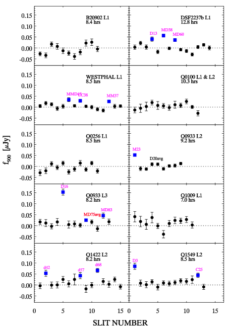
Figure 4.— Measurements of the average flux density in the rest-frame interval [880,910] Å ($f_{900}$) for the 124 LBGs (circles) in the KLCS analysis sample. Each slit mask used has its own panel, with the order of objects following their relative physical placement on the slitmask. The total exposure time in hours for each mask is indicated under the mask name. The errors shown are $\pm 1\sigma$ statistical errors derived accounting for counting statistics and detector noise. A total of 15 out of 124 galaxies are nominal detections, with $f_{900}>3\sigma_{900}$; these are marked with square (blue) symbols. Note that galaxies Q0933-MD75 and Q0933-D20 were observed twice, on masks q0933_L2 and q0933_L3– points labeled in red represent the weighted average measurement from the two independent spectra.

The measurements and uncertainties for $f_{900}$ and $f_{1500}$ [and their ratio ($f_{900}/f_{1500})_{\rm obs}$] were obtained directly from the 1-D spectra and associated error arrays based on the noise model described in §A.5.1; we have made no attempt to apply aperture corrections to the spectroscopic flux density measurements (the photometric measurements in the $U_{\rm n}G{\cal R}$ system are also provided in Table 2) but we believe that the relative spectrophotometry of the 1D spectra has systematic errors $\lower 2.15277pt\hbox{$\;\buildrel<\over{\sim}\;$}5$%; uncertainties in the calibration of LRIS-R relative to LRIS-B spectra may contribute additional $\lower 2.15277pt\hbox{$\;\buildrel<\over{\sim}\;$}10\%$ systematic uncertainty in $(f_{900}/f_{1500})_{\rm obs}$.

The flux error-bars in Figure 4 are statistical errors based on the noise model presented in §A.5.1, with typical values of $\sigma_{900}=0.01$ $\mu$Jy; most objects on each mask have $f_{900}$ measurements consistent with zero to within 1-2$\sigma_{900}$.

Grouping observations by slit-mask allows us to monitor the presence of systematic errors from mask to mask. It is also a useful way to inspect the data for correlations with object position on a given slit-mask. It is apparent from Figure 4 that mask B20902-L1 (and possibly others) has residual systematic errors manifesting as correlated behavior of $f_{900}$ as a function of position on the slitmask. Although the maximum deviation from zero in the b20902_L1 panel is only $\sim 2\sigma_{900}$, there appear to be systematic undulations relative to zero with amplitude comparable to the random errors. The systematics appear to have larger excursions to $f_{900}<0$, as might occur from over-subtraction of the background due to contamination of slit regions used to model it by either scattered light (judged to be the dominant factor for mask b20902_L1), or by contributions from unmasked sources falling along the slit.

Systematic over-subtraction of the background level was also noted for the sample of 14 sources presented by Shapley et al. (2006) (S06) – these authors found that the measured $f_{900}$ for objects without significant detections was centered around an unphysical negative value (see their Figure 5). As discussed in detail in §4.2 (see also Appendix A.6), considerable effort was invested in improving the flat fielding (with its tendency to exacerbate problems with non-uniform scattered light (§A.1) and 2-D background subtraction. The tests summarized in appendix A.6 suggest that these were generally successful. We show below that the procedures have also reduced the residual systematic errors in extracted 1-D spectra to a level significantly smaller than the random errors.

Table 3Objects with Individual LyC Detections

Object	$z_{\rm sys}$	($L/L^{\ast}$)	$(f_{900}/f_{1500})_{\rm obs}$
Q0933-D16	3.0468	0.51	$0.54\pm 0.06$
Q0933-M23	3.2890	0.92	$0.26\pm 0.03$
Q0933-MD75	2.9131	0.89	$0.10\pm 0.02$
Q0933-MD83	2.8790	0.60	$0.15\pm 0.04$
Westphal-CC38	3.0729	1.00	$0.06\pm 0.01$
Westphal-MM37	3.4215	1.23	$0.05\pm 0.01$
Westphal-MMD45	2.9366	1.42	$0.09\pm 0.02$
Q1422-d42	3.1369	0.47	$0.14\pm 0.04$
Q1422-d57	2.9461	0.30	$0.30\pm 0.10$
Q1422-d68	3.2865	0.88	$0.19\pm 0.03$
Q1549-C25	3.1526	0.74	$0.08\pm 0.02$
Q1549-D3	2.9373	1.16	$0.06\pm 0.01$
DSF2237b-D13	2.9212	0.58	$0.08\pm 0.02$
DSF2237b-MD38	3.3278	1.47	$0.07\pm 0.01$
DSF2237b-MD60	3.1413	0.67	$0.09\pm 0.02$

To verify that this is the case, we excluded all galaxy measurements for which $|f_{900}|>3\sigma_{900}$ where $\sigma_{900}$ is the statistical error estimate. For the remaining sample of 106 measurements, $\langle f_{900}/\sigma_{900}\rangle=0.31\pm 1.33$, with median $f_{900}/\sigma_{900}=0.44$, and inter-quartile range [-0.50,+1.41]. Excluding the two masks (B20902-L1 and Q1009-L1) with the most obvious systematic issues, the results remain largely unchanged: $\langle f_{900}/\sigma_{900}\rangle=0.28\pm 1.32$, with median $0.44$ and inter-quartile range [-0.66,+1.25]. Under the null hypothesis that $f_{900}=0$ and that systematic errors are small compared to normally distributed random errors, one expects $\langle f_{900}/\sigma_{900}\rangle=0.0\pm 1.0$. As we shall see, the true values of $f_{900}$ are likely greater than zero for some fraction of the sample with $|f_{900}/\sigma_{900}|<3$; since the standard deviation of $f_{900}/\sigma_{900}$ is only $\sim 30$% larger than expected under the null hypothesis, we believe that residual systematic errors in $f_{900}$ are sub-dominant compared to statistical errors. In the remainder of the analysis below, we continue to assume that our model for random errors in the spectra (§A.5.1) accurately describes the uncertainties.

Figure 5.— Statistical uncertainties in the measurements of $f_{900}$, in units of $\mu$Jy, for all galaxies in the KLCS final sample. The yellow circles and blue triangles represent formally detected and formally undetected objects, respectively.

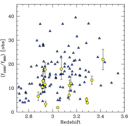
Figure 6.— Lower limits ($3\sigma$) on $(f_{1500}/f_{900})_{\rm obs}$ for objects without LyC detections (blue triangles). Objects with formal LyC detections are shown as yellow points with $1\sigma$ error bars.

Thus, 15 of 124 galaxies have $f_{900}>3\sigma_{900}$, which henceforth are referred to as “detected”; their properties are listed individually in Table 3. The same objects are marked using blue squares in Figure 4. Note that one of the objects in Table 3, Q1549-C25 [$(f_{900}/f_{1500})_{\rm obs}=0.08$], has been discussed in detail by Shapley et al. (2016); in addition to the LyC flux measurement, it has also been observed with multi-band HST imaging (see Mostardi et al. 2015) which indicates no evidence for a contaminating foreground source that might have caused a false-positive LyC detection. The only other confirmed LyC detection of a $z\sim 3$ galaxy is “Ion-2” ($z_{\rm s}=3.22$), which has $(f_{900}/f_{1500})_{\rm obs}\simeq 0.13$ and rest-frame UV luminosity $\sim L_{\rm uv}^{\ast}$ (Vanzella et al. 2015; de Barros et al. 2016). Most of the objects in Table 3 have $(f_{900}/f_{1500})_{\rm obs}$ similar to the two confirmed LyC detections.

Figure 5 shows all 124 KLCS targets on a plot of $\sigma_{900}$ versus redshift. Note that $\sigma_{900}$ shows a trend of increasing toward lower redshift; this is due to the decreasing instrumental sensitivity at rest-frame wavelengths [880,910] Å  which (as we have seen) changes by a factor of a few over the range $2.75\lower 2.15277pt\hbox{$\;\buildrel<\over{\sim}\;$}z\lower 2.15277pt\hbox{$\;\buildrel<\over{\sim}\;$}3.4$ (where [880,910] falls at observed wavelengths $3300\lower 2.15277pt\hbox{$\;\buildrel<\over{\sim}\;$}(\lambda/\textrm{\AA})\lower 2.15277pt\hbox{$\;\buildrel<\over{\sim}\;$}4000$.)

Figure 6 shows a combination of formal detections and – for the non-detections – the adopted 3$\sigma$ lower limits on the ratio $(f_{1500}/f_{900})_{\rm obs}$ using the measurements and uncertainties given in Table 2. Note that the formally detected objects lie well within the distribution of $3\sigma$ upper limits of the non-detections. The implications of these results for the distribution of LyC flux within the observed sample requires a quantitative assessment of the extent to which H I gas outside of galaxies (but along the line of sight) has censored our ability to detect LyC flux when it is present; we address this issue in §7.

6.4. LyC Detection vs. Other Galaxy Properties

In this section we briefly review the properties of galaxies with individual LyC detections versus the majority that do not have individual detections. We argue below (§8) that unambiguous interpretation of LyC detection statistics requires the use of ensembles of galaxies.

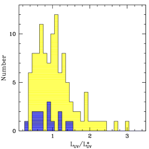
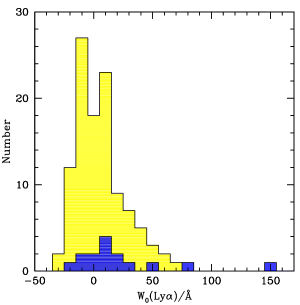
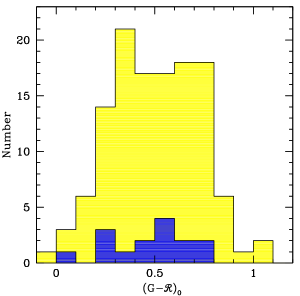
Figure 7.— (Left:) Distribution of rest-frame UV luminosity relative to $L^{\ast}_{UV}$ at $z\simeq 3$ for galaxies with individually detected $f_{900}$ (dark/blue) compared to that of the sample with $f_{900}<3\sigma_{900}$ (light/yellow). (Center:) As for the lefthand panel, comparing the distribution of rest-frame equivalent width of $\rm Ly\alpha$, $W_{\lambda}(\rm Ly\alpha)$. (Right:) As for the lefthand panel, comparing the distribution of rest-UV continuum color (see §6.4). 2-sample Kolmogorov-Smirnov (KS) tests applied to all 3 cases cannot significantly reject the null hypothesis that the distributions of formally detected and formally undetected objects are drawn from the same parent population.

Figure 7 compares the distributions in 3 empirical galaxy properties for the LyC-detected and LyC-undetected sub-samples of KLCS (with 15 and 109 objects, respectively.) The left-most panel of Fig. 7 shows the rest-UV luminosity distribution, relative to $L_{\rm uv}^{\ast}$ in the far-UV (rest-frame 1700 Å) luminosity function at $z\sim 3$ (Reddy & Steidel 2009). As discussed in §5 above, most KLCS galaxies have $L_{\rm uv}$ within a factor of a few of $L_{\rm UV}^{\ast}$. The sub-sample with formal LyC detections occupies a slightly narrower range of luminosity, though a two-sample KS test shows that the two luminosity distributions are statistically consistent with being drawn from the same parent population.

As one of the most easily-observed and measured spectroscopic characteristics of high redshift star-forming galaxies, the rest-frame equivalent width of the Lyman-$\alpha$ emission line, $W_{\lambda}(\rm Ly\alpha)$, is a useful diagnostic, and has been shown to correlate strongly with other more subtle spectroscopic features present in the spectra of LBGs (Shapley et al. 2003; Kornei et al. 2010). We measured $W_{\lambda}(\rm Ly\alpha)$ for the KLCS galaxy sample following the method described in Kornei et al. (2010); the values are listed in Table 2. The center panel of Figure 7 (see also Table 2) shows the distribution of $W_{\lambda}(\rm Ly\alpha)$ for the full KLCS galaxy sample, divided according to whether or not they are formally detected in the LyC band [880,910]. Although the detected sub-sample tends to have $\rm Ly\alpha$ in emission, and the fraction of objects with LyC detected appears to be correlated with $\rm Ly\alpha$ equivalent width, a two-sample KS test cannot reject the null hypothesis that the sub-samples are drawn from the same parent population.

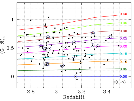
Figure 8.— UV color vs. redshift for the KLCS galaxy sample, where the $(G-{\cal R})_{0}$ is the observed $G-{\cal R}$ after correcting for the contribution of $\rm Ly\alpha$ emission or absorption to the $G$ band, based on each object’s spectrum, and accounting for the average line blanketing of the $G$ band by the IGM+CGM (see §7). The color-coded curves are the expected track for the BPASSv2.1-300bin-Z001 SPS model (§9.2) after applying reddening according to the Reddy et al. (2016a) attenuation relation with the indicated value of $E(B-V)$. The 15 galaxies with $>3\sigma$ LyC detections are indicated with larger open circles. CGM+IGM .

As described in more detail elsewhere (Shapley et al. 2003; Steidel et al. 2003; Reddy & Steidel 2009) the $z\sim 3$ LBG $U_{\rm n}G{\cal R}$ color selection imposes small systematic differences in the redshift selection function depending on the intrinsic galaxy properties, in the sense that intrinsically redder galaxies are less likely to satisfy the selection criteria at the high redshift end of the selection window. The main reason for this is increased line blanketing from the $\rm Ly\alpha$ forest with redshift. Galaxies with very strong $\rm Ly\alpha$ features (in either emission or absorption) affect the observed $G-{\cal R}$ color for similar reasons, since $\rm Ly\alpha$ falls in the observed $G$ band throughout the KLCS redshift range. However, since the full KLCS sample has spectroscopic measurements, we can correct the observed $G-{\cal R}$ color of individual galaxies for both effects, thereby yielding estimates of the intrinsic UV continuum color. Figure 8 shows the measurements for individual KLCS galaxies as a function of redshift in terms of $(G-{\cal R})_{0}$, the proxy for continuum color after correction for the mean IGM absorption in the $G$ band and the individual $W_{\lambda}(\rm Ly\alpha)$ . The KLCS galaxies with individual $>3\sigma$ LyC detections are circled, and their distribution is compared with the full sample in the rightmost panel of Figure 7.

As for $L_{\rm uv}$ and $W_{\lambda}(\rm Ly\alpha)$, the sub-sample having direct individual detections is consistent with being drawn from the same distribution in $(G-{\cal R})_{0}$ as the full KLCS sample. We discuss the statistical connections between LyC leakage and galaxy properties in more detail in §8.

7. The Opacity of the Intergalactic Medium

The opacity of the IGM has been reasonably well-quantified in a statistical sense (e.g., Madau 1995; Faucher-Giguère et al. 2008; Prochaska et al. 2009; Rudie et al. 2013; Inoue et al. 2014) from high resolution spectroscopic surveys of relatively bright QSOs. Modeling the statistics of IGM absorption is essential for understanding the implications of any survey seeking to quantify the intensity of ionizing photons escaping from high redshift galaxies. In order to convert our observations of $(f_{900}/f_{1500})_{\rm obs}$ into the more relevant spectrum of emergent ionizing radiation from galaxies, we used a set of IGM attenuation models using a Monte Carlo technique described by Nestor et al. (2011) (see also Bershady et al. 1999; Shapley et al. 2006; Inoue & Iwata 2008; Inoue et al. 2014 for similar models), with H I distribution function ($f(N_{\rm HI},X)$) parameters updated based on the KBSS QSO sightlines, including the effects of the CGM (Rudie et al. 2013.) The models produce full realizations of individual IGM sightlines toward a source with redshift $z_{\rm s}$ by drawing from the empirically-calibrated incidence of intervening H I as a function of $N_{\rm HI}$ and redshift, over the range $12\leq({\rm log~{}(N_{\rm HI}/cm^{-2}})\leq 22.0$ and $1.6\leq z\leq z_{\rm s}$, the details of which are presented in Appendix B. Each simulated spectrum includes both line blanketing from Lyman series absorption lines (most relevant for the low-$N_{\rm HI}$ systems) and LyC opacity (dominated by systems having log $N_{\rm HI}$ $\simeq 16-18$) as a function of observed wavelength over the range $3100\leq\lambda_{\rm obs}\leq 1216(1+z_{\rm s})$. By creating an ensemble of simulations with the same redshift distribution as the sources in the observed KLCS sample, one can make precise statistical statements about the effect of the IGM on the measurements of $f_{\rm 900}$.

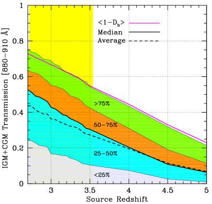
Figure 9.— Illustration of the predicted IGM+CGM transmission evaluated at rest-frame [880,910] Å as a function of source redshift. The colored bands indicate percentile ranges (see Table 12), the dashed black curve is the mean transmission, and the magenta solid curve is $\langle 1-D_{\rm B}\rangle$, the mean transmission between Ly$\beta$ and the Lyman limit in the rest frame of the source (see discussion in AppendixB). The KLCS redshift range is (lightly) shaded with a rectangular box.

Monte Carlo simulations were run for two separate models based on the parametrization of $f(N_{\rm HI},X)$ (Figure 31.) The first, which we call “IGM-Only”, assumes that every sightline to a KLCS source is equivalent to randomly selecting H I absorbers from the distribution function in a way that depends only on redshift and $N_{\rm HI}$, i.e. the “Average IGM” parametrization in Figure 31. Rudie et al. (2012) showed that regions within 300 kpc (physical) of galaxies at $z\sim 2.4$ give rise to a significantly higher incidence of ${\rm log}N_{\rm HI}\lower 2.15277pt\hbox{$\;\buildrel>\over{\sim}\;$}14$ absorption. To account for this, a second set of realizations, called “IGM+CGM”, includes a model for regions of enhanced H I absorption arising in the circum-galactic medium (CGM) near the source galaxies. As discussed in Appendix B, the CGM H I absorber frequency distribution function $f(N_{\rm HI},X)[\rm CGM]$ (Figure 31) is based on the KBSS survey results (Rudie et al. 2012, 2013) detailing the distribution of $N_{\rm HI}$ along sightlines passing within 50-300 physical kpc (pkpc) and within 700 km s${}^{-1}\,$in redshift (i.e., $\left|{\Delta z}\right|\leq 0.0023(1+z_{\rm s})$ of spectroscopically identified galaxies with $2.0\lower 2.15277pt\hbox{$\;\buildrel<\over{\sim}\;$}z\lower 2.15277pt\hbox{$\;\buildrel<\over{\sim}\;$}2.8$. For modeling lines of sight in the “IGM+CGM” simulations we used the CGM parameters for $f(N_{\rm HI},X)$ (Table 11) for redshifts $z_{\rm s}-\Delta z\leq z\leq z_{\rm s}$ and the “Average IGM” formulation $z<(z_{\rm s}-\Delta z$), where $\Delta z=0.0023(1+z_{\rm s})$ ($c\Delta z=700$ km s${}^{-1}\,$.) For most purposes in this paper, the “IGM+CGM” is the more relevant of the two; results from both are included in Table 12. The differences between “IGM+CGM” and “IGM-only” opacity model are discussed below.

Since we have adopted [880,910] Å in the rest frame of the source as our LyC measurement band, of greatest interest is the prediction for the statistical reduction by the CGM+IGM of the flux density at observed wavelengths $880(1+z_{\rm s})\leq\lambda_{\rm obs}\leq 910(1+z_{\rm s}$). We define

$$\langle t_{900}\rangle \equiv \langle{\rm exp}(-\tau(\lambda_{\rm obs})\rangle,$$ (9)

$$880(1+z_{\rm s}) \leq (\lambda_{\rm obs}/{\textrm{\AA}})\leq 910(1+z_{\rm s}).$$ (10)

With this definition of $t_{900}$, we can correct observed values of $\langle f_{900}/f_{1500}\rangle_{\rm obs}$ for IGM(+CGM) attenuation

$$\langle f_{900}/f_{1500}\rangle_{\rm out}=\langle f_{900}/f_{1500}\rangle_{\rm obs}/\langle t_{900}\rangle,$$ (11)

where $\langle f_{900}/f_{1500}\rangle_{\rm out}$ is the emergent flux density ratio that would be measured by an observer at $z=0$ if there were no opacity contribution from the CGM and IGM along the line of sight; as discussed in more detail below (§10, §11.4), $\langle f_{900}/f_{1500}\rangle_{\rm out}$ is the quantity relevant to calculations of ionizing emissivity of galaxy populations.

Figure 9 illustrates how the distributions of “IGM-Only” and “IGM+CGM” transmission $t_{900}$ depend on $z_{\rm s}$, with the range selected for KLCS shaded yellow. Table 12 summarizes the results of the IGM modeling in terms of the percentiles (10, 25, 50, 75, and 90th) of the IGM or IGM+CGM transmission at particular rest wavelength intervals of interest, all as a function of source redshift. Source redshift values were modeled using small ($\Delta z=0.05$) increments over the KLCS redshift range, but we have also included values for sources with $z_{s}>3.5$ to provide some intuition about the rapid decline in IGM transmission as redshift increases.

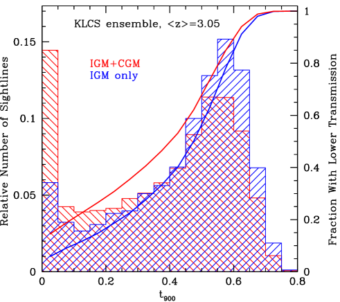
Figure 10.— Histogram of the probability density function of $t_{900}$, the net transmission in the rest wavelength interval [880,910] for sources having identical $z_{\rm s}$ distribution as the KLCS ensemble. The histograms show the average of 1000 sets of 124 sightlines: blue-hatched includes only IGM opacity while the red-hatched includes IGM+CGM opacity. The continuous curves, color coded in the same way, show the cumulative fraction of sightlines with lower $t_{900}$ (both curves refer to the righthand axis). Note that the main effect of including the CGM is to flatten the distribution for $t_{900}\lower 2.15277pt\hbox{$\;\buildrel>\over{\sim}\;$}0.05$ while increasing the expected number of opaque sightlines ($t_{900}<0.05$) by a factor of $\simeq 3$ and decreasing the relative number of sightlines with the highest $t_{900}$.

Even within the redshift range spanned by the KLCS sample, $\langle t_{900}\rangle$ varies by almost a factor of 2; however, if we treat the KLCS sample as an ensemble of 124 sightlines with $2.75\lower 2.15277pt\hbox{$\;\buildrel<\over{\sim}\;$}z_{\rm s}\leq 3.55$, the IGM+CGM simulations predict that the ensemble average $\langle t_{900}\rangle=0.371$ with 68% confidence interval $t_{68}=[0.353,0.392]$, i.e. an uncertainty of $\sim 5$% on $\langle t_{900}\rangle$ for the ensemble. Fig. 10 shows the full distribution of $t_{900}$ expected for ensembles of 124 sightlines with the same redshift distribution as KLCS, for both the IGM Only and IGM+CGM opacity models.

One can see from Figure 10 that there are two main effects of including the opacity of the CGM: (1) it increases by a factor of $\sim 3$ the number of sightlines with very low transmission ($t_{900}<0.05$); and (2) it significantly decreases the fraction of sightlines expected to have transmission near the maximum of $t_{900}\simeq 0.6$. The latter would be (all other factors being equal) the most likely to yield detectable LyC signal in the spectra of individual galaxies. This point illustrates the importance of accounting statistically for LyC attenuation by gas which is outside of the galaxies, but near enough to be observationally indistinguishable from a case of zero LyC photon escape from the galaxy ISM.

For some purposes (see §8), it is useful to form ensemble average transmission spectra covering a wider range in rest-wavelength than we have used to measure $t_{900}$. Figure 11 illustrates the rest-wavelength dependence of ensemble average transmission spectra for $z_{\rm s}=3.05$. These spectra were created from an ensemble of 10000 realizations of the full transmission spectra predicted by the Monte Carlo IGM+CGM model, sorting them by $t_{900}$, and averaging in percentile bins.

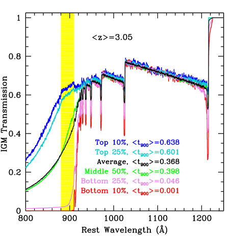
Figure 11.— Transmission spectra, in the rest frame of the source, for $\langle z\rangle=3.05$ for an ensemble of 10000 lines of sight assuming the CGM+IGM opacity model. The various color-coded spectra represent averages within percentile ranges of $t_{900}$. Note that the variations in line blanketing from the Ly$\alpha$ forest are small for $\lambda_{0}>940$ Å (except where affected by the CGM, which manifest here as small regions of enhanced absorption near the rest-frame wavelengths of each Lyman series line). The variations are large in the region of primary interest ([880,910] Å, shaded yellow) because the effective opacity is dominated by much rarer absorption systems with high $N_{\rm HI}$ (see Appendix B.)

Fig. 11 shows that for $\lower 2.15277pt\hbox{$\;\buildrel>\over{\sim}\;$}10$% of sightlines at $z_{s}=3.05$ (“Top 10%” spectrum in the figure) there will be little or no attenuation over and above that produced by line blanketing. However, given typical detection limits for LyC flux, at least the “Bottom 25%” shown in Figure 11 will appear be be optically thick to their own LyC radiation, due entirely to attenuation by intervening H I at $D>50$ kpc arising due to the opacity of the combined CGM+IGM.

7.1. IGM Transmission: Sampling Issues

Table 4Sampling Statistics for LyC Transmission (CGM+IGM)

$z_{\rm s}$	$\langle t_{900}\rangle$	$t_{68}$	$\delta t_{900}/\langle t_{900}\rangle$
			$N=15$	$N=30$	$N=60$	$N=120$
2.75	0.453	[0.093-0.670]	0.141	0.101	0.067	0.048
3.00	0.391	[0.074-0.607]	0.153	0.108	0.073	0.052
3.25	0.325	[0.018-0.540]	0.173	0.120	0.082	0.056
3.50	0.271	[0.013-0.467]	0.184	0.128	0.088	0.063

Assuming the “IGM+CGM” opacity model, at $z\sim 3$, the 68% confidence interval for a single realization of $t_{900}$ at $z_{\rm s}\simeq 3.05$ is $t_{\rm 900}=[0.038,0.589]$; the corresponding 68% confidence intervals are $t_{900}=[0.076,0.665]$ at $z_{\rm s}=2.70$ , and $t_{900}=[0.017,0.471]$ at $z=3.50$. The implications of these broad distributions are worth stating explicitly: the LyC-detectability of a galaxy with a given intrinsic (i.e., emergent) $(f_{900}/f_{1500})_{\rm out}$ is to a great extent controlled by the statistics of the IGM transmission, which is uncertain by factors of between 5 and 10 even over the limited redshift range $2.70\lower 2.15277pt\hbox{$\;\buildrel<\over{\sim}\;$}z_{\rm s}\lower 2.15277pt\hbox{$\;\buildrel<\over{\sim}\;$}3.50$. Conversely, a single measurement of $(f_{900}/f_{1500})_{\rm obs}$ cannot be converted into an intrinsic property of the source, for the same reason (see, e.g., Vanzella et al. 2015; Shapley et al. 2016.)

However, $\langle t_{900}(z_{\rm s})\rangle$, the mean transmissivity of the IGM for a source at $z=z_{\rm s}$, and its uncertainty $\delta t_{900}(z_{\rm s},N)$ can be quantified for an ensemble of $N$ sightlines using the Monte Carlo models described in Appendix B. For example, assuming $z_{\rm s}=3.0$, the number of independent IGM sightlines one must sample in order to reduce $\delta t_{900}(3.0,N)$ to less than 10 (5) percent of $\langle t_{900}(3.0)\rangle$ is $N=36$ (150). In other words, if the spectra of 36 sources at $z_{\rm s}=3.0$ are averaged to produce a measurement of $\langle f_{900}/f_{1500}\rangle_{\rm obs}$, then $\langle(f_{900}/f_{1500})_{\rm out}\rangle=\langle(f_{900}/f_{1500})_{\rm obs}\rangle/(t_{900}\pm\delta t_{900})$, and the IGM correction contributes a fractional uncertainty to the inferred emergent flux density ratio of $\simeq 10$%. Some example statistics relevant for the KLCS redshift range and sample size are given in Table 4.

This type of analysis is useful when one has observations of a particular class of object (grouped by known property, e.g. $L_{\rm uv}$, $z_{\rm s}$, $W_{\lambda}(\rm Ly\alpha)$, inferred extinction) forming a subset of the full sample: as long as the subset has sufficiently large $N$, the statistical knowledge of the IGM opacity can be used to derive the average intrinsic LyC properties of that class. The validity of this procedure depends on (1) the assumption that each line of sight in the sample is uncorrelated with any other line of sight in the same ensemble and (2) that the IGM+CGM opacity model is an accurate statistical description of the true opacity.

The first assumption – that lines of sight are independent – is almost certainly not valid when a survey is conducted in a single contiguous field of angular size $\sim 10$${}^{\prime}~{}$(transverse scale of $\sim 5$ pMpc at $z\sim 3$), as has often been the case for reasons of practicality (e.g., Shapley et al. 2006; Nestor et al. 2011; Mostardi et al. 2013, 2015; Vanzella et al. 2010; Siana et al. 2015). Correlated sightlines could be especially problematic in fields known to contain significant galaxy over-densities at or just below the source redshifts. As has been discussed by (e.g.) Shapley et al. (2006): if observed sources are located in regions containing more (or less) gas near $N_{\rm HI}$$=10^{17}$ cm^-2 than average, their “local” IGM could skew significantly away from expectations if an “average” line of sight is assumed. The effect is likely to be negligible for $\rm Ly\alpha$ forest blanketing, but could strongly influence $f_{900}$, since it relies on the statistics of small numbers through the incidence of relatively high column density H I over a small redshift path ($\Delta z\simeq 0.14$ for $z_{s}=3.05$ for our LyC region [880,910] Å.)

The full KLCS sample is relatively insensitive to the effects of correlations between IGM sightlines by virtue of the fact that it is comprises 9 independent survey regions. Similarly, the IGM opacity model is based on the statistics of 15 independent QSO sightlines in the KBSS survey (Rudie et al. 2013), and the CGM corrections to the IGM model are based on regions near galaxies selected using essentially identical criteria to those used for KLCS (albeit at slightly lower redshift; see Rudie et al. 2013).

Nevertheless, it is worth pointing out caveats associated with the CGM+IGM opacity models possibly relevant even for KLCS. First, the adopted IGM+CGM opacity model probably under-estimates the CGM opacity, since it is based on lines of sight to background QSOs with $50<D_{\rm tran}\leq 300$ pkpc (i.e., projected angular distances 6${}^{\prime\prime}~{}$$<\theta<37$${}^{\prime\prime}~{}$), which by virtue of the cross-section weighting correspond to an average impact parameter of $\langle D_{\rm tran}\rangle\lower 2.15277pt\hbox{$\;\buildrel>\over{\sim}\;$}200$ pkpc. On the other hand, every line of sight to a (source) galaxy includes gas with physical distance from the source of 50-300 pkpc. If $N_{\rm HI}$ continues to increase with decreasing galactocentric radius (as is likely), the transverse sightlines used to estimate the CGM contribution for the opacity model would systematically underestimate the total CGM opacity. While the CGM+IGM corrections applied to the galaxy spectra in the KLCS sample are likely to be appropriate for the range of galaxy properties we are sensitive to in this work (due to the similarity in the galaxy properties between KBSS and KLCS mentioned above), it could be dangerous to apply the corrections to sources selected using substantially different criteria – for example, if most of the ionizing radiation field is produced by objects with a different overall environment (e.g., low-density regions harboring fainter sources might be expected to be surrounded by less intergalactic and circumgalactic gas; see Rakic et al. 2012; Turner et al. 2014) then the CGM contribution to the net opacity toward those sources might be over-estimated.

Finally, the absence of a clear distinction between ISM, CGM, and IGM leads to an issue of semantics: in considering the “escape” of ionizing photons, one must also define what constitutes escape, i.e., how far must the ionizing photon travel before it is counted as having escaped, and what is the probability that it will be observable? For the remainder of this paper, we assume that ionizing photons absorbed within a galactocentric radius of $r=50$ pkpc have by definition not escaped. We then use the IGM+CGM statistics outlined in Appendix B to correct the observations back to the $r\simeq 50$ pkpc “surface” – our working definition of a galaxy’s “LyC photosphere”.

7.2. LyC Detectability: Spectroscopy vs. Imaging

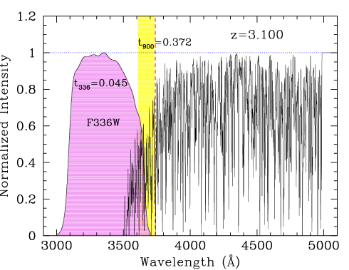
Figure 12.— An example of a single IGM sightline, simulated using the Monte Carlo models described in the appendix, for a source at $z=3.10$. The IGM transmission vs. observed wavelength is shown, with the position of the rest-frame Lyman limit indicated with the vertical dashed red line. The light yellow shaded region illustrates the range of observed wavelength used to calculate $t_{900}$, which in this realization has $t_{900}=0.372$ – close to the mean value expected for $z\sim 3.1$ (see Table 12). The violet shaded region is the filter response function for the HST WFC3/UVIS F336W filter, used for many studies of LyC leakage at $z\lower 2.15277pt\hbox{$\;\buildrel>\over{\sim}\;$}3$. The mean transmitted flux integrated over the F336W bandpass has $t_{F336W}=0.045$, i.e., a factor of $\lower 2.15277pt\hbox{$\;\buildrel>\over{\sim}\;$}8$ lower than the spectroscopic measure of $t_{900}$.

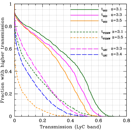
Figure 13.— Comparison of the cumulative distribution of IGM+CGM transmission evaluated for $z_{\rm s}=3.1$ (orange), $z_{\rm s}=3.3$ (magenta), and $z_{\rm s}=3.5$ (green) using the $t_{900}$ bandpass (solid curves) vs. $t_{\rm F336W}$ or $t_{\rm LBC-U}$ (short-dashed curves), where F336W is the WFC3-UVIS filter and LBC-U is the U filter described by Grazian et al. (2016). Note that the largest differences appear at relatively high values of transmission.

There are distinct practical advantages in using a measurement band that samples a fixed bandwidth in the rest frame of each source, 880-910 Å, placed just shortward of the intrinsic Lyman limit. It is possible to use images taken through a comparably-narrow bandpass (i.e., $\simeq 100-200\AA$ in the observed frame; e.g., Inoue & Iwata 2008; Nestor et al. 2011; Mostardi et al. 2013), but a narrow-band filter will be optimally-placed only for sources at a fixed redshift, which as discussed above can also be problematic in terms of sample variance due to gas-phase overdensities and/or correlated sightlines arising in the intra-protocluster medium.

Similar issues affect observations where a broad-band filter is used for the LyC detection band, such as surveys conducted using the F336W filter in the WFC3-UVIS camera on board HST (e.g., Mostardi et al. 2015; Siana et al. 2015; Vasei et al. 2016). In this case, since the broad bandpass must lie entirely shortward of the rest-frame Lyman limit of sources to provide unambiguous detections of ionizing photons, it is confined to source redshifts $z_{\rm s}>3.07$; however, even for $z_{\rm s}\simeq 3.1$, the photon-number-weighted mean flux density measured in the filter bandpass is considerably reduced relative to the rest-frame [880,910] wavelength interval. An example assuming $z_{\rm s}=3.10$ is shown in Figure 12, where $t_{900}=0.372$ (i.e., close to the mean value for random IGM+CGM sightlines to sources with $z_{\rm s}=3.10$; Table 12), but the F336W band-averaged transmission $t_{336}=0.045$, $\sim 8.3$ times smaller (2.3 mag).

Figure 13 shows cumulative distribution functions of $t_{900}$, $t_{336}$, and $t_{\rm LBC}$ (the broadband $U$ filter used by Grazian et al. 2016) for a large ensemble of sightlines to $z_{\rm s}=3.1$ and $z_{\rm s}=3.5$. At $z=3.1$, the median transmission in the relevant LyC detection band is 5.2 times higher using the [880,910] interval than that evaluated through the F336W filter bandpass; the ratio between median transmission values reaches $\sim 200$ by $z=3.5$. The 90th percentile transmission $t_{900}=0.59$ (0.49) for $z_{\rm s}=3.1$ ($z_{\rm s}=3.5$); $t_{336W}=0.38$ (0.14) for $z_{\rm s}=3.1$ ($z_{\rm s}=3.5$). Similarly, compared to the ground-based $U_{\rm LBC}$ used to measure LyC emission from spectroscopically identified galaxies at $z\sim 3.3$ by Grazian et al. (2016, 2017), the spectroscopic [880,910] Å bandpass is $\lower 2.15277pt\hbox{$\;\buildrel>\over{\sim}\;$}2$ times more likely to include sightlines with $t_{\rm LyC}>0.2$, and $\simeq 9$ times more likely to have sightlines with $t_{\rm LyC}>0.4$. These differences could be quite large if there is limited dynamic range for LyC detection from individual sources – as has been the case for all surveys to date – potentially producing large differences in the fraction of sources with significant LyC detections even for surveys that nominally reach the same flux density limit in the LyC band.

Table 5Transmission Statistics vs. LyC Detection Band

LyC Band	$z_{\rm s}$	$\langle t_{LyC}\rangle$	Median	90th Percentile
[880,910]	3.10	0.352	0.393	0.589
HST-F336W	3.10	0.139	0.078	0.377
[880,910]	3.30	0.321	0.359	0.543
LBC-U	3.30	0.149	0.118	0.356
HST-F336W	3.30	0.070	0.017	0.226
[880,910]	3.40	0.291	0.119	0.516
LBC-U	3.40	0.099	0.047	0.282
HST-F336W	3.40	0.050	0.005	0.171
[880,910]	3.50	0.264	0.302	0.492
HST-F336W	3.50	0.039	0.002	0.137

Care must also be exercised when comparing the results of surveys that use different LyC detection bands and/or IGM opacity models: Table 5 compares our determination of the mean IGM+CGM transmission evaluated for 3 different LyC detection passbands. The ensemble of sightlines used at each $z_{\rm s}$ was identical. Note that we find that the mean IGM+CGM transmission evaluated using the $U_{\rm LBC}$ filter for $z_{\rm s}=3.30$ ($z_{\rm s}=3.40$) is $\langle t_{\rm LBC}\rangle\simeq 0.149$ ($0.099$), to be compared with the value assumed by Grazian et al. (2016, 2017), $\langle t_{\rm LBC}\rangle=0.28$. The latter value was based on the IGM opacity models of Inoue et al. (2014). Additional ambiguities relevant to the quantitative comparison of LyC results arise due to differences in the definition of “escape fraction”, discussed in more detail in §9.1.

The main point here is that the probability of detecting LyC emission– or of setting interesting limits on $f_{900}/f_{1500}$– depends very sensitively the source redshift $z_{\rm s}$, the bandwidth and relative wavelength/redshift sensitivity of the LyC detection band, and the fidelity of the correction for the IGM+CGM opacity.

8. Inferences from Composite Spectra of KLCS Galaxies

As discussed in §7, it is potentially misleading to interpret individual measurements of the quantity $(f_{900}/f_{1500})_{\rm obs}$ because of the large expected variation in $t_{900}$ from sightline to sightline. There are significant advantages associated with considering only ensembles of galaxies (sharing particular properties) that are large enough that the uncertainty in the ensemble average IGM correction is reduced. Since we have relatively high quality spectra of 124 objects remaining after cleaning the sample of potential contamination or obvious systematic issues, in this section we combine various subsets of the KLCS spectra to form high S/N spectroscopic composites. The resulting spectra are then used to obtain sensitive measurements of $\langle f_{900}/f_{1500}\rangle_{\rm obs}$ for which $\langle t_{900}\rangle$ is well-determined.

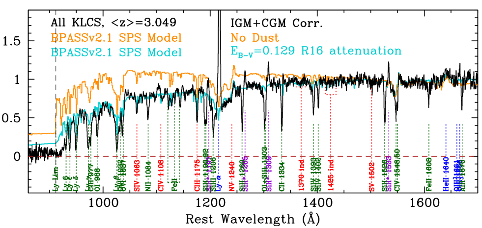
Figure 14.— The composite spectrum of all 124 galaxies included in the KLCS statistical sample (black). The stacked spectrum has been corrected for the mean IGM+CGM opacity appropriate for an ensemble with $\langle z_{\rm s}\rangle=3.05$ as shown in Figure 11. Some of the easily-identified spectral features are indicated, where the labels have been color-coded according to whether they are primarily interstellar (dark green), nebular (blue), stellar (red), or excited fine structure emission (purple). The orange (turquoise) spectrum is the best-fitting stellar population synthesis model (see §9.2) before (after) applying reddening according to Reddy et al. (2016a) (R16).

Figure 15.— Zoomed-in version of Figure 14, showing the composite spectrum formed from all 124 galaxies in the KLCS sample. (Top:) The composite spectrum prior to correction for IGM+CGM opacity, where the measured value of $\langle f_{900}/f_{1500}\rangle_{\rm obs}$ is indicated. (Bottom:) Identical to the top panel, except that here the observed spectrum (black histogram) has been corrected using the model for the average IGM+CGM transmission spectrum (see Fig. 11) appropriate for the KLCS sample distribution of source redshifts. The value of $\langle f_{900}/f_{1500}\rangle_{\rm out}$ given in the bottom panel was calculated using equation 11 (see Table 6.) The values of each, and the wavelength interval over which they have been evaluated, are indicated by magenta bars in both panels. The model spectrum (cyan histogram) is identical in both panels, and also the same as that shown in Figure 14 using the same color coding.

The individual KLCS spectra have a range of S/N owing to differences in apparent magnitude, redshift, and observing conditions. One might be tempted to combine them so as to maximize the S/N of the resulting composite, but the necessary weighting involved would invalidate the approach we adopt to correct for intergalactic opacity, which assumes that every sightline through the IGM is contributing equally to the net suppression of the intrinsic spectrum. Thus, we used the following approach to forming composites.

All extracted one-dimensional spectra (and their associated error spectra) of KLCS galaxies were shifted to the rest frame using the values of $z_{\rm sys}$ (Table 2), where each was resampled to a common wavelength grid using spline interpolation and scaled according to its observed continuum flux density $f_{1500}$. In forming a composite spectrum, the mean value at each rest-wavelength dispersion point was calculated after outliers with values differing by more than $3\sigma$ from the median were rejected. This algorithm is very effective in removing residuals from imperfectly subtracted night sky lines and other defects present in individual spectra. Figure 14 shows the spectroscopic stack of all 124 galaxies in the KLCS analysis sample.

Fig. 14 also addresses the extent to which the IGM opacity models described in §7 are consistent with the attenuation actually observed in the composite galaxy spectrum. The observed spectrum (black) has been corrected using the calculated mean IGM+CGM transmission spectrum appropriate for a sample having $\langle z_{\rm s}\rangle\simeq 3.05$ (Figure 11), normalized so that $\langle f_{1500}\rangle=1$. The orange spectrum is the similarly-normalized intrinsic spectrum of the stellar$+$nebular continuum for the stellar population synthesis (SPS) model found to be most successful in reproducing the observed composite spectrum (see §9.2). The cyan spectrum in Figure 14 is the model SPS spectrum after reddening using the best-fitting attenuation relation and color excess E(B-V) (discussed in §9.2 below) normalized so that $\langle f_{1500}\rangle=1$. Note that the continua of the model spectrum (cyan) and the IGM+CGM-corrected observed spectrum (black) are in excellent agreement over the rest wavelength range 950-1210 Å– the range sensitive to the accuracy of the IGM $\rm Ly\alpha$ forest Monte Carlo modeling vs. redshift (§7 and Appendix B.)

Figure 15 shows a zoomed-in version of Figure 14, illustrating the full KLCS sample before (top panel) and after (bottom panel) applying the IGM+CGM correction to the observed spectrum. The model spectrum shown in each panel is identical, and all spectra have been normalized to unity at rest-frame 1500 Å.

Table 6Statistics Measured from KLCS Composite Spectra

Sample	$N$	$\langle z_{\rm s}\rangle$	$\langle W_{\lambda}(\rm Ly\alpha)\rangle$	$\langle L_{\rm uv}/L_{\rm uv}^{\ast}\rangle$	$(G-{\cal R})_{0}$	$\langle f_{900}/f_{1500}\rangle_{\rm obs}$	${\rm\langle t_{900}\rangle}$	$\langle f_{900}/f_{1500}\rangle_{\rm out}$	${\rm\langle t_{900}\rangle}$	$\langle f_{900}/f_{1500}\rangle_{\rm out}$
			[Å]				[IGM only]	[IGM only]	[IGM+CGM]	[IGM+CGM]
All	124	3.049	$~{}+13.1$	1.04	0.49	$~{}0.021\pm 0.002$	$0.443\pm 0.017$	$0.047\pm 0.005$	$0.368\pm 0.020$	$0.057\pm 0.006$
All, detected	15	3.093	$~{}+29.2$	0.86	0.45	$~{}0.134\pm 0.007$	$\cdots$	$\cdots$	$\cdots$	$\cdots$
All, not detected	106	3.044	$~{}+10.6$	1.07	0.50	$~{}0.010\pm 0.003$	$\cdots$	$\cdots$	$\cdots$	$\cdots$
$z$ (Q1)	31	2.843	$~{}~{}+10.6$	0.91	0.50	$~{}0.022\pm 0.007$	$0.487\pm 0.038$	$~{}0.045\pm 0.015$	$0.412\pm 0.045$	$~{}0.053\pm 0.018$
$z$ (Q4)	31	3.284	$~{}+16.7$	1.18	0.46	$~{}0.019\pm 0.003$	$0.387\pm 0.033$	$~{}0.047\pm 0.009$	$0.321\pm 0.037$	$~{}0.056\pm 0.011$
$L_{\rm uv}>L_{\rm uv}^{\ast}$	60	3.079	$~{}~{}+6.6$	1.44	0.55	$~{}0.002\pm 0.003$	$0.435\pm 0.024$	$~{}0.005\pm 0.007$	$0.363\pm 0.028$	$~{}0.006\pm 0.008$
$L_{\rm uv}<L_{\rm uv}^{\ast}$	64	3.021	$~{}+18.5$	0.67	0.43	$~{}0.042\pm 0.004$	$0.449\pm 0.024$	$~{}0.094\pm 0.010$	$0.372\pm 0.028$	$~{}0.113\pm 0.014$
$L_{\rm uv}$ (Q1)	31	3.064	$~{}~{}+7.4$	1.73	0.53	$~{}0.002\pm 0.003$	$0.438\pm 0.035$	$0.005\pm 0.007$	$0.364\pm 0.040$	$~{}0.005\pm 0.008$
$L_{\rm uv}$ (Q2)	31	3.086	$~{}~{}+5.7$	1.12	0.57	$~{}0.000\pm 0.004$	$0.432\pm 0.035$	$~{}0.000\pm 0.007$	$0.360\pm 0.040$	$~{}0.000\pm 0.011$
$L_{\rm uv}$ (Q3)	31	3.045	$~{}+20.0$	0.81	0.44	$~{}0.042\pm 0.005$	$0.442\pm 0.035$	$~{}0.095\pm 0.014$	$0.367\pm 0.040$	$~{}0.114\pm 0.018$
$L_{\rm uv}$ (Q4)	31	3.001	$~{}+18.1$	0.51	0.42	$~{}0.052\pm 0.007$	$0.453\pm 0.056$	$~{}0.115\pm 0.020$	$0.377\pm 0.042$	$~{}0.138\pm 0.024$
$W_{\lambda}(\rm Ly\alpha)$ (Q1)	31	3.005	$~{}-5.6$	1.13	0.54	$~{}0.005\pm 0.004$	$0.452\pm 0.035$	$~{}0.011\pm 0.009$	$0.378\pm 0.040$	$~{}0.013\pm 0.011$
$W_{\lambda}(\rm Ly\alpha)$ (Q2)	31	3.036	$~{}~{}+2.3$	1.17	0.57	$~{}0.012\pm 0.004$	$0.441\pm 0.035$	$~{}0.027\pm 0.009$	$0.368\pm 0.040$	$~{}0.033\pm 0.011$
$W_{\lambda}(\rm Ly\alpha)$ (Q3)	31	3.055	$~{}~{}+9.3$	0.96	0.47	$~{}0.017\pm 0.005$	$0.440\pm 0.034$	$~{}0.039\pm 0.012$	$0.364\pm 0.040$	$~{}0.047\pm 0.015$
$W_{\lambda}(\rm Ly\alpha)$ (Q4)	31	3.088	$~{}+43.2$	0.92	0.38	$~{}0.058\pm 0.006$	$0.429\pm 0.034$	$~{}0.138\pm 0.018$	$0.355\pm 0.040$	$~{}0.166\pm 0.025$
LAEs	28	3.091	$~{}+44.1$	0.87	0.41	$~{}0.063\pm 0.006$	$0.433\pm 0.036$	$~{}0.145\pm 0.018$	$0.359\pm 0.042$	$~{}0.175\pm 0.026$
non-LAEs	96	3.037	$~{}~{}+3.6$	1.09	0.51	$~{}0.012\pm 0.003$	$0.445\pm 0.020$	$~{}0.027\pm 0.007$	$0.370\pm 0.023$	$~{}0.032\pm 0.008$
$W_{\lambda}(\rm Ly\alpha)>0$	74	3.073	$~{}+22.4$	0.99	0.45	$~{}0.031\pm 0.003$	$0.437\pm 0.022$	$~{}0.071\pm 0.008$	$0.362\pm 0.025$	$~{}0.086\pm 0.010$
$W_{\lambda}(\rm Ly\alpha)<0$	50	3.013	$~{}-3.8$	1.19	0.55	$~{}0.007\pm 0.003$	$0.450\pm 0.027$	$~{}0.016\pm 0.007$	$0.376\pm 0.031$	$~{}0.019\pm 0.008$
$(G-{\cal R})_{0}$ (Q1)	31	3.095	$~{}+19.4$	0.94	0.20	$0.023\pm 0.004$	$0.430\pm 0.034$	$0.053\pm 0.010$	$0.355\pm 0.040$	$0.055\pm 0.013$
$(G-{\cal R})_{0}$ (Q2)	31	3.021	$~{}+15.2$	1.02	0.41	$0.022\pm 0.006$	$0.447\pm 0.035$	$0.049\pm 0.014$	$0.372\pm 0.041$	$0.059\pm 0.017$
$(G-{\cal R})_{0}$ (Q3)	31	3.059	$~{}+12.7$	1.07	0.57	$0.030\pm 0.005$	$0.439\pm 0.035$	$0.068\pm 0.013$	$0.373\pm 0.040$	$0.080\pm 0.016$
$(G-{\cal R})_{0}$ (Q4)	31	3.023	$~{}~{}+4.4$	1.15	0.78	$0.011\pm 0.005$	$0.447\pm 0.035$	$0.025\pm 0.011$	$0.373\pm 0.040$	$0.029\pm 0.016$

8.1. KLCS Subsamples

We formed a number of subsets of the final KLCS statistical sample based on empirical criteria that could be measured easily from photometry or spectroscopy of individual objects; these include $L_{\rm uv}$, $W_{\lambda}(\rm Ly\alpha)$, and rest-UV continuum color $(G-{\cal R})_{0}$ (§6.4). In view of the results of §7.1, a minimum subsample size $N\lower 2.15277pt\hbox{$\;\buildrel>\over{\sim}\;$}30$ was maintained so that the uncertainty in the IGM+CGM correction is $\lower 2.15277pt\hbox{$\;\buildrel<\over{\sim}\;$}10$% (see Table 4). Thus, for each of the aforementioned parameters we split the sample of 124 into 4 independent quartiles consisting of 31 galaxies each.

Additional subsets were formed according to the following criteria: objects with $L_{\rm uv}\geq L_{\rm uv}^{\ast}$ (48% of the sample, very similar to a combination of the $L_{\rm uv}$ (Q1) and $L_{\rm uv}$ (Q2) subsamples) and those with $L_{\rm uv}<L_{\rm uv}^{\ast}$ (52% of the sample); according to whether $\rm Ly\alpha$ appears in net emission ($W_{\lambda}(\rm Ly\alpha)>0$; 60% of the sample) or net absorption ($W_{\lambda}(\rm Ly\alpha)\leq 0$; 40% of the sample); and, finally, grouping together the galaxies exceeding the often-used threshold $W_{\lambda}(\rm Ly\alpha)>20$ Å for “Lyman Alpha Emitters” (LAEs). The KLCS LAE sub-sample (28 galaxies, or $\simeq 22.6$% of the total) is based upon the spectroscopically-measured $W_{\lambda}(\rm Ly\alpha)$, and happens to be nearly identical to the $W_{\lambda}(\rm Ly\alpha)$ (Q4) sub-sample of 31 galaxies.

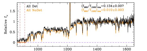
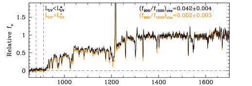
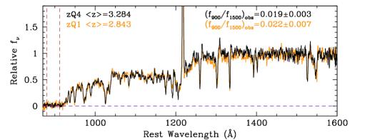
Figure 16.— Composite rest-frame spectra of selected KLCS sub-samples, normalized so that $f_{1500}=1.0$. No IGM correction has been applied, i.e., they are the observed flux density as a function of rest wavelength. The subsample names are indicated (color-coded) in the top left corner of each panel, with the corresponding measurements of $\langle f_{900}/f_{1500}\rangle_{\rm obs}$ in the upper right of each panel. The vertical dashed lines mark the [880,910] rest wavelength interval used for measuring $f_{900}$.

Table 6 includes values of parameters measured directly from the composite spectra or the mean value among the objects comprising the subsample: the number of galaxies in the subsample ($N$), the mean redshift of the objects in the subsample ($\langle z_{\rm s}\rangle$), $W_{\lambda}(\rm Ly\alpha)$ (measured directly from the composite spectrum), the mean UV luminosity relative to $L_{\rm uv}^{\ast}$ ($\langle L_{\rm uv}/L_{uv}^{\ast}\rangle$), and the measured flux density ratio $\langle f_{900}/f_{1500}\rangle_{\rm obs}$. Values of $\langle t_{900}\rangle$ for the transmission in the rest wavelength range [880,910] Å are given for both the “IGM only” and “IGM+CGM” Monte Carlo models (§7 and Appendix B), where each value and its uncertainty were calculated by drawing ensembles of sightlines with the same number and $z_{\rm s}$ distribution as the subsample, averaging the values of $t_{900}$, and repeating 1000 times. The tabulated uncertainties reflect the 68% confidence interval for the mean transmission of the 1000 ensembles for each subsample. The composite spectra of several of the sub-samples listed in Table 6 are shown in Figure 16.

The corrected (emergent) flux density ratio $\langle f_{900}/f_{1500}\rangle_{\rm out}$ (equation 11) is also listed in Table 6, where the quoted errors include uncertainties in both the measurement and in $\langle t_{900}\rangle$. Table 6 also includes entries for the full KLCS sample (“All”), and “All” divided into subsets according to whether or not the individual LyC measurement had $|f_{900}/\sigma_{900}|>3$.

Finally, Table 6 includes entries for subsamples of KLCS formed according to $z_{\rm s}$, where $z_{\rm s}$ (Q1) is the lowest-redshift quartile, and $z_{\rm s}$ (Q4) the highest-redshift quartile. These are intended to show that there is no strong dependence of the results on source redshift once the redshift-dependent IGM (or IGM+CGM) corrections have been applied; the composite spectra of these two redshift subsamples are among those shown in Figure 16.

8.2. Assessment of LyC Results

Figure 17.— (Top:) Inferred values of $\langle f_{900}/f_{1500}\rangle_{\rm out}$ versus UV luminosity relative to $L_{\rm uv}^{\ast}$ at $z\sim 3$. The four independent quartiles in luminosity are indicated turquoise points surrounded by black circles; other subsamples are plotted for reference. (Bottom:) As for the top panel, but showing $\langle f_{900}/f_{1500}\rangle_{\rm out}$ as a function of the rest equivalent width of the $\rm Ly\alpha$ line in the composite spectrum. The independent quartiles in $W_{\lambda}(\rm Ly\alpha)$ are marked with magenta points surrounded by black circles, with other composite sub-samples included for reference, labeled according to their designation in Table 6. The error bars in both panels include both measurement uncertainties and sample variance in the IGM+CGM correction (the latter depends on the size and redshift distribution of the sub-sample). The error bars on the $\langle f_{900}/f_{1500}\rangle_{\rm out}$ “IGM-only” points (open circles) have been suppressed for clarity in both panels; the values are listed in Table 6. In the bottom panel, the dashed (magenta) line is a linear relation of the form $\langle f_{900}/f_{1500}\rangle_{\rm out}$$=0.36(W_{\lambda}/110~{}\textrm{\AA})+0.02$.

On the basis of the results summarized in Table 6, there are two easily-measured empirical characteristics that correlate most strongly with a propensity to “leak” measurable LyC radiation: $L_{\rm uv}$ and $W_{\lambda}(\rm Ly\alpha)$. Figure 17 illustrates, for selected sub-samples indicated on the figure, the dependence on $L_{\rm uv}$ and $W_{\lambda}(\rm Ly\alpha)$ of the measured $\langle f_{900}/f_{1500}\rangle_{\rm obs}$ and inferred $\langle f_{900}/f_{1500}\rangle_{\rm out}$ for both IGM transmission models.

The top panel of Figure 17 suggests an almost bimodal dependence of $\langle f_{900}/f_{1500}\rangle_{\rm out}$ on $L_{\rm uv}$, where the 2 lowest-luminosity quartiles (i.e., the lower luminosity half) of the KLCS sample have $\langle f_{900}/f_{1500}\rangle_{\rm out}$$\simeq 0.13$, whereas the UV-brighter half of the sample has $\langle f_{900}/f_{1500}\rangle_{\rm out}$ consistent with zero ($3\sigma$ upper limit $\langle f_{900}/f_{1500}\rangle_{\rm out}$$\lower 2.15277pt\hbox{$\;\buildrel<\over{\sim}\;$}0.02$.) The transition luminosity below which $\langle f_{900}/f_{1500}\rangle_{\rm out}$ appears to increase from zero to $\simeq 13$% is very close to $L_{\rm uv}^{\ast}$, which also happens to lie close to the median $L_{\rm uv}$ of the KLCS sample.

The trend of $\langle f_{900}/f_{1500}\rangle_{\rm obs}$ and $\langle f_{900}/f_{1500}\rangle_{\rm out}$ with $W_{\lambda}(\rm Ly\alpha)$ – illustrated in the bottom panel of Figure 17 – is similar, albeit perhaps exhibiting a more gradual dependence of $\langle f_{900}/f_{1500}\rangle_{\rm out}$ on $W_{\lambda}(\rm Ly\alpha)$ compared to the relatively abrupt luminosity dependence of the subsamples grouped according to $L_{\rm uv}$.

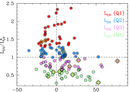
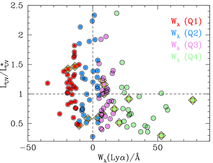
Figure 18.— (Top:) $L_{\rm uv}/L_{\rm uv}^{\ast}$ versus the rest-frame $\rm Ly\alpha$ ($W_{\lambda}(\rm Ly\alpha)$) for the KLCS sample. The points have been color-coded by quartiles in $L_{\rm uv}$: from lower to higher luminosity, pale green (Q4), violet (Q3), blue (Q2), and red (Q1). (Bottom:) Same as the top panel, except with points color-coded by quartiles in $W_{\lambda}(\rm Ly\alpha)$. In both panels, the galaxies with $3\sigma$ LyC detections are also indicated with diamonds.

Figure 18 shows the KLCS sample color-coded according to quartiles in $L_{\rm uv}$ (top) and $W_{\lambda}(\rm Ly\alpha)$ (bottom). There is clearly an inverse correlation between $W_{\lambda}(\rm Ly\alpha)$ and $L_{\rm uv}$ in the sense that there is a dearth of galaxies with bright $L_{\rm uv}$ and large $W_{\lambda}(\rm Ly\alpha)$ – e.g., the brighter two quartiles in $L_{\rm uv}$ (Q1 and Q2) are dominated by galaxies with $W_{\lambda}(\rm Ly\alpha)$$\lower 2.15277pt\hbox{$\;\buildrel<\over{\sim}\;$}10$ Å (median$\simeq 0$ Å), and most of the galaxies in the two largest-$W_{\lambda}(\rm Ly\alpha)$ quartiles (Q3 and Q4) have $L_{\rm uv}<L_{\rm uv}^{\ast}$. Because of the well-established correlation between $L_{\rm uv}$ and $W_{\lambda}(\rm Ly\alpha)$ within all LBG samples (including KLCS; see ,e.g., Shapley et al. 2003; Gronwall et al. 2007; Kornei et al. 2010; Stark et al. 2010), it is difficult to say with certainty which is the more reliable indicator of high $\langle f_{900}/f_{1500}\rangle_{\rm out}$; however, for reasons discussed in detail in §9.3 and §11.1 below, we believe that $W_{\lambda}(\rm Ly\alpha)$ is more directly linked to whether or not a galaxy has significant LyC leakage, and that the $L_{\rm uv}$ dependence of $\langle f_{900}/f_{1500}\rangle_{\rm out}$ results from the UV luminosity dependence of the gas-phase covering fraction/column density along the line of sight.

9. Galaxy Properties and LyC Escape

While a determination of the total ionizing emissivity contributed by an ensemble of galaxies can be calculated directly from $\langle f_{900}/f_{1500}\rangle_{\rm out}$, without knowing anything about the galaxies except for their FUV luminosity function, one would like to understand the physical causes of the large differences inferred among the sample. More generally, one would like to place LyC escape in the context of other galaxy properties, including the massive star populations and the ISM conditions that modulate LyC “leakage”. Understanding which galaxies contribute – and why – to the metagalactic ionizing radiation field at $z\sim 3$ will certainly improve our ability to make quantitative sense of the reionization era, where direct measurements of $\langle f_{900}/f_{1500}\rangle_{\rm out}$ will not be possible. These questions also bear considerably on our understanding of galaxies, the CGM, and the IGM at $z\sim 3$ where the impact of LyC leakage is direct and highly relevant. In this section, we extend our analysis of the KLCS results to include properties of the galaxies, their stellar populations, and the radiative transfer of ionizing and non-ionizing FUV light through the ISM.

We begin by briefly reviewing the commonly-used forms of the LyC “escape fraction” ($f_{\rm esc}$) in the context of the KLCS dataset.

9.1. Escape Fraction: Definitions

The most common definition of escape fraction, often used in theoretical studies of re-ionization, is the fraction of ionizing photons produced by stars in a galaxy that escape into the IGM without being absorbed by H I within the galaxy (e.g., Wyithe & Cen 2007; Wise & Cen 2009). This quantity has also been called the “absolute escape fraction” ($f_{\rm esc,abs}$) to convey the fact that the ionizing photon budget against which the leaking LyC is compared includes all of the ionizing UV photons whether or not they are evident in observations. Thus, in order to determine $f_{\rm esc,abs}$, a measure of the intrinsic production rate of ionizing photons is necessary; unfortunately, direct empirical estimates of the production rate of ionizing photons ($N_{\rm ion}$) are relatively impractical for high redshift galaxies. Instead, one typically uses SED modeling of young stellar populations (including dust extinction, population age, IMF, etc.) to estimate the intrinsic ionizing photon production. Doing this accurately requires knowledge of the intrinsic SED of the massive stellar populations in the extreme UV (EUV), especially for photon energies in the range 1-4 Ryd, as well as a detailed understanding of the distribution and composition of dust grains that attenuate and redden the intrinsic spectrum of the stars in the galaxy.

An alternative definition intended to be closer to the most readily-available measurements of high redshift galaxy populations is the “relative escape fraction” ($f_{\rm esc,rel}$; Steidel et al. 2001),

$$f_{\rm esc,rel}=\frac{\langle f_{900}/f_{1500}\rangle_{\rm out}}{(L_{900}/L_{1500})_{\rm int}}\times 10^{\left[A_{\lambda}(900)-A_{\lambda}(1500)\right]/2.5}$$ (12)

where

$$A_{\lambda}=k_{\lambda}E(B-V)\quad.$$ (13)

is the attenuation in magnitudes as a function of rest wavelength and $k_{\lambda}$ parametrizes the attenuation relation. The term $(L_{900}/L_{1500})_{\rm int}$ is the intrinsic ratio of the unattenuated stellar population of the galaxy, prior to transfer through the ISM, the CGM, and the IGM. Note that there are inconsistencies in the definition of $f_{\rm esc,rel}$ in the literature having to do with whether or not dust attenuation is included; some authors have implicitly assumed that $A_{\lambda}(900)-A_{\lambda}(1500)=0$, i.e. that the attenuation by dust affects ionizing and non-ionizing UV equally, or that dust affects only the non-ionizing UV [i.e., $A_{\lambda}(900~{}\textrm{\AA})=0$]. The definition of $f_{\rm esc,rel}$ used by Grazian et al. (2017), expressed using the notation we have adopted here, is $f_{\rm esc,rel}=(f_{900}/f_{1500})_{\rm out}/(L_{900}/L_{1500})_{\rm int}$. In order to avoid ambiguity, in what follows below we have attempted to be clear about any assumptions made in mapping $\langle f_{900}/f_{1500}\rangle_{\rm out}$ to more model-dependent quantities whenever relevant; §9.4.1 and 9.4.2 consider ISM models both with and without dust attenuation of emergent LyC flux.

9.2. Stellar Population Synthesis Models

The intrinsic energy distribution of the stellar sources, parametrized by $(L_{900}/L_{1500})_{\rm int}$, is a crucial ingredient to understanding the relationship between ionizing photon production and escape into the IGM. The intrinsic break at the Lyman limit in the integrated spectrum of stars depends on the age, metallicity, initial mass function (both slope and upper mass limit), and the effects of binary evolution of massive stars. Depending on the assumptions, SPS models predict spectra falling in the range $0.15\lower 2.15277pt\hbox{$\;\buildrel<\over{\sim}\;$}(L_{900}/L_{1500})_{\rm int}\lower 2.15277pt\hbox{$\;\buildrel<\over{\sim}\;$}0.75$ (see, e.g., Leitherer et al. 1999; Eldridge et al. 2017). In the absence of external constraints, the factor of $\sim 5$ uncertainty on $(L_{900}/L_{1500})_{\rm int}$ translates directly into uncertainties on estimates of escape fraction.

Fortunately, high quality far-UV composite spectra such as those of the KLCS sub-samples significantly constrain the likely range of stellar population parameters consistent with the observations. Using similar far-UV composites constructed from the spectra of $\langle z\rangle\simeq 2.4$ galaxies that were also observed in the near-IR as part of KBSS-MOSFIRE, Steidel et al. (2016) (S16) showed that, among the SPS models considered, the only set which could simultaneously match the details of the far-UV stellar spectrum – and correctly match the observed ratios of strong nebular emission lines in the spectra of the same galaxies – were those with low stellar metallicity, ${\rm(Fe/H)\simeq 0.1~{}(Fe/H)_{\odot}}$, and which include the evolution of massive stars in binary systems (BPASSv2.1; Eldridge et al. 2017).

Prior to fitting models to the observed spectra, the mean IGM transmission spectrum for the CGM+IGM Monte Carlo models described in §7 and Appendix B (similar to that shown in Figure 11) were calculated separately for each subsample by drawing 1000 sightline ensembles with the same number and $z_{\rm s}$ distribution. We divided the observed subsample spectrum by the mean transmission spectrum and propagated the 68% confidence interval around the mean at each rest-wavelength point as the contribution of the IGM correction to the error vector for $\lambda_{0}<1216$ Å.

Following the procedure detailed in S16, we fit each of the composite KLCS spectra in Table 6 with a range of SPS models similar to that described by S16, with the following additions: we tested 3 different attenuation relations for reddening the SPS model spectra, in addition to varying the metallicity of the stars and the upper mass limit and slope of the IMF. We found that the newest publicly released BPASSv2.1 (Eldridge et al. 2017) models with stellar metallicity $Z_{\ast}=0.001$ ($\simeq 0.07~{}Z_{\odot}$, assuming the solar abundance scale of Asplund et al. 2009), IMF slope $\alpha=-2.35$, and upper stellar mass limit of 300 M_⊙ (hereafter referred to as BPASSv2.1-300bin-z001), provided the lowest $\chi^{2}$ (i.e., the best fit) for every KLCS composite listed in Table 6. For all of the fits, we assumed a continuous star formation history, constant star formation rate, and an age of $t=10^{8}$ years, close to the median age inferred from SED fits to photometry from the UV to mid-IR (e.g., Reddy et al. 2012; Du et al. 2018.) The effects of the star-forming age on the EUV-FUV spectra in the context of the BPASS-v2.1-300bin-z001 models are discussed in §10. The continuum reddening was allowed to vary over the range $0\leq E(B-V)<1.0$ for each subsample; however, the attenuation relation accompanying the best-fitting model varied among the sub-samples; Table 7 summarizes the parameters of the best fit for each sub-sample listed in Table 6.

Table 7Statistics Derived from SPS Model Fits to Spectra

Sample	Att.	E(B-V)	$(L_{900}/L_{1500})_{\rm mod}$	C1500	$\langle L_{\rm bol}\rangle$	$\langle f_{\rm esc,rel}\rangle$	$\langle f_{\rm esc,abs}\rangle$	$\langle f_{\rm esc,rel}\rangle$	$\langle f_{\rm esc,abs}\rangle$
					($10^{11}L_{\rm\odot}$)	[IGM only]		[IGM+CGM]
All	R16	0.129	0.167	2.88	2.98	$0.29\pm 0.03$	$0.09\pm 0.01$	$~{}0.36\pm 0.04$	$~{}0.12\pm 0.01$
All, detected	SMC	0.045	0.183	1.76	1.50	$1.04\pm 0.10$	$0.60\pm 0.06$	$~{}1.21\pm 0.11$	$~{}0.70\pm 0.07$
All, not detected	R16	0.135	0.163	3.03	3.17	$0.13\pm 0.04$	$0.04\pm 0.01$	$~{}0.17\pm 0.05$	$0.06\pm 0.02$
z(Q1)	SMC	0.060	0.160	2.12	1.92	$0.27\pm 0.08$	$0.12\pm 0.04$	$~{}0.34\pm 0.11$	$~{}0.16\pm 0.03$
z(Q4)	R16	0.080	0.202	1.93	2.26	$0.25\pm 0.04$	$0.12\pm 0.02$	$~{}0.31\pm 0.05$	$~{}0.16\pm 0.03$
$L_{\rm uv}>L_{\rm uv}^{\ast}$	R16	0.141	0.160	3.18	4.55	$0.03\pm 0.04$	$0.01\pm 0.01$	$~{}0.05\pm 0.05$	$~{}0.02\pm 0.02$
$L_{\rm uv}<L_{\rm uv}^{\ast}$	SMC	0.047	0.180	1.80	1.20	$0.52\pm 0.04$	$0.27\pm 0.03$	$~{}0.66\pm 0.09$	$~{}0.36\pm 0.04$
$L_{\rm uv}$ (Q1)	R16	0.133	0.165	2.98	5.11	$0.01\pm 0.04$	$0.02\pm 0.01$	$0.03\pm 0.05$	$~{}0.01\pm 0.02$
$L_{\rm uv}$ (Q2)	R16	0.154	0.152	3.54	3.94	$-0.01\pm 0.06$	$0.00\pm 0.02$	$-0.01\pm 0.07$	$-0.00\pm 0.02$
$L_{\rm uv}$ (Q3)	SMC	0.047	0.180	1.80	1.44	$0.54\pm 0.07$	$0.29\pm 0.04$	$0.67\pm 0.10$	$~{}0.38\pm 0.05$
$L_{\rm uv}$ (Q4)	SMC	0.044	0.185	1.73	0.88	$0.62\pm 0.11$	$0.34\pm 0.07$	$0.79\pm 0.13$	$~{}0.45\pm 0.07$
$W_{\lambda}(\rm Ly\alpha)$ (Q1)	R16	0.158	0.150	3.66	4.10	$0.07\pm 0.06$	$0.02\pm 0.02$	$~{}0.08\pm 0.07$	$~{}0.02\pm 0.02$
$W_{\lambda}(\rm Ly\alpha)$ (Q2)	R16	0.176	0.140	4.24	4.93	$0.21\pm 0.06$	$0.05\pm 0.02$	$~{}0.26\pm 0.08$	$~{}0.06\pm 0.02$
$W_{\lambda}(\rm Ly\alpha)$ (Q3)	SMC	0.049	0.177	1.85	1.76	$0.21\pm 0.07$	$0.11\pm 0.04$	$~{}0.26\pm 0.08$	$~{}0.14\pm 0.05$
$W_{\lambda}(\rm Ly\alpha)$ (Q4)	SMC	0.027	0.215	1.40	1.29	$0.61\pm 0.08$	$0.43\pm 0.06$	$~{}0.76\pm 0.11$	$~{}0.55\pm 0.08$
LAEs	SMC	0.027	0.215	1.40	1.21	$0.66\pm 0.08$	$0.46\pm 0.06$	$~{}0.85\pm 0.12$	$~{}0.62\pm 0.09$
non-LAEs	R16	0.146	0.157	3.31	3.58	$0.19\pm 0.04$	$0.05\pm 0.01$	$~{}0.23\pm 0.05$	$~{}0.07\pm 0.02$
$W_{\lambda}(\rm Ly\alpha)>0$	SMC	0.042	0.188	1.69	1.66	$0.37\pm 0.04$	$0.21\pm 0.03$	$~{}0.48\pm 0.05$	$~{}0.28\pm 0.03$
$W_{\lambda}(\rm Ly\alpha)<0$	R16	0.165	0.146	3.87	4.57	$0.11\pm 0.05$	$0.03\pm 0.01$	$~{}0.13\pm 0.05$	$~{}0.03\pm 0.01$
$(G-{\cal R})_{0}$ (Q1)	SMC	0.015	0.240	1.21	1.12	$0.21\pm 0.04$	$0.17\pm 0.03$	$~{}0.28\pm 0.05$	$~{}0.23\pm 0.04$
$(G-{\cal R})_{0}$ (Q2)	R16	0.113	0.178	2.53	2.56	$0.26\pm 0.08$	$0.10\pm 0.03$	$~{}0.33\pm 0.10$	$~{}0.13\pm 0.04$
$(G-{\cal R})_{0}$ (Q3)	R16	0.159	0.149	3.69	3.91	$0.48\pm 0.09$	$0.12\pm 0.02$	$~{}0.60\pm 0.11$	$~{}0.16\pm 0.03$
$(G-{\cal R})_{0}$ (Q4)	R16	0.221	0.117	6.13	7.00	$0.19\pm 0.12$	$0.03\pm 0.02$	$~{}0.25\pm 0.14$	$~{}0.04\pm 0.02$

Although three different attenuation relations were tested in the fitting, none of the composite spectra was best-fit by the Calzetti et al. (2000) attenuation relation. As indicated in Table 7, 13 of the 23 composite spectra were best fit by the attenuation relation constructed by combining the results of Reddy et al. (2015) with the far-UV extension of Reddy et al. (2016a) (R16), while the remaining 10 spectra favored the steeper, SMC attenuation curve which combines the empirical line-of-sight SMC extinction curve from Gordon et al. (2003) (assuming $R_{\rm V}=2.74$) with an extension to the FUV derived as in Reddy et al. (2016a).

The values of $(L_{900}/L_{1500})_{\rm mod}$ listed in Table 7 assume (for the time being) that the same attenuation curve and $E(B-V)$ value affects both the ionizing and non-ionizing UV light, and that the far-UV attenuation curves can be extrapolated shortward of $\lambda_{0}\leq 950$ Å, the shortest wavelength over which they are empirically constrained (see Reddy et al. 2016a). Here we remind the reader that the values of $\langle f_{\rm esc,rel}\rangle$ listed in Table 7 are as defined in equation 12. Although the fits to the stellar continuum exclude all wavelength pixels shortward of 1070 Å, the fitted spectra appear to be excellent representations of the observed spectra all the way down to $\sim 930$ Å, where the confluence of the stellar and interstellar Lyman series lines in the wavelength interval $910-930$ Å depresses the galaxy spectrum relative to the model; an example is shown in Figures 14 (see also Figure 15.)

The BPASSv2.1-300bin-z001 continuous star formation SPS model, including the contribution of the nebular continuum as described by S16, has $(L_{900}/L_{1500})_{\rm int}\simeq 0.28\pm 0.03$, prior to reddening according to the values in Table 7; our assumption that the entire spectrum is reddened by the same attenuation relation further reduces the intrinsic $L_{900}/L_{1500}$ by an amount that depends on $E(B-V)$ and the attenuation curve. Thus, the values of $(L_{900}/L_{1500})_{\rm mod}$ in Table 7 correspond to the predicted emergent spectrum that would be observed if there were reddening by dust, but no photoelectric absorption by H I in the ISM along the line of sight.

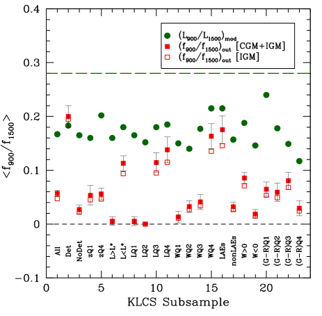
Figure 19.— Comparison of IGM+CGM (filled red squares with error bars) and IGM-only (open red squares) of $\langle f_{900}/f_{1500}\rangle_{\rm out}$ (see Table 6), with the values of $(L_{900}/L_{1500})_{\rm mod}$ based on the best-fit continuum-reddened stellar population synthesis model. The ratio between the values of the red (squares) and filled green dots is defined as $f_{\rm esc,rel}$ (Table 7). The error bars on the IGM-only points (open squares) have been suppressed for clarity (see Table 6 for values). The dashed horizontal line shows the value of $(L_{900}/L_{1500})_{\rm int}$ for the SPS model.

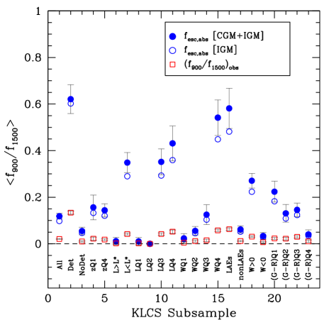
Figure 20.— Comparison of the inferred value of $f_{\rm esc,abs}\equiv f_{\rm esc,rel}/{\rm C}1500$ (solid and open blue circles) with the observed ratio (open red squares) $(f_{900}/f_{1500})_{\rm obs}$ (see Table 6). As for Figure 19, the error bars have been suppressed for $f_{\rm esc,abs}$ values for the “IGM-only” opacity model; the values of the points are collected in Table 7.

Table 7 lists the inferred values of $f_{\rm esc,rel}$, equal to the ratio between $\langle f_{900}/f_{1500}\rangle_{\rm out}$ (Table 6) and $(L_{900}/L_{1500})_{\rm mod}$ (see equation 12), the flux density ratio for the best-fit (reddened) SPS spectrum. Figure 19 illustrates the associated values for each of the subsample composite spectra.

At this point, the value of $f_{\rm esc,rel}$ has accounted for the relative attenuation between $900$ and $1500$ Å, but not for the absolute attenuation affecting $f_{1500}$. In the context of the modeled UV SEDs summarized in Table 7, this factor is simply

$${\rm C1500}\equiv 10^{E(B-V)\times k_{\lambda}(1500)/2.5}$$ (14)

where $k_{\lambda}(1500)=8.91,13.05$ for the R16 and SMC attenuation relations, respectively.

We then define the absolute escape fraction as

$$\langle f_{\rm esc,abs}\rangle=\langle f_{\rm esc,rel}\rangle/{\rm C1500}~{};$$ (15)

both ${\rm C1500}$ and $f_{\rm esc,abs}$ are included in Table 7. Figure 20 compares the values of this inferred quantity with the observed $\langle f_{900}/f_{1500}\rangle_{\rm obs}$ for each KLCS subset composite spectrum. Note that all of the KLCS subsets with $f_{\rm esc,abs}\lower 2.15277pt\hbox{$\;\buildrel>\over{\sim}\;$}0.20$ – whether based on UV color, UV luminosity, or $W_{\lambda}(\rm Ly\alpha)$ – are best-fit using the “line-of-sight” SMC extinction curve. This can probably be attributed to the relatively blue UV color of these composites, as the bluest/youngest star forming galaxies are known to be most consistent with a steep UV attenuation curve (Reddy et al. 2010, 2017), rather than grayer extinction curves such as those of Calzetti et al. (2000) or Reddy et al. (2016a), perhaps due to the prevalence of small dust grains (or the absence of large ones).

We note that fitting reddened SPS models to the observed spectra to estimate $f_{\rm esc,abs}$ (Table 7 and Figure 20) rather than the more empirical $\langle f_{900}/f_{1500}\rangle_{\rm out}$ reveals that, in addition to luminosity and $W_{\lambda}(\rm Ly\alpha)$ dependence noted in §8 for $\langle f_{900}/f_{1500}\rangle_{\rm out}$ (each of which becomes steeper relative to $f_{\rm esc,abs}$), accounting for continuum reddening corrections suggests that $f_{\rm esc,abs}$ also depends strongly on UV color ($(G-{\cal R})_{0}$), in qualitative agreement with the analysis presented by Reddy et al. (2016b).

We return to a discussion of the implications of the various measures of escape fraction in §12.

9.3. Far-UV Spectral Properties and LyC Escape

As described in §9.2 above, the relative escape fraction is $f_{\rm esc,rel}\simeq 0.5$ for the most-leaking KLCS subsets, with corresponding $f_{\rm esc,abs}\simeq 0.3-0.4$; both values are model-dependent in the sense that they are evaluated relative to assumed SPS models (whereas $(f_{900}/f_{1500})_{\rm out}$ is SPS model-independent). We have shown that there is a strong correlation between $W_{\lambda}(\rm Ly\alpha)$ and $f_{\rm esc}$, and it has been known for some time (Shapley et al. 2003) that $W_{\lambda}(\rm Ly\alpha)$ is anti-correlated with the strength of low-ionization (e.g., C II, Si II, O I) interstellar absorption features observed in the same spectra. The presence of strong lines of neutral and singly-ionized species in gas seen in absorption against the UV continuum from massive stars suggests significant neutral H column densities, $N_{\rm HI}>10^{17}$ cm^-2, and the relatively constant $W_{\lambda}/\lambda$ for lines of the same species but varying $\lambda f$, where $\lambda$ is the rest wavelength of the transition and $f$ is the oscillator strength (e.g., Si II $\lambda 1190$, 1193, 1260, 1304, 1526) indicates the presence of saturation.

The observation that strong IS lines often do not become black at maximum optical depth then suggests partial covering of the continuum source (hereinafter, $f_{\rm c}<1$) by the low-ion-bearing gas. If the same partial covering were to apply to the H I, there would follow an obvious relationship between gas covering fraction $f_{\rm c}$ and the probability that significant LyC could “escape” via the uncovered regions. Conversely, if a galaxy spectrum’s low-ionization IS lines are black over a considerable range in velocity, one would expect no significant LyC photon leakage in our direction (e.g., Steidel et al. 2001; Pettini et al. 2002; Shapley et al. 2003, 2006; Quider et al. 2009; Steidel et al. 2010; Heckman et al. 2011; Jones et al. 2012). However, as recently shown (Henry et al. 2015; Vasei et al. 2016; Reddy et al. 2016b), $f_{c}<1$ for low-ionization metal lines is a necessary, but not sufficient, predictor of significant LyC leakage from a galaxy. The metal lines would be relatively insensitive to low-metallicity H I, and possibly also to metal-enriched gas with LyC optical depths $1\lower 2.15277pt\hbox{$\;\buildrel<\over{\sim}\;$}\tau_{\rm LyC}\lower 2.15277pt\hbox{$\;\buildrel<\over{\sim}\;$}10$ where neutral and singly-ionized metallic species might not be the dominant ionization stages in the gas (see also Rivera-Thorsen et al. 2015.)

To examine trends in the residual depth and the velocity extent of interstellar absorption features, we divided each of the KLCS composites by its best-fit SPS model, and formed continuum-normalized spectra with the strongest stellar features removed. Figure 21 shows the line profiles of Si II $\lambda 1260$ and $\lambda 1526$, C II $\lambda 1334$, and the Ly$\beta$ $\lambda 1025.7$ and Ly$\epsilon$ $\lambda 937.8$ for several of the KLCS subsets. Also shown in each panel of Figure 21 is the profile of $\rm Ly\alpha$ emission, after subtracting the stellar continuum, dividing by a factor of 15, and adding 1 (both of the latter for display purposes). The spectral resolution (FWHM) for the metal lines (labeled “LRIS-R”) and for the Lyman lines (labeled “LRIS-B”) are shown in the bottom right of each panel. Figure 21 is arranged according to the measured $f_{\rm esc,abs}$, from largest (top left) to smallest (bottom right).

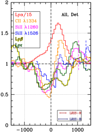
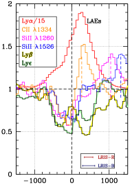
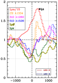
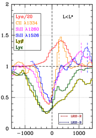
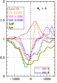
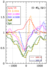
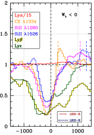
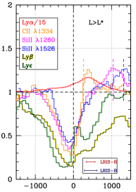
Figure 21.— Profiles of normalized intensity vs. systemic velocity for selected IS absorption lines for selected KLCS sub-samples after normalizing by the best-fit SPS model as described in §9.2: C II $\lambda 1334.5$ (orange), Si II $\lambda 1260.4$ (magenta), Si II $\lambda 1526.7$ (blue), Ly$\beta$$~{}\lambda 1025.7$ (yellow), Ly$\epsilon~{}\lambda 937.8$ (pale green), and $\rm Ly\alpha$ emission (red). The panels are arranged (left to right and top to bottom) in order of decreasing $f_{\rm esc,abs}$ (last column of Table 7.) $\rm Ly\alpha$ emission profiles are based on the SPS continuum-subtracted spectrum; each has been scaled down by a factor of 15 and shifted by +1.0 for display purposes. The three additional emission profiles at velocities $>0$ km s${}^{-1}\,$ are non-resonant emission lines C II${}^{\ast}~{}\lambda 1335.7$ (orange), Si II${}^{\ast}~{}\lambda 1264.8$ (magenta), and Si II${}^{\ast}~{}\lambda 1533.4$ (blue). Short vertical dashed lines, color coded in the same way, mark the position of $v_{\rm sys}=0$. The legend in the lower right of each panel shows the approximate spectral resolution for LRIS-R (relevant for the metal lines) and LRIS-B (relevant for the Lyman series lines).

In addition to the trends already noted between $W_{\lambda}(\rm Ly\alpha)$ and $\langle f_{900}/f_{1500}\rangle_{\rm out}$, there is a similar trend between the apparent depth of the Lyman series and low-ionization metallic absorption lines and $f_{\rm esc}$. In this context, it is noteworthy that the metallic lines shown in Figure 21 were recorded using LRIS-R, which have (as discussed in §3) spectral resolving power $R\sim 1400$ ($\sigma_{\rm inst}\simeq 90$ km s${}^{-1}\,$), whereas the Ly series absorption lines were measured using LRIS-B, with $R\sim 800$ ($\sigma_{\rm inst}\simeq 160$ km s${}^{-1}\,$). In spite of this, the Lyman series absorption lines in all cases have equal or larger apparent optical depth than the metal lines. The similarity of the apparent depth of Lyman lines (at least, for $v_{\rm sys}\lower 2.15277pt\hbox{$\;\buildrel<\over{\sim}\;$}0$) in all of the composites shown suggests ${\rm log(N_{\rm HI}/cm^{2})}\lower 2.15277pt\hbox{$\;\buildrel>\over{\sim}\;$}18$ – in which case all of the observed Ly lines would be strongly saturated – coupled with partial covering of the far-UV continuum. In general, the maximum depths of both H I and metallic absorption lines occur at $-300\lower 2.15277pt\hbox{$\;\buildrel<\over{\sim}\;$}v\lower 2.15277pt\hbox{$\;\buildrel<\over{\sim}\;$}-100$ km s${}^{-1}\,$, consistent with the hypothesis that the bulk of the cool, metal-enriched gas along the sightline “down the barrel” is out-flowing. The Ly line profiles exhibit more varied behavior for velocities $v>0$, where absorption is less-deep overall, and where Ly$\beta$ absorption is significantly stronger than Ly$\epsilon$, suggesting that both $f_{\rm c}$ and ${\rm log(N_{\rm HI})}$ are lower for gas with $v>0$ physically located on the near-side of the stars comprising the UV continuum.

The shapes and depths of the metal lines at $v>0$ are difficult to interpret in the same way, since all of the metallic species shown in Fig. 21 are resonance lines that may manifest “emission filling” from scattered line photons re-emitted in our direction (see, e.g., Prochaska et al. 2011; Erb et al. 2012; Martin et al. 2012; Scarlata & Panagia 2015). However, all 3 of the lines illustrated have nearby non-resonant transitions (i.e., transitions from the same excited state to excited fine structure levels just above the ground state) which can act as “relief valves” for the resonance lines, so that a substantial fraction of absorbed resonance photons may be re-emitted in the non-resonance emission lines – in this case, Si II${}^{\ast}\lambda 1264.9$, C II${}^{\ast}\lambda 1335.7$, S II${}^{\ast}\lambda 1533.4$. Each panel of Figure 21 marks the position of the galaxy systemic redshift relative to the profiles of the non-resonant emission lines – with the same color coding used for the absorption profiles of the nearby resonance line. The implications of the non-resonant emission lines for LyC escape are discussed in §11.3.

In any case, the Ly series absorption lines between the Lyman limit (911.75 Å) and Ly-$\beta$ provide the most direct constraints on $N_{\rm HI}$ and/or the continuum covering fraction ($f_{\rm c}$) of H I near the galaxy systemic redshift along the line of sight. They are particularly useful for determining $N_{\rm HI}$ when ${\rm log~{}(N_{\rm HI}/cm^{-2})<18}$ – where the LyC would be optically thin regardless of $f_{\rm c}$) – or when ${\rm log~{}(N_{HI}/cm^{2})>20}$, where prominent damping wings of $\rm Ly\alpha$ can be recognized even in spectra of modest spectral resolution. In between these limits (i.e., for ${\rm 18\lower 2.15277pt\hbox{$\;\buildrel<\over{\sim}\;$}log(N_{\rm HI}/cm^{-2})\lower 2.15277pt\hbox{$\;\buildrel<\over{\sim}\;$}20}$), $N_{\rm HI}$ is not well-constrained by the spectra, but the fact that the observable Lyman series lines are strongly saturated provides redundant constraints on the covering fraction of optically-thick H I. If these saturated Lyman series lines are resolved in velocity space, the residual intensity at maximum line depth relative to the continuum should be constant and equal to $1-f_{\rm c}$, where $f_{\rm c}$ is the fraction of far-UV continuum covered by optically thick material. At the resolution of the KLCS galaxy spectra shortward of rest-frame $\rm Ly\alpha$ ($\sigma_{\rm inst}\simeq 160$ km s${}^{-1}\,$) the cores of the higher Lyman series lines with $\sigma_{\rm v}\lower 2.15277pt\hbox{$\;\buildrel<\over{\sim}\;$}100$ km s${}^{-1}\,$ would not be resolved, in which case any apparent residual flux in the cores of the Lyman series lines would correspond to a lower limit on the fraction $f_{\rm c}$ of the stellar FUV continuum covered by optically thick H I.

Table 8Wavelength Regions Used for Spectral Fits

$\lambda_{1}$	$\lambda_{2}$	Comments
(Å)	(Å)
Regions Masked for Stellar Continuum Fits
1080	1087	N II IS abs
1099	1107	Fe II∗ em.
1119	1123	Fe II IS abs complex
1131	1155	Fe II IS abs complex
1172	1178	C III
1186	1231	Si II, Si III IS abs.
1254	1270	Si II IS abs, Si II∗ em
1291	1312	Si II, O I abs, Si II∗ em
1328	1340	C II IS abs, C II∗ em
1363	1373	O V stellar wind
1389	1396	Si IV IS abs
1398	1404	Si IV IS abs
1521	1528	Si II IS abs
1531	1536	Si II∗ em
1541	1552	C IV IS abs
1606	1610	Fe II IS abs
1657	1675	[O III] neb em, Al II IS abs
1708	1711	Ni II IS abs
Regions Used for ${\rm N_{HI}}$, $f_{\rm c}$ Fits
880	910	LyC region
929.0	931.0	Ly6 core
936.6	937.8	Ly$\epsilon$ core
948.0	950.8	Ly$\delta$ core
970.8	973.6	Ly$\gamma$ core
1013.3	1020.0	Ly$\beta$ blue wing
1023.5	1026.0	Ly$\beta$ core
1178.8	1183.3	Ly$\alpha$ blue damping wing
1223.7	1248.5	Ly$\alpha$ red damping wing

Table 9ISM Fit Results: Screen Model

Sample	Att.	E(B-V)	log($N_{\rm HI})$	$f_{\rm c}$	$f_{\rm esc,abs}$
			(${\rm cm}^{-2}$)
All	R16	0.129	20.61	0.70	$0.12\pm 0.02$
All, detected	SMC	0.045	(17.41)	0.47	$0.69\pm 0.04$
All, not detected	R16	0.135	20.65	0.75	$0.05\pm 0.01$
z(Q1)	SMC	0.060	20.61	0.71	$0.15\pm 0.05$
z(Q4)	R16	0.080	20.39	0.69	$0.15\pm 0.03$
$L_{\rm uv}>L_{\rm uv}^{\ast}$	R16	0.141	20.75	0.79	$<0.02$
$L_{\rm uv}<L_{\rm uv}^{\ast}$	SMC	0.047	20.43	0.62	$0.36\pm 0.04$
$L_{\rm uv}$ (Q1)	R16	0.133	20.68	0.82	$<0.03$
$L_{\rm uv}$ (Q2)	R16	0.154	20.74	0.75	$<0.05$
$L_{\rm uv}$ (Q3)	SMC	0.047	20.43	0.63	$0.37\pm 0.05$
$L_{\rm uv}$ (Q4)	SMC	0.044	20.48	0.57	$0.44\pm 0.06$
$W_{\lambda}(\rm Ly\alpha)$ (Q1)	R16	0.158	21.10	0.81	$<0.04$
$W_{\lambda}(\rm Ly\alpha)$ (Q2)	R16	0.175	20.79	0.76	$0.06\pm 0.02$
$W_{\lambda}(\rm Ly\alpha)$ (Q3)	SMC	0.049	20.00	0.80	$0.13\pm 0.05$
$W_{\lambda}(\rm Ly\alpha)$ (Q4)	SMC	0.027	20.07	0.45	$0.54\pm 0.06$
LAEs	SMC	0.027	20.02	0.40	$0.57\pm 0.06$
non-LAEs	R16	0.145	20.71	0.77	$0.07\pm 0.02$
$W_{\lambda}(\rm Ly\alpha)>0$	SMC	0.041	20.12	0.66	$0.28\pm 0.03$
$W_{\lambda}(\rm Ly\alpha)<0$	R16	0.165	21.02	0.79	$<0.03$
$(G-{\cal R})_{0}$ (Q1)	SMC	0.015	20.29	0.74	$0.21\pm 0.04$
$(G-{\cal R})_{0}$ (Q2)	R16	0.112	20.57	0.73	$0.13\pm 0.04$
$(G-{\cal R})_{0}$ (Q3)	R16	0.162	20.62	0.73	$0.15\pm 0.03$
$(G-{\cal R})_{0}$ (Q4)	R16	0.222	21.00	0.59	$0.04\pm 0.02$

9.4. Geometric Models of the ISM

In §9.2 above, we described fitting SPS spectra to the far-UV spectra of the observed KLCS composites in order to estimate $\langle f_{\rm esc,rel}\rangle$ and $\langle f_{\rm esc,abs}\rangle$ in a self-consistent manner. These spectral fits assumed that both ionizing and non-ionizing components of the integrated UV light from stars are reddened by the same dust screen with attenuation that is a smooth function of rest-wavelength governed by one of three model attenuation relations (Calzetti, R16, and revised SMC). However, introducing the parameter $f_{\rm c}$ to describe the fraction of the FUV stellar continuum covered by optically thick H I requires a decision about how to handle dust reddening – i.e., whether the “covered” and “uncovered” portions of the stellar continuum have been reddened by the same dust opacity. It is easy to imagine that the dust column density could be lower along lines of sight that do not intersect any ISM gas with ${\rm log(N_{\rm HI}/cm^{-2})\lower 2.15277pt\hbox{$\;\buildrel>\over{\sim}\;$}18}$; if LyC escape requires geometric “holes” that have been cleared of all gas (neutral and ionized) between the stars and the IGM, then it may be that any residual LyC flux has not been attenuated or reddened by dust at all (a counter-example in a LyC-emitting galaxy at low redshift has been discussed by Borthakur et al. (2014).) In sections 9.4.1 and 9.4.2, we consider two simple geometric models of the ISM intended to bracket the range of possibilities in extinction/reddening. In the first, which we call the “screen model”, all light is attenuated and reddened by the same foreground screen- the standard assumption implicit in estimating dust extinction from far-UV photometry or spectroscopy, and the one used in §9.2 for calculations summarized in Table 7. The second alternative, which we call the “holes model”, assumes that the covered portion of the FUV continuum is reddened by dust, but that the uncovered portion passes through the ISM without significant attenuation from dust or photoelectric absorption. We discuss the two cases separately below.

9.4.1 The “Screen” Model

The emergent spectrum after passing through the ISM and CGM in the screen model context can be expressed as

$$S_{\nu,{\rm obs}}=10^{-A_{\lambda}/2.5}S_{\nu,{\rm int}}\left[(1-f_{\rm c})+f_{\rm c}\langle e^{-\tau(\lambda)}\rangle\right]$$ (16)

where $A_{\lambda}=k_{\lambda}E(B-V)$, $S_{\nu,{\rm int}}$ is the intrinsic stellar spectrum prior to attenuation and absorption in the ISM, and ${\rm e}^{-\tau(\lambda)}$ is the transmission spectrum through the ISM due to line and continuum absorption which depends on $N_{\rm HI}$ and (to a lesser extent) the kinematics of the absorbing gas.

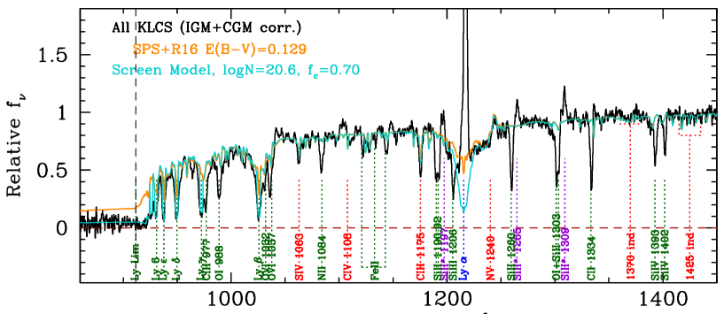
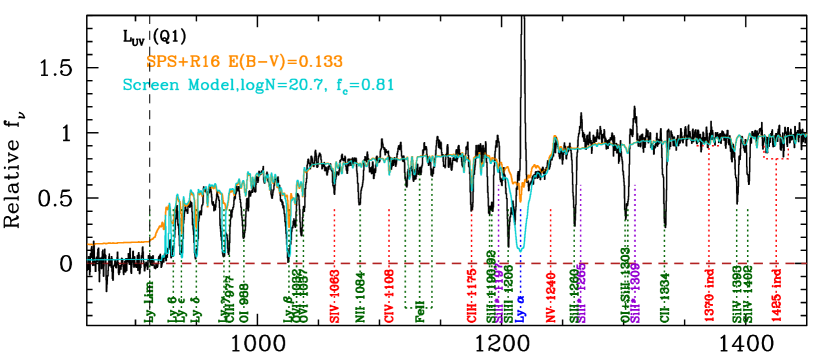
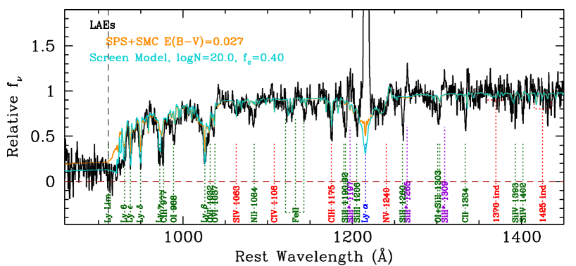
Figure 22.— Example fits using the “screen” model for the galaxy ISM, which includes H I absorption with column density ${\rm log(N_{\rm HI}/cm^{-2})}$ covering a fraction $f_{\rm c}$ of the stellar UV continuum. The values of ${\rm log(N_{\rm HI}/cm^{-2})}$ and $f_{\rm c}$ (see Table 9) are constrained by the damping wings of $\rm Ly\alpha$ and Ly$\beta$  the depth of the higher order Lyman series lines, and the residual LyC flux in the range $\lambda_{0}=880-910$ Å; the model spectrum is otherwise identical to that used for the fits listed in Table 7. Each of the observed spectra (black histograms) has been corrected using the CGM+IGM model appropriate for the source redshift distribution of the galaxies in the sub-sample (thus, adjusted so that $f_{900}/f_{1500}=$$\langle f_{900}/f_{1500}\rangle_{\rm out}$ (see Table 7.)

Using an approach similar to that described by Reddy et al. (2016b), we modeled the ISM for each of the KLCS composite spectra by beginning with the best-fit SPS model (Table 7) and fitting for additional H I line and continuum absorption shortward of $\rm Ly\alpha$. For modeling the Lyman series absorption lines, we assumed a single component with Doppler width $b=125$ km s${}^{-1}\,$, with velocity relative to systemic $v_{\rm sys}=-100$ km s${}^{-1}\,$ (the typical velocity corresponding to the minimum residual flux density of absorption profiles of H I and low-ionization metal lines), and smoothed the artificial line profiles to the resolution of the observed spectra. As described below (see Table 8), only the cores of the first 6 Lyman series lines, the damping wings of $\rm Ly\alpha$ and Ly$\beta$, and the Lyman continuum region ($f_{900}$) were used in evaluating the fits, thus they are insensitive to the precise line profile shapes for saturated lines without damping wings.

Aside from the ISM treatment, the fits are identical to those described in §9.2, where the SPS model is reddened using the attenuation relation that provides the best fit to the CGM+IGM-corrected spectrum in the rest wavelength range 1070-1740 Å, after masking the regions listed in the top portion of Table 8. Simultaneously, we fit for the values of $f_{\rm c}$ and ${\rm log(N_{\rm HI})}$ by comparing the predicted model spectrum with the observed spectrum, where the additional parameters are constrained in the wavelength intervals listed in the bottom part of Table 8. The regions near $\rm Ly\alpha$ (and, to a lesser extent, near Ly$\beta$) are sensitive to H I damping wings for ${\rm log(N_{HI}/cm^{2})\lower 2.15277pt\hbox{$\;\buildrel>\over{\sim}\;$}20.0}$, while the depths of Lyman series lines and the residual LyC emission constrain $f_{\rm c}$. Assuming the same SPS model and attenuation relations used in Table 7, we recorded the values of ${\rm E(B-V)}$, $f_{\rm c}$, and ${\rm log(N_{HI}/cm^{2})}$ that minimized the residuals with respect to the data; these are listed in Table 9. We estimated the uncertainties on each parameter by repeatedly perturbing every pixel of the observed spectrum by an amount consistent with the error spectrum (which includes contributions from both sample variance and shot noise) and refitting. The typical uncertainties on ${\rm E(B-V)}$, $f_{\rm c}$ and ${\rm log(N_{HI}/cm^{2})}$ were found to be $\pm 0.002$, $\pm 0.03$, and $\pm 0.10$, respectively. The best-fit value of $f_{\rm esc,abs}$ computed directly from the models, and the RMS scatter of the best-fit values obtained from repeated fits of the perturbed observed spectra, are listed in the last column of Table 9. Example fits for the full KLCS galaxy sample (“All”), the highest $L_{\rm uv}$ quartile (LQ1), and the subset with $W_{\lambda}(\rm Ly\alpha)>20$ Å (LAEs), are shown in Figure 22.

As noted by Reddy et al. (2016b), $f_{\rm c}$ and $N_{\rm HI}$ generally have little covariance because one ($f_{\rm c}$) is determined by the minima at the cores of Ly series lines and the LyC region, while ${\rm log}N_{\rm HI}$ is constrained by the broad damping wings of $\rm Ly\alpha$. However, as discussed above, column densities in the range ${\rm 18\lower 2.15277pt\hbox{$\;\buildrel<\over{\sim}\;$}log(N_{HI}/cm^{-2})\lower 2.15277pt\hbox{$\;\buildrel<\over{\sim}\;$}20}$ are relatively poorly constrained because there are no discernible $\rm Ly\alpha$ damping wings, yet the resolved Lyman series lines have saturated cores. This affects the fit for the “All, detected” sample, where $f_{\rm c}$ and ${\rm N_{HI}}$ for a fixed $\langle f_{900}/f_{1500}\rangle_{\rm out}$ are less well-determined.

The tabulated $f_{\rm esc,abs}$ values are generally very similar to those listed in Table 7; the difference in the present case is that the fits include constraints provided by the the depth of the Ly series lines and the $\rm Ly\alpha$ damping wings in addition to the measurement of $(f_{900}/f_{1500})_{\rm out}$. Thus, the values listed in Table 9 constitute more stringent checks on the internal consistency of the geometrical model of the ISM: rather than calculating $f_{\rm esc,abs}$ from the SPS fit to the stellar continuum and $(f_{900}/f_{1500})_{\rm obs}$ alone, we now require consistency between the diminution of LyC flux relative to the SPS model and the other observational constraints on the column density and geometric covering fraction of the gas-phase ISM. In this sense, the fits summarized in Table 9 provide additional support for our simplified model for the galaxy ensembles. We return to a discussion of the implications in §10 below.

9.4.2 The “Holes” Model

Table 10ISM Fit Results: Holes Model

Sample	Att	E(B-V)cov	log($N_{\rm HI})$	$f_{\rm c}$	$f_{\rm esc,abs}$
			(${\rm cm}^{-2}$)
All	SMC	0.068	20.57	0.91	$0.09\pm 0.01$
All, detected	SMC	0.085	(17.9)	0.80	$0.31\pm 0.03$
All, not detected	R16	0.163	20.60	0.95	$0.05\pm 0.01$
z(Q1)	SMC	0.076	20.56	0.92	$0.08\pm 0.01$
z(Q4)	R16	0.114	20.34	0.88	$0.12\pm 0.02$
$L_{\rm uv}>L_{\rm uv}^{\ast}$	R16	0.165	20.71	0.96	$<0.04$
$L_{\rm uv}<L_{\rm uv}^{\ast}$	SMC	0.068	20.39	0.87	$0.13\pm 0.03$
$L_{\rm uv}$ (Q1)	R16	0.153	20.64	0.96	$<0.04$
$L_{\rm uv}$ (Q2)	R16	0.195	20.63	0.96	$<0.04$
$L_{\rm uv}$ (Q3)	SMC	0.065	20.39	0.87	$0.13\pm 0.03$
$L_{\rm uv}$ (Q4)	SMC	0.069	20.44	0.84	$0.16\pm 0.03$
$W_{\lambda}(\rm Ly\alpha)$ (Q1)	R16	0.182	21.05	0.97	$<0.03$
$W_{\lambda}(\rm Ly\alpha)$ (Q2)	R16	0.208	20.74	0.97	$<0.04$
$W_{\lambda}(\rm Ly\alpha)$ (Q3)	SMC	0.059	19.93	0.93	$0.07\pm 0.02$
$W_{\lambda}(\rm Ly\alpha)$ (Q4)	SMC	0.054	20.05	0.73	$0.27\pm 0.02$
LAEs	SMC	0.058	20.05	0.71	$0.29\pm 0.03$
non-LAEs	R16	0.174	20.66	0.96	$0.04\pm 0.02$
$W_{\lambda}(\rm Ly\alpha)>0$	SMC	0.059	20.11	0.86	$0.14\pm 0.02$
$W_{\lambda}(\rm Ly\alpha)<0$	R16	0.193	20.97	0.97	$<0.03$
$(G-{\cal R})_{0}$ (Q1)	SMC	0.019	20.28	0.85	$0.15\pm 0.02$
$(G-{\cal R})_{0}$ (Q2)	R16	0.142	20.52	0.94	$0.06\pm 0.02$
$(G-{\cal R})_{0}$ (Q3)	R16	0.195	20.56	0.95	$<0.08$
$(G-{\cal R})_{0}$ (Q4)	R16	0.296	20.87	0.97	$<0.06$

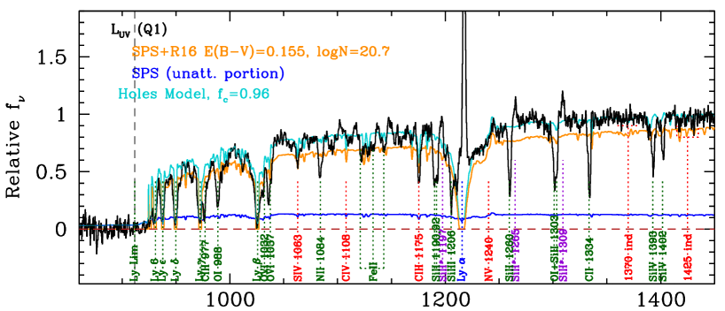
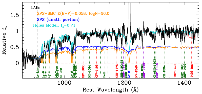
Figure 23.— Fits to the same observed spectra as in Figure 22, but using “holes” models for the galaxy ISM. The model spectra in this case are linear combinations of a component which escapes the galaxy without attenuation (with relative amplitude $1-f_{\rm c}$; blue) and a component (orange) that is both reddened by dust and subject to line and continuum opacity due to H I; the attenuated component has an initial (unabsorbed) relative amplitude $f_{\rm c}$. For this type of model (see Table 10), since the reddened portion of the spectrum must pass through gas with large $N_{\rm HI}$ (with $\tau_{\rm LyC}\lower 2.15277pt\hbox{$\;\buildrel>\over{\sim}\;$}1000$ for typical values of ${\rm log~{}N_{\rm HI}}$), $f_{\rm esc,abs}\simeq(1-f_{\rm c})$.

An alternative model for the effect of the galaxy ISM on the far-UV spectrum is one in which leaking LyC photons escape via completely transparent “holes” in the ISM, as discussed by Reddy et al. (2016b) (see also Zackrisson et al. 2013). This type of model is qualitatively supported by the fact that the equivalent widths of interstellar lines of low-ionization species are correlated with inferred reddening by dust, but the same is not true for higher ionization species like C IV (e.g., Shapley et al. 2003.) In the “Holes” model the spectrum is decomposed into two distinct components, one of which is reddened and absorbed by foreground dust and gas, and the other unattenuated and unabsorbed – and is therefore a scaled version of the intrinsic SPS spectrum. The parameter $f_{\rm c}$ is the fraction of the intrinsic stellar spectrum covered by optically-thick absorbing material along our line of sight, and the net observed spectrum is given by the linear combination

$$S_{\nu,{\rm obs}}=S_{\nu,{\rm int}}\left[(1-f_{\rm c})+f_{\rm c}~{}{\rm e^{-\tau(\lambda)}}10^{-A_{\lambda}/2.5}\right]$$ (17)

where $A_{\lambda}=k_{\lambda}E(B-V)_{\rm cov}$ and $E(B-V)_{\rm cov}$ is the reddening applied to the covered portion of the galaxy The second term on the righthand side of equation 17 also accounts for H I line and continuum opacity as described in the previous section. For each KLCS composite spectrum, we fitted for the model values of $f_{\rm c}$, ${\rm log(N_{\rm HI}/cm^{-2})}$, and $E(B-V)_{\rm cov}$ that minimized $\chi^{2}$; the best-fit model parameters are given in Table 10. Figure 23 shows the decomposition of the best fitting holes models for the same composites shown in Figure 22.

The main difference between the screen and holes models is the interpretation of $f_{\rm c}$: for the holes case, the differential attenuation between the covered and uncovered components requires accounting for extinction as part of the calculation of $f_{\rm c}$; this is easily seen in the top panel of Figure 23, which shows that the relative contributions of the attenuated and unattenuated components to the observed (non-ionizing) spectrum are in the ratio $\sim 3:1$, while geometrically the ratio is $f_{\rm c}/(1-f_{\rm c})\sim 10$. The concept $f_{\rm esc,rel}$ is probably less useful in the context of the holes models, since $\langle f_{900}/f_{1500}\rangle_{\rm out}$ now has a more complex relationship to the intrinsic SED of the SPS spectrum than in the screen case (because of the assumption of two independent components, one affected by dust and the other unaffected.)

However, in the holes models, $f_{\rm esc,abs}$ is very straightforward to estimate provided $\tau(\rm{LyC})\gg 1$ for the covered component, in which case

$$f_{\rm esc,abs}\simeq 1-f_{\rm c}~{}.$$ (18)

Equation 18 applies to all of the models listed in Table 10 except for the composite of individually-detected galaxies (“All, detected”). As discussed previously, the appropriate CGM+IGM correction for this sub-sample is much more uncertain than for any of the other composites; with the assumptions adopted earlier – that the detected subsample has IGM+CGM transmission drawn from the highest 12% – the best-fit model spectrum has $1-f_{\rm c}\approx 0.20$ but $f_{\rm esc,abs}$ has an additional contribution from ionizing photons that have passed through the H I layer without being completely attenuated (because the LyC optical depth is of order unity).

9.5. Model Assessment

Models fits for both the screen and the holes models can simultaneously reproduce the overall spectral shape, the depth of the Lyman series absorption lines, the wings of the interstellar $\rm Ly\alpha$ absorption feature, and the residual LyC flux using the same underlying SPS model. There is a slight tendency for both sets of ISM models to over-estimate the residual LyC flux for composites having the lowest values of $\langle f_{900}/f_{1500}\rangle_{\rm out}$ : e.g., the $L_{\rm uv}>L_{\rm uv}^{\ast}$ sub-sample has $\langle f_{900}/f_{1500}\rangle_{\rm out}$$=0.006\pm 0.008$ (Table 6) but the best-fit model gives $\langle f_{900}/f_{1500}\rangle_{\rm out}$$\sim 0.03$ (Tables 9 and 10). Such discrepancies would be expected if the covering fraction of the optically thick ISM layer is slightly underestimated by the cores of the Lyman series lines, or if there is H I with $17.5\lower 2.15277pt\hbox{$\;\buildrel<\over{\sim}\;$}{\rm log(N_{HI}/cm^{2})}\lower 2.15277pt\hbox{$\;\buildrel<\over{\sim}\;$}20$ that does not contribute significantly to the $\rm Ly\alpha$ damping wings and whose Lyman series lines are not fully resolved in the spectra (and thus their depth is underestimated). Since the parameter $f_{\rm c}$ is constrained in our modeling by simultaneously matching the LyC residuals (which should not depend on spectral resolution) and the Lyman series line depths (which may depend on resolution), larger reduced $\chi^{2}$ evaluated over those spectral regions would flag inconsistencies.

Another possibility of course is that $\langle f_{900}/f_{1500}\rangle_{\rm out}$ is underestimated due to residual systematics in the background subtraction, in this case over-subtraction; this possibility cannot be ruled out entirely, but seems less likely than the presence of unresolved intermediate column density H I.

Broadly speaking, the success of the simple models presented above demonstrates that there are real trends within the KLCS sample among the depth of the Lyman series lines, the residual LyC flux, and the column density of the dominant component of ISM $N_{\rm HI}$ absorption; the trends – increased LyC leakage in galaxies with lower $N_{\rm HI}$, lower inferred $f_{\rm c}$, and larger $W_{\lambda}(\rm Ly\alpha)$ – are in the direction one might have anticipated. We consider a simple physical interpretation of the results in §11.1, where we conclude that the “Holes” model does surprisingly well in explaining the observed interconnections between the observable quantities.

10. Implications of Escape Fraction Results

The term “escape fraction” has come to represent several different quantities, depending on the context and the underlying assumptions. We have gone through the exercise in the previous sections of calculating a number of different quantities related to LyC escape, justifying underlying assumptions by demonstrating that they do not lead to internal inconsistencies. Here we briefly digress to review the different quantities and the extent to which they are model- or assumption-dependent. As above, we begin with the most model-independent quantities, and proceed in order of increasing model dependence:

10.1. $\langle f_{900}/f_{1500}\rangle_{\rm obs}$

Assuming that the observations are free of systematics that would invalidate the results, this quantity is entirely model-independent; however, it is of only limited use for individual objects because it is so strongly modulated by the variations of CGM+IGM opacity among different lines of sight (§7). With ensembles in which more than $\simeq 30$ objects with similar redshifts and common observed properties are considered, the mean value of $(f_{900}/f_{1500})_{\rm obs}$ can be corrected using empirically-calibrated IGM+CGM models to obtain $\langle f_{900}/f_{1500}\rangle_{\rm out}$. For the KLCS sample, $0\leq\langle f_{900}/f_{1500}\rangle_{\rm obs}\leq 0.14$ among the galaxy subsamples (Table 6), with a sample mean of $\langle f_{900}/f_{1500}\rangle_{\rm obs}=0.021\pm 0.002$.

10.2. $\langle f_{900}/f_{1500}\rangle_{\rm out}$

This parameter is the most important one, in practical terms, for estimating the contribution of a galaxy population of known far-UV (e.g., at rest-frame 1500 Å) luminosity function to the metagalactic ionizing radiation field (see §11.4.) By our definition, this ratio characterizes the flux density of ionizing photons averaged over the 880-910 Å window, relative to the non-ionizing UV flux density near 1500 Å, statistically corrected for IGM+CGM opacity back to the “galaxy photosphere” at $r_{\rm gal}=50$ kpc. As discussed in §7, the statistical uncertainty on the IGM correction is drastically reduced for an ensemble of galaxies provided the lines of sight are independent and the sample selection does not depend significantly on the IGM properties at fixed redshift. Remaining systematic uncertainties in the values of $\langle t_{900}\rangle$ for an ensemble will stem primarily from the treatment of the CGM and possible systematic differences in the large-scale IGM environment.

Table 6 includes values of $\langle t_{900}\rangle$ under two different assumptions for the H I column density distribution for distances $r>50$ pkpc from a galaxy; $\langle t_{900}\rangle$ values with and without an enhancement in $N_{\rm HI}$ from the CGM typically differ by $\sim 20$%, which likely over-estimates the true level of systematic uncertainty, but would be a conservative upper limit. As Table 6 indicates, such systematics, if present, would affect the inferred values of $f_{\rm esc,rel}$ and $f_{\rm esc,abs}$ by a similar factor.

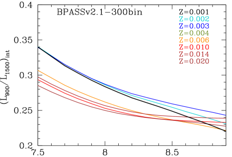
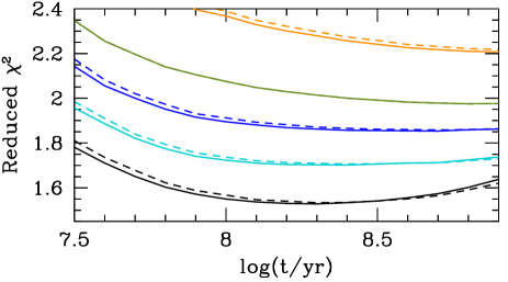
Figure 24.— (Top:) Model predictions for the intrinsic flux density ratio $(L_{900}/L_{1500})_{\rm int}$ for BPASSv2.1-300bin-IMF135 continuous star formation models (Eldridge et al. 2017) evaluated as a function of assumed age and stellar metallicity; the latter varies from $Z_{\ast}=0.001$ ($\sim 0.07Z_{\odot}$) to $Z_{\ast}=0.020$ ($\sim 1.4Z_{\odot}$), or $-1.15\leq{\rm[Fe/H]}\leq+0.15$. (Bottom:) Relative values of $\chi^{2}/\nu$ for models versus age, color-coded according to stellar metallicity as in the top panel, for the best-fitting model relative to the full KLCS composite spectrum (“All”). The solid curves correspond to the “screen” models, and the dashed curves to the “holes” models. The $Z=0.001$ models provide by far the best fits at all ages; the best-fitting $Z=0.001$ models have ${\rm log(t/yr)\simeq 8.2-8.3}$ ($\simeq 160-200$ Myr).

10.3. $\langle f_{\rm esc,rel}\rangle$

As discussed in §9.1 above, $f_{\rm esc,rel}$ is a useful concept if the intrinsic $(L_{900}/L_{1500})_{\rm int}$ of a galaxy’s integrated stellar population is known, since the latter ratio is the absolute maximum possible $(f_{900}/f_{1500})_{\rm out}$; i.e., $f_{\rm esc,rel}$ approaches unity only when there is no H I with appreciable LyC optical depth between the observed stars and $r_{\rm gal}\sim 50$ pkpc.

If $f_{\rm esc,rel}\leq 1$, $(L_{900}/L_{1500})_{\rm int}\simeq 0.28$ (§9.2; Figure 24), and $\langle t_{900}\rangle\simeq 0.37$ (Table 6), then the maximum value of $\langle f_{900}/f_{1500}\rangle_{\rm obs}$ expected for an ensemble of galaxies with $z_{\rm s}\simeq 3.05$ is $\langle f_{900}/f_{1500}\rangle_{\rm obs,max}\simeq 0.11$. For an individual galaxy with $z_{\rm s}=3.05$, $t_{900}<0.67$ (the $\sim 99$th percentile IGM+CGM transmission; see Table 12), $(f_{900}/f_{1500})_{\rm obs,max}\simeq 0.30\times 0.67\simeq 0.20$. Accounting for dust or assuming a more typical IGM sightline would immediately reduce the expected upper limits on observed values. These small numbers would be reduced by large factors if the LyC regions were not sampled optimally (§7.2), or the source redshift were significantly higher (§7). A corollary to these considerations is that one should be suspicious of individual measurements of LyC leakage if $(f_{900}/f_{1500})_{\rm obs}\lower 2.15277pt\hbox{$\;\buildrel>\over{\sim}\;$}0.2$, and of ensemble measurements with $\langle f_{900}/f_{1500}\rangle_{\rm obs}\lower 2.15277pt\hbox{$\;\buildrel>\over{\sim}\;$}0.11$.

Clearly, assuming a different SPS model, with a different $(L_{900}/L_{1500})_{\rm int}$, would also change the inferred $f_{\rm esc,rel}$ given a measurement of, or limit on, $(f_{900}/f_{1500})_{\rm out}$. Figure 24 shows the metallicity and age dependence of $(L_{900}/L_{1500})_{\rm int}$ (including self-consistently the contribution of nebular continuum emission to the non-ionizing UV light) for constant SFR BPASSv2.1-300bin models. In the context of such models, typical $z\sim 3$ galaxies have SED-inferred ages of $\sim 50-500$ Myr (${\rm 7.7\lower 2.15277pt\hbox{$\;\buildrel<\over{\sim}\;$}log(t/yr)\lower 2.15277pt\hbox{$\;\buildrel<\over{\sim}\;$}8.7}$); the $Z=0.001$ model that best reproduces the details of the observed spectra has $0.24\lower 2.15277pt\hbox{$\;\buildrel<\over{\sim}\;$}(L_{900}/L_{1500})_{\rm int}\lower 2.15277pt\hbox{$\;\buildrel<\over{\sim}\;$}0.33$ over the same age range. Assuming younger ages for the SPS models would, naively, lower the required value of $f_{\rm esc,abs}$ to match an observed $(f_{900}/f_{1500})_{\rm out}$; however, younger SPS models are somewhat bluer in the non-ionizing FUV, so that matching an observed galaxy SED requires more reddening by dust – and all reasonable dust attenuation relations have $k_{\lambda}(900)>k_{\lambda}(1500)$, meaning that additional reddening reduces $f_{900}$ relative to $f_{1500}$. For the screen models, fits of BPASSv2.1 models to the full KLCS galaxy composite with the same IMF and stellar metallicity ($Z_{\ast}=0.001$) but varying the age over the range ${\rm log(t/yr)=[7.5\rightarrow 9.0]}$ results in monotonic variation in best-fit parameter values: $E(B-V)$ [$0.145\rightarrow 0.085$], C1500 [$3.29\rightarrow 2.01$], $N_{\rm HI}$ [$20.80\rightarrow 20.05$], and $f_{\rm esc,abs}$ [$0.097\rightarrow 0.191$], but only small changes in $f_{\rm esc,rel}$ [$0.32\rightarrow 0.38$] and $f_{\rm c}$ [$0.73\rightarrow 0.68$]. However, the best fits to the spectra– both in terms of reproducing the details of the stellar continuum and matching the observed LyC residuals, Lyman series line depths, and $\rm Ly\alpha$ damping wings – are obtained for ${\rm 7.9\lower 2.15277pt\hbox{$\;\buildrel<\over{\sim}\;$}log(t/yr)\lower 2.15277pt\hbox{$\;\buildrel<\over{\sim}\;$}8.5}$, where the parameters are consistent with those listed in Table 9 for the fiducial ${\rm log(t/yr)=8.0}$ model (see the bottom panel of Figure 24.)

10.4. $f_{\rm esc,abs}$

In this section we have tried to emphasize that the parameter often seen as the “holy grail” of LyC studies – the absolute escape fraction $f_{\rm esc,abs}$ – is several steps removed from an observational measurement, even at $z\sim 3$ where direct measurements of residual LyC emission are feasible. Each of the steps is model-dependent, beginning with uncertainty in the shape and absolute intensity of the unattenuated EUV and FUV light from stars, followed by the net effect of dust on both the ionizing and non-ionizing UV, and, finally, the rather poorly-defined notion of what constitutes “escape” of an ionizing photon from the galaxy in which it was produced.

However, we have also attempted to leverage recent progress in understanding the ionizing sources through joint analysis of the stellar and nebular spectra (e.g., Steidel et al. 2016; Strom et al. 2017) and to follow a self-consistent thread capable of reconciling the detectability of LyC radiation leakage with all other available empirical constraints. With these caveats, we have measured $f_{\rm esc,abs}$ for a sample of $\simeq L_{\rm uv}^{\ast}$ galaxies at $z\sim 3$. Focusing on the “holes” models, for reasons discussed in more detail in the next section, the bottom line is that some galaxies appear to leak a substantial fraction of the ionizing radiation they produce– up to 30% for those in the highest quartile of $W_{\lambda}(\rm Ly\alpha)$, while others - notably the brightest galaxies, and those which have $\rm Ly\alpha$ strongly in absorption – leak at most imperceptibly ($<3$% at 2$\sigma$.) Averaged over the KLCS sample, all of which has $L_{\rm uv}$ within a factor of a few of $L_{\rm uv}^{\ast}$ at $z\sim 3$, $\langle f_{\rm esc,abs}\rangle\sim 9$% given our assumed SPS and reddening models (Table 10).

It is important to keep in mind the degree to which $f_{\rm esc,abs}$ depends on the latter assumptions – if, for example, we had assumed that the attenuation relation is that of Calzetti et al. (2000) and that the appropriate SPS model is a solar-metallicity Starburst99 model (Leitherer et al. 2014; see Steidel et al. 2016 for comparisons with the BPASSv2.0 models), then the best-fitting model parameters give $f_{\rm esc,abs}=0.25$, a factor of more than two times higher than our fiducial model (Table 7), but still under-predict the observed LyC flux by a factor of $\lower 2.15277pt\hbox{$\;\buildrel>\over{\sim}\;$}3$. Changing the attenuation relation to R16 but keeping the SPS model fixed, $f_{\rm esc,abs}=0.33$, with similarly poor $\chi^{2}$ relative to the observed spectrum (Figure 24.) With the wrong choice of SPS model, it is not possible to simultaneously match the shape of the FUV spectrum, the Lyman series line depth, and the residual LyC emission (see also Reddy et al. 2016b.)

10.5. Comparison to Other Recent Results

10.5.1 High Redshift

Given the many quantities commonly used to describe LyC measurements, it is useful to compare our results to others from the recent literature. The most directly comparable, in that the results involve composite spectral stacks, have been discussed by Marchi et al. 2017a, b, using spectra obtained as part of the VUDS Survey (Le Fèvre et al. 2015). Due to the minimum wavelength of $\simeq 3800$ Å the samples include only galaxies having $3.5\leq z_{\rm s}\leq 4.3$ (median $z_{\rm s}=3.8$.)

Marchi et al. (2017a) use a sample of 33 galaxies which were conservatively culled from an original sample of 46 using multi-band HST imaging to eliminate any significant possibility of foreground contamination. Their spectral stack, using a weighted average, has $\langle f_{900}/f_{1500}\rangle_{\rm obs}=0.008\pm 0.004$ at median redshift $\langle z\rangle=3.80$. If we apply our own determination of the mean IGM+CGM transmission at $z\simeq 3.8$, $\langle t_{900}\rangle\simeq 0.25$ ($\simeq 10$% lower than the transmission assumed by Marchi et al. 2017a) to facilitate a direct direct comparison with LLS, one obtains $\mbox{$\langle f_{900}/f_{1500}\rangle_{\rm out}$}\simeq 0.032\pm 0.016$, somewhat smaller than that of the full KLCS sample ($\mbox{$\langle f_{900}/f_{1500}\rangle_{\rm out}$}=0057\pm 0.006$; Table 6.). However, the Marchi et al. (2017a) sample is on average $\simeq 1$ magnitude brighter (in terms of $M_{\rm uv}$) than KLCS; in addition, only 12 of 33 galaxies (36%) have $\rm Ly\alpha$ appearing in emission, compared with 74/124 (60%) in the KLCS sample, in spite of the significantly higher mean redshift of the former. As discussed above, the KLCS results would predict that a brighter sample, dominated by galaxies with $\rm Ly\alpha$ observed in absorption, would have relatively low $\langle f_{900}/f_{1500}\rangle_{\rm out}$ (see Table 6.)

Marchi et al. (2017b) use a different subset of VUDS to investigate the dependence of $\langle f_{900}/f_{1500}\rangle_{\rm out}$ on properties believed to be correlated with LyC leakage based on existing detections at low and high redshift. They conclude that galaxies with large $W_{\lambda}(\rm Ly\alpha)$ and compact physical sizes (in the UV continuum and/or in $\rm Ly\alpha$ emission) show evidence for significantly higher $\langle f_{900}/f_{1500}\rangle_{\rm out}$ than the remainder of the sample. Again adopting the measurements of $\langle f_{900}/f_{1500}\rangle_{\rm obs}$ and applying our estimated mean IGM+CGM transmission at $z\simeq 3.8$ for consistency, we find that the subsample with $W_{\lambda}(\rm Ly\alpha)>50$ Å has $\mbox{$\langle f_{900}/f_{1500}\rangle_{\rm out}$}\simeq 0.3$, a factor of $\simeq 2$ higher than the KLCS subsamples with the largest $\langle f_{900}/f_{1500}\rangle_{\rm out}$ measured at $z=3.05$. However, all subsets of the $\langle z_{\rm s}\rangle=3.8$ spectra imply $\mbox{$\langle f_{900}/f_{1500}\rangle_{\rm out}$}\lower 2.15277pt\hbox{$\;\buildrel>\over{\sim}\;$}0.17$, and the authors are careful not to claim to have measured uncontaminated values of $\langle f_{900}/f_{1500}\rangle_{\rm out}$. In fact, if one adopts lowest-measured $\langle f_{900}/f_{1500}\rangle_{\rm out}$ as the zero point, the differential between their highest and lowest $\langle f_{900}/f_{1500}\rangle_{\rm out}$ subsamples would yield $\mbox{$\langle f_{900}/f_{1500}\rangle_{\rm out}$}\simeq 0.16$, entirely consistent with the maximum $\langle f_{900}/f_{1500}\rangle_{\rm out}$ among the KLCS sub-samples (Table 6.). Thus, we conclude that the results of both studies are consistent with those of KLCS.

10.5.2 Low Redshift

As mentioned in §1, several recent programs targeting analogs of high redshift galaxies have successfully detected LyC emission from low-redshift ($z\simeq 0.3$) galaxies using HST/COS The highest success rate, and the largest values of $\langle f_{\rm esc,abs}\rangle$, have been measured for galaxies selected on the basis of unusually high values of the strong emission line index [O III]$\lambda\lambda 4960$,5008/[O II]$\lambda\lambda 3727$,3729$\equiv$O32 (Izotov et al. 2016a, b.) The rationale behind the selection is that high O32 may indicate the presence of density-bounded H II regions signifying local escape of significant LyC emission. (Jaskot & Oey 2013; Nakajima & Ouchi 2014). Of five objects with ${\rm O32}>4$, all 5 are LyC detections , with $\mbox{$\langle f_{\rm esc,abs}\rangle$}=0.06-0.13$, similar to the mean value for the KLCS sample. Subsequently, a more extreme low-redshift galaxy with ${\rm O32=11.5}$ and $\mbox{$\langle f_{\rm esc,abs}\rangle$}=0.46$, has been identified by Izotov et al. (2018), comparable to $\langle f_{\rm esc,abs}\rangle$ estimated for the directly detected sub-sample of KLCS (Table 10.) The $\rm Ly\alpha$ properties of the O32-selected low-z galaxies (Verhamme et al. 2017; Izotov et al. 2018), also found to be unusual, are discussed in §11.2.1 below.

11. A Model for Lyman Continuum Escape

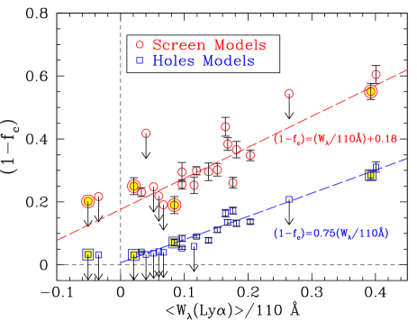
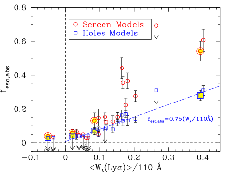
Figure 25.— (Left:) The best-fit value (see Tables 9 and 10) (1-$f_{\rm c}$) for each of the composite spectra, where $f_{\rm c}$ is the inferred fraction of the stellar continuum covered by optically thick H I based on the joint constraints provided by the depth of the Lyman series absorption and the residual LyC emission ($\langle f_{900}/f_{1500}\rangle_{\rm out}$). (Right:) As for the lefthand panel, where (1-$f_{\rm c}$) has been replaced by $f_{\rm esc,abs}$ under the Screen and Holes models. Note that, because of the way $f_{c}$ is defined for Holes models, (1-$f_{\rm c}$) is essentially identical to $f_{\rm esc,abs}$ except for the ”All, Detected” subsample. The points representing the 4 independent quartiles in $W_{\lambda}(\rm Ly\alpha)$ are highlighted with lightly-shaded larger symbols.

11.1. Trends with $W_{\lambda}(\rm Ly\alpha)$

In §8, we observed a strong dependence of the residual LyC emissivity $\langle f_{900}/f_{1500}\rangle_{\rm out}$ on spectroscopically-measured $W_{\lambda}(\rm Ly\alpha)$, and noted (Figure 17) that the relation could be captured approximately by a linear relation

$${\rm\mbox{$\langle f_{900}/f_{1500}\rangle_{\rm out}$}\simeq 0.36\left[\frac{\langle W_{\lambda}(\rm Ly\alpha)\rangle}{110~{}\textrm{\AA}}\right]+0.02}$$ (19)

The parametrization of equation 19 was chosen in part because the fiducial BPASSv2.1-300bin-t8.0 continuous star formation models used to fit the sub-sample composite spectra in §9.4.1 and §9.4.2 predict that $W_{\lambda}(\rm Ly\alpha)\simeq 110$ Å, assuming “Case B” (ionization bounded) recombination and no selective attenuation of $\rm Ly\alpha$ photons relative to the FUV continuum near $\rm Ly\alpha$. The term inside square brackets is therefore the ratio of observed $W_{\lambda}(\rm Ly\alpha)$ to the maximum value expected under the most favorable conditions for $\rm Ly\alpha$ production, i.e., where every LyC photon has been absorbed and converted to $\rm Ly\alpha$ or nebular continuum in accordance with Case B expectations. An observation of the maximum $W_{\lambda}(\rm Ly\alpha)$ would also require that, within the spectroscopic aperture, the intensity of the $\rm Ly\alpha$ emission line relative to the continuum flux density has not been significantly altered by resonant scattering of $\rm Ly\alpha$ (i.e, spatial redistribution and/or selective absorption of $\rm Ly\alpha$ photons by dust grains; see, e.g., Steidel et al. 2011).

The lefthand panel of Figure 25 illustrates the nearly-linear relationship between $1-f_{\rm c}$ (Tables 9 and 10 for the Screen and Holes models, respectively) and $\langle W_{\lambda}(\rm Ly\alpha)\rangle$ among the composite spectra. This behavior strongly supports the hypothesis of a direct causal link between $W_{\lambda}(\rm Ly\alpha)$ in emission and the depth/strength of interstellar absorption features observed in the same galaxy spectra (e.g., Shapley et al. 2003; Steidel et al. 2010, 2011; Jones et al. 2012); it also lends credence to the use of simple geometric models of the galaxy ISM to understand the interplay between residual LyC emission, the depth of Lyman series absorption lines, and $\rm Ly\alpha$ escape. The sense of the relationship is that the fraction of the Case B $W_{\lambda}(\rm Ly\alpha)$ (110 Å in our model) measured within a spectroscopic aperture is directly related to the portion of the stellar UV continuum that is not covered by optically-thick H I ($1-f_{\rm c}$) along the same line of sight.

Of course, one does not expect the production rate of $\rm Ly\alpha$ photons to be compatible with Case B assumptions if there is significant detection of residual LyC flux, since any detected ionizing photons will not have produced the corresponding $\rm Ly\alpha$ photons expected for an ionization-bounded geometry. For a typical value $1-f_{\rm c}\simeq 0.1$, the reduction in the $\rm Ly\alpha$ source function would be small; however, in the limit of very high $1-f_{\rm c}\sim 1$, an observer would see $\rm Ly\alpha$ emission along the same line of sight only if the photons have been scattered in our direction after (initially) being emitted in another. In all likelihood this suggests that the correlation between $(1-f_{\rm c})$ or $f_{\rm esc,abs}$ and $W_{\lambda}(\rm Ly\alpha)$ would turn over $f_{\rm esc,abs}\lower 2.15277pt\hbox{$\;\buildrel>\over{\sim}\;$}0.5$. Conversely, galaxies with $W_{\lambda}(\rm Ly\alpha)\sim W_{\lambda}(\rm Ly\alpha,{\rm CaseB})\simeq 110$Å are a priori unlikely to exhibit substantial LyC leakage.

In other words, equation 19 should not be extrapolated beyond the range covered by the KLCS composites, which all have $\langle W_{\lambda}(\rm Ly\alpha)\ \rangle<50$ Å; only 6 individual KLCS sources have spectroscopically measured $W_{\lambda}(\rm Ly\alpha)>50$ Å  and only one has $W_{\lambda}(\rm Ly\alpha)>100$ Å (see Table 2).

The relationships shown in Figure 25 are surprisingly tight, given the complexity of $\rm Ly\alpha$ radiative transfer compared to that of ionizing photons; for example, $\rm Ly\alpha$ can be scattered by H I with $N_{\rm HI}$$\ll 10^{17}$ cm^-2, and $\rm Ly\alpha$ resonant scattering may increase the probability of absorption by dust or of scattering into a diffuse $\rm Ly\alpha$ halo, in which case an aperture tailored to the apparent angular scale of the FUV continuum light (as for KLCS spectra) might miss a large fraction of the emergent $\rm Ly\alpha$ flux (see, e.g., Steidel et al. 2011; Hayes et al. 2014; Wisotzki et al. 2016). However, a “down the barrel” spectrum which includes a LyC detection will also capture the fraction of $\rm Ly\alpha$ photons that pass through the same low optical depth holes in the ISM. The tightness of the relationships shown in Figure 25 suggests that most $\rm Ly\alpha$ photons detected within the spectroscopic aperture may have passed through the same holes in the ISM. This scenario is easier to explain in the context of the “holes” models, as shown by the small scatter in both panels of Figure 25 – evidently, applying dust attenuation to the entire EUV/FUV continuum makes it more difficult to account for the tightness of the correlation between $\langle f_{900}/f_{1500}\rangle_{\rm out}$ and $W_{\lambda}(\rm Ly\alpha)$. We also expect that using a larger aperture to measure the same galaxies would increase the scatter between $W_{\lambda}(\rm Ly\alpha)$ and $\langle f_{900}/f_{1500}\rangle_{\rm out}$ as an increasing fraction of the observed $\rm Ly\alpha$ photons will have been scattered to large galactocentric radii via less direct channels through the ISM than the LyC photons.

In the discussion that follows, we continue to adopt the “holes” model as the simplest picture that remains consistent with the current observations.

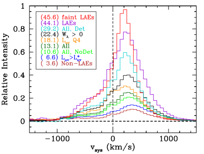
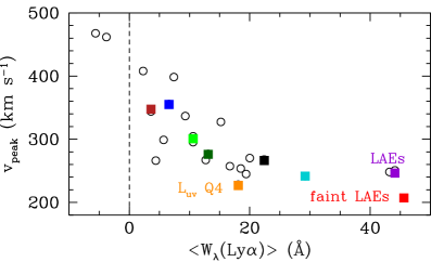
Figure 26.— (Top:) Stellar continuum subtracted $\rm Ly\alpha$ emission line intensity profiles (i.e., the area under the profile is proportional to $W_{\lambda}(\rm Ly\alpha)$) for selected KLCS sub-samples. The profiles are color-coded according to the legend, which also includes the value of $W_{\lambda}(\rm Ly\alpha)$/Å as given in Table 6. The spectrum labeled “faint LAEs” is the stacked profile of 300 continuum-faint $\rm Ly\alpha$-selected LAEs at $z\sim 2.7$ from Trainor et al. (2015) with $M_{\rm uv}\sim-18$ (i.e., $\sim 10$ times fainter than the LAEs in the KLCS sample). (Center:) The systemic velocity of the red peak of $\rm Ly\alpha$ emission, $v_{\rm peak}$, color-coded as in the legend for the top panel. Although $W_{\lambda}(\rm Ly\alpha)$ varies by a factor of $\sim 15$ and $v_{\rm peak}$ is clearly correlated with $\langle W_{\lambda}(\rm Ly\alpha)\rangle$, the fraction of the total $\rm Ly\alpha$ emission with $v<0$ is remarkably constant among all of the composite profiles: $f(\rm Ly\alpha,{\rm blue})=0.31\pm 0.02$. (Bottom:) As in the center panel, but with the measured values of $\langle W_{\lambda}(\rm Ly\alpha)\rangle$ replaced by the inferred $\langle f_{\rm esc,abs}\rangle$.

11.2. $\rm Ly\alpha$ Emission Line Kinematics

Theoretical predictions concerning the relationship between the kinematics and escape of $\rm Ly\alpha$ emission and the leakage of significant LyC emission have varied depending on the physical model assumed for the structure and kinematics of the ISM (e.g., Yajima et al. 2014; Verhamme et al. 2015; Dijkstra et al. 2016; Verhamme et al. 2017). In general, most models predict that if the ISM is porous enough to allow the escape of ionizing photons along a particular line of sight, then one should also observe $\rm Ly\alpha$ emission with a significant component near $v_{\rm sys}\simeq 0$ and/or a double-peaked profile with small velocity separation, which might indicate relatively low $N_{\rm HI}$ along the line of sight. However, the picture that seems indicated by the KLCS results is that, while there is an overall correlation between the inferred value of $N_{\rm HI}$ associated with the covered portion of the stellar continuum and $f_{\rm esc,abs}$ (see, e.g., Table 10), it is the covering fraction ($f_{\rm c}$) that appears most closely linked with LyC leakage (as well as with $W_{\lambda}(\rm Ly\alpha)$). Since the measured values of $N_{\rm HI}$ are far too high to have allowed any detectable LyC leakage if the entire stellar UV continuum were covered, the apparent connection between $N_{\rm HI}$ and $\langle f_{\rm esc,abs}\rangle$ may simply indicate that the incidence of clear channels through the ISM is higher when the characteristic $N_{\rm HI}$ (with covering fraction $f_{\rm c}$) is lower. Similar results have recently been obtained for a sample of LyC-detected low-redshift galaxies with $N_{\rm HI}$ measurements (Gazagnes et al. 2018; Chisholm et al. 2018).

Interestingly, among the KLCS subsample composites, none exhibits a $\rm Ly\alpha$ peak near $v\sim 0$ – including the composite formed entirely of individual LyC detections – as shown in Figure 26. Indeed, the overall shapes of the $\rm Ly\alpha$ profiles – including the subsample comprised of individual LyC detections – are remarkably similar, with a fraction $f(\rm Ly\alpha,{\rm blue})\simeq 0.31\pm 0.02$ of the total $\rm Ly\alpha$ emission emerging with $v_{\rm sys}<0$. The center panel of Figure 26 shows that the velocity relative to systemic of the $\rm Ly\alpha$ red peak ($v_{\rm peak}$) decreases with increasing $\langle W_{\lambda}(\rm Ly\alpha)\rangle$, as found by Erb et al. (2014); Trainor et al. (2015) for similar-sized samples of LBGs and LAEs at $z\sim 2-3$. Nevertheless, the bottom panel of Figure 26) shows that the KLCS subsamples with $\mbox{$\langle f_{\rm esc,abs}\rangle$}\lower 2.15277pt\hbox{$\;\buildrel>\over{\sim}\;$}0.1$ tend to have a nearly constant $v_{\rm peak}\sim 250$ km s${}^{-1}\,$, whereas those with $\mbox{$\langle f_{\rm esc,abs}\rangle$}\lower 2.15277pt\hbox{$\;\buildrel<\over{\sim}\;$}0.1$ exhibit a wide range in $v_{\rm peak}$. The faint LAE sample of Trainor et al. (2015) (whose LyC properties are unknown, but which have Lyman $\beta$ line depths similar to the KLCS LAE sample) continues a trend of slightly smaller $\rm Ly\alpha$ velocity shifts for intrinsically fainter galaxies at fixed $W_{\lambda}(\rm Ly\alpha)$ (center panel of Figure 26); this, along with the accompanying smaller maximum blueshifted velocity of the low-ionization metals, is attributed to lower outflow velocities. It is therefore quite possible that the characteristic $v_{\rm peak}$ at fixed $\langle f_{\rm esc,abs}\rangle$ would also be smaller for galaxies with $M_{\rm uv}>-19.5$.

Clearly, $\rm Ly\alpha$ peaking at $v=0$ is not a necessary condition for significant LyC leakage among galaxies with $z\simeq 3$. The non-zero vales of $v_{\rm peak}$ among LyC-detected subsamples suggests that most $\rm Ly\alpha$ photons escaping along the same line of sight as LyC photons have been scattered at least once from gas moving with $v_{\rm sys}>0$. This suggests that the holes through the ISM allowing LyC photons to escape are not generally optically thin to $\rm Ly\alpha$ photons without the benefit of a velocity kick to move them off resonance of gas near $v_{\rm sys}=0$.

11.2.1 Comparison to Low-Redshift Results

Verhamme et al. (2017) analyze the statistics of $\rm Ly\alpha$ emission among the sample of known LyC emitters at low redshift, and compare them to larger samples of potential analogs to high redshift galaxies, including LBAs (Heckman et al. 2011), Green Peas (GPs; Jaskot & Oey 2014; Henry et al. 2015), and galaxies drawn from the $\rm Ly\alpha$ Reference Sample (LARS; Östlin et al. 2014; Hayes et al. 2014; Rivera-Thorsen et al. 2015.) With the recent addition of the more extreme object J1154+2443 (Izotov et al. 2018), there are 6 high-O32-selected low-z galaxies with LyC detections. All have reported $W_{\lambda}(\rm Ly\alpha)\geq 75$ Å, and, perhaps more significantly, $\rm Ly\alpha$ profiles with no discernible absorption component and relatively small velocity differences between the blueshifted and redshifted peaks of $\rm Ly\alpha$ ($\Delta v_{\rm Ly\alpha}\sim 200-400$ km s${}^{-1}\,$). Verhamme et al. (2017) argue that a small $\Delta v_{\rm Ly\alpha}$ is a model-independent signature of low foreground $N_{\rm HI}$, and therefore a reliable predictor of significant LyC emission. Izotov et al. (2018) further suggests that there is a dependent relationship between $\langle f_{\rm esc,abs}\rangle$ and both O32 and $\Delta v_{\rm Ly\alpha}$. We are currently unable to test the O32 dependence in the KLCS sample, though we note that ${\rm O32}>4$ is satisfied by a substantial fraction ($\simeq 40$%) of $z\sim 3$ galaxies in the KBSS-MOSFIRE sample, which were selected using continuum criteria identical to those of KLCS.

Caution must be used in comparing values of $W_{\lambda}(\rm Ly\alpha)$ between samples, since $W_{\lambda}(\rm Ly\alpha)$ is known to depend on aperture size for both low-z (Hayes et al. 2014) and high-z (Steidel et al. 2011; Wisotzki et al. 2016) galaxies. With this caveat in mind, the O32-selected low-z galaxies have larger $W_{\lambda}(\rm Ly\alpha)$ than any of the KLCS composite sub-samples; two of the individual KLCS galaxies have spectroscopically-measured $W_{\lambda}(\rm Ly\alpha)>75$ Å, both of which are among the 15 individually-detected LyC sources; see Table 3. We also note that the composite spectrum of the individually-detected galaxies is the only subsample for which the best-fit value of $N_{\rm HI}$$\ll 10^{20}$ cm^-1 (see Tables 9 and 10), thus resembling the $\rm Ly\alpha$ profiles of the low-z sample.

The values of $\Delta v_{\rm Ly\alpha}$ reported for the low-z LyC leakers is the velocity separation between red and blue $\rm Ly\alpha$ peaks; while these peaks are clearly present in the $\rm Ly\alpha$ profiles of the KLCS sub-samples shown in the top panel of Figure 26, only the red peak can be measured reliably. The 6 O32-selected low-z LyC emitters all have $\rm Ly\alpha$ red peaks with $v_{\rm peak}\leq 150$ km s${}^{-1}\,$, smaller than the characteristic $v_{\rm peak}\simeq 250$ km s${}^{-1}\,$ of the KLCS subsamples with $\langle f_{\rm esc,abs}\rangle$$\lower 2.15277pt\hbox{$\;\buildrel>\over{\sim}\;$}0.1$ (bottom panel of Figure 26). Thus, it is not yet clear whether identical criteria can be used to select LyC-emitting galaxies at $z\sim 0.3$ and $z\sim 3$; observations of low-z galaxies with less stringent pre-selection criteria, and O32 measurements for the KLCS sample, would help to improve the comparison. At present, we can say that high O32 ratios are very common among $z\sim 3$ galaxies, perhaps for reasons not directly related to LyC escape (see, e.g., Trainor et al. 2016; Steidel et al. 2016; Strom et al. 2017). Our results at $z\sim 3$ also suggest that very small $\rm Ly\alpha$ velocity offsets are not necessary for significant LyC escape, though $\langle f_{\rm esc,abs}\rangle$ is low when $v_{\rm peak}\lower 2.15277pt\hbox{$\;\buildrel>\over{\sim}\;$}300$ km s${}^{-1}\,$.

11.3. Resonantly-Scattered Metal Lines

As briefly mentioned in §9.3, complementary insight into the geometric/kinematic distribution of optically thick material can be obtained from observations of the non-resonant (sometimes referred to as “fluorescent”) emission lines that share the same excited state as the resonance line, but involve de-excitation to fine structure levels just above the ground state. Since the interstellar Si II$\lambda 1260$ and Si II$\lambda 1526$ absorption lines are resonance transitions, modulo the selective absorption of line photons by dust grains, there should be no net emission or absorption provided that the measurement aperture includes the entire scattering medium (e.g., Shapley et al. 2003; Erb et al. 2012; Henry et al. 2015). For this reason, it is potentially interesting to measure the equivalent widths of the resonance absorption and the associated non-resonance emission within the (fixed) spectroscopic apertures used for KLCS.

     

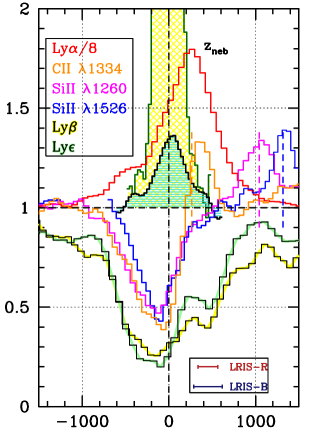
Figure 27.— (Left:) The relationship between the strength of interstellar resonance absorption lines (the average of Si II $\lambda 1260$ and $\lambda 1526$ (solid red points)) and that of the associated excited fine structure emission lines (Si II${}^{\ast}\lambda 1264$ and $\lambda 1533$; open magenta points) versus $\langle W_{\lambda}(\rm Ly\alpha)\rangle$ (see Figure 21.) There is a strong trend of non-resonance emission strength increasing relative to resonance absorption line strength as $\langle W_{\lambda}(\rm Ly\alpha)\rangle$ increases. The blue open squares in the bottom panel are the values of $1-f_{\rm c}$ determined using the “holes” model (§9.4.2), and are the same as those shown in the top panel of Figure 25. (Right:) As in Figure 21, for the subset of KLCS with nebular redshifts to show the non-resonant emission line kinematics with respect to $\rm Ly\alpha$ emission and the strong IS resonance absorption features. The green shaded emission feature is the average of the Si II${}^{\ast}\lambda 1265$ and Si II${}^{\ast}\lambda 1533$ profiles in the same composite; the equivalent width measurements for this particular composite are indicated with black open symbols in the lefthand panel. The yellow-shaded emission line is the mean [O III]$\lambda 5008$ emission line of the same subsample.

Figure 27 compares the mean equivalent widths of the resonance lines Si II$\lambda 1260$ and Si II$\lambda 1526$ with the average equivalent width of the non-resonant emission lines Si II${}^{\ast}\lambda 1265$ and Si II${}^{\ast}1533$ as a function of $W_{\lambda}(\rm Ly\alpha)$ for the KLCS sub-samples. The lefthand panel of Figure 27 shows the well-established anti-correlation between $W_{\lambda}(\rm Ly\alpha)$ and $W_{\lambda}$(LIS) (e.g., Shapley et al. 2003; Du et al. 2018) where LIS refers to low-ionization resonance absorption lines (red filled points). In addition, the ratio of Si II^∗ emission (skeletal points) to Si II absorption increases with $\langle W_{\lambda}(\rm Ly\alpha)\rangle$ – there is a weak trend of increasing strength of $W_{\lambda}$(Si II^∗ with $\langle W_{\lambda}(\rm Ly\alpha)\rangle$ (magenta dashed line in Figure 27) but a strongly decreasing trend of $W_{\lambda}$(Si II) with increasing $\langle W_{\lambda}(\rm Ly\alpha)\rangle$ causes the ratio $W_{\lambda}$(Si II${}^{\ast})/W_{\lambda}$(Si II) to vary from $\sim 0.3$ to $\sim 0.9$ across the sample.

Although a detailed discussion of the implications of the non-resonant emission is deferred to future work, one interpretation of the trends illustrated in Figure 27 is that the physical extent of the scattering medium producing resonance absorption lines in “down the barrel” spectra is more compact for galaxies with higher LyC escape fractions. In such a scenario, the KLCS spectroscopic aperture (projected physical size $9.2\times 10.3$ kpc at $\langle z_{\rm s}\rangle$) contains a significantly larger fraction of the gas with log $N_{\rm HI}\lower 2.15277pt\hbox{$\;\buildrel>\over{\sim}\;$}10^{17}$ cm^-2 in the CGM of galaxies having the highest LyC escape fraction. In other words – not surprisingly – galaxies are more likely to leak along an observed line of sight when they exhibit more spatially compact distributions of optically-thick gas in the interface between the ISM and CGM.

An interesting question is whether the more compact distribution of optically thick material is the “cause” or the “effect” of higher LyC escape. It is quite possible that the low-ionization CGM is reduced by a more intense local ionizing radiation field in the inner CGM. That is, the reduced spatial extent of optically-thick low-ionization material surrounding LyC leaking galaxies might be caused at least in part by self-ionization. For example, we consider the $W_{\lambda}(\rm Ly\alpha)$ (Q4) subsample, which has $\nu L_{\nu}(1500\textrm{\AA})\simeq 1.6\times 10^{11}L_{\odot}$ and $\mbox{$\langle f_{900}/f_{1500}\rangle_{\rm out}$}\simeq 0.17$ (Table 6), thus producing an average escaping ionizing luminosity $\langle\nu L_{\nu}(\textrm{LyC})\rangle\simeq 10^{44}$ ergs s^-1. The average specific intensity at the Lyman limit as a function of galactocentric distance $r$ would be $\langle I_{\nu}(r)\rangle\simeq 10^{-19}(r/50~{}{\rm kpc})^{-2}$ ergs s^-1 cm^-2 Hz^-1: at $r=50$ kpc, the local ionizing radiation field intensity would exceed that of the metagalactic background by a factor of $>10$, and could dominate the ionization state of the CGM to $r\lower 2.15277pt\hbox{$\;\buildrel>\over{\sim}\;$}150$ kpc around individual galaxies.

11.4. Ionizing Emissivity of $z\sim 3$ LBGs

Quantitative measurement of LyC flux from the KLCS sample of galaxies at $z\sim 3$ is the first step in addressing the issue of the connection between directly-observed galaxy properties and the propensity to leak significant LyC radiation. We have shown that even this step has required combining $N\sim 30$ independent galaxy spectra according to various easily-measured empirical criteria in order to accurately correct the ensemble for the effects of intergalactic and circumgalactic gas along our line of sight.

If the KLCS galaxy sample were a representative subset of the population of star-forming galaxies that contributes to the metagalactic ionizing radiation field at $z\sim 3$, then the values of $\langle f_{900}/f_{1500}\rangle_{\rm out}$ in Table 6 are all that is needed to convert a measurement of the far-UV (non-ionizing) emissivity $\epsilon_{\rm uv}=\int L_{\rm uv}\Phi(L_{\rm uv})dL_{\rm uv}$, where $\Phi(L_{\rm uv})$ is the galaxy luminosity function evaluated in the rest-frame FUV (typically 1500-1700 Å), into the ionizing emissivity contributed by the same population of galaxies,

$$\epsilon_{\rm LyC}\simeq\int_{L_{\rm uv,min}}^{L_{\rm uv,max}}\langle f_{900}/f_{1500}\rangle_{\rm out}\times L_{\rm uv}\Phi(L_{\rm uv})dL_{\rm uv}$$ (20)

as discussed by many authors (see, e.g., Steidel et al. 2001; Shapley et al. 2006; Nestor et al. 2011, 2013; Mostardi et al. 2013; Grazian et al. 2017.) This method is especially useful because $\Phi(L_{\rm uv})$ has been measured over a substantial range in $M_{\rm uv}$ at redshifts $z\simeq 2-9$ (e.g., Reddy & Steidel 2009; Oesch et al. 2010; Bouwens et al. 2015; Finkelstein et al. 2015; Parsa et al. 2016.)

Note that $\langle f_{900}/f_{1500}\rangle_{\rm out}$ appears inside the integral in equation 20; as discussed in the previous section, although KLCS samples only a limited range in $M_{\rm uv}$ ($-19.5\lower 2.15277pt\hbox{$\;\buildrel>\over{\sim}\;$}M_{\rm uv}\lower 2.15277pt\hbox{$\;\buildrel>\over{\sim}\;$}-22.1$; $0.25\lower 2.15277pt\hbox{$\;\buildrel<\over{\sim}\;$}L_{\rm uv}/L_{\rm uv}^{\ast}\lower 2.15277pt\hbox{$\;\buildrel<\over{\sim}\;$}3$), evidently only the UV-fainter half of the sample has significant $\langle f_{900}/f_{1500}\rangle_{\rm out}$. We argued in §11.1 that a surprisingly tight relationship between the covering fraction $f_{\rm c}$ and the measured $W_{\lambda}(\rm Ly\alpha)$ in the spectroscopic aperture suggests that the most direct signature of leaking LyC emission appears to be $W_{\lambda}(\rm Ly\alpha)$, and that the apparent dependence on $L_{\rm uv}$ is secondary. However, it is straightforward to obtain approximate numbers for the contribution of KLCS-like galaxies to $\epsilon_{\rm LyC}$ using the empirical dependence of $\langle f_{900}/f_{1500}\rangle_{\rm out}$ on either $L_{\rm uv}$ or $W_{\lambda}(\rm Ly\alpha)$.

11.4.1 Weighting by $L_{\rm uv}$

If we adopt the rest-frame FUV galaxy luminosity function (UVLF) determined by Reddy & Steidel (2009) for star-forming galaxies at $2.7\lower 2.15277pt\hbox{$\;\buildrel<\over{\sim}\;$}z\lower 2.15277pt\hbox{$\;\buildrel<\over{\sim}\;$}3.4$,

$$\Phi(L_{\rm uv})=\Phi^{\ast}\left(L_{\rm uv}/L_{\rm uv}^{\ast}\right)^{\alpha}{\rm exp}\left(-L_{\rm uv}/L_{\rm uv}^{\ast}\right),$$ (21)

with $\alpha=-1.73$, $\Phi^{\ast}=1.71\times 10^{-3}$ Mpc^-3, and $M_{\rm uv}^{\ast}=-21.0$, then the total FUV emissivity of the population of galaxies with $M_{1700}<-17.4$ (i.e., $L_{\rm uv}>0.036L_{\rm uv}^{\ast}$) is $\epsilon_{\rm uv}=3.28\pm 0.24\times 10^{26}$ ergs s^-1 Hz^-1 Mpc^-3. The KLCS dataset includes only galaxies with $M_{\rm uv}\leq-19.5$, sampling a range in $L_{\rm uv}$ that accounts for $\simeq 0.52\times\epsilon_{\rm uv}\simeq 1.71\times 10^{26}$ ergs s^-1 Hz^-1 Mpc^-3.

Note that the UV emissivity of the $M_{\rm uv}<-19.5$ population is relatively insensitive to the choice of UVLF: for example, if instead of Reddy & Steidel (2009) we were to use the parameters advocated by Parsa et al. (2016), i.e., $M_{\rm uv}^{\ast}\simeq-20.5$, $\alpha\simeq-1.37$, and $\epsilon_{\rm uv}\simeq 3.16\times 10^{26}$ ergs s^-1 Hz^-1 Mpc^-3 integrated down to $M_{\rm uv}\simeq-15.5$, then galaxies with $M_{\rm uv}<-19.5$ produce $\epsilon_{\rm uv}\simeq 0.48\times 3.16\times 10^{26}\simeq 1.52\times 10^{26}$ ergs s^-1 Hz^-1 Mpc^-3 at $\langle z_{\rm s}\rangle=3.05$, a difference of only $\simeq 11$%. Similarly, the fractional contribution of galaxies with $M_{\rm uv}<-19.5$ to the total emissivity integrated down to a common $M_{\rm uv}\simeq-15.5$ are 43% (Reddy & Steidel 2009) and 48% (Parsa et al. 2016.)

If we assume for the moment that $\langle f_{900}/f_{1500}\rangle_{\rm out}$$=0$ for galaxies with $M_{\rm uv}\leq-21.0$ and $\langle f_{900}/f_{1500}\rangle_{\rm out}$$=0.11$ for $-21<M_{\rm uv}\leq 19.5$ (Table 6 and Figure 17), then the galaxies that contribute significantly to $\epsilon_{\rm LyC}$ at $z\sim 3$ have $\epsilon_{\rm uv}\simeq 1.21\times 10^{26}$ ergs s^-1 Hz^-1 Mpc^-3 and thus contribute $\epsilon_{\rm LyC}\simeq 0.11\times 1.21\times 10^{26}\simeq 13.0\times 10^{24}$ ergs s^-1 Hz^-1 Mpc^-3. The contribution would be slightly lower, $\epsilon_{\rm LyC}\simeq 11\times 10^{24}$ ergs s^-1 Hz^-1 Mpc^-3, assuming $\langle f_{900}/f_{1500}\rangle_{\rm out}$$=0.094$ as for the “IGM Only” transmission model.

11.4.2 Weighting by $W_{\lambda}(\rm Ly\alpha)$

Alternatively, we can use our derived empirical relation between $W_{\lambda}(\rm Ly\alpha)$ and $\langle f_{900}/f_{1500}\rangle_{\rm out}$ to estimate the contribution of KLCS-like galaxies to $\epsilon_{\rm LyC}$. In this case, we take $\langle f_{900}/f_{1500}\rangle_{\rm out}$ outside the integral in equation 20 and use the distribution function $n[W_{\lambda}(\rm Ly\alpha)]$ of UV continuum-selected $z\sim 3$ galaxies to estimate contributions to $\epsilon_{\rm LyC}$ relative to the integral over the UVLF, $\epsilon_{\rm uv}$.

We begin with equation 19, the best linear relation between $\langle f_{900}/f_{1500}\rangle_{\rm out}$ and $W_{\lambda}(\rm Ly\alpha)$; where again the statistic $\langle f_{900}/f_{1500}\rangle_{\rm out}$ is adopted as the least model-dependent link between the FUV luminosity of galaxies and their contribution to the ionizing emissivity, since it does not depend on assumptions regarding SPS models, ISM radiative transfer, or attenuation by dust. However, for the present purpose, we assume that $W_{\lambda}(\rm Ly\alpha,{\rm CaseB})\simeq 110$ Å as discussed in §11.1 above, and a model for mapping between $\langle f_{900}/f_{1500}\rangle_{\rm out}$ and $W_{\lambda}(\rm Ly\alpha)$ given by equation 19. For $W_{\lambda}(\rm Ly\alpha)>0.5W_{\lambda}(\rm Ly\alpha,{\rm CaseB})=55$ Å, which is unconstrained by the KLCS composite spectra, we assume that $\langle f_{900}/f_{1500}\rangle_{\rm out}$ reaches a maximum when $(W_{\lambda}(\rm Ly\alpha)/110~{}\textrm{\AA})\sim 0.5$, since at some point the increasing escape of LyC photons would result in a decreasing $\rm Ly\alpha$ source function compared to Case B expectations. A naive expectation is that the source function of $\rm Ly\alpha$ emission along a particular line of sight would be reduced by a factor (1-$f_{\rm c}$) relative to Case B, followed by a further reduction proportional to $f_{\rm c}$ due to scattering of $\rm Ly\alpha$ photons by the covered portion of the UV continuum. In such a simplified picture, one might expect $W^{\prime}\equiv W_{\lambda}(\rm Ly\alpha)/W_{\lambda}(\rm Ly\alpha,{\rm CaseB})\approx 2f_{\rm c}(1-f_{\rm c})$, which has a maximum $W^{\prime}\approx 0.5$ when $f_{\rm c}\simeq 0.5$ and goes to zero as $f_{\rm c}\rightarrow 0$ and as $f_{\rm c}\rightarrow 1$. Solving for $f_{\rm c}$ in terms of $W^{\prime}$ gives

$$(1-f_{\rm c})=0.5-\left[|0.5W^{\prime}-0.25|\right]^{1/2}.$$ (22)

Using equation 19 and the holes model fit $(1-f_{\rm c})\approx 0.75W^{\prime}$ (Figure 25) to connect $\langle f_{900}/f_{1500}\rangle_{\rm out}$ to $1-f_{\rm c}$ over the range constrained by the data results in a model which maps the expected $\langle f_{900}/f_{1500}\rangle_{\rm out}$ to $W^{\prime}$ over the full range of each:

$$\mbox{$\langle f_{900}/f_{1500}\rangle_{\rm out}$}\simeq 0.28-\left[|0.146W^{\prime}-0.073|\right]^{1/2}.$$ (23)

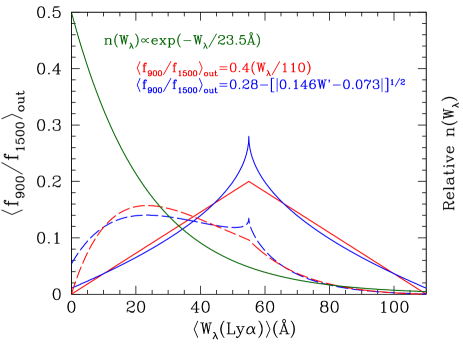
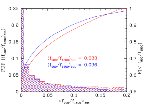
Figure 28.— (Top:) Estimated $\langle f_{900}/f_{1500}\rangle_{\rm out}$ as a function of $W_{\lambda}(\rm Ly\alpha)$. The red and blue solid curves correspond to the distribution functions of the same color coding in the legend. The dark green curve shows the relative incidence of $W_{\lambda}(\rm Ly\alpha)$ for a continuum-selected spectroscopic sample, which weights the incidence of the values of $\langle f_{900}/f_{1500}\rangle_{\rm out}$ expected in an ensemble. The dashed curves show the expected distribution of $W_{\lambda}(\rm Ly\alpha)$ weighted by the relative contribution to the total LyC emissivity, i.e., proportional to $n[W_{\lambda}]\times\mbox{$\langle f_{900}/f_{1500}\rangle_{\rm out}$}$. (Bottom:) The probability distribution function for $\langle f_{900}/f_{1500}\rangle_{\rm out}$ for an ensemble of LBGs, accounting for the distribution functions in the top panel for $\langle W_{\lambda}(\rm Ly\alpha)\rangle>0$ and assuming that 40% of the ensemble has spectroscopic $\langle W_{\lambda}(\rm Ly\alpha)\rangle<0$ (i.e., $\rm Ly\alpha$ in net absorption.) The solid curves refer to the righthand axis, showing the cumulative fraction with lower $\langle f_{900}/f_{1500}\rangle_{\rm out}$. The ensemble averages for the two distributions are indicated with the same color coding.

Two models mapping $\langle f_{900}/f_{1500}\rangle_{\rm out}$ to $W_{\lambda}(\rm Ly\alpha)$ are illustrated in the top panel of Figure 28; one is the best linear relation from equation 19, reflected about $W^{\prime}=0.5$, the assumed maximum. The second is based on equation 23. Also shown in the top panel of Figure 28 is the relative incidence of $W_{\lambda}(\rm Ly\alpha)$ parametrized as an exponential of the form $n(W_{\lambda})\propto{\rm exp}(-W_{\lambda}/W_{0})$, with $W_{0}=23.5$ Å, very close to the observed distribution function in the KLCS sample, as well as that obtained from previous spectroscopic samples at $z\sim 3$ (Shapley et al. 2003; Kornei et al. 2010.) Reddy et al. (2008) showed that the observed distribution of $W_{\lambda}(\rm Ly\alpha)$ at $z\sim 3$ must be close to the intrinsic distribution for the galaxies contributing to the FUV continuum luminosity function. We further assume that $\simeq 40$% of continuum-selected galaxies have spectroscopic $W_{\lambda}(\rm Ly\alpha)\leq 0$ (and therefore have $\langle f_{900}/f_{1500}\rangle_{\rm out}$$\simeq 0$). It is then straightforward to compute the probability distribution of $\langle f_{900}/f_{1500}\rangle_{\rm out}$ expected for an ensemble of continuum-selected galaxies with $M_{\rm uv}<-19.5$ ($L_{\rm uv}>0.25L_{\rm uv}^{\ast}$) as in the KLCS sample. The resulting PDFs of the quantity $\langle f_{900}/f_{1500}\rangle_{\rm out}$ for an ensemble of galaxies with the assumed $n[W_{\lambda}(\rm Ly\alpha)]$ are shown in the bottom panel of Figure 28. Note that just over 50% of the PDF falls in lowest bin of $\langle f_{900}/f_{1500}\rangle_{\rm out}$  but the ensemble average is $\langle f_{900}/f_{1500}\rangle_{\rm out}$$\simeq 0.035$.

Returning to the estimate of the contribution to $\epsilon_{\rm LyC}$, the $W_{\lambda}(\rm Ly\alpha)$-based $\mbox{$\langle f_{900}/f_{1500}\rangle_{\rm out}$}=0.035$ implies that galaxies with $M_{\rm uv}<-19.5$ contribute $\epsilon_{\rm LyC}\simeq 0.035\times\times 1.71\times 10^{26}\simeq 5.9\times 10^{24}$ ergs s^-1 Hz^-1 Mpc^-3. Because of the strong empirical connection between $\langle f_{900}/f_{1500}\rangle_{\rm out}$ and $W_{\lambda}(\rm Ly\alpha)$, and because previous work has shown that spectroscopic samples are unbiased with respect to $W_{\lambda}(\rm Ly\alpha)$, we are more confident of the $W_{\lambda}(\rm Ly\alpha)$-based estimate of $\epsilon_{\rm LyC}$ than of the luminosity-weighted estimate in §11.4.1.

For comparison, recent indirect estimates of the total ionizing emissivity at $z\sim 3$ inferred from modeling the transfer of ionizing radiation through the IGM coupled with measurements of the mean transmissivity of the Lyman $\alpha$ forest (Becker & Bolton 2013) find $\epsilon_{\rm LyC}\simeq 10\times 10^{24}$ ergs s^-1 Hz^-1 Mpc^-3 with a systematic uncertainty of $\sim 0.4$ dex (factor of 2.5). . Thus, without extrapolating our results to lower luminosities that are not directly constrained by the KLCS sample, the ionizing emissivity $\epsilon_{\rm LyC}[L_{\rm uv}>0.25L_{\rm uv}^{\ast}]\simeq 5.9\times 10^{24}$ ergs s^-1 Hz^-1 Mpc^-3 comprises $\sim 60$% of the estimated total. In addition, it exceeds the total ionizing emissivity of QSOs at $z\sim 3$, estimated to lie in the range $\simeq 1.6-5\times 10^{24}$ ergs s^-1 Hz^-1 Mpc^-3 (Hopkins et al. 2007; Cowie et al. 2009.)

A more detailed discussion of the implications of our result for the ionizing emissivity $\epsilon_{\rm LyC}$ and photoionization rate $\Gamma$ at $z\sim 3$, as well as a comprehensive comparison to other observational constraints, is deferred to a separate paper.

12. Summary and Discussion

We have presented the results of a deep spectroscopic survey of $\langle z\rangle=3.05\pm 0.18$ Lyman-break-selected sources obtained using LRIS-B+R on the Keck 1 telescope. The spectra cover the observed wavelength range $3200-7200$ Å  with spectral resolving power of $R=800-1400$, enabling direct measurement of the rest-frame LyC region $880\leq\lambda_{0}/\textrm{\AA}\leq 910$ for sources with redshifts $z>2.75$, as well as the far-UV spectrum over the range $930\lower 2.15277pt\hbox{$\;\buildrel<\over{\sim}\;$}\lambda_{0}/\textrm{\AA}\lower 2.15277pt\hbox{$\;\buildrel<\over{\sim}\;$}1800$. Very careful attention was paid to minimizing systematic errors associated with flat-fielding, background subtraction, and spectral extraction. In addition, the initial sample of 136 spectra was carefully examined to remove those contaminated by foreground (lower-redshift) galaxies or affected by other potential systematic errors. The final KLCS sample of 124 galaxies spans a UV luminosity range $-19.5\lower 2.15277pt\hbox{$\;\buildrel>\over{\sim}\;$}M_{\rm uv}\lower 2.15277pt\hbox{$\;\buildrel>\over{\sim}\;$}-22.0$ ($0.25\lower 2.15277pt\hbox{$\;\buildrel<\over{\sim}\;$}(L_{\rm uv}/L^{\ast}_{\rm uv})\lower 2.15277pt\hbox{$\;\buildrel<\over{\sim}\;$}3$), and is representative of the larger spectroscopic parent samples from which it was drawn.

Of the 124 individual galaxies in the final KLCS sample, 15 (12%) have formal spectroscopic detections ($f_{900}\geq 3\sigma_{900}$) of residual LyC flux; the remainder have typical 2$\sigma$ upper limits $f_{900}\lower 2.15277pt\hbox{$\;\buildrel<\over{\sim}\;$}0.014~{}\mu$Jy ($m_{\rm AB}\lower 2.15277pt\hbox{$\;\buildrel>\over{\sim}\;$}28.5$) averaged over the narrow rest-frame bandpass $880\leq\lambda_{0}\leq 910$ Å.

Measurements of the emergent LyC emissivity of galaxies are limited both by the dynamic range of individual spectra and – more importantly – by large and stochastic variations in IGM transmission for individual lines of sight averaged over the LyC measurement band [880,910] Å. Because of the importance of an accurate statistical model of the opacity of gas lying outside of the galaxy ISM, but between the source and the observer, to measurement of the emergent ratio of ionizing to non-ionizing flux density ratio $\langle f_{900}/f_{1500}\rangle_{\rm out}$, we used the statistics of H I measured in both the general IGM and in the CGM of galaxies from the Keck Baryonic Structure Survey (KBSS; Rudie et al. 2013) to produce new Monte Carlo simulations of the IGM transmission as a function of source redshift. These simulations were used to model the transmission for individual sightlines at a given source redshift, and to predict the average transmission for ensembles of sources with the same redshift distribution as the real KLCS sample.

We focused our analysis on composite spectra formed from subsets sharing common attributes that are easily measured from individual spectra. The ensemble spectra have much higher S/N than individual measurements, thus substantially increasing the dynamic range for LyC detection; in addition, the sub-sample sizes have been chosen so that the marginalized IGM+CGM transmission expected for the ensemble is known accurately. The mean transmission appropriate to each ensemble was used to correct the observed flux density ratio $\langle f_{900}/f_{1500}\rangle_{\rm obs}$ to the more relevant emergent flux density ratio $\langle f_{900}/f_{1500}\rangle_{\rm out}$ without adding significant additional uncertainty.

Our main results may be summarized as follows:

$\bullet$ Averaged over the full KLCS sample, we find $\langle f_{900}/f_{1500}\rangle_{\rm out}=0.057\pm 0.006$. This value is independent of the nature of the ionizing sources within the galaxies, and is model-independent except for small residual uncertainties in the IGM+CGM transmission; the same value, within statistical uncertainties, is found for galaxies in the lowest and highest quartile in redshift. However, we find two other galaxy characteristics that correlate strongly with the propensity to leak measurable LyC radiation: rest-frame UV luminosity ($L_{\rm uv}$) and rest-frame Lyman-$\alpha$ equivalent width [$W_{\lambda}(\rm Ly\alpha)$]. In particular, galaxies belonging to the lowest quartile ($\langle L_{\rm uv}/L^{\ast}_{\rm uv}\rangle\simeq 0.5$) have $\langle f_{900}/f_{1500}\rangle_{\rm out}=0.138\pm 0.024$, while the highest quartile ($\langle L_{\rm uv}/L^{\ast}_{\rm uv}\rangle\simeq 1.7$) have $\langle f_{900}/f_{1500}\rangle_{\rm out}=0.000\pm 0.003$). Similarly, galaxies in the highest quartile of $\rm Ly\alpha$ equivalent width ($\langle W_{\lambda}(\rm Ly\alpha)\rangle=42$ Å) have $\langle f_{900}/f_{1500}\rangle_{\rm out}=0.166\pm 0.025$, while the lowest quartile ($\langle W_{\lambda}(\rm Ly\alpha)\rangle=-18$ Å) have $\langle f_{900}/f_{1500}\rangle_{\rm out}=0.013\pm 0.011$.

$\bullet$ We show that trends in LyC emission are strongly linked to the apparent depth, relative to the continuum, of low-ionization metal lines and, especially, the depth of Lyman series absorption lines (other than $\rm Ly\alpha$), which always indicate a higher covering fraction than the metal lines (§9.3.) In most cases, there is evidence for strong saturation among these ISM absorption features, suggesting that the apparent depth of the features is directly related to the continuum covering fraction of neutral gas with appreciable $N_{\rm HI}$. The $\rm Ly\alpha$ emission line equivalent width $W_{\lambda}(\rm Ly\alpha)$, long known to be inversely correlated (and probably causally connected) to the low-ion absorption line strength (e.g., Shapley et al. 2003; Steidel et al. 2010, 2011) is a manifestation of the effect of the same gas on the emergent EUV/FUV spectrum.

$\bullet$ We use the results above to explore more model-dependent characterizations of the LyC emission from the galaxies, including the relative and absolute escape fraction of ionizing photons from the parent galaxies, $f_{\rm esc,rel}$, $f_{\rm esc,abs}$ respectively. We show (§9.2) that the non-ionizing (i.e., 920-1750 Å) composite FUV spectra can be very well matched by SPS models with low stellar abundance ([Fe/H]$\sim-1.15$; $Z_{\ast}/Z_{\odot}\simeq 0.07$) which include binary evolution of massive stars reddened by plausible far-UV attenuation relations. These models have intrinsic $L_{900}/L_{1500}\simeq 0.28\pm 0.03$ over the plausible range of star formation age $7.5\lower 2.15277pt\hbox{$\;\buildrel<\over{\sim}\;$}{\rm log(t/yr)}\lower 2.15277pt\hbox{$\;\buildrel<\over{\sim}\;$}8.7$, corresponding to $\xi_{\rm ion}\simeq 25.5\pm 0.1$.

$\bullet$ We show (§9.4.1 and §9.4.2) that the same SPS and attenuation models can be used with simple geometrical models of the ISM to simultaneously account for the depth of the Lyman series absorption lines, the residual LyC emission, the damping wings of the $\rm Ly\alpha$ absorption profile (which constrains $N_{\rm HI}$ in the dominant absorbing gas) as well as the stellar FUV spectrum. The best-fit models provide constraints on $N_{\rm HI}$, the continuum covering fraction $f_{\rm c}$, and the intrinsic and escaping fraction of both ionizing and non-ionizing stellar photons.

$\bullet$ We examine in more detail (§11.1) the tight relationship between $W_{\lambda}(\rm Ly\alpha)$ and the inferred uncovered portion $(1-f_{\rm c})$ measured from model fits to the composite spectra. For our favored model geometry, in which both LyC and a fraction of $\rm Ly\alpha$ photons escape along the line of sight through the same “holes” in the ISM, the average LyC escape fraction for KLCS galaxies at $z\sim 3$ is $\langle f_{\rm esc,abs}\rangle=0.09\pm 0.01$. Within the sample, $\langle f_{\rm esc,abs}\rangle\simeq\langle 1-f_{\rm c}\rangle$ varies linearly with the observed $\langle W_{\lambda}(\rm Ly\alpha)\rangle$ (§11.1), over the range $0\lower 2.15277pt\hbox{$\;\buildrel<\over{\sim}\;$}\langle f_{\rm esc,abs}\rangle\lower 2.15277pt\hbox{$\;\buildrel<\over{\sim}\;$}0.29$ and $0\leq W_{\lambda}(\rm Ly\alpha)/{\textrm{\AA}}\lower 2.15277pt\hbox{$\;\buildrel<\over{\sim}\;$}50$. We argue that the kinematics of $\rm Ly\alpha$ emission are not uniquely connected with the propensity to leak LyC radiation into the IGM; rather, it is the presence of holes (parametrized by $\langle 1-f_{\rm c}\rangle$) in the scattering/absorbing medium along our line of sight which apparently controls both $W_{\lambda}(\rm Ly\alpha)$ and $\langle f_{900}/f_{1500}\rangle_{\rm out}$.

$\bullet$ Finally, we use the observed interrelation of $L_{\rm uv}$, $f_{\rm c}$, $W_{\lambda}(\rm Ly\alpha)$, and $\langle f_{900}/f_{1500}\rangle_{\rm out}$ to estimate the contribution of galaxies with $M_{\rm uv}<-19.5$ to the total ionizing emissivity $\epsilon_{\rm LyC}$ at $z\sim 3$ (§11.4). Because the correlation between the spectroscopically-measured $W_{\lambda}(\rm Ly\alpha)$ and inferred $\langle f_{\rm esc,abs}\rangle$ is both strong and linear, our most confident estimate comes from integrating the non-ionizing UVLF weighted by the product $n[W_{\lambda}(\rm Ly\alpha)]\times\mbox{$\langle f_{900}/f_{1500}\rangle_{\rm out}$}$, where $n[W_{\lambda}(\rm Ly\alpha)]$ is the relative incidence of $W_{\lambda}(\rm Ly\alpha)$ and $\langle f_{900}/f_{1500}\rangle_{\rm out}$ is the empirically-measured ionizing to non-ionizing continuum ratio evaluated as a function of $W_{\lambda}(\rm Ly\alpha)$. We find a mean effective $\langle f_{900}/f_{1500}\rangle_{\rm out}$$\sim 0.035$ for galaxies with $-19.5\geq M_{\rm uv}\geq-22.1$, accounting for $\lower 2.15277pt\hbox{$\;\buildrel>\over{\sim}\;$}50$% of the total $\epsilon_{\rm LyC}$ estimated using indirect methods, and exceeding by a factor of $\sim 1.2-3.7$ the total ionizing emissivity of QSOs at $z\sim 3$.

Throughout this paper, we have deliberately concentrated on the least model-dependent, most easily-measurable parameters – UV luminosity and $W_{\lambda}(\rm Ly\alpha)$ – in seeking significant trends between galaxy properties and the propensity to leak significant LyC flux. There has recently been a great deal of interest in identifying observational signatures that strongly correlate with LyC escape but are more amenable to measurement at very high redshift where direct measurements of LyC flux become difficult (e.g., Steidel et al. 2011; Heckman et al. 2011; Zackrisson et al. 2013; Nakajima & Ouchi 2014; Erb et al. 2014; Trainor et al. 2015, 2016; Verhamme et al. 2017). Among the most promising indirect indicators discussed are anomalous nebular line ratios, possibly due to density-bounded H II regions, where nebular emission from lower-ionization species (such as [OII] or [SII]) may be suppressed. One proposed manifestation is a large value of the ratio ${\rm O32\equiv I([OIII]4960+5008)/I([OII]3727+3729)}$, which has the advantage of being easily-observable by JWST in the redshift range $z\simeq 6-9$. The subset of the KLCS sample with $z>2.92$, comprising 94 of 124 galaxies in the sample (76%), allows measurement of [O III] $\lambda\lambda 4960$, 5008 and [O II] $\lambda\lambda 3727$,3729 in the K and H atmospheric windows from the ground. We are currently completing Keck/MOSFIRE observations of the relevant KLCS sub-sample to investigate correlations between these excitation/ionization-sensitive line ratios and direct LyC observations. The results will be presented in future work.

Deep ground-based near-IR photometry, Spitzer/IRAC coverage, and selected coverage with deep HST WFC3-IR and ACS imaging are also well underway - these observations, when completed, will provide stellar population parameters for all of KLCS. The HST observations will serve as a final verification that the sample has been cleaned of all contaminating sources. Additionally, in view of the apparently-strong anti-correlation with UV luminosity and UV reddening (§8; Reddy et al. 2016b) and positive correlation with $W_{\lambda}(\rm Ly\alpha)$ of the LyC escape fraction, we are in the process of extending KLCS to fainter UV luminosities, bluer UV colors, and stronger $W_{\lambda}(\rm Ly\alpha)$ using Keck/LRIS-B+R.

Continued development of state-of-the-art stellar population synthesis models (e.g., Eldridge et al. 2017; Choi et al. 2017), particularly those focusing on the rest-frame UV, will clearly be important to modeling the sources of LyC emission in a fully-consistent treatment including the stars, gas, and dust in forming galaxies. “Rules of thumb” established at $z\simeq 3$ will be crucial to interpreting sources at much higher redshift where only indirect measurements are possible.

Appendix A KLCS Data Reduction Details

A.1. Scattered Light and Flat-Fielding

As discussed in §4, adequate illumination for spectroscopic flat-fields necessitates the use of twilight sky, observations. However, because of the rapidly increasing system sensitivity as wavelength increases from 3100 Å to 4000 Å, it is difficult in practice (particularly given the very short periods of evening and morning twilight on Mauna Kea) to obtain good exposures in the deep UV while controlling the amount of stray light reaching the LRIS-B detector.

Extensive tests performed during several LRIS observing runs established that stray light at a very low level was adversely affecting the LRIS-B observations, particularly at the shortest wavelengths where the sky background is faintest. We found that most of the problem could be attributed to stray light present in the twilight sky flat fields, which were invariably obtained just after sunset (or just before sunrise). Evidently scattering of sky light inside the telescope dome allowed low-level, undispersed stray light to reach the LRIS-B detector, which would then imprint diffuse undulations in the background level in flat-fielded science exposures. These subtle fluctuations had a significant effect on the precision of subsequent background subtraction.

Once the problem was identified, we adopted an improved strategy for obtaining twilight sky flat-fields: for each slitmask we obtained two sets of exposures, one of which had the LRIS-B $U_{\rm n}=u^{\prime}$ filter (bandpass 3500/600 Å) inserted in the beam. The $U_{n}$ filter cuts off longward of $\sim 3900$ Å and efficiently blocks the vast majority of stray light, since the LRIS-B filters are inserted just in front of the spectrograph camera. The presence of the filter made it possible to safely obtain flat field exposures with higher signal-to-noise ratio (S/N) shortward of $3900$ Å. The $U_{\rm n}$ twilight spectroscopic images were then combined with shorter twilight sky exposures taken without the filter in place. Since most of the stray light problem was confined to regions with $\lambda<3900$ Å, the two sets of flats were “spliced” together to create composite twilight sky flats with high S/N throughout the $3200$ Å$-5000$ Å wavelength range, with greatly reduced contamination by scattered light.

A.2. Image Rectification

After bias subtraction and CCD gain correction, the relevant “footprint” on the spectroscopic frames are identified by tracing the slit edges across the dispersion direction, fitting the edge positions with a 3rd order polynomial that is then used to extract each slit and transform it into a rectilinear image by applying nearest-integer pixel shifts in the spatial direction only. This produces a rectified slit image that requires no re-sampling of pixel intensities.

In the absence of differential atmospheric refraction, the previous step would make object traces run parallel to the CCD columns and thus simple linear traces could be used to extract one-dimensional (1D) spectra. For the data obtained prior to the ADC installation in July 2007, the wavelength dependence of objects within slits was accounted for, as described in §A.4.

A.3. Slit Illumination Correction

Imperfect milling or cleaning of LRIS slitmasks prior to insertion in the instrument can cause spatially-abrupt changes in slit illumination along the spatial direction, since (if everything is set up correctly) the slit plane is where both the telescope and the spectrograph camera are focused. This slit illumination function will also incorporate any intrinsic illumination gradients due to field-position-dependent vignetting within the telescope or instrument optics. Since our observations are attempting to detect signal at the level of $\lower 2.15277pt\hbox{$\;\buildrel<\over{\sim}\;$}1\%$ of the night sky background, the typical 1-2% divots in the slit function need to be corrected before the sky subtraction stage. Left uncorrected, small systematic deviation from zero mean might remain in the background subtracted images; in short exposures this problem can easily go unnoticed, as other sources of random error are dominant. However, its systematic influence becomes clear in the average of many exposures.

Custom procedures were developed to correct for variations in slit function for both science and calibration exposures, accounting for small amounts of instrument flexure between each and the images used for illumination correction (i.e., shifts in the positions of the slit edges, and therefore of any slit defects, on the detector.) The slit function for each slit on a mask was obtained from rectified two-dimensional spectrograms (§A.2) of the twilight sky by collapsing in the dispersion direction over the wavelength range deemed unaffected by residual scattered light, and averaging with iterative $\sigma$-rejection. The slit illumination correction was then applied to all rectified science and calibration exposures.

A.4. Atmospheric Dispersion Correction and
Object Tracing

Since we are interested both in detecting LyC flux when present, and obtaining sensitive upper limits when it is not, it is advantageous to be confident about the location of an object’s trace whether or not flux is evident. An often-used technique for tracing object positions in 2-D spectrograms is to determine spatial centroids regularly along the whole dispersion axis, which of course relies on the presence of signal over the same range. There is a tendency for traces extrapolated beyond the point where there is detectable flux to “wander” in search of upward fluctuations in the noise level. This is clearly undesirable in our particular application.

Prior to the deployment of the ADC on Keck 1, the trace of an object spectrum would differ from the trace of its slit edge by an amount determined by differential atmospheric refraction (DAR). Slitmask alignment for KLCS was always performed using direct imaging mode through the mask with a G-band filter in the LRIS-B beam, and guiding was maintained using an offset guide field CCD camera with peak sensitivity in V band. The exact value of the apparent spatial shift with time of source positions within slits depends on wavelength, airmass, slit position angle with respect to the elevation direction (the parallactic angle) and atmospheric conditions (temperature, pressure, water vapor pressure) at the time of observation. For reasons of practicality, KLCS observations were obtained (both before and after installation of the ADC) using a single mask and sky PA over a range of hour angle, albeit as close to the meridian as possible.

As a consequence, individual exposures of the same source could not be spatially registered at all wavelengths simultaneously. The difference in the apparent spatial position of the object over the 3200-5000 Å range of LRIS-B can be as large as $\sim 1$″($\sim 7-8$ LRIS-B pixels) if the slits have been oriented near the parallactic angle to minimize light losses due to DAR.

We developed an approach that deals with this problem in the earliest KLCS masks taken prior to August 2007. Using the atmospheric dispersion model of Filippenko (1982) we predict the value of the apparent spatial offset of the object position as a function of wavelength, and implement the shifts during the slit rectification step so that the object position in the rectified image is parallel to the slit edges, at a constant pixel location. Tests performed on observations of bright sources demonstrated that using the average atmospheric conditions for a given night on Mauna Kea provided sufficient precision in predicting the wavelength-dependent image shift from atmospheric dispersion. After August 2007, this procedure became unnecessary, as the ADC removes all but $\lower 2.15277pt\hbox{$\;\buildrel<\over{\sim}\;$}0.1$${}^{\prime\prime}~{}$ of differential shift over the full LRIS-B wavelength range.

A.5. Background Subtraction

Once careful slit illumination and flat-field corrections have been applied (§A.3 and §A.1), a low-order polynomial becomes an adequate description of the background intensity along the spatial direction. The accuracy of the background estimation depends to a large extent on the number of spatial pixels at each dispersion point that sample only “background” and not the outer parts of either the principal target or any part of nearby objects that happen to fall on the slit. Our experience has been that, at the level of sensitivity reached in the KLCS ($m_{AB}\sim 28.0$, or $\sim 2\times 10^{-31}$ ergs s^-1 cm^-2 Hz^-1,) the fraction of “clean” pixels remaining after source masking can be in the minority. We found it helpful, in terms of the number of spectra ultimately useful for LyC measurements, to enforce relatively long individual slits centered on high priority targets (slit lengths $>15$ arcsec), sometimes at the expense of the number of targets that could be accommodated on a single slitmask.

We also deliberately lowered the priority for slit assignment of objects lying in obviously crowded regions on the deep images. In spite of this pre-screening of potential targets, the majority of the slits included serendipitous sources detected in the vicinity of the primary target. In fact, after combining $\geq 8$ hours of LRIS spectroscopic observations the sensitivity is high enough to clearly detect the spectra of all sources seen in our deepest ground-based broad-band $G$ or ${\cal R}$ images, which typically reach $1\sigma$ limits of $G\sim 29.5$ and ${\cal R}\sim 28.8$ mag arcsec^-2; (Steidel et al. 2003, 2004). Using faint object positions predicted from the deep images we were in a position to exclude most or all pixels along the slit that might be contributing something other than sky background.

Background subtraction was performed in two stages: on the first pass we used object masks created from objects with significant detections in single 1800s LRIS-B exposures; in the second stage we compared the stack of the 2D background-subtracted spectrograms with broad band images and masked additional slit regions containing any source visible in either. An iterative fit with a polynomial function of order 2 to 4 was used to determine the final background model, which was subtracted separately for each 1800s exposure. The sky-subtracted spectrograms were then combined in 2-D, after shifting into spatial and spectral registration, by averaging, with bad pixel and outlier rejection.

The effectiveness of the above background subtraction procedures is discussed in more detail in §A.6.

A.5.1 Noise Model

Throughout the reduction process, care was taken to preserve the original pixel sampling and number of photoelectrons per pixel in order to track formal uncertainties through all steps. A stack of all science frames made just prior to the 2-D background subtraction stage was made as a record of the number of sky+object photoelectrons recorded in every pixel. These images are used to estimate the variance each pixel $[i,j]$ in the 2d spectrogram,

$$\sigma_{\rm pix}^{2}[i,j]=N_{\rm exp}[i,j]\times(C[i,j]+\rho^{2})~{},$$ (A1)

where $N_{\rm exp}$ is the number of 1800s exposures averaged to produce the value of pixel $[i,j]$, $C[i,j]$ is the number of photoelectrons recorded in the pixel, and $\rho$ is the detector read noise, assumed to be $\rho=3.8$e${}^{-}{\rm pix}^{-1}$ for LRIS-B.

A.6. Testing for Systematic Errors in 2D Spectrograms

In this section, we outline tests performed to assess the quality of data reduced as in §4.2. Most importantly, we tested for the presence of residual systematic errors in the 2-D background subtraction by creating an average two-dimensional spectrum for an ensemble of final 2-D background-subtracted spectrograms for a set of KLCS targets which each led to $>3\sigma$ detections of residual flux in the rest-frame [880-910] Å. Fully processed, background-subtracted two-dimensional rectified spectrograms were wavelength calibrated and then put onto a common observed wavelength grid; We used the same object masks that had been created in the second pass of the sky subtraction phase for each slit (§A.5), so that when the spectrograms were averaged, the masked pixels in each were excluded. The effective exposure time for the resulting stack [Figure 29] is $\sim 90$ hours, so that the random noise (due to photon statistics and detector read noise) is expected to be lower by a factor of $\simeq 3$ compared to any single observation in KLCS, thus more sensitive to possible systematic errors.

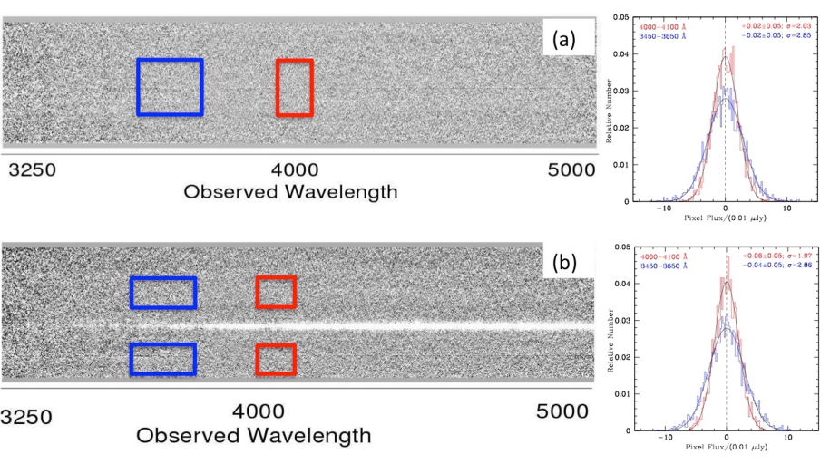
Figure 29.— (a) Two-dimensional composite spectrogram, combined using the object masks created during the background subtraction second pass, described in §A.5, for the 10 slits containing nominally detected LyC sources. Histograms of pixel fluxes, in units of 0.01 $\mu$Jy ($10^{-31}$ ergs s^-1 cm^-2 Hz^-1), are shown to the right for the regions indicated with colored boxes on the image: blue corresponds to the observed wavelength range 3450-3650 Å and red to the range $4000-4100$ Å, and both windows are 80 spatial pixels ($\simeq 10.8$ arcsec) wide. The values of the mean and standard error in the mean are shown for each histogram, along with the fitted value of $\sigma$ assuming zero mean and a normal distribution, as expected for regions on the 2-D images without background subtraction systematics and with no residual flux from unmasked objects. (b) Similar to (a), except that in this case, the primary target galaxy was left unmasked, and the 2-D spectrograms were registered spatially to place the target at a constant Y-pixel location. The pixel statistics within the colored boxes (shown at right) should be sensitive to possible systematic sky subtraction errors related to the position of the primary target along the slit. As the histograms show [based on the same total number of pixels in each sample as in (a)], the residuals are consistent with Gaussian noise with zero mean, and $\sigma_{\rm pix}$ values in the crucial 3450-3650 Å range are identical to within 0.3% to those in the same wavelength interval in (a).

The rms noise values within the boxes shown in Figure 29 are higher in the $3450-3650$ Å range due to lower system sensitivity (since the pixel intensity values are calibrated onto a flux density scale.) If the background subtraction is accurate, with systematics that are small compared to random errors, the distribution of pixel values is expected to well-described by a normal distribution with zero mean. The histograms to the right of the image show that this is the case for both wavelength regions. In addition, the measured rms noise level $\sigma$ is entirely consistent with the noise model described in §A.5.1 (see below).

As a second test for background subtraction systematics, we re-made the stacked composite spectrum using the same slits, but without masking the primary target galaxy (all other object masks remain the same). In this case, the spectrograms were spatially shifted before averaging so as to align the slit position of the primary target in the final image. The resulting two-dimensional stacked composite is presented in Figure 29(b); in this case, the stack would be sensitive to possible systematic errors that might be correlated with the position of the target object (generally the brightest object on the slit.) Unlike the previous case, which tested our ability to mask all significant sources in performing 2-D background subtraction, systematic errors in sky subtraction should become more prominent as more high-sensitivity spectrograms are averaged. To the right of Figure 29 are histograms of intensities drawn from regions on either side of the main target, beginning $\pm$4${}^{\prime\prime}\mskip-7.6mu.\,$0 from the target centroid, evaluated in the same rest-wavelength intervals as in Figure 29(a) (with the same total number of pixels, divided into two separate spatial regions). The results are very similar – with zero mean and essentially identical $\sigma$ within each wavelength region – to those obtained in Figure 29(a).

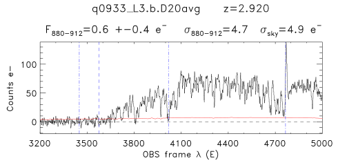
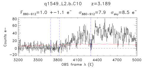
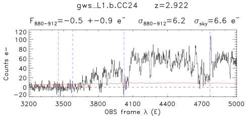
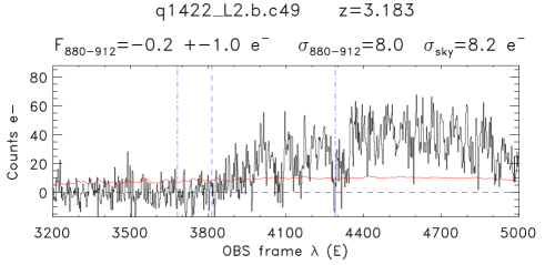
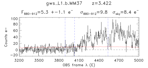
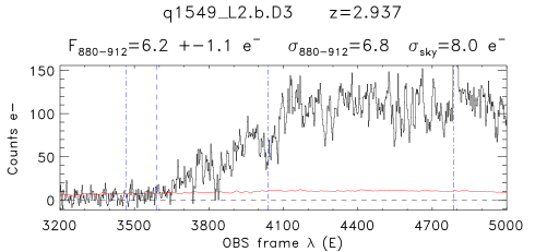
Figure 30.— Example extracted LRIS-B spectra, in units of mean photoelectrons per pixel prior to re-binning and flux calibration of the 1-D spectra. In each panel, the red curve is the 1$\sigma$ noise level per pixel expected from the noise model. The vertical lines in each panel mark, moving left to right, rest wavelengths 880, 912, 1026 ($Ly\beta$), and 1216 ($Ly\alpha$). The top left panel shows one of the two galaxies observed on 2 separate masks, after combining the independently reduced spectra in 1-D, with inverse-variance weighting. The annotations above each panel show the object name, redshift, mean and error in the mean of the number of photoelectrons per pixel over the [880,912] rest wavelength interval ($F_{880-912}$), the rms per pixel over the same range ($\sigma_{880-912}$), and the noise level per pixel expected over the same pixels based on the noise model in §A.5.1.

In evaluating the accuracy of our noise model, we examined each extracted 1-D spectrum after wavelength calibration, but prior to re-sampling in the dispersion direction or any other processing of the 1-D spectra and 1 $\sigma$ error arrays. These spectra, examples of which are shown in Figure 30, remain in units of raw photoelectrons summed over the 10 (spatial) pixel extraction aperture of the final 2-d background-subtracted stack, so that the spectrum is in units of electrons per wavelength pixel (1 pix $\simeq 2.14$ Å) averaged over typically 18 1800s exposures. Each panel in Figure 30 shows the mean and standard error in the mean e^- pix^-1 evaluated over the rest-frame [880,910] interval, $F_{880-912}$, the rms per pixel within that interval ($\sigma_{880-912}$), and the expected rms per pixel given by the background pixels and noise model described in §A.5.1 ($\sigma_{\rm sky}$). The top two rows (i.e. the first 4 spectra shown) are formal non-detections of LyC flux, and the bottom row shows two examples of formally detected objects (Westphal/GWS-MM37 and Q1549-D3). These examples illustrate that the predicted and measured noise levels in the spectral regions used for LyC measurement are very close to one another. Note that the top-left panel shows the combined spectrum of Q0933-D20 after averaging the 2 independent 1-D spectra with inverse variance weighting.

Appendix B Improved IGM Opacity Models for Galaxy Sources

Figure 31.— Distribution functions $f(N_{\rm HI},X)$ inferred from the H I absorber catalog of Rudie et al. (2013). The best-fit power law slopes $\beta$ for the “general IGM” (blue and black) and regions within 300 pkpc and $\delta v<700$ km s${}^{-1}\,$ from a galaxy in the observed galaxy sample (such regions include $\sim 7$% of the total effective survey volume; Rudie et al. 2012). The IGM has been divided into low-$N_{\rm HI}$ and high-$N_{\rm HI}$ subsamples at log ($N_{\rm HI}$/${\rm cm}^{-2})=15.2$ with separate slopes and normalizations allowed (Table 11). Note that the incidence of absorbers with log($N_{\rm HI}$/${\rm cm}^{-2})>16$ is $\sim 6$ times higher in the CGM of galaxies than in the general IGM (see text for discussion.)

For the purposes of generating Monte Carlo models of the IGM opacity, we adopted a combination of the measured $N_{\rm HI}$ distribution functions $f(N_{\rm HI},X)_{\rm IGM}$ and $f(N_{\rm HI},X)_{\rm CGM}$ as shown in Figure 31, both as presented by Rudie et al. (2013) based on data from the Keck Baryonic Structure Survey (KBSS). Here $f(N_{\rm HI},X)$ is the distribution function, first introduced by Carswell et al. (1984), describing the incidence of H I absorption systems per unit co-moving path length $X$, as defined by Bahcall & Peebles (1969). The parameter $X$ is cosmology-dependent, but for spatially flat CDM models it is given by

$$dX=\frac{H_{0}}{H(z)}(1+z)^{2}dz$$ (B1)

where

$$H(z)=H_{0}\left[\Omega_{\Lambda}+\Omega_{\rm m}(1+z)^{3}\right]^{1/2}$$ (B2)

is the Hubble parameter.

The CGM statistics (see Rudie et al. 2013) are derived based on measurements of $f(N_{\rm HI},X)$ for sightlines within 300 pkpc and $\pm 700$ km s${}^{-1}\,$ [$\Delta z\leq 0.0023(1+z_{\rm s})$] of spectroscopically-identified KBSS galaxies in the redshift range $2.0\lower 2.15277pt\hbox{$\;\buildrel<\over{\sim}\;$}z\lower 2.15277pt\hbox{$\;\buildrel<\over{\sim}\;$}2.8$. Aside from having somewhat lower redshift, the galaxies in KBSS were selected using very similar criteria to those of KLCS and occupy a nearly-identical range of stellar mass and star formation rate (see Adelberger et al. 2004; Steidel et al. 2004.) Figure 31 shows that within the CGM so-defined, the incidence of H I absorbers is $\sim 6$ times higher than the IGM average at the high-$N_{\rm HI}$ end of the $f(N_{\rm HI},X)$ distribution; for log $N_{\rm HI}$$\lower 2.15277pt\hbox{$\;\buildrel<\over{\sim}\;$}14$ the CGM regions asymptotically approach the statistics of the general IGM.

In general, $f(N_{\rm HI},X)$ is redshift-independent only if the physical properties of the absorbers do not evolve with redshift. Since the measurements in Rudie et al. (2013) are based on QSO sightlines with a path-length averaged redshift $\langle z\rangle=2.37$, we applied a redshift correction to the measured $f(N_{\rm HI},X)$ by expressing the number of absorbers of column density between $N_{\rm HI,min}$ and $N_{\rm HI,max}$ as

$$N_{\rm abs}=\int_{N_{\rm HI,min}}^{N_{\rm HI,max}}\int_{z1}^{z2}N_{\rm HI}^{-\beta}A(1+z)^{\gamma}dN_{\rm HI}dz$$ (B3)

where $N_{\rm abs}$ is the number of absorbers with $N_{\rm HI,min}<N_{\rm HI}<N_{\rm HI,max}$ expected over the redshift path interval $[z1,z2]$, $A$ is a constant chosen to match the observations at the effective redshift of the measured sample, $\beta$ is the slope of $f(N_{\rm HI},X)$, and $\gamma$ is a power law exponent describing the redshift evolution of the number of absorbers per unit redshift, $dN_{\rm abs}/dz\propto(1+z)^{\gamma}$.

For reasons discussed in detail by Rudie et al. (2013), we divided the full range of $N_{\rm HI}$ into two regimes: log $N_{\rm HI}$ $<15.2$ and log $N_{\rm HI}$ $>15.2$, with separate $\beta$, $\gamma$, and normalization $A$, as indicated in Figure 31. The values adopted for the MC simulations are summarized in Table 11.

Table 11Parameters for IGM/CGM Monte Carlo Simulations

	log($N_{\rm HI}$/${\rm cm}^{-2}$)	$\beta$	log($A$)	$\gamma$
IGM Low	$12.0-15.2$	$1.635$	9.305	2.50
IGM High	$15.2-21.0$	$1.463$	7.542	1.00
CGM	$13.0-21.0$	$1.381$	6.716	1.00

In the present case, our main interest is a quantitative estimate of the reduction in flux in a small wavelength range [880,910] Å in the rest-frame of a galaxy source. The effective flux decrement in this interval includes blanketing from Lyman series absorption lines – dominated by systems with log ($N_{\rm HI}$/cm${}^{-2})<15.2$) – and Lyman continuum opacity, dominated by higher $N_{\rm HI}$ systems at redshifts close to $z_{\rm s}$. Most of the line blanketing component is contributed by $\rm Ly\alpha$ and Ly$\beta$ falling at observed wavelengths near $900(1+z_{\rm s})$ Å. For example, at $z_{\rm s}=3.10$, the relevant redshifts are $z(\rm Ly\alpha)\simeq 1.97-2.07$ and $z({\rm Ly}\beta)\simeq 2.52-2.64$. This implies that the measurements of Rudie et al. (2013) require no extrapolation in redshift to accurately estimate the line opacity contribution to the transmission in the wavelength interval [880,910] in the rest frame for a source at $z_{\rm s}\simeq 3$. Rudie et al. (2013) verified that the overall incidence of the low-column density lines is consistent with $dN_{\rm abs}/dz\propto(1+z)^{2.5}$ for the $N_{\rm HI}$ range $12<{\rm log}N_{\rm HI}<15.2$, which has been assumed in our Monte Carlo realizations.

For Lyman continuum opacity, the most relevant absorption systems are those with $16<{\rm log(N_{\rm HI}/cm^{-2})}<18$ (Rudie et al. 2013) and redshifts within our chosen LyC interval of [880,910] in the source rest-frame, i.e., $z_{\rm s}-\Delta z\leq z\leq z_{\rm s}$, where $\Delta z=0.036(1+z_{\rm s})$. The LyC opacity depends on the higher $N_{\rm HI}$ portion of the distribution measured by Rudie et al. (2013), including systems with log ${\rm(N_{\rm HI}/cm^{-2})}>17.2$ (Lyman limit systems), which are not well sampled in that data set. However, Rudie et al. (2013) showed that the power-law extrapolation of $f(N_{\rm HI},X)$ to log ($N_{\rm HI}$/${\rm cm}^{-2})>17.2$ accurately reproduced the best available constraints on the incidence of Lyman limit systems (LLSs) at $z\sim 2.4$, and, assuming $\gamma=1.0$, at $z\sim 3$ as well. The point representing the LLSs (at ${\rm log~{}(N_{\rm HI}/cm^{-2})=17.7}$ in Figure 31 is the actual location of the data point for $17.2\leq{\rm log}N_{\rm HI}~{}\leq 18.2$ assuming the extrapolated slope and the observed total redshift path density of LLSs at $z\sim 3$. For the MC models, LLSs were drawn from a distribution that assumes $\beta=1.473$ over the full range $15.2\leq{\rm log}N_{\rm HI}\leq 21.0$.

Table 12Model IGM Transmission Versus Redshift

$z_{s}$	$\langle t_{900}\rangle$	10%	25%	50%	75%	90%	$\langle 1-D_{B}\rangle$
IGM Only
2.70	$0.516\pm 0.200$	0.175	0.417	0.588	0.663	0.708	$0.736\pm 0.028$
2.75	$0.504\pm 0.199$	0.160	0.398	0.571	0.654	0.698	$0.727\pm 0.028$
2.80	$0.486\pm 0.197$	0.148	0.376	0.554	0.634	0.680	$0.715\pm 0.027$
2.85	$0.478\pm 0.200$	0.143	0.368	0.550	0.630	0.671	$0.706\pm 0.028$
2.90	$0.469\pm 0.200$	0.138	0.347	0.543	0.622	0.661	$0.695\pm 0.030$
2.95	$0.461\pm 0.188$	0.136	0.346	0.524	0.602	0.646	$0.686\pm 0.028$
3.00	$0.446\pm 0.182$	0.133	0.332	0.506	0.584	0.631	$0.678\pm 0.028$
3.05	$0.432\pm 0.189$	0.127	0.311	0.496	0.580	0.626	$0.665\pm 0.028$
3.10	$0.435\pm 0.187$	0.123	0.325	0.488	0.569	0.616	$0.656\pm 0.027$
3.15	$0.417\pm 0.178$	0.116	0.304	0.471	0.557	0.605	$0.645\pm 0.029$
3.20	$0.402\pm 0.178$	0.095	0.294	0.461	0.537	0.588	$0.632\pm 0.028$
3.25	$0.390\pm 0.176$	0.091	0.278	0.452	0.533	0.575	$0.623\pm 0.028$
3.30	$0.377\pm 0.173$	0.089	0.259	0.425	0.513	0.560	$0.611\pm 0.027$
3.35	$0.363\pm 0.169$	0.085	0.242	0.416	0.502	0.545	$0.601\pm 0.029$
3.40	$0.345\pm 0.165$	0.078	0.230	0.393	0.488	0.527	$0.588\pm 0.025$
3.45	$0.344\pm 0.164$	0.069	0.223	0.382	0.482	0.522	$0.577\pm 0.028$
3.50	$0.322\pm 0.163$	0.053	0.198	0.362	0.456	0.501	$0.565\pm 0.027$
4.00	$0.226\pm 0.127$	0.034	0.117	0.244	0.332	0.383	$0.448\pm 0.025$
4.50	$0.147\pm 0.089$	0.012	0.069	0.155	0.219	0.262	$0.334\pm 0.022$
5.00	$0.088\pm 0.058$	0.006	0.036	0.088	0.137	0.164	$0.233\pm 0.017$
IGM+CGM
2.70	$0.454\pm 0.236$	0.021	0.276	0.540	0.643	0.694	$0.729\pm 0.030$
2.75	$0.439\pm 0.231$	0.019	0.249	0.517	0.633	0.680	$0.720\pm 0.029$
2.80	$0.422\pm 0.232$	0.015	0.241	0.500	0.611	0.661	$0.709\pm 0.028$
2.85	$0.412\pm 0.232$	0.013	0.208	0.489	0.609	0.660	$0.700\pm 0.028$
2.90	$0.397\pm 0.226$	0.014	0.214	0.466	0.587	0.645	$0.690\pm 0.030$
2.95	$0.392\pm 0.219$	0.013	0.209	0.462	0.578	0.636	$0.680\pm 0.030$
3.00	$0.371\pm 0.222$	0.012	0.175	0.431	0.561	0.622	$0.669\pm 0.030$
3.05	$0.369\pm 0.213$	0.012	0.189	0.427	0.550	0.609	$0.658\pm 0.030$
3.10	$0.352\pm 0.213$	0.011	0.135	0.393	0.529	0.589	$0.645\pm 0.031$
3.15	$0.347\pm 0.205$	0.012	0.170	0.405	0.522	0.577	$0.637\pm 0.028$
3.20	$0.326\pm 0.204$	0.010	0.137	0.366	0.502	0.572	$0.624\pm 0.029$
3.25	$0.321\pm 0.195$	0.009	0.150	0.353	0.489	0.552	$0.615\pm 0.029$
3.30	$0.321\pm 0.192$	0.006	0.147	0.359	0.485	0.543	$0.603\pm 0.029$
3.35	$0.310\pm 0.191$	0.003	0.141	0.351	0.474	0.531	$0.592\pm 0.030$
3.40	$0.291\pm 0.188$	0.002	0.119	0.315	0.459	0.516	$0.580\pm 0.030$
3.45	$0.272\pm 0.183$	0.002	0.094	0.303	0.427	0.498	$0.569\pm 0.030$
3.50	$0.264\pm 0.179$	0.002	0.100	0.302	0.434	0.492	$0.557\pm 0.029$
4.00	$0.196\pm 0.132$	0.001	0.074	0.204	0.311	0.365	$0.445\pm 0.025$
4.50	$0.115\pm 0.091$	0.000	0.026	0.109	0.191	0.245	$0.330\pm 0.022$
5.00	$0.068\pm 0.058$	0.000	0.010	0.064	0.115	0.152	$0.230\pm 0.017$

Monte Carlo realizations of IGM sightlines were made, using the same code as in Shapley et al. (2006) and Nestor et al. (2011) albeit with more detailed treatment of the higher-order Lyman series lines and with normalization parameters updated as in Table 11. The realizations include the full range $12<$log$N_{\rm HI}$ $<21$ drawn in a Poisson fashion according to the appropriate distribution function and redshift. Each realization for a given assumed source redshift $z_{\rm s}$ is a synthetic spectrum covering the observed wavelength range $3160-(1+z_{\rm s})1215.7$ Å. A set of 10,000 realizations at each of 17 assumed source redshifts (2.70-3.50 in steps of 0.05) was performed using the “IGM-only” version of $f(N_{\rm HI},X)$. Table 12 summarizes the results in terms of percentiles in transmission $t_{900}$, the mean unabsorbed fraction in the source rest-frame [880,910] interval. Also provided for each source redshift is the value of $\langle 1-D_{\rm B}\rangle$, where $D_{\rm B}$ is the mean flux decrement from Lyman line blanketing in the rest-frame interval [920,1015] (Oke & Korycansky 1982). As shown in §7, $\langle 1-D_{\rm B}\rangle$ is a close approximation to the maximum transmission expected in the [880,910] LyC interval at each value of $z_{\rm s}$, for sightlines without significant continuum opacity from high-$N_{\rm HI}$ absorbers.

As in Rudie et al. (2013), a second set of Monte Carlo realizations was made by drawing absorbers from the same IGM distribution $f(N_{\rm HI},X)_{\rm IGM}$, except within 700 km s${}^{-1}\,$[$\Delta z<0.0023(1+z_{\rm s})$]) of the source, where absorbers were instead drawn from the $f(N_{\rm HI},X)_{\rm CGM}$ distribution. This set of simulations is hereafter referred to as “IGM+CGM”; the statistics as a function of source redshift are summarized in the bottom half of Table 12.

References

- Adelberger et al. (2004) Adelberger, K. L., Steidel, C. C., Shapley, A. E., et al. 2004, ApJ, 607, 226, doi: 10.1086/383221
- Adelberger et al. (2003) Adelberger, K. L., Steidel, C. C., Shapley, A. E., & Pettini, M. 2003, ApJ, 584, 45
- Asplund et al. (2009) Asplund, M., Grevesse, N., Sauval, A. J., & Scott, P. 2009, ARA&A, 47, 481, doi: 10.1146/annurev.astro.46.060407.145222
- Bahcall & Peebles (1969) Bahcall, J. N., & Peebles, P. J. E. 1969, ApJ, 156, L7, doi: 10.1086/180337
- Becker & Bolton (2013) Becker, G. D., & Bolton, J. S. 2013, MNRAS, 436, 1023, doi: 10.1093/mnras/stt1610
- Becker et al. (2011) Becker, G. D., Bolton, J. S., Haehnelt, M. G., & Sargent, W. L. W. 2011, MNRAS, 410, 1096, doi: 10.1111/j.1365-2966.2010.17507.x
- Becker et al. (2015) Becker, G. D., Bolton, J. S., & Lidz, A. 2015, PASA, 32, e045, doi: 10.1017/pasa.2015.45
- Bershady et al. (1999) Bershady, M. A., Charlton, J. C., & Geoffroy, J. M. 1999, ApJ, 518, 103, doi: 10.1086/307257
- Borthakur et al. (2014) Borthakur, S., Heckman, T. M., Leitherer, C., & Overzier, R. A. 2014, Science, 346, 216, doi: 10.1126/science.1254214
- Bouwens et al. (2010) Bouwens, R. J., Illingworth, G. D., Oesch, P. A., et al. 2010, ApJ, 709, L133, doi: 10.1088/2041-8205/709/2/L133
- Bouwens et al. (2015) —. 2015, ApJ, 803, 34, doi: 10.1088/0004-637X/803/1/34
- Bridge et al. (2010) Bridge, C. R., Teplitz, H. I., Siana, B., et al. 2010, ApJ, 720, 465, doi: 10.1088/0004-637X/720/1/465
- Calzetti et al. (2000) Calzetti, D., Armus, L., Bohlin, R. C., et al. 2000, ApJ, 533, 682
- Cardamone et al. (2009) Cardamone, C., Schawinski, K., Sarzi, M., et al. 2009, MNRAS, 399, 1191, doi: 10.1111/j.1365-2966.2009.15383.x
- Carswell et al. (1984) Carswell, R. F., Morton, D. C., Smith, M. G., et al. 1984, ApJ, 278, 486, doi: 10.1086/161815
- Chisholm et al. (2018) Chisholm, J., Gazagnes, S., Schaerer, D., et al. 2018, ArXiv e-prints. https://arxiv.org/abs/1803.03655
- Choi et al. (2017) Choi, J., Conroy, C., & Byler, N. 2017, ApJ, 838, 159, doi: 10.3847/1538-4357/aa679f
- Cowie et al. (2009) Cowie, L. L., Barger, A. J., & Trouille, L. 2009, ApJ, 692, 1476, doi: 10.1088/0004-637X/692/2/1476
- de Barros et al. (2016) de Barros, S., Vanzella, E., Amorín, R., et al. 2016, A&A, 585, A51, doi: 10.1051/0004-6361/201527046
- Dijkstra et al. (2016) Dijkstra, M., Gronke, M., & Venkatesan, A. 2016, ApJ, 828, 71, doi: 10.3847/0004-637X/828/2/71
- Du et al. (2018) Du, X., Shapley, A. E., Reddy, N. A., et al. 2018, ArXiv e-prints. https://arxiv.org/abs/1803.05912
- Eldridge et al. (2017) Eldridge, J. J., Stanway, E. R., Xiao, L., et al. 2017, ArXiv e-prints. https://arxiv.org/abs/1710.02154
- Erb et al. (2012) Erb, D. K., Quider, A. M., Henry, A. L., & Martin, C. L. 2012, ApJ, 759, 26, doi: 10.1088/0004-637X/759/1/26
- Erb et al. (2014) Erb, D. K., Steidel, C. C., Trainor, R. F., et al. 2014, ApJ, 795, 33, doi: 10.1088/0004-637X/795/1/33
- Faucher-Giguère et al. (2008) Faucher-Giguère, C.-A., Lidz, A., Hernquist, L., & Zaldarriaga, M. 2008, ApJ, 682, L9, doi: 10.1086/590409
- Filippenko (1982) Filippenko, A. V. 1982, PASP, 94, 715, doi: 10.1086/131052
- Finkelstein et al. (2015) Finkelstein, S. L., Ryan, Jr., R. E., Papovich, C., et al. 2015, ApJ, 810, 71, doi: 10.1088/0004-637X/810/1/71
- Gazagnes et al. (2018) Gazagnes, S., Chisholm, J., Schaerer, D., et al. 2018, ArXiv e-prints. https://arxiv.org/abs/1802.06378
- Gordon et al. (2003) Gordon, K. D., Clayton, G. C., Misselt, K. A., Landolt, A. U., & Wolff, M. J. 2003, ApJ, 594, 279, doi: 10.1086/376774
- Grazian et al. (2016) Grazian, A., Giallongo, E., Gerbasi, R., et al. 2016, A&A, 585, A48, doi: 10.1051/0004-6361/201526396
- Grazian et al. (2017) Grazian, A., Giallongo, E., Paris, D., et al. 2017, A&A, 602, A18, doi: 10.1051/0004-6361/201730447
- Gronwall et al. (2007) Gronwall, C., Ciardullo, R., Hickey, T., et al. 2007, ApJ, 667, 79, doi: 10.1086/520324
- Hayashino et al. (2004) Hayashino, T., Matsuda, Y., Tamura, H., et al. 2004, AJ, 128, 2073, doi: 10.1086/424935
- Hayes et al. (2014) Hayes, M., Östlin, G., Duval, F., et al. 2014, ApJ, 782, 6, doi: 10.1088/0004-637X/782/1/6
- Heckman et al. (2011) Heckman, T. M., Borthakur, S., Overzier, R., et al. 2011, ApJ, 730, 5, doi: 10.1088/0004-637X/730/1/5
- Henry et al. (2015) Henry, A., Scarlata, C., Martin, C. L., & Erb, D. 2015, ApJ, 809, 19, doi: 10.1088/0004-637X/809/1/19
- Hopkins et al. (2007) Hopkins, P. F., Richards, G. T., & Hernquist, L. 2007, ApJ, 654, 731, doi: 10.1086/509629
- Inoue & Iwata (2008) Inoue, A. K., & Iwata, I. 2008, MNRAS, 387, 1681, doi: 10.1111/j.1365-2966.2008.13350.x
- Inoue et al. (2005) Inoue, A. K., Iwata, I., Deharveng, J.-M., Buat, V., & Burgarella, D. 2005, A&A, 435, 471, doi: 10.1051/0004-6361:20041769
- Inoue et al. (2014) Inoue, A. K., Shimizu, I., Iwata, I., & Tanaka, M. 2014, MNRAS, 442, 1805, doi: 10.1093/mnras/stu936
- Iwata et al. (2009) Iwata, I., Inoue, A. K., Matsuda, Y., et al. 2009, ApJ, 692, 1287, doi: 10.1088/0004-637X/692/2/1287
- Izotov et al. (2016a) Izotov, Y. I., Orlitová, I., Schaerer, D., et al. 2016a, Nature, 529, 178, doi: 10.1038/nature16456
- Izotov et al. (2016b) Izotov, Y. I., Schaerer, D., Thuan, T. X., et al. 2016b, MNRAS, 461, 3683, doi: 10.1093/mnras/stw1205
- Izotov et al. (2018) Izotov, Y. I., Schaerer, D., Worseck, G., et al. 2018, MNRAS, 474, 4514, doi: 10.1093/mnras/stx3115
- Jaskot & Oey (2013) Jaskot, A. E., & Oey, M. S. 2013, ApJ, 766, 91, doi: 10.1088/0004-637X/766/2/91
- Jaskot & Oey (2014) —. 2014, ApJ, 791, L19, doi: 10.1088/2041-8205/791/2/L19
- Jones et al. (2012) Jones, T., Stark, D. P., & Ellis, R. S. 2012, ApJ, 751, 51, doi: 10.1088/0004-637X/751/1/51
- Kornei et al. (2010) Kornei, K. A., Shapley, A. E., Erb, D. K., et al. 2010, ApJ, 711, 693, doi: 10.1088/0004-637X/711/2/693
- Law et al. (2007) Law, D. R., Steidel, C. C., Erb, D. K., et al. 2007, ApJ, 669, 929, doi: 10.1086/521786
- Law et al. (2011) Law, D. R., Steidel, C. C., Shapley, A. E., et al. 2011, ArXiv e-prints. https://arxiv.org/abs/1107.3137
- Le Fèvre et al. (2015) Le Fèvre, O., Tasca, L. A. M., Cassata, P., et al. 2015, A&A, 576, A79, doi: 10.1051/0004-6361/201423829
- Leitherer et al. (2014) Leitherer, C., Ekström, S., Meynet, G., et al. 2014, ApJS, 212, 14, doi: 10.1088/0067-0049/212/1/14
- Leitherer et al. (2016) Leitherer, C., Hernandez, S., Lee, J. C., & Oey, M. S. 2016, ApJ, 823, 64, doi: 10.3847/0004-637X/823/1/64
- Leitherer et al. (1999) Leitherer, C., Schaerer, D., Goldader, J. D., et al. 1999, ApJS, 123, 3
- Ma et al. (2016) Ma, X., Hopkins, P. F., Kasen, D., et al. 2016, MNRAS, 459, 3614, doi: 10.1093/mnras/stw941
- Madau (1995) Madau, P. 1995, ApJ, 441, 18, doi: 10.1086/175332
- Malkan et al. (2003) Malkan, M., Webb, W., & Konopacky, Q. 2003, ApJ, 598, 878, doi: 10.1086/379117
- Marchi et al. (2017a) Marchi, F., Pentericci, L., Guaita, L., et al. 2017a, A&A, 601, A73, doi: 10.1051/0004-6361/201630054
- Marchi et al. (2017b) —. 2017b, ArXiv e-prints. https://arxiv.org/abs/1710.10184
- Martin et al. (2012) Martin, C. L., Shapley, A. E., Coil, A. L., et al. 2012, ApJ, 760, 127, doi: 10.1088/0004-637X/760/2/127
- Massey et al. (1988) Massey, P., Strobel, K., Barnes, J. V., & Anderson, E. 1988, ApJ, 328, 315, doi: 10.1086/166294
- Matsuda et al. (2004) Matsuda, Y., Yamada, T., Hayashino, T., et al. 2004, AJ, 128, 569
- McLean et al. (2012) McLean, I. S., Steidel, C. C., Epps, H. W., et al. 2012, in Proc. SPIE, Vol. 8446, Ground-based and Airborne Instrumentation for Astronomy IV, 84460J
- Mostardi et al. (2013) Mostardi, R. E., Shapley, A. E., Nestor, D. B., et al. 2013, ApJ, 779, 65, doi: 10.1088/0004-637X/779/1/65
- Mostardi et al. (2015) Mostardi, R. E., Shapley, A. E., Steidel, C. C., et al. 2015, ApJ, 810, 107, doi: 10.1088/0004-637X/810/2/107
- Nakajima & Ouchi (2014) Nakajima, K., & Ouchi, M. 2014, MNRAS, 442, 900, doi: 10.1093/mnras/stu902
- Nestor et al. (2013) Nestor, D. B., Shapley, A. E., Kornei, K. A., Steidel, C. C., & Siana, B. 2013, ApJ, 765, 47, doi: 10.1088/0004-637X/765/1/47
- Nestor et al. (2011) Nestor, D. B., Shapley, A. E., Steidel, C. C., & Siana, B. 2011, ApJ, 736, 18, doi: 10.1088/0004-637X/736/1/18
- Oesch et al. (2010) Oesch, P. A., Bouwens, R. J., Carollo, C. M., et al. 2010, ApJ, 725, L150, doi: 10.1088/2041-8205/725/2/L150
- Oke & Korycansky (1982) Oke, J. B., & Korycansky, D. G. 1982, ApJ, 255, 11, doi: 10.1086/159797
- Oke et al. (1995) Oke, J. B., Cohen, J. G., Carr, M., et al. 1995, PASP, 107, 375
- Östlin et al. (2014) Östlin, G., Hayes, M., Duval, F., et al. 2014, ApJ, 797, 11, doi: 10.1088/0004-637X/797/1/11
- Overzier et al. (2009) Overzier, R. A., Heckman, T. M., Tremonti, C., et al. 2009, ApJ, 706, 203, doi: 10.1088/0004-637X/706/1/203
- Parsa et al. (2016) Parsa, S., Dunlop, J. S., McLure, R. J., & Mortlock, A. 2016, MNRAS, 456, 3194, doi: 10.1093/mnras/stv2857
- Pettini et al. (2002) Pettini, M., Rix, S. A., Steidel, C. C., et al. 2002, ApJ, 569, 742, doi: 10.1086/339355
- Phillips et al. (2006) Phillips, A. C., Miller, J., Cowley, D., & Wallace, V. 2006, in Proc. SPIE, Vol. 6269, Society of Photo-Optical Instrumentation Engineers (SPIE) Conference Series, 62691O
- Planck Collaboration et al. (2016) Planck Collaboration, Adam, R., Aghanim, N., et al. 2016, A&A, 596, A108, doi: 10.1051/0004-6361/201628897
- Prochaska et al. (2011) Prochaska, J. X., Kasen, D., & Rubin, K. 2011, ApJ, 734, 24, doi: 10.1088/0004-637X/734/1/24
- Prochaska et al. (2009) Prochaska, J. X., Worseck, G., & O’Meara, J. M. 2009, ApJ, 705, L113, doi: 10.1088/0004-637X/705/2/L113
- Quider et al. (2009) Quider, A. M., Pettini, M., Shapley, A. E., & Steidel, C. C. 2009, MNRAS, 398, 1263, doi: 10.1111/j.1365-2966.2009.15234.x
- Rakic et al. (2012) Rakic, O., Schaye, J., Steidel, C. C., & Rudie, G. C. 2012, ApJ, 751, 94, doi: 10.1088/0004-637X/751/2/94
- Reddy et al. (2010) Reddy, N. A., Erb, D. K., Pettini, M., Steidel, C. C., & Shapley, A. E. 2010, ApJ, 712, 1070, doi: 10.1088/0004-637X/712/2/1070
- Reddy et al. (2012) Reddy, N. A., Pettini, M., Steidel, C. C., et al. 2012, ApJ, 754, 25, doi: 10.1088/0004-637X/754/1/25
- Reddy & Steidel (2009) Reddy, N. A., & Steidel, C. C. 2009, ApJ, 692, 778, doi: 10.1088/0004-637X/692/1/778
- Reddy et al. (2008) Reddy, N. A., Steidel, C. C., Pettini, M., et al. 2008, ApJS, 175, 48, doi: 10.1086/521105
- Reddy et al. (2016a) Reddy, N. A., Steidel, C. C., Pettini, M., & Bogosavljević, M. 2016a, ApJ, 828, 107, doi: 10.3847/0004-637X/828/2/107
- Reddy et al. (2016b) Reddy, N. A., Steidel, C. C., Pettini, M., Bogosavljević, M., & Shapley, A. E. 2016b, ApJ, 828, 108, doi: 10.3847/0004-637X/828/2/108
- Reddy et al. (2015) Reddy, N. A., Kriek, M., Shapley, A. E., et al. 2015, ApJ, 806, 259, doi: 10.1088/0004-637X/806/2/259
- Reddy et al. (2017) Reddy, N. A., Oesch, P. A., Bouwens, R. J., et al. 2017, ArXiv e-prints. https://arxiv.org/abs/1705.09302
- Rivera-Thorsen et al. (2015) Rivera-Thorsen, T. E., Hayes, M., Östlin, G., et al. 2015, ApJ, 805, 14, doi: 10.1088/0004-637X/805/1/14
- Robertson et al. (2015) Robertson, B. E., Ellis, R. S., Furlanetto, S. R., & Dunlop, J. S. 2015, ApJ, 802, L19, doi: 10.1088/2041-8205/802/2/L19
- Rudie et al. (2013) Rudie, G. C., Steidel, C. C., Shapley, A. E., & Pettini, M. 2013, ApJ, 769, 146, doi: 10.1088/0004-637X/769/2/146
- Rudie et al. (2012) Rudie, G. C., Steidel, C. C., Trainor, R. F., et al. 2012, ApJ, 750, 67, doi: 10.1088/0004-637X/750/1/67
- Rutkowski et al. (2016) Rutkowski, M. J., Scarlata, C., Haardt, F., et al. 2016, ApJ, 819, 81, doi: 10.3847/0004-637X/819/1/81
- Scarlata & Panagia (2015) Scarlata, C., & Panagia, N. 2015, ApJ, 801, 43, doi: 10.1088/0004-637X/801/1/43
- Schlegel et al. (1998) Schlegel, D. J., Finkbeiner, D. P., & Davis, M. 1998, ApJ, 500, 525, doi: 10.1086/305772
- Shapley et al. (2003) Shapley, A. E., Steidel, C. C., Pettini, M., & Adelberger, K. L. 2003, ApJ, 588, 65
- Shapley et al. (2006) Shapley, A. E., Steidel, C. C., Pettini, M., Adelberger, K. L., & Erb, D. K. 2006, ApJ, 651, 688, doi: 10.1086/507511
- Shapley et al. (2016) Shapley, A. E., Steidel, C. C., Strom, A. L., et al. 2016, ApJ, 826, L24, doi: 10.3847/2041-8205/826/2/L24
- Siana et al. (2007) Siana, B., Teplitz, H. I., Colbert, J., et al. 2007, ApJ, 668, 62, doi: 10.1086/521185
- Siana et al. (2010) Siana, B., Teplitz, H. I., Ferguson, H. C., et al. 2010, ApJ, 723, 241, doi: 10.1088/0004-637X/723/1/241
- Siana et al. (2015) Siana, B., Shapley, A. E., Kulas, K. R., et al. 2015, ApJ, 804, 17, doi: 10.1088/0004-637X/804/1/17
- Songaila & Cowie (2010) Songaila, A., & Cowie, L. L. 2010, ApJ, 721, 1448, doi: 10.1088/0004-637X/721/2/1448
- Stark et al. (2010) Stark, D. P., Ellis, R. S., Chiu, K., Ouchi, M., & Bunker, A. 2010, MNRAS, 408, 1628, doi: 10.1111/j.1365-2966.2010.17227.x
- Steidel et al. (1998) Steidel, C. C., Adelberger, K. L., Dickinson, M., et al. 1998, ApJ, 492, 428, doi: 10.1086/305073
- Steidel et al. (2000) Steidel, C. C., Adelberger, K. L., Shapley, A. E., et al. 2000, ApJ, 532, 170, doi: 10.1086/308568
- Steidel et al. (2003) —. 2003, ApJ, 592, 728, doi: 10.1086/375772
- Steidel et al. (2011) Steidel, C. C., Bogosavljević, M., Shapley, A. E., et al. 2011, ApJ, 736, 160, doi: 10.1088/0004-637X/736/2/160
- Steidel et al. (2010) Steidel, C. C., Erb, D. K., Shapley, A. E., et al. 2010, ApJ, 717, 289, doi: 10.1088/0004-637X
- Steidel et al. (1996) Steidel, C. C., Giavalisco, M., Pettini, M., Dickinson, M., & Adelberger, K. L. 1996, ApJ, 462, L17, doi: 10.1086/310029
- Steidel et al. (2001) Steidel, C. C., Pettini, M., & Adelberger, K. L. 2001, ApJ, 546, 665
- Steidel et al. (2004) Steidel, C. C., Shapley, A. E., Pettini, M., et al. 2004, ApJ, 604, 534
- Steidel et al. (2016) Steidel, C. C., Strom, A. L., Pettini, M., et al. 2016, ApJ, 826, 159, doi: 10.3847/0004-637X/826/2/159
- Steidel et al. (2014) Steidel, C. C., Rudie, G. C., Strom, A. L., et al. 2014, ApJ, 795, 165, doi: 10.1088/0004-637X/795/2/165
- Strom et al. (2017) Strom, A. L., Steidel, C. C., Rudie, G. C., et al. 2017, ApJ, 836, 164, doi: 10.3847/1538-4357/836/2/164
- Trainor et al. (2015) Trainor, R. F., Steidel, C. C., Strom, A. L., & Rudie, G. C. 2015, ApJ, 809, 89, doi: 10.1088/0004-637X/809/1/89
- Trainor et al. (2016) Trainor, R. F., Strom, A. L., Steidel, C. C., & Rudie, G. C. 2016, ApJ, 832, 171, doi: 10.3847/0004-637X/832/2/171
- Turner et al. (2014) Turner, M. L., Schaye, J., Steidel, C. C., Rudie, G. C., & Strom, A. L. 2014, MNRAS, 445, 794, doi: 10.1093/mnras/stu1801
- Vanzella et al. (2010) Vanzella, E., Giavalisco, M., Inoue, A. K., et al. 2010, ApJ, 725, 1011, doi: 10.1088/0004-637X/725/1/1011
- Vanzella et al. (2012) Vanzella, E., Guo, Y., Giavalisco, M., et al. 2012, ApJ, 751, 70, doi: 10.1088/0004-637X/751/1/70
- Vanzella et al. (2015) Vanzella, E., de Barros, S., Castellano, M., et al. 2015, A&A, 576, A116, doi: 10.1051/0004-6361/201525651
- Vanzella et al. (2017) Vanzella, E., Nonino, M., Cupani, G., et al. 2017, ArXiv e-prints. https://arxiv.org/abs/1712.07661
- Vasei et al. (2016) Vasei, K., Siana, B., Shapley, A. E., et al. 2016, ApJ, 831, 38, doi: 10.3847/0004-637X/831/1/38
- Verhamme et al. (2015) Verhamme, A., Orlitová, I., Schaerer, D., & Hayes, M. 2015, A&A, 578, A7, doi: 10.1051/0004-6361/201423978
- Verhamme et al. (2017) Verhamme, A., Orlitová, I., Schaerer, D., et al. 2017, A&A, 597, A13, doi: 10.1051/0004-6361/201629264
- Wise & Cen (2009) Wise, J. H., & Cen, R. 2009, ApJ, 693, 984, doi: 10.1088/0004-637X/693/1/984
- Wisotzki et al. (2016) Wisotzki, L., Bacon, R., Blaizot, J., et al. 2016, A&A, 587, A98, doi: 10.1051/0004-6361/201527384
- Wyithe & Cen (2007) Wyithe, J. S. B., & Cen, R. 2007, ApJ, 659, 890, doi: 10.1086/511948
- Yajima et al. (2014) Yajima, H., Li, Y., Zhu, Q., et al. 2014, MNRAS, 440, 776, doi: 10.1093/mnras/stu299
- Zackrisson et al. (2013) Zackrisson, E., Inoue, A. K., & Jensen, H. 2013, ApJ, 777, 39, doi: 10.1088/0004-637X/777/1/39