Martin boundaries of representations of the Cuntz algebra

Abstract.

In a number of recent papers, the idea of generalized boundaries has found use in fractal and in multiresolution analysis; many of the papers having a focus on specific examples. Parallel with this new insight, and motivated by quantum probability, there has also been much research which seeks to study fractal and multiresolution structures with the use of certain systems of non-commutative operators; non-commutative harmonic/stochastic analysis. This in turn entails combinatorial, graph operations, and branching laws. The most versatile, of these non-commutative algebras are the Cuntz algebras; denoted $\mathcal{O}_{N}$, $N$ for the number of isometry generators. $N$ is at least 2. Our focus is on the representations of $\mathcal{O}_{N}$. We aim to develop new non-commutative tools, involving both representation theory and stochastic processes. They serve to connect these parallel developments.

In outline, boundaries, Poisson, or Martin, are certain measure spaces (often associated to random walk models), designed to encode the asymptotic behavior, e.g., how trajectories diverge when the number of steps goes to infinity. We stress that our present boundaries (commutative or non-commutative) are purely measure-theoretical objects. Although, as we show, in some cases our boundaries may be compared with more familiar topological boundaries.

1. Introduction

We propose a new notion of Martin boundary for representations of the Cuntz algebras. It bridges two ideas which have been studied extensively in the literature, but so far have not been connected in a systematic fashion. In summary, they are: (i) the non-commutativity of the Cuntz algebras (see, e.g., [Cun77, BJ02, BJOk04]), and the subtleties of their representations [Gli60, Gli61], on the one hand; and (ii) symbolic representations of Markov chains and their classical Martin boundaries, on the other (see, e.g., [JT15, SBM07, Kor08, Tak11]). Applications include an harmonic analysis of iterated function system (IFS) measures. (See [Sto13, Rug16, MU15, JR05, Rue04, Pap15].)

In the study of representations of $\mathcal{O}_{N}$ on a Hilbert space $\mathscr{H}$, an identification of suitably closed invariant subspaces of $\mathscr{H}$ plays a central role. Here we refer to a representation in the form of a system operators $S_{i}$ and their adjoints $S_{i}^{*}$ satisfying the Cuntz relations. Of the possibilities for subspaces, invariance under the $S_{i}^{*}$ operators is more interesting: i.e., invariance under a system of generalized backwards shifts. In many cases, these invariant subspaces have small dimension, and they help us define new isomorphism invariants for the representations under discussion. For example, a permutative representation is one with the property that the vectors in some choice of ONB are permuted by the $S_{i}^{*}$ operators. Moreover, in important applications to quantum statistical mechanics, certain subspaces of states that are invariant under the adjoints $S_{i}^{*}$, are often finite-dimensional. They are called finitely correlated states. And they are one of the main features of interest in statistical mechanics, see e.g., [FNW92, FNW94, BJ97, Mat98, Ohn07, BJKW00]. They are analogues of “attractors” in classical (commutative) symbolic dynamics.

As we show in Section 5 in the present paper, there is a way to associate families of representations of the Cuntz algebras to a certain analyses of iterated function systems (IFSs), and for this reason, some of the earlier work on IFSs is relevant to our present considerations. For this part of the literature, we refer the reader to the papers [JLW12, LN14, KLW17, LN12, Vee12, EGW17, FGJ⁺17, FGJ⁺18b, FGJ⁺18a], and the papers cited there.

2. Preliminaries

We begin with a technical lemma regarding projections in Hilbert space; to be used inside the arguments throughout the paper.

Let $\mathscr{H}$ be a Hilbert space. By an orthogonal projection $P$ on $\mathscr{H}$, we mean an operator satisfying $P=P^{*}=P^{2}$. There is a bijective correspondence between projections $P$ (we shall assume that $P$ is orthogonal even if not stated) on the one hand, and closed subspaces $\mathscr{F}=\mathscr{F}_{P}$ in $\mathscr{H}$ on the other, given by $\mathscr{F}=P\mathscr{H}$; see e.g., [JT17].

We shall use the following

Lemma 2.1.

Let $P$ and $Q$ be projections, and let $\mathscr{F}_{P}$ and $\mathscr{F}_{Q}$ be the corresponding closed subspaces, then TFAE:

1. $P=PQ$;

2. $P=QP$;

3. $\mathscr{F}_{P}\subseteq\mathscr{F}_{Q}$;

4. $\left\|Ph\right\|\leq\left\|Qh\right\|$, $\forall h\in\mathscr{H}$;

5. $\left\langle h,Ph\right\rangle\leq\left\langle h,Qh\right\rangle$, $\forall h\in\mathscr{H}$.

When the conditions hold we say that $P\leq Q$.

Proof.

This is standard in operator theory. We refer to [JT17] for details. ∎

Definition 2.2.

1. Let $\mathscr{H}$ be a Hilbert space, and $V$ an operator in $\mathscr{H}$. If $P:=V^{*}V$ is a projection, we say that $V$ is a partial isometry. In that case, $Q=VV^{*}$ is also a projection: We say that $P$ is the initial projection of $V$, and that $Q$ is the final projection.

2. If $\mathfrak{A}$ is a $C^{*}$-algebra, and $V$, $P$, $Q$ are as above. If $V$ is in $\mathfrak{A}$, then we say that the two projections $P$ and $Q$ are $\mathfrak{A}$-equivalent.

Lemma 2.3.

Let $\left\{P_{k}\right\}_{k\in\mathbb{N}}$ be monotone, i.e.,

$$P_{1}\leq P_{2}\leq\cdots,$$ (2.1)

then the limit

$$P_{\infty}:=\lim_{k\rightarrow\infty}P_{k}$$ (2.2)

$($in the strong operator topology of $\mathscr{B}\left(\mathscr{H}\right)$$)$ exists, and $P_{\infty}$ is the projection onto the closed span of the subspaces $\left\{\mathscr{F}_{P_{k}}\right\}_{k\in\mathbb{N}}$.

The analogous conclusion holds for monotone decreasing sequence of projections

$$\cdots\leq Q_{n+1}\leq Q_{n}\leq\cdots\leq Q_{2}\leq Q_{1}.$$ (2.3)

In this case

$$Q_{\infty}=\lim_{k\rightarrow\infty}Q_{k}$$ (2.4)

is the projection onto $\bigcap_{k}\mathscr{F}_{Q_{k}}$.

3. A Projection Valued Random Variable

The theme of our paper falls at the crossroads of representation theory and the study of fractal measures and their stochastic processes.

The past two decades has seen a burst of research dealing with representations of classes of infinite $C^{*}$-algebras, which includes the Cuntz algebras [Cun77], $\mathcal{O}_{N}$ (see (3.5)) as well as other graph-$C^{*}$-algebras [FGJ⁺17, FGJ⁺18b]. (For details on a number of such earlier studies and applications, readers are referred to the papers cited below.) A source of motivation for our present work includes more recent research which includes both pure and applied mathematics: branching laws for endomorphisms, subshifts, endomorphisms from measurable partitions, Markov measures and topological Markov chains, wavelets and multiresolutions, signal processing and filters, iterated function systems (IFSs) and fractals, complex projective spaces, quasi-crystals, orbit equivalence, and substitution dynamical systems, and tiling systems [AJ15, JT15, AJL17, JT17, AJL18].

A projection $P$ is said to be infinite iff (Def) it contains proper subprojections, say $Q$, $Q\lneqq P$, such that $P$ and $Q$ are equivalent; (see Definition 2.2 (ii)). The Cuntz algebras $\mathcal{O}_{N}$ contain infinite projections; see Sections 4-5.

The questions considered here for representations of the Cuntz algebras are of independent interest as part of non-commutative harmonic analysis, i.e., the study of representations of non-abelian groups and $C^{*}$-algebras. A basic question in representation theory is that of determining parameters for the equivalence classes of representations, where “equivalence” refers to unitary equivalence. Since analysis and synthesis of representations must entail direct integral decompositions, a minimal requirement for a list of parameters for the equivalence classes of representations, is that it be Borel. When such a choice is possible, we say that there is a Borel cross section for the representations under consideration.

A pioneering paper by J. Glimm [Gli60] showed that there are infinite $C^{*}$-algebras whose representations do not have Borel cross sections. (Loosely speaking, the representations do not admit classification.) It is known that the Cuntz algebras, and $C^{*}$-algebras of higher-rank graphs, fall in this class. Hence, the approach to representations must narrow to suitable and amenable classes of representations which arise naturally in applications, and which do admit Borel cross sections.

A leading theme in our paper is a formulation of a boundary theory for representations of the Cuntz algebra. This in turn ties in with multiresolutions and with iterated function system (IFS) measures. A boundary theory for the latter has recently been suggested in various special cases.

A multiresolution approach to the study of representations of the Cuntz algebras was initiated by the first named author and O. Brattelli [BJKR01, BJKR02, BJ02, BJOk04]; and it includes such applications as construction of new multiresolution wavelets, and of wavelet algorithms from multi-band wavelet filters. And yet other applications studied by the first named author and D. Dutkay lead to the study of such classes of representations as monic, and permutative [DJ14, FGJ⁺18a]; and their use in fractal analysis. The introduction of these classes begins with the fact that every representation of the Cuntz algebra corresponds in a canonical fashion to a certain projection valued measure. We begin with these projection valued measures in this and the next section below.

Let $N$ be a positive integer, and let $A$ be an alphabet with $\left|A\right|=N$; set

$$\Omega_{N}:=A^{\mathbb{N}}=\underset{\aleph_{0}-\text{infinite Cartesian product}}{\underbrace{A\times A\times A\times\cdots\cdots\cdots}}.$$ (3.1)

Points in $\Omega_{N}$ are denoted $\omega:=\left(x_{1},x_{2},\cdots\right)$, and we set

$$\pi_{n}\left(\omega\right):=x_{n},\quad\forall\omega\in\Omega_{N}.$$ (3.2)

When $k\in\mathbb{N}$ is fixed, and $\omega=\left(x_{i}\right)\in\Omega_{N}$, we set

$$\omega|_{k}=\left(x_{1},x_{2},\cdots,x_{k}\right)=\text{the $k$-truncated (\emph{finite}) word.}$$ (3.3)

Let $\mathscr{H}$ be a separable Hilbert space, $\dim\mathscr{H}=\aleph_{0}$, and let $\mathfrak{M}$ be a commutative family of orthogonal projections in $\mathscr{H}$.

By an $\mathfrak{M}$-valued random variable $X$, we mean a measurable function

$$X:\Omega_{N}\longrightarrow\mathfrak{M}.$$ (3.4)

See, e.g., [AJ15, AJL17, AJL18].

Let $\mathcal{O}_{N}$ denote the Cuntz algebra with $N$ generators [Cun77], i.e., the $C^{*}$-algebra on symbols $\left\{s_{i}\right\}_{i=1}^{N}$, satisfying the following two relations:

$$s_{i}^{*}s_{j}=\delta_{ij}\mathbbm{1},\quad\text{and}\quad\sum_{i=1}^{N}s_{i}s_{i}^{*}=\mathbbm{1},$$ (3.5)

where $\mathbbm{1}$ denotes the unit element in $\mathcal{O}_{N}$.

By a representation of $\mathcal{O}_{N}$ we mean a function $s_{i}\mapsto S_{i}=\pi\left(s_{i}\right)$ such that

$$S_{i}^{*}S_{j}=\delta_{ij}I,\quad\text{and}\quad\sum_{i=1}^{N}S_{i}S_{i}^{*}=I$$ (3.6)

where $\delta_{ij}$ denotes the Kronecker delta, and $I$ denotes the identity operator in $\mathscr{H}$; we say that $\pi\in Rep\left(\mathcal{O}_{N},\mathscr{H}\right)$ if (3.6) holds.

The following lemma is basic and will be used throughout in the remaining of the paper.

Lemma 3.1.

Let $\pi=\left(S_{i}\right)_{i=1}^{N}$ be a representation of $\mathcal{O}_{N}$ acting in a fixed Hilbert space $\mathscr{H}$, i.e., $\pi\in Rep\left(\mathcal{O}_{N},\mathscr{H}\right)$. For finite words $f=\left(x_{1},\cdots,x_{n}\right)$ in the alphabet $A=\left\{1,2,\cdots,N\right\}$, set

$$P_{f}:=S_{x_{1}}S_{x_{2}}\cdots S_{x_{k}}S_{x_{k}}^{*}S_{x_{k-1}}^{*}\cdots S_{x_{1}}^{*}$$ (3.7)

with the conventions:

$$P_{i}:=S_{i}S_{i}^{*},\quad\text{and}\quad P_{\emptyset}=0.$$ (3.8)

1. Then as $f$ varies over all finite non-empty words, the projections $\left\{P_{f}\right\}$ form an abelian family.

2. Moreover,

   $$\sum_{i=1}^{N}P_{\left(fi\right)}=P_{f},$$ (3.9)

   and in particular,

   $$P_{\left(fg\right)}\leq P_{f}$$ (3.10)

   for any pair of finite non-empty words $f$ and $g$. Here $\left(fg\right)$ denotes concatenation of the two words.

Proof.

This is an application of (3.6), and the details are left for the reader. ∎

Theorem 3.2.

Let $N$, $\mathscr{H}$, $\mathcal{O}_{N}$, and $\pi\in Rep\left(\mathcal{O}_{N},\mathscr{H}\right)$ be as above.

1. Then there is a unique random variable $X$ (projection-valued, see (3.4)) such that

   $$X\left(\omega\right)=\lim_{k\rightarrow\infty}S_{\omega|_{k}}S_{\omega|_{k}}^{*},\;\omega\in\Omega_{N},$$ (3.11)

   where

   $$S_{\omega|_{k}}=S_{x_{1}}S_{x_{2}}\cdots S_{x_{k}}$$ (3.12)

   and $\omega|_{k}$ is the corresponding truncated word as in (3.3).

1. Moreover, the following relations hold:

   If $a\in A$, and $\omega=\left(x_{1},x_{2},x_{3},x_{4},\cdots\right)\in\Omega_{N}$, then

   $$S_{a}X\left(\omega\right)S_{a}^{*} =X\left(a\omega\right),$$ (3.13)

   and

   $$S_{a}^{*}X\left(\omega\right)S_{a}=\delta_{a,\pi_{1}\left(\omega\right)}X\left(\sigma\left(\omega\right)\right),$$ (3.14)

   where

   $$\sigma\left(\omega\right)=\left(x_{2},x_{3},x_{4},\cdots\right),\;\text{and}\quad a\omega=\left(a,x_{1},x_{2},x_{3},x_{4},\cdots\right).$$

2. Finally, we have:

   $$X\left(\omega\right)X\left(\omega^{\prime}\right)=\delta_{\omega,\omega^{\prime}}X\left(\omega\right),$$ (3.15)

   for all $\omega,\omega^{\prime}\in\Omega_{N}$.

Proof.

Let $N\in\mathbb{N}$, $N\geq 2$, and let $\mathscr{H}$ be a separable Hilbert space. Let $\mathcal{O}_{N}$ denote the Cuntz algebra with $N$ generators $\left\{s_{i}\right\}_{1}^{N}$, and let $\pi\in Rep\left(\mathcal{O}_{N},\mathscr{H}\right)$, $\pi\left(s_{i}\right):=S_{i}$, $1\leq i\leq N$, be fixed.

Let $\Omega_{N}$ be as in (3.1). For $\omega=\left(i_{1},i_{2},i_{3},\cdots\right)\in\Omega_{N}$, and $k\in\mathbb{N}$, set $\omega|_{k}=\left(i_{1},i_{2},\cdots,i_{k}\right)$, the truncated word; see (3.3). Set $S_{\omega|_{k}}=S_{i_{1}}\cdots S_{i_{k}}$, and

$$P\left(\omega|_{k}\right):=S_{\omega|_{k}}S_{\omega|_{k}}^{*}.$$ (3.16)

Then $\left\{P\left(\omega|_{k}\right)\right\}_{k\in\mathbb{N}}$ in (3.16) is a monotone decreasing family of projections, i.e.,

$$P\left(\omega|_{1}\right)\geq P\left(\omega|_{2}\right)\geq\cdots\geq P\left(\omega|_{k}\right)\geq P\left(\omega|_{k+1}\right)\geq\cdots;$$ (3.17)

and so, by Lemma 2.3, the following limit projection exists:

$$X\left(\omega\right):=\lim_{k\rightarrow\infty}P\left(\omega|_{k}\right).$$

Specifically, the limit exists in the strong operator topology on $\mathscr{B}\left(\mathscr{H}\right)$, and $X\left(\omega\right)$ is the projection onto the intersection of the closed subspaces in $\mathscr{H}$ given by

$$S_{\omega|_{k}}\mathscr{H}=S_{i_{1}}S_{i_{2}}\cdots S_{i_{k}}\mathscr{H}$$

as $k$ varies over $\mathbb{N}$.

The proof of monotonicity in (3.17) is the following estimate in the order of projections (see Lemma 2.1):

$$\underset{P\left(\omega|_{k+1}\right)}{\underbrace{S_{i_{1}}\cdots S_{i_{k}}S_{i_{k+1}}S_{i_{k+1}}^{*}S_{i_{k}}^{*}\cdots S_{i_{1}}^{*}}}\leq\underset{P\left(\omega|_{k}\right)}{\underbrace{S_{i_{1}}\cdots S_{i_{k}}S_{i_{k}}^{*}\cdots S_{i_{1}}^{*}}}.$$

See also Lemma 3.1. Once the limits are established, conclusion (i) in the theorem is clear.

The remaining conclusions (ii)-(iii) follow from passing to the limit $k\rightarrow\infty$ as follows. Here $\omega,\omega^{\prime}\in\Omega_{N}$ are fixed infinite words, $\omega=\left(i_{1},i_{2},i_{3},\cdots\right)$, $\omega^{\prime}=\left(j_{1},j_{2},j_{3},\cdots\right)$, and let $a\in A=\left\{1,2,\cdots,N\right\}$.

Conclusion (3.13) follows from:

$$S_{a}S_{i_{1}}\cdots S_{i_{k}}S_{i_{k}}^{*}\cdots S_{i_{1}}^{*}S_{a}^{*}=S_{a\omega|_{k}}S_{a\omega|_{k}}^{*},$$

and then passing to the limit, $k\rightarrow\infty$, using (i).

Conclusion (3.14) follows from

$$S_{a}^{*}S_{i_{1}}\cdots S_{i_{k}}S_{i_{k}}^{*}\cdots S_{i_{1}}^{*}S_{a}=\delta_{a,i_{1}}S_{i_{2}}\cdots S_{i_{k}}S_{i_{k}}^{*}\cdots S_{i_{2}}^{*}.$$

Here we used (3.6), since $\pi$ is given to be in $Rep\left(\mathcal{O}_{N},\mathscr{H}\right)$. Now (3.14) follows from taking the limit $k\rightarrow\infty$, and using again Lemma 2.3.

Finally, conclusion (iii) in the theorem follows from the computation:

$$S_{i_{1}}\cdots S_{i_{k}}\left(S_{i_{k}}^{*}\cdots S_{i_{1}}^{*}S_{j_{1}}\cdots S_{j_{k}}\right)S_{j_{k}}^{*}\cdots S_{j_{1}}^{*}=\delta_{i_{1}j_{1}}\delta_{i_{2}j_{2}}\cdots\delta_{i_{k}j_{k}}S_{i_{1}}\cdots S_{i_{k}}S_{i_{k}}^{*}\cdots S_{i_{1}}^{*}.$$

Passing to the limit $k\rightarrow\infty$, the desired conclusion (iii) now follows. ∎

4. A Projection Valued Path-Space Measure

Let $\mathscr{H}$ be a separable Hilbert space, and fix $N\geq 2$, and $\pi\in Rep\left(\mathcal{O}_{N},\mathscr{H}\right)$. We shall be concerned with two tools directly related to the study of representations of $\mathcal{O}_{N}$ on $\mathscr{H}$. (Also see [Mey93, Jor07, BKW12].)

With $\pi\left(s_{i}\right)=S_{i}$, $1\leq i\leq N$ fixed, set $\beta=\beta_{\pi}\in End\left(\mathscr{B}\left(\mathscr{H}\right)\right)$, endomorphism, and $\mathbb{Q}=\mathbb{Q}_{\pi}$, a canonical projection-valued path-space measure. Before giving the precise details, we shall need a few facts about the path space,

$$\Omega_{N}=\left\{1,2,\cdots,N\right\}^{\mathbb{N}}.$$ (4.1)

This version of path-space is chosen for simplicity: We have taken as alphabet the set $A:=\left\{1,2,\cdots,N\right\}$, but the fixed alphabet could be any finite set $A$ with $\left|A\right|=N$; and so $\Omega_{N}=A^{\mathbb{N}}=\underset{\aleph_{0}}{\underbrace{A\times A\times\cdots}}$, the infinite Cartesian product; see Section 2.

Definition 4.1.

For $T\in\mathscr{B}\left(\mathscr{H}\right)$, set

$$\beta_{\pi}\left(T\right)=\sum_{i=1}^{N}S_{i}TS_{i}^{*}.$$ (4.2)

Then $\beta_{\pi}\in End\left(\mathscr{B}\left(\mathscr{H}\right)\right)$, i.e.,

$$\beta_{\pi}\left(TT^{\prime}\right) =\beta_{\pi}\left(T\right)\beta_{\pi}\left(T^{\prime}\right),\;\forall T,T^{\prime}\in\mathscr{B}\left(\mathscr{H}\right);$$ (4.3)

$$\beta_{\pi}\left(T^{*}\right) =\beta_{\pi}\left(T\right)^{*},\;\text{and}$$ (4.4)

$$\beta_{\pi}\left(I\right) =I.$$ (4.5)

Given a representation $\pi\in Rep\left(\mathcal{O}_{N},\mathscr{H}\right)$, then the corresponding endomorphism,

$$\beta_{\pi}:\mathscr{B}\left(\mathscr{H}\right)\longrightarrow\mathscr{B}\left(\mathscr{H}\right)$$ (4.6)

plays an important role in representation theory. For example, for decompositions of $\pi$, by Schur, we will need the commutant $\left\{\pi\right\}^{\prime}$, defined as follows:

$$\left\{\pi\right\}^{\prime}:=\left\{T\in\mathscr{B}\left(\mathscr{H}\right)\mathrel{{;}}T\,\pi\left(A\right)=\pi\left(A\right)T,\;\forall A\in\mathcal{O}_{N}\right\}.$$ (4.7)

Lemma 4.2.

Let $\pi$ and $\beta_{\pi}$ be as in (4.2) and (4.6); then

$$\left\{\pi\right\}^{\prime}=\left\{T\in\mathscr{B}\left(\mathscr{H}\right)\mathrel{{;}}\beta_{\pi}\left(T\right)=T\right\}\left(=\text{Fix}\left(\beta_{\pi}\right).\right)$$ (4.8)

Proof.

We have the following bi-implications:

$$\beta_{\pi}\left(T\right) = T$$

$$\Updownarrow$$

$$S_{i}^{*}\beta_{\pi}\left(T\right) = S_{i}^{*}T,\quad 1\leq i\leq N$$

$$\Updownarrow \left(\text{by $\left(\ref{eq:e2}\right)$}\right)$$

$$TS_{i}^{*} = S_{i}^{*}T,\quad 1\leq i\leq N$$

$$\Updownarrow$$

$$T \in \left\{\pi\right\}^{\prime}.$$

∎

In applications to statistical mechanics, given $\pi\in Rep\left(\mathcal{O}_{N},\mathscr{H}\right)$, it is important to determine the closed subspaces $\mathscr{K}\subset\mathscr{H}$, invariant under the operators $S_{i}^{*}$, $1\leq i\leq N$.

Notation: When $\mathscr{K}$ is a closed subspace, we shall denote the corresponding projection by $P\left(=P_{\mathscr{K}}\right)$ (see Lemma 2.1.)

Lemma 4.3.

Let $\left(\pi,\mathscr{H},\mathscr{K}\left(\text{with projection }P\right)\right)$ be as above; then TFAE:

1. $S_{i}^{*}\mathscr{K}\subseteq\mathscr{K}$, $1\leq i\leq N$;

2. $PS_{i}^{*}P=S_{i}^{*}P$, $1\leq i\leq N$;

3. $P\leq\beta_{\pi}\left(P\right)$, in the order of projections (see Section 2); and

4. $P\leq\beta_{\pi}\left(P\right)\leq\cdots\leq\beta_{\pi}^{k}\left(P\right)\leq\beta_{\pi}^{k+1}\left(P\right)\leq\cdots$.

Proof.

The argument is the same as that used in the proof of Lemma 4.2. ∎

Lemma 4.4.

Let $\left(\pi,\mathscr{H},\mathscr{K}\left(\text{with projection }P\right)\right)$ be as in Lemma 4.3, and set

$$Q=\bigvee_{k=1}^{\infty}\beta_{\pi}^{k}\left(P\right);$$ (4.9)

then $Q\in\left\{\pi\right\}^{\prime}$, and $Q$ is the smallest projection in $\left\{\pi\right\}^{\prime}$ satisfying $P\leq Q$.

Proof.

The conclusion is immediate from the formula:

$$S_{i}^{*}\beta_{\pi}^{k+1}\left(P\right)=\beta_{\pi}^{k}\left(P\right)S_{i}^{*},\;1\leq i\leq N.$$

Assuming (4.9), we then get

$$S_{i}^{*}Q=QS_{i}^{*},\;1\leq i\leq N,$$

and by taking adjoints

$$QS_{i}=S_{i}Q;$$

so $Q\in\left\{\pi\right\}^{\prime}$. The remaining parts of the proof are immediate. ∎

Definition 4.5.

We shall use the standard $\sigma$-algebra $\mathscr{C}$ of subsets of $\Omega_{N}$ (the path-space). The $\sigma$-algebra is generated by cylinder sets $E_{f}$. Here $f=\left(i_{1},i_{2},\cdots,i_{k}\right)$ is a finite word, $\left|f\right|=k$; and

$$E_{f}:=\left\{\omega\in\Omega_{N}\mid\omega_{j}=i_{j},\;1\leq j\leq k\right\};$$ (4.10)

is one of the basic cylinder sets (see Fig 4.1). The $\sigma$-algebra $\mathscr{C}$ is the smallest $\sigma$-algebra containing the sets $E_{f}$ as $f$ varies over all finite words in the fixed alphabet $A$.

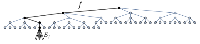
Figure 4.1. A basic cylinder set.

Definition 4.6 (Operators on path-space).

We recall the shift operators on $\Omega_{N}$, as follows: If $\omega=\left(i_{1},i_{2},i_{3},\cdots\right)\in\Omega_{N}$ , set

$$\sigma\left(\omega\right) :=\left(i_{2},i_{3},i_{4},\cdots\right),\;\text{and}$$ (4.11)

$$\hat{\tau}_{j}\left(\omega\right) :=\left(j,i_{1},i_{2},i_{3},\cdots\right).$$ (4.12)

If $E\subset\Omega_{N}$ is a subset, and $f$ is a finite word, we set

$$\sigma\left(E\right) =\left\{\sigma\left(\omega\right)\mid\omega\in E\right\},$$ (4.13)

$$\hat{\tau}_{j}\left(E\right) =\left\{\hat{\tau}_{j}\left(\omega\right)\mid\omega\in E\right\},$$ (4.14)

$$\sigma^{-1}\left(E\right) =\left\{\omega\in\Omega_{N}\mid\sigma\left(\omega\right)\in E\right\},\;\text{and}$$ (4.15)

$$fE =\big{\{}\underbrace{f\omega}\mid\omega\in E\big{\}}$$ (4.16)

$$\qquad\text{concatination of words}.$$

Note

$$\sigma^{-1}\left(E\right)=\bigcup_{j=1}^{N}\hat{\tau}_{j}\left(E\right).$$ (4.17)

Lemma 4.7.

1. The sample space $\Omega_{N}=\left\{1,2,\cdots,N\right\}^{\mathbb{N}}$ is a compact metric space when equipped with the metric $d_{N}$ as follows: Given $\omega,\omega^{\prime}\in\Omega_{N}$, and set

   $$k:=\sup\left\{j\in\mathbb{N}\mid\omega_{i}=\omega_{i}^{\prime},\;1\leq i\leq j\right\}$$

   with the convention that $k=\infty$ iff $\omega=\omega^{\prime}$. Then

   $$d_{N}\left(\omega,\omega^{\prime}\right)=N^{-k}.$$ (4.18)

2. The shift maps $\left\{\hat{\tau}_{j}\right\}_{j=1}^{N}$ in (4.12) are contractive as follows:

   $$d_{N}\left(\hat{\tau}_{j}\left(\omega\right),\hat{\tau}_{j}\left(\omega^{\prime}\right)\right)\leq N^{-1}d_{N}\left(\omega,\omega^{\prime}\right)$$

   for all $1\leq j\leq N$, $\forall\omega,\omega^{\prime}\in\Omega_{N}$.

Proof.

Uses standard facts about infinite products, and is left to the reader. ∎

When discussing measures $\mathbb{Q}$ on $\left(\Omega_{N},\mathscr{C}\right)$, we refer to $\sigma$-additivity; i.e., if $\left\{E_{j}\right\}_{j\in\mathbb{N}}$, $E_{j}\in\mathscr{C}$, $E_{i}\cap E_{j}=\emptyset$, $i\neq j$, is given, we require that

$$\mathbb{Q}\left(\bigcup_{j=1}^{\infty}E_{j}\right)=\sum_{j=1}^{\infty}\mathbb{Q}\left(E_{j}\right).$$

We say that a measure $\mathbb{Q}$ on $\left(\Omega_{N},\mathscr{C}\right)$ is projection valued, i.e., $\mathbb{Q}\left(E\right)$ is a projection in $\mathscr{H}$, for all $E\in\mathscr{C}$, and

$$\mathbb{Q}\left(\Omega_{N}\right)=I,\quad\text{and}\quad\mathbb{Q}\left(\emptyset\right)=0.$$ (4.19)

Let $\mathbb{Q}$ be the projection valued measure on $\left(M,\mathscr{C}\right)$ taking values in $\mathscr{B}\left(\mathscr{H}\right)$ for a fixed Hilbert space $\mathscr{H}$, and let $\psi\in\mathscr{H}$; we then get a scalar valued measure

$$\mu_{\psi}\left(E\right):=\left\langle\psi,\mathbb{Q}\left(E\right)\psi\right\rangle_{\mathscr{H}}=\left\|\mathbb{Q}\left(E\right)\psi\right\|_{\mathscr{H}}^{2},\;\forall E\in\mathscr{C}.$$

Conversely, $\mathbb{Q}\left(\cdot\right)$ is determined by these measures.

In the discussion below, the projection valued measures will depend on a prescribed (fixed) representation $\pi\in Rep\left(\mathcal{O}_{N},\mathscr{H}\right)$:

Theorem 4.8.

Given $\pi\in Rep\left(\mathcal{O}_{N},\mathscr{H}\right)$, then there is a unique projection valued measure $\mathbb{Q}=\mathbb{Q}_{\pi}$ on $\left(\Omega_{N},\mathscr{C}\right)$ which is specified on the basic cylinder sets $E_{f}$, $f=\left(i_{1},\cdots,i_{k}\right)$, as follows:

$$\mathbb{Q}_{\pi}\left(E_{f}\right)=S_{f}S_{f}^{*}=S_{i_{1}}\cdots S_{i_{k}}S_{i_{k}}^{*}\cdots S_{i_{1}}^{*}.$$ (4.20)

The measure satisfies the following properties:

$$\beta_{\pi}\left(\mathbb{Q}_{\pi}\left(E\right)\right)=\mathbb{Q}_{\pi}\left(\sigma^{-1}\left(E\right)\right),\;\forall E\in\mathscr{C};$$ (4.21)

(see (4.2) for the definition of $\beta_{\pi}$.)

$$S_{i}\mathbb{Q}_{\pi}\left(E\right)=\mathbb{Q}\left(iE\right)S_{i},\;\forall i\in A,\>\forall E\in\mathscr{C};$$ (4.22)

and

$$S_{i}^{*}\mathbb{Q}_{\pi}\left(E\right)=\delta_{i,\pi_{1}\left(E\right)}\mathbb{Q}_{\pi}\left(\sigma\left(E\right)\right)S_{i}^{*}.$$ (4.23)

Proof.

We begin with $\mathbb{Q}_{\pi}$ defined initially only on the basic cylinder sets $E_{f}$, $f\in\left\{\text{finite words}\right\}$; see (4.20). To show that it extends to the full $\sigma$-algebra $\mathscr{C}$, we make use of Kolmogorov’s consistency principle (see [Kol83, Hid80]). Specifically, we must check from (4.20) that

$$\mathbb{Q}_{\pi}\left(E_{f}\right)=\sum_{i=1}^{N}\mathbb{Q}_{\pi}\left(E_{\left(fi\right)}\right)$$ (4.24)

where $E_{f}$ is one of basic cylinder-sets. But (4.24) is immediate from:

$$S_{f}S_{f}^{*}=\sum_{i=1}^{N}S_{f}S_{i}S_{i}^{*}S_{f}^{*}=\sum_{i=1}^{N}S_{\left(fi\right)}S_{\left(fi\right)}^{*}.$$

The Kolmogorov extension also implies that the values $\mathbb{Q}_{\pi}\left(E\right)$, $E\in\mathscr{C}$, are determined by those on $E_{f}$, $f$ finite; this is a standard inductive limit argument; see e.g., [Hid80, Kol83, Tum08, HJr94, MO86, Tju72].

Hence, to verify that these three conditions (4.21)-(4.23) in the theorem, we may restrict the checking to the case when $E$ has the form $E_{f}$, for some finite word $f=\left(i_{1},\cdots,i_{k}\right)$ fixed.

The argument for (4.21) is:

$$\sum_{i=1}^{N}S_{i}S_{f}S_{f}^{*}S_{i}^{*}=\sum_{i=1}^{N}S_{\left(if\right)}S_{\left(if\right)}^{*}=\mathbb{Q}_{\pi}\left(\sigma^{-1}\left(E_{f}\right)\right).$$

The argument for (4.22) is:

$$S_{i}\left(S_{f}S_{f}^{*}\right)=\left(S_{\left(if\right)}S_{\left(if\right)}^{*}\right)S_{i};$$

and finally the argument for (4.23) is:

$$S_{j}^{*}S_{f}S_{f}^{*}=\delta_{ji_{1}}S_{\left(i_{2},\cdots,i_{k}\right)}S_{\left(i_{2},\cdots,i_{k}\right)}^{*}S_{j}^{*}.$$

When these identities are combined with the Kolmogorov consistency / inductive limit arguments [Kol83, Hid80], the conclusions of the theorem now follow. We turn to the details of this in Section 4.1 below. ∎

Definition 4.9.

A projection-valued measure $\mathbb{Q}$ on $\left(\Omega_{N},\mathscr{C}\right)$, taking values in $\mathscr{B}\left(\mathscr{H}\right)$, is said to be orthogonal iff (Def.)

$$\mathbb{Q}\left(E\cap E^{\prime}\right)=\mathbb{Q}\left(E\right)\mathbb{Q}\left(E^{\prime}\right)$$ (4.25)

for all sets $E$ and $E^{\prime}$ in $\mathscr{C}$.

Remark 4.10.

The condition in (4.25) is called orthogonality because of the following: If (4.25) is satisfied, and if $E\cap E^{\prime}=\emptyset$ where $E$ and $E^{\prime}$ are picked from $\mathscr{C}$ (the $\sigma$-algebra), then

$$\mathbb{Q}_{\pi}\left(E\right)\mathscr{H}\perp\mathbb{Q}_{\pi}\left(E^{\prime}\right)\mathscr{H}.$$ (4.26)

To see this, compute the inner products of vectors $h,h^{\prime}\in\mathscr{H}$:

$$\left\langle\mathbb{Q}_{\pi}\left(E\right)h,\mathbb{Q}_{\pi}\left(E^{\prime}\right)h^{\prime}\right\rangle =\left\langle h,\mathbb{Q}_{\pi}\left(E\right)\mathbb{Q}_{\pi}\left(E^{\prime}\right)h^{\prime}\right\rangle$$

$$=\langle h,\mathbb{Q}_{\pi}(\underset{=\emptyset}{\underbrace{E\cap E^{\prime}})}h^{\prime}\rangle=\left\langle h,0h^{\prime}\right\rangle=0,$$

which is the orthogonality (4.26).

4.1. The Kolmogorov consistency construction

Fix $N>1$, and a Hilbert space $\mathscr{H}$. Let $\pi\in Rep\left(\mathcal{O}_{N},\mathscr{H}\right)$, $\pi\left(s_{i}\right)=S_{i}$, $1\leq i\leq N$. Let $\Omega=\Omega_{N}:=\left(\mathbb{Z}_{N}\right)^{\mathbb{N}}$ (= the infinite Cartesian product). For $\omega\in\Omega$, and $k\in\mathbb{N}$, set $\omega|_{k}=\left(\omega_{1},\omega_{2},\cdots,\omega_{k}\right)$, the truncated word. Let $C\left(\Omega\right):=$ all continuous functions on $\Omega$. Set

$$\mathscr{F}_{k}=\left\{F\in C\left(\Omega\right)\mid F\left(\omega\right)=F\left(\omega|_{k}\right)\right\},$$ (4.27)

i.e., $\mathscr{F}_{k}$ consists of functions depending on only the first $k$ coordinates. $\mathscr{F}_{0}=$ the constant functions on $\Omega$. Finally, we set

$$\mathscr{F}_{\infty}:=\bigcup_{k=0}^{\infty}\mathscr{F}_{k}.$$ (4.28)

Lemma 4.11.

With the notation from above, $\mathscr{F}_{\infty}$ is a dense subalgebra in $C\left(\Omega\right)$, i.e., dense in the uniform norm on $C\left(\Omega\right)$.

Proof sketch.

The conclusion follows from the Stone-Weierstrass theorem [Hel69]: We only need to show that $\mathscr{F}_{\infty}$ is an algebra, contains the constant function $\mathbbm{1}$, and separates points in $\Omega$.

But the properties are immediate from (4.27). Indeed, if $\omega,\omega^{\prime}\in\Omega$, and $\omega\neq\omega^{\prime}$. Pick $k$ such that $\omega_{k}\neq\omega^{\prime}_{k}$; then take $F=\pi_{k}$ (= the coordinate projection); it is in $\mathscr{F}_{k}$, and satisfies $F\left(\omega\right)\neq F\left(\omega^{\prime}\right)$. ∎

Proof of Theorem (4.8) continued.

We now turn to the projection-valued measure $\mathbb{Q}_{\pi}$, defined initially only for $\mathscr{F}_{\infty}$. We define $\mathbb{Q}_{\pi}$ as a positive linear functional, taking values in the projections in $\mathscr{H}$; see Fig 4.2.

$\mathscr{H}$
$P_{0}$				$P_{1}$
$P_{00}$		$P_{01}$		$P_{10}$		$P_{11}$
$P_{000}$	$P_{001}$	$P_{001}$	$P_{011}$	$P_{100}$	$P_{101}$	$P_{110}$	$P_{111}$
$\vdots$	$\vdots$	$\vdots$	$\vdots$	$\vdots$	$\vdots$	$\vdots$	$\vdots$

$$P\left(i_{1},i_{2},\cdots,i_{k}\right)=S_{i_{1}}\cdots S_{i_{k}}S_{i_{k}}^{*}\cdots S_{i_{1}}=S_{I}S_{I}^{*}$$

Figure 4.2. Multiresolution as a nested family of projections.

In detail: If $F\in\mathscr{F}_{k}$, set

$$\mathbb{Q}_{\pi}^{\left(k\right)}\left(F\right)=\sum_{\begin{subarray}{c}I=\left(i_{1},\cdots,i_{k}\right)\\ \in\mathbb{Z}_{N}^{k}\end{subarray}}F\left(I\right)S_{I}S_{I}^{*}.$$ (4.29)

To show that $\mathbb{Q}_{\pi}^{\left(k\right)}$, as defined in (4.29) is positive, we need to check that

$$\mathbb{Q}_{\pi}^{\left(k\right)}\left(F^{2}\right)\geq 0.$$ (4.30)

(Recall, we have restricted the checking to real valued functions, but this can easily be modified to apply to the complex valued case. In that case, we must consider $\mathbb{Q}_{\pi}^{\left(k\right)}\left(\left|F\right|^{2}\right)$ in (4.30).)

For $I,J\in\left(\mathbb{Z}_{N}\right)^{k}$, we have

$$S_{I}S_{I}^{*}S_{J}S_{J}^{*}=\delta_{I,J}S_{I}S_{I}^{*}$$ (4.31)

where $\delta_{I,J}=\prod_{l=1}^{k}\delta_{i_{l},j_{l}}$. Now, combining (4.29) and (4.31), we get

$$\mathbb{Q}_{\pi}^{\left(k\right)}\left(F\right)^{2} =\sum_{I}\sum_{J}F\left(F\right)F\left(J\right)S_{I}S_{I}^{*}S_{J}S_{J}^{*}$$

$$=\sum_{I}F\left(I\right)^{2}S_{I}S_{I}^{*}=\mathbb{Q}_{\pi}^{\left(k\right)}\left(F^{2}\right),$$

and the desired positivity (4.30) follows.

To get the desired Kolmogorov extension (see [Kol83, Hid80]), we only need to check consistency: Let $F\in\mathscr{F}_{k}\subseteq\mathscr{F}_{k+1}$, i.e., $F$ is considered as a function on $\left(\mathbb{Z}_{N}\right)^{k+1}$, but constant in the last variable $i_{k+1}$.

We now have:

$$\mathbb{Q}_{\pi}^{\left(k+1\right)}\left(F\right)=\mathbb{Q}_{\pi}^{\left(k\right)}\left(F\right).$$ (4.32)

Indeed,

$$\text{LHS}_{\left(\ref{eq:f26}\right)} =\sum_{I\in\left(\mathbb{Z}_{N}\right)^{k}}\sum_{j\in\mathbb{Z}_{N}}F\left(I\right)S_{I}S_{j}S_{j}^{*}S_{I}^{*}$$

$$=\sum_{I\in\left(\mathbb{Z}_{N}\right)^{k}}F\left(I\right)S_{I}S_{I}^{*}=\text{RHS}_{\left(\ref{eq:f26}\right)},$$

since $\sum_{j}S_{j}S_{j}^{*}=I$ by (3.6).

Now Kolmogorov consistency, and an application of the Riesz representation theorem (see [Hel69]), yields the final conclusion: The projection valued measure $\mathbb{Q}_{\pi}$ arises as a projective limit of the individual measures $\left(\mathbb{Q}_{\pi}^{\left(k\right)}\left(\cdot\right),\mathscr{F}_{k}\right)$ introduced above in (4.29). ∎

Remark 4.12.

Consider the family $\left\{\mathscr{F}_{k}\right\}_{k\in\mathbb{N}_{0}}$ in (4.27). By abuse of notation, we may also consider this as a family of $\sigma$-algebras, i.e.,

$$\mathscr{F}_{k}=\left(\text{the $\sigma$-algebra generated by $\left\{\pi_{1},\pi_{2},\cdots,\pi_{k}\right\}$ }\right),$$ (4.33)

see (3.2). Moreover, $\mathscr{C}=\bigvee_{k}\mathscr{F}_{k}$, where we use the lattice operation for $\sigma$-algebras.

From (4.32), we obtain the projection valued measure $\mathbb{Q}_{\pi}$ as a solution to the problem

$$\mathbb{Q}_{\pi}^{\left(k\right)}\left(\cdot\cdot\right)=\mathbb{Q}_{\pi}\left(\cdot\cdot\mid\mathscr{F}_{k}\right)$$ (4.34)

where “$\quad\mid\mathscr{F}_{k}$” refers to conditional expectation.

Hence the solution $\mathbb{Q}_{\pi}\left(\cdot\right)$ may be viewed as a martingale limit: We have for all $k,l\in\mathbb{N}$, $k<l$:

$$\mathbb{Q}_{\pi}\left(\cdot\cdot\mid\mathscr{F}_{k}\right)=\mathbb{Q}_{\pi}\left(\cdot\cdot\mid\mathscr{F}_{l}\mid\mathscr{F}_{k}\right);$$ (4.35)

and for all measurable functions $F$ on $\left(\Omega,\mathscr{C}\right)$, we have

$$\mathbb{Q}_{\pi}\left(F\right)=\lim_{k\rightarrow\infty}\mathbb{Q}_{\pi}^{\left(k\right)}\left(F\right)=\lim_{k\rightarrow\infty}\mathbb{Q}_{\pi}\left(F\mid\mathscr{F}_{k}\right)$$

where

$$\mathbb{Q}_{\pi}\left(F\right):=\int_{\Omega}F\left(\omega\right)\mathbb{Q}_{\pi}\left(d\omega\right).$$

Remark 4.13.

Let $E\subset\Omega$, and assume $E\in\mathscr{F}_{k}=\sigma$-algebra($\left\{\pi_{i}\right\}_{i=1}^{k}$):

Let $j\in\mathbb{Z}_{N}$. Then $Ej:=\bigcup_{e\in E}\left(ej\right)\in\mathscr{F}_{k+1}$, and

$$\mathbb{Q}_{\pi}\left(E\right)=\sum_{j\in\mathbb{Z}_{N}}\mathbb{Q}_{\pi}\left(Ej\right);$$ (4.36)

but, in general,

$$\sum_{i\in\mathbb{Z}_{N}}\mathbb{Q}_{\pi}\left(iE\right)\neq\mathbb{Q}_{\pi}\left(E\right).$$ (4.37)

Note in general,

$$\bigcup_{i\in\mathbb{Z}_{N}}iE=\sigma^{-1}\left(E\right),$$ (4.38)

(as a disjoint union on the left hand side) where $\sigma$ is the shift in $\Omega$; see (4.11) and (4.16). So the assertion in (4.37) above is that, in general, we may have:

$$\mathbb{Q}_{\pi}\left(\sigma^{-1}E\right)\neq\mathbb{Q}_{\pi}\left(E\right).$$

Corollary 4.14.

Let $\pi\in Rep\left(\mathcal{O}_{N},\mathscr{H}\right)$, and let $\mathbb{Q}_{\pi}$ be the corresponding projection valued measure introduced in Theorem 4.8. Then $\mathbb{Q}_{\pi}$ is orthogonal, i.e., (4.25) holds.

Proof.

Because of the Kolmogorov-consistency construction, it is enough to verify the orthogonality (4.25) for $\mathbb{Q}_{\pi}$ in the special case when the two sets have the form $E_{f}$, $E_{g}$, where $f$ and $g$ are finite words in the alphabet, say $f=\left(i_{1},i_{2},\cdots,i_{k}\right)$ and $g=\left(j_{1},j_{2},\cdots,j_{l}\right)$ where $k$ and $l$ denote the respective word lengths. We say that containment holds for the two words iff one of the two contains the other in the following manner: say $f\subseteq g$, if $k\leq l$ and $i_{1}=j_{1}$, $\cdots$, $i_{k}=j_{k}$. In this case $g=\left(fh\right)$ where $h$ is the tail end in the word $g$. (There is a symmetric condition when instead $g\subseteq f$.)

When $f\subseteq g$, then

$$E_{f}\cap E_{g}=E_{g}.$$ (4.39)

Hence we must verify that, in this case,

$$\mathbb{Q}_{\pi}\left(E_{g}\right)=\mathbb{Q}_{\pi}\left(E_{f}\right)\mathbb{Q}_{\pi}\left(E_{g}\right).$$ (4.40)

But using $g=\left(fh\right)$ for some finite word $h$, we get for the RHS in (4.40):

$$\text{RHS}_{\left(\ref{eq:f4}\right)} =S_{f}\left(S_{f}^{*}S_{f}\right)S_{h}S_{h}^{*}S_{f}^{*}=S_{f}S_{h}S_{h}^{*}S_{f}^{*}$$

$$=S_{g}S_{g}^{*}\quad\left(\text{since }g=fh\right)$$

$$=\mathbb{Q}_{\pi}\left(E_{g}\right)=\text{LHS}_{\left(\ref{eq:f4}\right)}$$

and the desired conclusion follows.

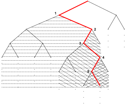
Figure 5.2. $\left\{\omega\right\}=\bigcap_{k=1}^{\infty}E\left(\omega|_{k}\right)$. Monotone families of tail sets. Let $\Omega_{N}$ be the set of all infinite words, i.e., the infinite Cartesian product. Start with a fixed infinite word $\omega$, so $\omega$ in $\Omega_{N}$ (highlighted in 5.2.) For every positive $k$, we truncate $\omega$, thus forming a finite word $\omega|_{k}$. Then the set $E\left(\omega|_{k}\right)$ is the set of all infinite words that begin with $\omega|_{k}$, but unrestricted after $k$. The intersection in $k$ of all these sets $E\left(\omega|_{k}\right)$ is then the singleton $\left\{\omega\right\}$.

The remaining case is, if none of the possible containment holds, i.e., $f$ not contained in $g$, and $g$ not contained in $f$. In this case, $E_{f}\cap E_{g}=\emptyset$, and so both sides in equation (4.40) are zero. See also Fig 5.2.

Having verified that $\mathbb{Q}_{\pi}$ satisfies condition (4.25) for basic cylinder-sets, it now follows that it must also hold for all pairs of sets $E,E^{\prime}\in\mathscr{C}$. This is an application of the Kolmogorov extension principle. The proof of the theorem is concluded. ∎

Corollary 4.15.

Let the setting be as above, $\pi\in Rep\left(\mathcal{O}_{N},\mathscr{H}\right)$, and let $\mathbb{Q}_{\pi}\left(\cdot\right)$ be the corresponding projection valued measure.

1. For $\omega\in\Omega_{N}$, and $k\in\mathbb{N}$, set $Z_{k}\left(\omega\right)=\omega_{k}\left(\in A_{N}\simeq\left\{1,2,\cdots,N\right\}\right)$, then the following projection-valued Markov property holds: Let $k>1$, then

   $$\text{$\mathbb{P}$rob}^{\left(\pi\right)}\left(Z_{k+1}=j\mid Z_{k}=i\right)=\beta_{\pi}^{k-1}\left(S_{i}S_{j}S_{j}^{*}S_{i}^{*}\right),$$ (4.41)

   where $\beta_{\pi}$ is the endomorphism in Definition 4.1 (eq. (4.2)).

2. If $\psi\in\mathscr{H}$, $\left\|\psi\right\|=1$, let $\mu_{\psi}\left(\cdot\right):=\left\langle\psi,\mathbb{Q}_{\pi}\left(\cdot\right)\psi\right\rangle_{\mathscr{H}}$ be the corresponding scalar valued measure. Then the associated transition probabilities are

   $$\text{$\mathbb{P}$rob}^{\left(\mu_{\psi}\right)}\left(Z_{k+1}=j\mid Z_{k}=i\right) =\frac{\left\langle\psi,\beta_{\pi}^{k-1}\left(S_{i}S_{j}S_{j}^{*}S_{i}^{*}\right)\psi\right\rangle_{\mathscr{H}}}{\left\langle\psi,\beta_{\pi}^{k-1}\left(S_{i}S_{i}^{*}\right)\psi\right\rangle_{\mathscr{H}}}$$

   $$=\frac{\left\|\beta_{\pi}^{k-1}\left(S_{j}^{*}S_{i}^{*}\right)\psi\right\|_{\mathscr{H}}^{2}}{\left\|\beta_{\pi}^{k-1}\left(S_{i}^{*}\right)\psi\right\|_{\mathscr{H}}^{2}}.$$ (4.42)

3. The Markov property holds for the process in (ii) if and only if $\beta_{\pi}$-invariance holds, in the following sense:

   $$\left\langle\psi,\beta_{\pi}\left(\mathbb{Q}_{\pi}\left(\cdot\right)\right)\psi\right\rangle_{\mathscr{H}}=\left\langle\psi,\mathbb{Q}_{\pi}\left(\cdot\right)\psi\right\rangle_{\mathscr{H}}=\mu_{\psi}\left(\cdot\right).$$

Proof.

For (4.41), we have

$$\text{$\mathbb{P}$rob}^{\left(\pi\right)}\left(Z_{k+1}=j\mid Z_{k}=i\right) =\sum_{I\in\mathbb{Z}_{N}^{k-1}}\mathbb{Q}_{\pi}\left(E\left(Iij\right)\right)$$

$$=\sum_{I\in\mathbb{Z}_{N}^{k-1}}S_{I}S_{i}S_{j}S_{j}^{*}S_{i}^{*}S_{I}^{*}\underset{\left({\scriptscriptstyle\text{by $\left(\ref{eq:e2}\right)$}}\right)}{=}\beta_{\pi}^{k-1}\left(S_{i}S_{j}S_{j}^{*}S_{i}^{*}\right).$$

Parts (ii) and (iii) follow immediately from this. ∎

Monic Representations.

Let $\pi\in Rep\left(\mathcal{O}_{N},\mathscr{H}\right)$, and let $\mathbb{Q}_{\pi}$ be the corresponding projection valued measure. Let $\mathfrak{M}_{\pi}$ be the abelian $*$-algebra generated by $\mathbb{Q}_{\pi}$, i.e., the operators

$$\int_{\Omega_{N}}f\left(\omega\right)\mathbb{Q}_{\pi}\left(d\omega\right)$$ (4.43)

where $f$ ranges over the measurable functions on $\left(\Omega_{N},\mathscr{C}\right)$.

Following [DJ14], we make the following:

Definition 4.16.

We say that $\pi$ is monic iff (Def.) there is a vector $\psi_{0}\in\mathscr{H}$, $\left\|\psi_{0}\right\|=1$, such that

$$\left[\mathfrak{M}_{\pi}\psi_{0}\right]=\mathscr{H},$$ (4.44)

i.e., $\psi_{0}$ is $\mathfrak{M}_{\pi}$-cyclic.

Starting with $\mathbb{Q}_{\pi}$ and (4.44), we use the construction outlined before Theorem 4.8, to get a scalar measure via:

$$\mu_{0}\left(E\right)=\left\langle\psi_{0},\mathbb{Q}_{\pi}\left(E\right)\psi_{0}\right\rangle_{\mathscr{H}},\;E\in\mathscr{C}.$$ (4.45)

Using [DJ14], we then get a random variable $Y:\Omega_{N}\rightarrow M$ for a measure space $\left(M,\mathscr{B}\right)$ such that the measure $\mu:=\mu_{0}\circ Y^{-1}$ satisfies the conditions listed below:

It was proved in [DJ14] that a representation $\pi\left(\in Rep\left(\mathcal{O}_{N},\mathscr{H}\right)\right)$ is monic iff it is unitarily equivalent to one realized in $L^{2}\left(M,\mu\right)$ as follows for some measure space $\left(M,\mu\right)$:

There are endomorphisms $\left(\left\{\tau_{i}\right\}_{i=1}^{N},\sigma\right)$, such that $\sigma\circ\tau_{i}=id_{M}$, $\mu\circ\tau_{i}^{-1}\ll\mu$, and $L^{2}\left(\mu\right)$-function $f_{i}$ on $M$, such that

$$\frac{d\left(\mu\circ\tau_{i}^{-1}\right)}{d\mu} =\left|f_{i}\right|^{2},\;1\leq i\leq N,$$ (4.46)

$$f_{i}\neq 0 \quad a.e.\;\mu\;\text{in }\tau_{i}\left(M\right).$$ (4.47)

Then the isometries $S_{i}$ are as follows:

$$S_{i}^{\left(\mu\right)}\varphi=f_{i}\left(\varphi\circ\sigma\right),\;1\leq i\leq N,$$ (4.48)

i.e., $\left\{S_{i}^{\left(\mu\right)}\right\}_{i=1}^{N}\in Rep\left(\mathcal{O}_{N},L^{2}\left(\mu\right)\right)$; see (3.6).

4.2. Atoms of the Path-Space Measure $\mathbb{Q}_{\pi}\left(\cdot\right)$

In Section 3 we introduced a random variable $X$ on path space $\left(\Omega_{N},\mathscr{C}\right)$; and in Section 4, a path-space-measure $\mathbb{Q}_{\pi}\left(\cdot\right)$. The starting point in both cases is a fixed $\pi\in Rep\left(\mathcal{O}_{N},\mathscr{H}\right)$. Specifically, a separable Hilbert space $\mathscr{H}$ is given, $N\in\mathbb{N}$, $N\geq 2$, fixed; and $\pi$ is a representation of $\mathcal{O}_{N}$, $\pi\in Rep\left(\mathcal{O}_{N},\mathscr{H}\right)$, $\pi\left(s_{i}\right)=:S_{i}$, $1\leq i\leq N$, with the isometries $S_{i}:\mathscr{H}\rightarrow\mathscr{H}$ satisfying (3.6). To summarize, the random variable $X=X_{\pi}$ is specified in (3.11) in Theorem 3.2, and the path-space measure $\mathbb{Q}_{\pi}$ in Theorem 4.8. Both take values in the projections in $\mathscr{H}$, see Section 2, and also [AJ15, AJL17, AJL18].

The question addressed here is: What are the atoms of $\mathbb{Q}_{\pi}$?

We say that a sample path $\omega\in\Omega_{N}$ is an atom if the singleton $\left\{\omega\right\}$ satisfies $\mathbb{Q}\left(\left\{\omega\right\}\right)>0$; so the closed subspace $\mathbb{Q}_{\pi}\left(\left\{\omega\right\}\right)\mathscr{H}=\mathscr{H}_{\omega}$ is non-zero. The answer to the question is given in the corollary below where we prove the following:

$$\mathbb{Q}_{\pi}\left(\left\{\omega\right\}\right)=X_{\pi}\left(\omega\right),\;\forall\omega\in\Omega_{N}.$$ (4.49)

We note that (4.49) holds even if one of the two sides (and hence both) is zero.

Details:

Corollary 4.17.

We have:

$$X_{\pi}\left(\omega\right)=\mathbb{Q}_{\pi}\left(\left\{\omega\right\}\right),\;\forall\omega\in\Omega_{N}.$$ (4.50)

Proof.

Fix $\omega\in\Omega_{N}$, then

$$\left\{\omega\right\}=\bigcap_{k=1}^{\infty}E\left(\omega|_{k}\right);$$ (4.51)

see also Fig 5.2. To see (4.51), note that

$$E\left(\omega|_{k}\right)=\left\{\xi\in\Omega_{N}\mid\xi_{i}=\omega_{i},\;1\leq i\leq k\right\},$$ (4.52)

so that $\xi\in\bigcap_{k}E\left(\omega|_{k}\right)\Longleftrightarrow\xi=\omega$ (see Fig 5.2). ∎

Remark 4.18.

The notation in (4.51) is consistent with convergence along a filter (see e.g. [Bou98, Wil04]) as follows: Let $\Omega_{N}=A^{\mathbb{N}}$ be as above where $A$ is a given (and fixed) alphabet. If $f=\left(x_{1},x_{2},\cdots,x_{k}\right)$, $x_{i}\in A$, is a finite path, we introduced the sets $E_{f}$ (or $E\left(f\right)$) where

$$E_{f}:=\left\{\omega\in\Omega_{N}\mid\omega_{i}=x_{i},\;1\leq i\leq k\right\}.$$ (4.53)

In particular, if $\omega\in\Omega_{N}$, $k\in\mathbb{N}$, set $f=\omega|_{k}=\left(\omega_{1},\omega_{2},\cdots,\omega_{k}\right)$ and we get the sets in (4.52).

Now consider the filter $\mathscr{F}$ of subsets of $\Omega_{N}$, defined as follows:

A subset $$E \mathscr{F} \big{[} \exists f E_{f}\subseteq E$$ is in iff (Def.) (a finite word) such that ]. (4.54)

(We say that $\left\{E_{f}\right\}$ forms a filter basis.)

The sets in $\mathscr{F}$ satisfy the two filter axioms:

1. If $E_{i}$, $i=1,2$, are in $\mathscr{F}$, then $\exists F\in\mathscr{F}$ such that $F\subseteq E_{i}$, for $i=1,2$.

2. If $E\in\mathscr{F}$, and $F$ is a subset of $\Omega_{N}$ such that $E\subseteq F$, then $F\in\mathscr{F}$.

Now condition (4.51) above is the assertion that

$$\lim_{k\>\mathscr{F}}\omega|_{k}=\omega;$$ (4.55)

stating that $E\left(\omega|_{k}\right)$, $k\in\mathbb{N}$, converges to $\left\{\omega\right\}$ along the filter $\mathscr{F}$.

4.3. Symbol Space Representations as Groups

In the study of iterated function systems (IFSs), and more generally, in symbolic dynamics, we consider a fixed finite alphabet $A$, as well as words in $A$. Both finite as well as infinite words are needed. For many purposes, it is helpful to give $A$ in the form of a cyclic group $\mathbb{Z}\big{/}N\mathbb{Z}\simeq\left\{0,1,2,\cdots,N-1\right\}$. In this case both the finite words $\Omega_{N}^{*}$, as well as infinite words $\Omega_{N}:=A^{\mathbb{N}}$ become groups. In the representation below, we identify $\Omega_{N}^{*}$, and $\Omega_{N}$, as a pair of abelian groups in duality. Since $\Omega_{N}^{*}$ (finite words) is discrete, we get $\Omega_{N}$ realized as a compact abelian group.

Lemma 4.19.

Let $N\in\mathbb{N}$, $N\geq 2$, be fixed, and let $\Omega_{N}^{*}$, resp. $\Omega_{N}$, denote the finite, resp., infinite words in $\mathbb{Z}_{N}\simeq\mathbb{Z}\big{/}N\mathbb{Z}$.

1. If $x=\left(x_{j}\right)_{j=1}^{\infty}\in\Omega_{N}$, and $y=\left(y_{j}\right)_{j=1}^{finite}\in\Omega_{N}^{*}$, are fixed, then set

   $$\left\langle x,y\right\rangle:=\prod_{k=1}^{\infty}\exp\left(i2\pi\left(\frac{x_{k}y_{k}}{N^{k}}\right)\right),$$ (4.56)

   so we have

   $$\left\langle x+x^{\prime},y\right\rangle =\left\langle x,y\right\rangle\left\langle x^{\prime},y\right\rangle,\;\text{and}$$ (4.57)

   $$\left\langle x,y+y^{\prime}\right\rangle =\left\langle x,y\right\rangle\left\langle x,y^{\prime}\right\rangle,$$ (4.58)

   for all $x,x^{\prime}\in\Omega_{N}$, and $y,y^{\prime}\in\Omega_{N}^{*}$.

2. In the category of abelian groups, we get

   $$dual\left(\Omega_{N}\right) =\Omega_{N}^{*},$$ and (4.59)

   $$dual\left(\Omega_{N}^{*}\right) =\Omega_{N},$$ where (4.60)

   “dual” refers to Pontryagin duality. Note $\Omega_{N}^{*}=\bigcup_{k=1}^{\infty}N^{-k}\mathbb{Z}$; and

   $$\mathbb{Z}\subset N^{-1}\mathbb{Z}\subset N^{-2}\mathbb{Z}\subset\cdots\subset N^{-k}\mathbb{Z}\subset N^{-\left(k+1\right)}\mathbb{Z}\subset\cdots.$$ (4.61)

3. The Haar measure on $\Omega_{N}$ is the infinite product norm on $\left(\mathbb{Z}_{N}\right)^{\mathbb{N}}$ with weights $\left(\frac{1}{N},\frac{1}{N},\cdots,\frac{1}{N}\right)$ on each factor.

Proof.

The lemma follows from results in the literature (see [DHJ15, DJ15]), and is left to the reader.

Identify a finite word $y=\left(y_{1},\cdots,y_{k}\right)\in\Omega_{N}^{*}$ ($y_{j}\in\mathbb{Z}_{N}=\left\{0,1,\cdots,N-1\right\}$) with

$$\tilde{y} =\frac{y_{1}N^{k-1}+\cdots+y_{k-1}N+y_{k}}{N^{k}}$$ (4.62)

$$=y_{1}/N+\cdots+y_{k}/N^{k}\in N^{-k}\mathbb{Z};$$

see (4.61). Set

$$S_{y}=S_{y_{1}}S_{y_{2}}\cdots S_{y_{k}};$$ (4.63)

and if $x=\left(x_{j}\right)_{j=1}^{\infty}\in\Omega_{N}$ ($x_{j}\in\mathbb{Z}_{N}$), define an automorphism action $\alpha\left(x\right)$ of $\mathcal{O}_{N}$ by its values on generators $S_{y}$ as follows:

$$\alpha\left(x\right)S_{y}=\left\langle x,y\right\rangle S_{y};$$ (4.64)

called the gauge-action.

In particular,

$$\alpha\left(x\right)\left(S_{y}S_{y}^{*}\right)=S_{y}S_{y}^{*}.$$ (4.65)

The abelian $*$-subalgebra $\mathfrak{M}_{N}$ in $\mathcal{O}_{N}$ generated by the projections $\left\{S_{y}S_{y}^{*}\right\}_{y\in\Omega_{N}^{*}}$ ($\Omega_{N}^{*}=$ finite words) is $\mathfrak{M}_{N}=\left\{M\in\mathcal{O}_{N}\mid\alpha\left(x\right)M=M,\;\forall x\in\Omega_{N}\right\}$. ∎

Remark 4.20.

It follows from Lemma 4.19 that the projection valued measures from Theorems 3.2 and 4.8 may be realized on the compact group $\Omega_{N}$.

For the study of Markov chains, the following extension of the lemma will be useful:

Lemma 4.21.

Let $M$ be a fixed $N\times N$ matrix over $\mathbb{Z}$, and assume its eigenvalues $\lambda_{j}$ satisfy $\left|\lambda_{j}\right|>1$.

From the nested chain of groups we then obtain inductive, and projective limits, in the form of discrete groups $\Omega_{M}^{*}$, and compact dual $\Omega_{M}$.

Case 1 (inductive)

$$\mathbb{Z}^{N}\big{/}M^{k+1}\mathbb{Z}^{N}\hookrightarrow\mathbb{Z}^{N}\big{/}M^{k}\mathbb{Z}^{N}$$ (4.66)

and the dual projective group formed from the groups

$$\left(M^{T}\right)^{k}\mathbb{Z}^{N}$$ (4.67)

where $M^{T}$ denotes the transposed matrix:

$$\Omega_{M}^{*}=\bigcup_{k=1}^{\infty}M^{-k}\left(\mathbb{Z}_{N}\right);$$

and note $\mathbb{Z}_{N}\subset M^{-1}\mathbb{Z}_{N}\subset M^{-2}\mathbb{Z}_{N}\subset\cdots\subset M^{-k}\mathbb{Z}_{N}\subset M^{-\left(k+1\right)}\mathbb{Z}_{N}\subset\cdots$.

When $M$ is fixed, and pair $x=\left(x_{j}\right)$ and $y=\left(y_{j}\right)$ are infinite, resp., finite, words in $\mathbb{Z}^{N}\big{/}M\mathbb{Z}^{N}$, then the Pontryagin duality is then

$$\left\langle x,y\right\rangle_{M}:=\prod_{k=1}^{\infty}\exp\left(i2\pi\left(M^{T}\right)^{-k}x_{j}\cdot y_{j}\right).$$ (4.68)

Proof.

See, e.g., [BJKR01, BJKR02, BJOk04].

Note that if $x$ and $y$ $\in\mathbb{Z}^{N}$, and $k\in\mathbb{N}$, then in the quotient group we have

$$\left(M^{T}\right)^{-k}x\cdot y=\left(M^{T}\right)^{-\left(k+1\right)}x\cdot My.$$

∎

5. Iterated Function Systems (IFS), and $Rep\left(\mathcal{O}_{N},\mathscr{H}\right)$

Recall, when $N$ is a fixed integer, at least 2, the corresponding Cuntz algebra $\mathcal{O}_{N}$ has a rich family of representations (see, e.g., [Gli60, Gli61, Cun77, BJ02, BJOk04]). They are studied in the previous two sections, with the use of the associated projection-valued measures. As noted in Section 4.3, some of the $\mathcal{O}_{N}$ representations correspond to iterated function systems (IFSs), where the iteration of branching laws is given by a system of $N$ prescribed endomorphisms in a measure space. One reason the use of IFSs is powerful is that the framework allows one to make precise iteration of self-similarity in Cantor-dynamics, and, more generally, in non-reversible dynamics, as well as the corresponding “chaos-limits.” (See [Hut81, Hut95, DJ14, AJL17].) The setting of IFS-systems includes a rich class of fractals, e.g., those corresponding to affine IFSs, and others to complex dynamics.

Two themes are addressed in this section: (i) We present the correspondence between representations of the Cuntz algebra $\mathcal{O}_{N}$, on one hand, and IFSs with $N$ generating endomorphisms, on the other. (ii) Our focus will be a use of the $\mathcal{O}_{N}$ representations in a realization of generalized Martin boundaries for the IFSs under consideration. For this purpose, it will be convenient to first fix an alphabet $A$, of size $N$. We then consider kernels indexed by both finite words in $A$, as well as by infinite words; see Section 4 for details.

In Theorem 5.8 below, we show that such a boundary theory may be derived from the random variables $Y$ which we introduced in Section 3. In broad outline, our boundary representations will be obtained as limits of kernels indexed initially by finite words in the alphabet A; – the limit referring to finite vs infinite words in the symbolic representations. This theme will be expanded further in Section 7 below.

The present section concludes with a number of explicit examples.

Let $\left(M,d\right)$ be a compact metric space, $N\in\mathbb{N}$ fixed, $N\geq 2$,

$$p_{1},\cdots,p_{N},\;,p_{i}>0,\;\sum_{i=1}^{N}p_{i}=1,\text{ fixed.}$$ (5.1)

Let $\tau_{i}:M\rightarrow M$, $1\leq i\leq N$, be a system of strict contractions in $\left(M,d\right)$. Let $\Omega_{N}=\left\{1,2,\cdots,N\right\}^{\mathbb{N}}$, and let

$$\mathbb{P}=\vartimes{}_{1}^{\infty}p=\underset{\aleph_{0}\text{ product measure}}{\underbrace{p\times p\times p\cdots\cdots}}$$ (5.2)

(see [Kak43, Hid80].)

In this section, we construct random variables $Y$ with values in $M$ (some measure space $\left(M,\mathscr{B}_{M}\right)$), so $Y:\Omega\rightarrow M$, such that the corresponding distribution $\mu:=\mathbb{P}\circ Y^{-1}$ satisfies

$$\mu=\sum_{i=1}^{N}p_{i}\mu\circ\tau_{i}^{-1}.$$

Here $\mathbb{P}$ is the infinite -product measure (5.2).

Example 5.1 (A Julia construction).

Although the early analysis (e.g., [Hut81]) of many of the iterated function systems (IFSs) focused on iteration of systems of affine maps in some ambient $\mathbb{R}^{d}$, there is also a rich literature dealing with complex dynamics, and iteration of conformal maps, see e.g., [Mil06]. Also in these cases, there are IFS measures, see Theorem 5.2 ii. In the simplest cases these Julia iteration limits arise from an iteration of branches of the inverse of complex polynomials. The corresponding IFS limits are typically Julia sets; named after Gaston Julia. Examples are included in Fig 5.1.

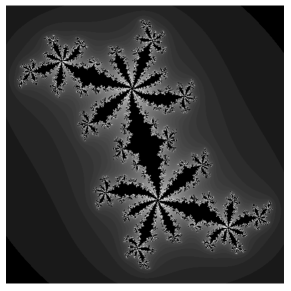
(a) $c=0.125+0.625i$

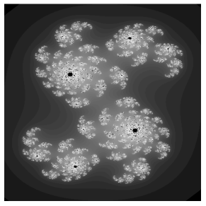
(b) $c=0.375-0.125i$

Figure 5.1. $\mathbb{C}\ni z\rightarrow z^{2}+c$ ($c\in\mathbb{C}\backslash\left\{0\right\}$ fixed), $\tau_{\pm}:z\rightarrow\pm\sqrt{z-c}$.

Theorem 5.2.

For points $\omega=\left(i_{1},i_{2},i_{3},\cdots\right)\in\Omega_{N}$ and $k\in\mathbb{N}$, set

$$\omega\big{|}_{k} =\left(i_{1},i_{2},\cdots,i_{k}\right),\;\text{and}$$ (5.3)

$$\tau_{\omega|_{k}} =\tau_{i_{1}}\circ\tau_{i_{2}}\circ\cdots\circ\tau_{i_{k}}.$$ (5.4)

Then $\bigcap_{k=1}^{\infty}\tau_{\omega|_{k}}$$\left(M\right)$ is a singleton, say $\left\{x\left(\omega\right)\right\}$. Set $Y\left(\omega\right)=x\left(\omega\right)$, i.e.,

$$\left\{Y\left(\omega\right)\right\}=\bigcap_{k=1}^{\infty}\tau_{\omega|_{k}}\left(M\right);$$ (5.5)

then:

1. $Y:\Omega_{N}\rightarrow M$ is an $\left(M,d\right)$-valued random variable.

2. The distribution of $Y$, i.e., the measure

   $$\mu=\mathbb{P}\circ Y^{-1}$$ (5.6)

   is the unique Borel probability measure on $\left(M,d\right)$ satisfying:

   $$\mu=\sum_{i=1}^{N}p_{i}\mu\circ\tau_{i}^{-1};$$ (5.7)

   equivalently,

   $$\int_{M}fd\mu=\sum_{i=1}^{N}p_{i}\int_{M}\left(f\circ\tau_{i}\right)d\mu,$$ (5.8)

   holds for all Borel functions $f$ on $M$.

3. The support $M_{\mu}=supp\left(\mu\right)$ is the minimal closed set (IFS), $\neq\emptyset$, satisfying

   $$M_{\mu}=\bigcup_{i=1}^{\infty}\tau_{i}\left(M_{\mu}\right).$$ (5.9)

$$E\left(\omega|_{1}\right)\supset E\left(\omega|_{2}\right)\supset\cdots\supset E\left(\omega|_{k}\right)\supset E\left(\omega|_{k+1}\right)\supset\cdots$$

Proof.

We shall make use of standard facts from the theory of iterated function systems (IFS), and their measures; see e.g., [Hut81, BHS08, Hut95].

Proof of (5.5). We use that when $\omega\in\Omega_{N}$ is fixed then the sets $\tau_{\omega|_{k}}\left(M\right)$ is a monotone family of compact subsets

$$\tau_{\omega|_{k+1}}\left(M\right)\subset\tau_{\omega|_{k}}\left(M\right),$$ (5.10)

and since $\tau_{i}$ is strictly contractive for all $i$, we get

$$\lim_{k\rightarrow\infty}diameter\left(\tau_{\omega|_{k}}\left(M\right)\right)=0,$$ (5.11)

and so (5.5) follows; i.e., the intersection $\bigcap_{i=1}^{\infty}$ is a singleton depending only on $\omega$.

Monotonicity: This conclusion again follows from the assumptions placed on $\left\{\tau_{i}\right\}_{i=1}^{N}$, but we shall specify the respective $\sigma$-algebras, the one on $\Omega_{N}$ and the one on $M$.

The $\sigma$-algebra of subsets of $\Omega_{N}$ will be generated by cylinder sets: If $f=\left(i_{1},i_{2},\cdots,i_{k}\right)$ is a finite word, the corresponding cylinder set $E\left(f\right)\subset\Omega_{N}$ is

$$E\left(f\right)=\left\{\omega\in\Omega_{N}\mid\omega_{j}=i_{j},\;1\leq j\leq k\right\}.$$ (5.12)

On $M$, we pick the Borel $\sigma$-algebra determined from the fixed metric $d$ on $M$. The measure $\mathbb{P}=\mathbb{P}_{p}$ is specified by its values on cylinder sets; i.e, set

$$\mathbb{P}\left(E\left(f\right)\right)=p_{i_{1}}p_{i_{2}}\cdots p_{i_{k}}=:p_{f}$$ (5.13)

where the numbers $p_{1},\cdots,p_{N}$ are as in (5.1).

Proof of (5.7). The argument is based on the following: On $\Omega_{N}$, introduce the shifts $\hat{\tau}_{b}\left(i_{1},i_{2},i_{3},\cdots\right)=\left(b,i_{1},i_{2},i_{3},\cdots\right)$, $b\in\left\{1,2,\cdots,N\right\}$, and let $Y$ be as in (5.5)-(5.6). Then

$$\tau_{b}Y=Y\hat{\tau}_{b},$$ (5.14)

or equivalently,

$$\tau_{b}\left(Y\left(\omega\right)\right)=Y\left(\hat{\tau}_{b}\left(\omega\right)\right),\;\forall\omega\in\Omega_{N}.$$ (5.15)

Now (5.15) is immediate from (5.5).

We now show (5.8), equivalently (5.7). Let $f$ be a Borel function on $M$, then

$$\int_{M}f\,d\mu =\int_{\Omega_{N}}\left(f\circ Y\right)d\mathbb{P} \left(\text{by }\left(\ref{eq:d6}\right)\right)$$

$$=\sum_{i=1}^{N}p_{i}\int_{\Omega_{N}}f\circ Y\circ\hat{\tau}_{i}\>d\mathbb{P} \left(\begin{matrix}\text{since $\mathbb{P}$ is the product}\\ \text{ measure $\vartimes_{1}^{\infty}p$, see $\left(\ref{eq:d13}\right)$}\end{matrix}\right)$$

$$=\sum_{i=1}^{N}p_{i}\int_{\Omega_{N}}f\circ\tau_{i}\circ Y\>d\mathbb{P} \left(\text{by }\left(\ref{eq:d14}\right)\right)$$

$$=\sum_{i=1}^{N}p_{i}\int_{M}f\circ\tau_{i}\>d\mu \left(\text{by }\left(\ref{eq:d6}\right)\right)$$

which is the desired conclusion. ∎

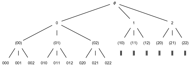
Figure 5.3. Encoding of words into IFS. Infinite words $\omega\in\Omega$ $\longrightarrow$ singletons in the Sierpinski gasket.

Using $\Omega_{N}=\left\{1,2,\cdots,N\right\}^{\mathbb{N}}$ for encoding iterated function systems (IFS).

Example 5.3 (Sierpinski gasket).

$M=\left[0,1\right]\times\left[0,1\right]$ with the usual metric,

$$\tau_{0}\left(x,y\right)=\left(\frac{x}{2},\frac{y}{2}\right),\quad\tau_{1}\left(x,y\right)=\left(\frac{x+1}{2},\frac{y}{2}\right),\quad\tau_{2}\left(x,y\right)=\left(\frac{x}{2},\frac{y+1}{2}\right),$$

and so the Sierpinski gasket $M_{Si}$ satisfies

$$M_{Si}=\tau_{0}\left(M_{Si}\right)\bigcup\tau_{1}\left(M_{Si}\right)\bigcup\tau_{2}\left(M_{Si}\right).$$

See Figure 5.3.

5.1. The Projection Valued Path Space Measure Corresponding to IFS Representations

In Theorem 5.2, we introduced the class of contractive iterated function systems (IFSs), $\left\{\tau_{i}\right\}_{i=1}^{N}$. We shall point out that, for each of these IFSs, there is a natural representation of $\mathcal{O}_{N}$; as follows:

For simplicity, we shall assume in addition to the conditions listed in Theorem 5.2, that we also have non-overlap as follows: If $i\neq j$, then we assume

$$\mu\left(\tau_{i}\left(M\right)\cap\tau_{j}\left(M\right)\right)=0.$$ (5.16)

We also fix weights $\left\{p_{i}\right\}_{i=1}^{N}$, and we let $\mu$ be the corresponding IFS-measure, see (5.7) in the theorem. Also we recall the associated endomorphism $\sigma$ in $\left(M,d\right)$ satisfying:

$$\sigma\circ\tau_{i}=id_{M},\;\forall i=1,\cdots,N.$$ (5.17)

Once (5.16) is assumed, it is easy to construct $\sigma$ such that (5.17) holds, i.e., the system $\left\{\tau_{i}\right\}_{i=1}^{N}$ constitutes branches of the inverse for $\sigma$, and

$$\sigma^{-1}\left(E\right)=\bigcup_{i=1}^{N}\tau_{i}\left(E\right)$$ (5.18)

for all Borel subsets $E\subset M$.

Proposition 5.4.

Let $\left(\left\{\tau_{i}\right\}_{i=1}^{N},\left\{p_{i}\right\}_{i=1}^{N},\mu\right)$ be as stated; and set $\mathscr{H}=L^{2}\left(M,\mu\right)$. Then the following operators $\left\{S_{i}\right\}_{i=1}^{N}$, $\left\{S_{i}^{*}\right\}_{i=1}^{N}$ constitute a representation

$$\pi\in Rep\left(\mathcal{O}_{N},L^{2}\left(\mu\right)\right).$$ (5.19)

We set, for $f\in L^{2}\left(\mu\right)$:

$$S_{i}f=\frac{1}{\sqrt{p_{i}}}\chi_{\tau_{i}\left(M\right)}f\circ\sigma$$ (5.20)

and

$$S_{i}^{*}f=\sqrt{p_{i}}f\circ\tau_{i}.$$ (5.21)

Proof.

Let $S_{i}$, $S_{i}^{*}$ denote the system of $2N$ operators in $L^{2}\left(\mu\right)$, given in (5.20)-(5.21). It is immediate that $S_{i}^{*}S_{j}=\delta_{ij}I_{L^{2}\left(\mu\right)}$. For this we use that

$$\chi_{\tau_{i}\left(M\right)}\circ\tau_{j}=\delta_{ij}\mathbbm{1},$$ (5.22)

the constant function $\mathbbm{1}$ in $L^{2}\left(\mu\right)$.

A direct computation using (5.7) in Theorem 5.2 yields

$$\int_{M}f\,\left(S_{i}g\right)d\mu=\int_{M}\left(S_{i}^{*}f\right)g\,d\mu,$$ (5.23)

valid for all $f,g\in L^{2}\left(\mu\right)$.

Moreover, we have

$$S_{i}S_{i}^{*}=\text{multiplication by $\chi_{\tau_{i}\left(M\right)}$ in $L^{2}\left(M\right)$. }$$ (5.24)

Since $\bigcup_{i=1}^{N}\tau_{i}\left(M\right)=M$, as a disjoint union, we also get

$$\sum_{i=1}^{N}S_{i}S_{i}^{*}=I_{L^{2}\left(\mu\right)},$$ (5.25)

and so $\pi\in Rep\left(\mathcal{O}_{N},L^{2}\left(\mu\right)\right)$ as asserted in the Proposition. ∎

Corollary 5.5.

Let $\left\{\tau_{i}\right\}_{i=1}^{N}$ and $\pi\in Rep\left(\mathcal{O}_{N},L^{2}\left(\mu\right)\right)$ be as in Proposition 5.4; then for the projection-valued path space measure $\mathbb{Q}_{\pi}$ in Theorem 4.8, we have the following formula:

Let $f=\left(i_{1},\cdots,i_{N}\right)$ be a finite word, and let $E_{f}$ denote the corresponding basic cylinder subset, $E_{f}\subseteq\Omega_{N}$, then

$$\mathbb{Q}_{\pi}\left(E_{f}\right) =\text{multiplication by the indicator }$$

$$\quad\quad\text{function $\chi_{\tau_{i_{1}}\tau_{i_{2}}\cdots\tau_{i_{k}}\left(M\right)}$}.$$ (5.26)

Proof.

Immediate from Theorem 4.8. ∎

A self-dual representation.

Corollary 5.6.

Let the setting be as in Proposition 5.4 and Corollary 5.5. In particular, we fix $\big{(}N,\left\{p_{i}\right\}_{i=1}^{N},\mu\big{)}$, and the $\mathcal{O}_{N}$-representation $\pi^{\left(\mu\right)}:=\big{\{}S_{i}^{\left(\mu\right)}\big{\}}_{i=1}^{N}$ as specified in (5.20)-(5.21). This representation is self-dual in the following sense.

Let $\mathbbm{1}$ denote the constant function $\mathbbm{1}$ in $L^{2}\left(M,\mu\right)$, and let $\mathbb{Q}_{\pi}$ be the corresponding projection valued measure (see Corollary 4.14). Set

$$\left\langle\mathbbm{1},\mathbb{Q}_{\pi}\left(\cdot\right)\mathbbm{1}\right\rangle_{L^{2}\left(\mu\right)}=\nu_{\pi}\left(\cdot\right),$$ (5.27)

as a measure on $\Omega_{N}$; then

$$\nu_{\pi}\circ Y^{-1}=\mu.$$ (5.28)

Proof.

Since $\pi^{\left(\mu\right)}=\big{\{}S_{i}^{\left(\mu\right)}\big{\}}_{i=1}^{N}$ in (5.20)-(5.21) is in $Rep\left(\mathcal{O}_{N},L^{2}\left(\mu\right)\right)$, we get from (5.25):

$$\sum_{i=1}^{N}\left\|S_{i}^{\left(\mu\right)*}f\right\|_{L^{2}\left(\mu\right)}^{2}=\left\|f\right\|_{L^{2}\left(\mu\right)}^{2},\;\forall f\in L^{2}\left(\mu\right).$$ (5.29)

Introducing (5.21), we then conclude:

$$\sum_{i=1}^{N}p_{i}\int_{M}\left|f\right|^{2}\circ\tau_{i}\,d\mu=\int_{M}\left|f\right|^{2}d\mu,$$

and so, by (5.24),

$$\int_{M}\left|f\right|^{2}d\mu=\int_{\Omega_{N}}\left(\left|f\right|^{2}\circ Y\right)d\nu_{\pi}=\int_{M}\left|f\right|^{2}d\left(\nu_{\pi}\circ Y^{-1}\right),$$

valid for all $f\in L^{2}\left(\mu\right)$. The desired conclusion (5.28) follows. ∎

5.2. Boundaries of Representations

Let $M$ be a compact Hausdorff space, with Borel $\sigma$-algebra $\mathscr{B}$, and let $A$ be a finite alphabet, $\left|A\right|=N$. Let $\left\{\tau_{i}\right\}_{i\in A}$ be a system of endomorphisms. For every $\omega\in\Omega_{N}\left(=A^{\mathbb{N}}\right)$, and $k\in\mathbb{N}$, set $\omega|_{k}=\left(\omega_{1},\cdots,\omega_{k}\right)$ (= the truncated finite word), and set

$$\tau_{\omega|_{k}}=\tau_{\omega_{1}}\circ\cdots\circ\tau_{\omega_{k}}.$$ (5.30)

Definition 5.7.

We say that $\left\{\tau_{i}\right\}_{i\in A}$ is tight iff

$$\bigcap_{k=1}^{\infty}\tau_{\omega|_{k}}\left(M\right)=\left\{Y\left(\omega\right)\right\}$$ (5.31)

is a singleton for $\forall\omega\in\Omega_{N}$; and we define $Y:\Omega_{N}\rightarrow M$ by eq. (5.31).

Theorem 5.8.

Let $\left(M,\left\{\tau_{i}\right\}_{i\in A}\right)$ be as above, assume tight. Let $\pi\in Rep\left(\mathcal{O}_{N},\mathscr{H}\right)$ for some Hilbert space, and let $\mathbb{Q}_{\pi}$ be the corresponding projection-valued measure. Assume $\mathbb{Q}_{\pi}$ has one-dimensional range; see Corollary 4.14; set

$$\mu:=\mathbb{Q}_{\pi}\circ Y^{-1}.$$ (5.32)

Then for all $\omega\in\Omega_{N}=A^{\mathbb{N}}$, we have

$$\mu\circ\tau_{\omega|_{k}}^{-1}\xrightarrow[\;k\rightarrow\infty\;]{}\delta_{Y\left(\omega\right)},$$ (5.33)

i.e., for all $f\in C\left(M\right)$, we have

$$\lim_{k\rightarrow\infty}\int_{M}f\circ\tau_{\omega|_{k}}d\mu=f\left(Y\left(\omega\right)\right).$$ (5.34)

Proof.

Let $\varepsilon>0$. Since $f$ is uniformly continuous, there is a neighborhood $O_{\omega}$ of $Y\left(\omega\right)$ such that

$$\left|f\left(y\right)-f\left(y^{\prime}\right)\right|<\varepsilon\quad\text{for}\;\forall y,y^{\prime}\in O_{\omega}.$$ (5.35)

Since by assumption $\mu\left(M\right)=1$, we conclude from (5.35) and (5.31), that for $\forall k,l\geq k_{0}$, we have

$$\left|f\circ\tau_{\omega|_{k}}-f\circ\tau_{\omega|_{l}}\right|\leq\varepsilon;$$ (5.36)

as a uniform estimate on $M$. Since

$$\int_{M}f\circ\tau_{\omega|_{k}}d\mu=\int_{M}f\,d\left(\mu\circ\tau_{\omega|_{k}}^{-1}\right),$$ (5.37)

a second application of (5.31) now yields:

$$\lim_{k\rightarrow\infty}\int_{M}f\circ\tau_{\omega|_{k}}d\mu=f\left(Y\left(\omega\right)\right)$$

which is the desired conclusion. ∎

5.3. Three Examples

Below we give three examples of IFS-measures, as in Theorem 5.2: (i) the Lebesgue measure restricted to the unit interval $\left[0,1\right]$, (ii) the middle-third Cantor measure $\mu_{3}$, and (iii) the $\nicefrac{{1}}{{4}}$-Cantor measure $\mu_{4}$ with two gaps. Their respective properties follow from Theorem 5.2, and are summarized in Table 5.1. Also see Figures 5.4, 5.5, and 5.7.

The difference in the graphs of the cumulative distributions in Ex 2 and Ex 3, is explained by the following: In Ex 3, we have two omitted intervals in each iteration step, as opposed to just one in Ex 2, the Middle-third Cantor construction. See Fig 5.6.

$\left\{\tau_{i}\right\}_{i=1}^{2}$	$\sigma$	$\left(p_{i}\right)_{i=1}^{2}$	Scaling dimension (SD) of the IFS-measure $\left(\mu,M_{\mu}\right)$
$\tau_{0}\left(x\right)=\frac{x}{2}$, $\tau_{1}\left(x\right)=\frac{x+1}{2}$	$\sigma\left(x\right)=2x$ mod 1	$\left(\frac{1}{2},\frac{1}{2}\right)$	$\mu=\lambda=$ Lebesgue measure, SD = 1
$\tau_{0}\left(x\right)=\frac{x}{3}$, $\tau_{1}\left(x\right)=\frac{x+2}{3}$	$\sigma\left(x\right)=3x$ mod 1	$\left(\frac{1}{2},\frac{1}{2}\right)$	$\mu=\mu_{3}=$ middle-third Cantor measure, SD = $\frac{\ln 2}{\ln 3}$
$\tau_{0}\left(x\right)=\frac{x}{4}$, $\tau_{1}\left(x\right)=\frac{x+2}{4}$	$\sigma\left(x\right)=4x$ mod 1	$\left(\frac{1}{2},\frac{1}{2}\right)$	$\mu=\mu_{4}=$ the $\nicefrac{{1}}{{4}}$-Cantor measure, SD = $\frac{1}{2}$

Table 5.1. Three inequivalent examples, each with $\Omega_{N}=A^{\mathbb{N}}$, $\left|A\right|=2$, and infinite product measure $\vartimes_{1}^{\infty}\left(\frac{1}{2},\frac{1}{2}\right)$. See also Fig 5.7.

(a) The middle-third Cantor set.

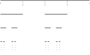
(b) The $\nicefrac{{1}}{{4}}$-Cantor set.

Figure 5.4. Examples of Cantor sets.

In each of the three examples in Table 5.1, we give the initial step in the IFS iteration. Each IFS-limit yields a measure, and a support set. The second and the third examples are the fractal limits known as the Cantor measure $\mu_{3}$, and the Cantor measure $\mu_{4}$. The details of the iteration steps are outlined in the subsequent figures and algorithms. Figures 5.5 and 5.6 deal with the associated cumulative distribution $F\left(x\right):=\mu\left(\left[0,x\right]\right)$. The latter will be used in Section 7.3 at the end of our paper.

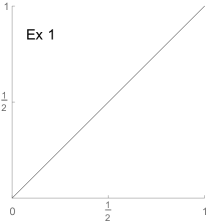
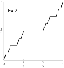
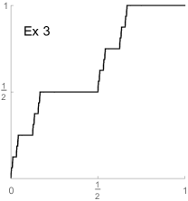
$F_{\lambda}\left(x\right)=\lambda\left(\left[0,x\right]\right)$; points of increase = the support of the normalized $\lambda$, so the interval $[0,1]$.	$F_{\nicefrac{{1}}{{3}}}\left(x\right)=\mu_{3}\left(\left[0,x\right]\right)$; points of increase = the support of $\mu_{3}$, so the middle third Cantor set $C_{\nicefrac{{1}}{{3}}}$ (the Devil’s staircase).	$F_{\nicefrac{{1}}{{4}}}\left(x\right)=\mu_{4}\left(\left[0,x\right]\right)$; points of increase = the support of $\mu_{4}$, so the double-gap Cantor set $C_{\nicefrac{{1}}{{4}}}$.

Figure 5.5. The three cumulative distributions. The three support sets, $[0,1]$, $C_{\nicefrac{{1}}{{3}}}$, and $C_{\nicefrac{{1}}{{4}}}$ are IFSs, and they are also presented in detail inside Table 5.1 above.

Figure 5.6. Illustration of $F_{\nicefrac{{1}}{{4}}}\left(x\right)=\mu_{4}\left(\left[0,x\right]\right)$ in Ex 3. Note that $\inf\{F_{\nicefrac{{1}}{{4}}}^{-1}\left(1/2\right)\}=\frac{1}{4}-\left(\sum_{n=2}^{\infty}\frac{1}{4^{n}}\right)=\frac{1}{6}$, and $\inf\{F_{\nicefrac{{1}}{{4}}}^{-1}\left(1\right)\}=\frac{2}{3}$.

Ex 1
	$\tau_{0}\left(x\right)=\frac{x}{2}$	$\tau_{1}\left(x\right)=\frac{x+1}{2}$	$\sigma\left(x\right)=2x$ mod 1
Ex 2
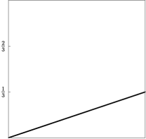
	$\tau_{0}\left(x\right)=\frac{x}{3}$	$\tau_{1}\left(x\right)=\frac{x+2}{3}$	$\sigma\left(x\right)=3x$ mod 1
Ex 3
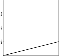
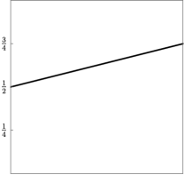
	$\tau_{0}\left(x\right)=\frac{x}{4}$	$\tau_{1}\left(x\right)=\frac{x+2}{4}$	$\sigma\left(x\right)=4x$ mod 1

Figure 5.7. The endomorphisms in the three examples.

Bit-representation of the respective IFSs in each of the three examples.

In the three examples from Table 5.1, the associated random variable $Y$ (from Theorem 5.2, eq (5.5)) is as follows:

Ex 1 $$Y_{\lambda}\left(\varepsilon_{i}\right)=\frac{1}{2}\sum_{i=1}^{\infty}\frac{\varepsilon_{i}}{2^{i}},$$

Ex 2 $$Y_{\mu_{3}}\left(\varepsilon_{i}\right)=\sum_{i=1}^{\infty}\frac{\varepsilon_{i}}{3^{i}},\quad\text{and}$$

Ex 3 $$Y_{\mu_{4}}\left(\varepsilon_{i}\right)=\sum_{i=1}^{\infty}\frac{\varepsilon_{i}}{4^{i}},\quad\varepsilon_{i}\in\left\{0,2\right\},\;\left(\varepsilon_{i}\right)\in\Omega_{2}.$$

Boundary Representation for the two measures $\mu_{3}$ and $\mu_{4}$, (see Theorem 5.2, and Figs 5.4-5.5.)

Definition 5.9.

Let $\mu$ be a (singular) measure with support contained in the interval $I=\left[0,1\right]\simeq\partial\mathbb{D}$, the boundary of the disk $\mathbb{D}=\left\{z\in\mathbb{Z}\mathrel{{;}}\left|z\right|<1\right\}$.

A function $K:\mathbb{D}\times I\rightarrow\mathbb{C}$ is said to be a boundary representation iff (Def) the following four axioms hold:

1. $K\left(\cdot,x\right)$ is analytic in $\mathbb{D}$ for all $x\in I$;

2. $K\left(z,\cdot\right)\in L^{2}\left(\mu\right)$, $\forall z\in\mathbb{D}$;

3. Setting, for $f\in L^{2}\left(I,\mu\right)$,

   $$\left(Kf\right)\left(z\right)=\int_{0}^{1}f\left(x\right)K\left(z,x\right)d\mu\left(x\right),$$ (5.38)

   then $Kf\in H_{2}\left(\mathbb{D}\right)$, the Hardy-space; and

4. The following limit exists in the $L^{2}\left(\mu\right)$-norm:

   $$\lim_{\begin{subarray}{c}r\nearrow 1\\ r<1\end{subarray}}\left(Kf\right)\left(r\,e\left(x\right)\right)=f\left(x\right),$$

   where $e\left(x\right):=e^{i2\pi x}$, $x\in I$.

We say that $K$ is self-reproducing if there is a kernel $K^{\mathbb{C}}:\mathbb{D}\times\mathbb{D}\rightarrow\mathbb{C}$ satisfying

$$\lim_{r\nearrow 1}K^{\mathbb{C}}\left(z,r\,e\left(x\right)\right)=K\left(z,x\right),\;\forall z\in\mathbb{D},\>x\in I;$$ (5.39)

and

$$\int_{0}^{1}K\left(z,x\right)\overline{K\left(w,x\right)}d\mu\left(x\right)=K^{\mathbb{C}}\left(z,w\right),\;\forall\left(z,w\right)\in\mathbb{D}\times\mathbb{D}.$$ (5.40)

Remark 5.10.

When $\left(K,K^{\mathbb{C}}\right)$ satisfy the two conditions (5.39)-(5.40), it is immediate that $K^{\mathbb{C}}$ is then a positive definite kernel on $\mathbb{D}\times\mathbb{D}$. We shall denote the corresponding reproducing kernel Hilbert space RKHS by $\mathscr{H}\left(K^{\mathbb{C}}\right)$; see [Aro50, AS57].

Furthermore, the assignment

$$T_{\mu}:\underset{{\scriptstyle\text{as a function on $\mathbb{D}$}}}{\underbrace{K^{\mathbb{C}}\left(\cdot,z\right)}}\longmapsto\underset{{\scriptstyle\text{in $L^{2}\left(I,\mu\right)$}}}{\underbrace{K\left(z,\cdot\right)}}$$ (5.41)

extends by linearity, and norm-closure to an isometry:

$$T_{\mu}:\mathscr{H}\left(K^{\mathbb{C}}\right)\longrightarrow L^{2}\left(\mu\right);$$ (5.42)

with “isometry” relative to the respective Hilbert norms in (5.42).

Moreover, the adjoint operator

$$T_{\mu}^{*}:L^{2}\left(\mu\right)\longrightarrow\mathscr{H}\left(K^{\mathbb{C}}\right)$$ (5.43)

is the original operator $Kf$ specified in (5.38), i.e., for $\forall f\in L^{2}\left(\mu\right)$, we have:

$$\left(T_{\mu}^{*}f\right)\left(z\right)=\int_{0}^{1}f\left(x\right)K\left(z,x\right)d\mu\left(x\right),\;\forall z\in\mathbb{D}.$$ (5.44)

Corollary 5.11.

If the measure $\mu$ (as above) has a self-reproducing kernel $K^{\mathbb{C}}$, then the corresponding operator $K$ (see (5.38)) satisfies

$$KT_{\mu}=I_{\mathscr{H}\left(K^{\mathbb{C}}\right)}$$ (5.45)

where the subscript refers to the identity operator in the RKHS $\mathscr{H}\left(K^{\mathbb{C}}\right)$.

Proposition 5.12.

Each of the measures $\mu_{3}$ and $\mu_{4}$ from Fig 5.5 has a boundary representation.

Proof.

We shall refer the reader to the two papers [JP98] and [HJW18]. In the case of $\mu_{4}$, the construction is as follows:

$$K_{4}\left(z,x\right)=\prod_{n=0}^{\infty}\left(1+\left(\overline{e\left(x\right)}z\right)^{4^{n}}\right),$$ (5.46)

and we refer to [JP98] for details.

In the case of $\mu_{3}$, let $b$ be the inner function corresponding to $\mu_{3}$ via the Herglotz-formula; then

$$K_{3}\left(z,x\right)=\frac{1-b\left(z\right)\overline{b\left(e\left(x\right)\right)}}{1-z\overline{e\left(x\right)}}.$$ (5.47)

For the proof details, showing that $K_{3}$ in (5.47) satisfies conditions (i)-(iv), readers are referred to [HJW18]. ∎

Corollary 5.13.

The two kernels $K_{4}$ and $K_{3}$ are self-reproducing.

6. Endomorphisms and Invariance

The purpose of this section is to make precise connections between the following three tools from non-commutative analysis: The representations, $Rep\left(\mathcal{O}_{N},\mathscr{H}\right)$; (ii) endomorphisms in $\mathscr{B}\left(\mathscr{H}\right)$ of index $N$, and (iii) certain unitary operators in $\mathscr{H}$.

These interconnections will play a role in the rest of the paper. Some references relevant to (ii) are [Arv03b, BJ97, BJOk04].

Definition 6.1.

Let $\mathscr{H}$ be a separable Hilbert space, and let $\alpha:\mathscr{B}\left(\mathscr{H}\right)\longrightarrow\mathscr{B}\left(\mathscr{H}\right)$ be linear, satisfying (for all $A,B\in\mathscr{B}\left(\mathscr{H}\right)$):

1. $\alpha\left(AB\right)=\alpha\left(A\right)\alpha\left(B\right)$,

2. $\alpha\left(A^{*}\right)=\alpha\left(A\right)^{*}$, and

3. $\alpha\left(I\right)=I$.

We then say that $\alpha$ is an endomorphism.

Lemma 6.2.

Fix an endomorphism $\alpha\in End\left(\mathscr{B}\left(\mathscr{H}\right)\right)$, and let $\pi\in Rep\left(\mathcal{O}_{N},\mathscr{H}\right)$, $\pi\left(s_{i}\right):=S_{i}$, see (3.5)-(3.6).

1. Then a given unitary operator, $U:\mathscr{H}\rightarrow\mathscr{H}$, satisfies

   $$US_{i}=\alpha\left(S_{i}\right),\;\forall i\in\left\{1,\cdots,N\right\}$$ (6.1)

   if and only if

   $$U=U_{\alpha}=\sum_{i=1}^{N}\alpha\left(S_{i}\right)S_{i}^{*}.$$ (6.2)

2. Conversely, if an operator $U_{\alpha}$ is given by eq. (6.2), then it is a unitary operator in $\mathscr{H}$.

Proof.

(6.1)$\Rightarrow$(6.2). If (6.1) holds, right-multiply by $S_{i}^{*}$, and perform the summation $\sum_{i=1}^{N}$, using (3.6).

(6.2)$\Rightarrow$(6.1). If (6.2) holds, right-multiply by $S_{j}$, and use (3.6).

We now turn to (ii): Given $\alpha\in End\left(\mathscr{B}\left(\mathscr{H}\right)\right)$, then set

$$U_{\alpha}=\sum_{i=1}^{N}\alpha\left(S_{i}\right)S_{i}^{*};$$ (6.3)

it follows that:

$$U_{\alpha}U_{\alpha}^{*} =\sum_{i}\sum_{j}\alpha\left(S_{i}\right)\underset{\delta_{ij}I}{\underbrace{S_{i}^{*}S_{j}}}\alpha\left(S_{j}^{*}\right)$$

$$=\sum_{i}\alpha\left(S_{i}\right)\alpha\left(S_{i}^{*}\right)=\alpha\left(\sum_{i}S_{i}S_{i}^{*}\right)=\alpha\left(I\right)=I.$$

Similarly,

$$U_{\alpha}^{*}U_{\alpha} =\sum_{i}\sum_{j}S_{i}\alpha\left(S_{i}\right)^{*}\alpha\left(S_{j}\right)S_{j}^{*}$$

$$=\sum_{i}\sum_{j}S_{i}\alpha\big{(}\underset{\delta_{ij}I}{\underbrace{S_{i}^{*}S_{j}}}\big{)}S_{j}^{*}$$

$$=\sum_{i}S_{i}\alpha\left(I\right)S_{i}^{*}=\sum_{i}S_{i}IS_{i}^{*}=\sum_{i}S_{i}S_{i}^{*}=I,$$

which is the desired conclusion. ∎

Theorem 6.3.

Let $\mathscr{H}$ be a separable Hilbert space. Fix $N\in\mathbb{N}$, $N>2$. Let $\alpha\in End\left(\mathscr{B}\left(\mathscr{H}\right)\right)$, and $\pi\in Rep\left(\mathcal{O}_{N},\mathscr{H}\right)$, and

$$X:\Omega_{N}\longrightarrow\mathfrak{M}$$ (6.4)

be the random variable from Theorem 3.2, and set $U=U_{\alpha}$ (see (6.2)).

Then we have:

$$\alpha\left(S_{\pi_{1}\left(\omega\right)}\right)X\left(\sigma\left(\omega\right)\right)\alpha\left(S_{\pi_{1}\left(\omega\right)}^{*}\right)=U_{\alpha}X\left(\omega\right)U_{\alpha}^{*}$$ (6.5)

for all $\omega\in\Omega_{N}$. (For terminology, see Theorem 3.2 above.)

The corresponding covariance formula for the projection valued measure $\mathbb{Q}_{\pi}\left(\cdot\right)$ from Theorem 4.8 is:

$$\alpha\left(S_{\pi_{1}\left(E\right)}\right)\mathbb{Q}_{\pi}\left(E\right)\alpha\left(S_{\pi_{1}\left(E\right)}^{*}\right)=U_{\alpha}\mathbb{Q}_{\pi}\left(E\right)U_{\alpha}^{*},$$ (6.6)

for all $E\in\mathscr{C}$ (the $\sigma$-algebra of subsets of $\Omega_{N}$).

Proof.

By (3.11) in Theorem 3.2, it is enough to consider finite words, e.g., $f=\left(i_{1},i_{2},\cdots,i_{k}\right)$, $i_{j}\in\left\{1,2,\cdots,N\right\}$. Set $S_{f}:=S_{i_{1}}S_{i_{2}}\cdots S_{i_{k}}$. For the approximation to the RHS in (6.5), we have:

$$U_{\alpha}S_{f}S_{f}^{*}U_{\alpha}^{*} =\alpha\left(S_{i_{1}}\right)S_{i_{2}}\cdots S_{i_{k}}S_{i_{k}}^{*}\cdots S_{i_{2}}^{*}\alpha\left(S_{i_{1}}^{*}\right)$$

$$\quad\left(\text{by $\left(\ref{eq:c1}\right)$ in Lemma \ref{lem:US}}\right)$$

and the desired conclusion (6.5) now follows from (3.11) in Theorem 3.2. ∎

7. Representations in a Universal Hilbert Space

Our starting point is a compact Hausdorff space $M$ and continuous maps $\sigma\colon M\rightarrow M$, $\tau_{i}\colon M\rightarrow M$, $i=1,\dots,N$, such that

$$\sigma\circ\tau_{i}=id_{M}.$$ (7.1)

It follows from (7.1) that $\sigma$ is onto, and that each $\tau_{i}$ is one-to-one. We will be especially interested in the case when there are distinct branches $\tau_{i}\colon M\rightarrow M$ such that

$$\bigcup_{i=1}^{N}\tau_{i}\left(M\right)=M.$$ (7.2)

For such systems, we show that there is a universal representation of $\mathcal{O}_{N}$ in a Hilbert space $\mathscr{H}\left(M\right)$ which is functorial, is naturally defined, and contains every representation of $\mathcal{O}_{N}$.

The elements in the universal Hilbert space $\mathscr{H}\left(M\right)$ are equivalence classes of pairs $\left(\varphi,\mu\right)$ where $\varphi$ is a Borel function on $M$ and where $\mu$ is a positive Borel measure on $M$. We will set $\varphi\sqrt{d\mu}:=\text{class}\left(\varphi,\mu\right)$ for reasons which we spell out below.

While our present methods do adapt to the more general framework when the space $M$ of (7.1)-(7.2) is not assumed compact, but only $\sigma$-compact, we will still restrict the discussion here to the compact case. This is for the sake of simplicity of the technical arguments. But we encourage the reader to follow our proofs below, and to formulate for him/herself the corresponding results when $M$ is not necessarily assumed compact. Moreover, if $M$ is not compact, then there is a variety of special cases to take into consideration, various abstract notions of “escape to infinity”. We leave this wider discussion for a later investigation, and we only note here that our methods allow us to relax the compactness restriction on $M$.

There is a classical construction in operator theory which lets us realize point transformations in Hilbert space. It is called the Koopman representation; see, for example, [Mac89, p. 135]. But this approach only applies if the existence of invariant, or quasi-invariant, measures is assumed. In general such measures are not available. We propose a different way of realizing families of point transformations in Hilbert space in a general context where no such assumptions are made. Our Hilbert spaces are motivated by S. Kakutani [Kak48], L. Schwartz, and E. Nelson [Nel69], among others. The reader is also referred to an updated presentation of the measure-class Hilbert spaces due to Tsirelson [Tsi03] and Arveson [Arv03b, Chapter 14].

We say that $\left(\varphi,\mu\right)\sim\left(\psi,\nu\right)$ if there is a third positive Borel measure $\lambda$ on $M$ such that $\mu\ll\lambda$, $\nu\ll\lambda$, and

$$\varphi\sqrt{\frac{d\mu}{d\lambda}}=\psi\sqrt{\frac{d\nu}{d\lambda}},\quad\lambda\;\mathrm{a.e.}\text{ on }M,$$ (7.3)

where $\ll$ denotes relative absolute continuity, and where $d\mu/d\lambda$ denotes the usual Radon-Nikodym derivative, i.e., $d\mu/d\lambda\in L^{1}\left(\lambda\right)$, and $d\mu=\left(d\mu/d\lambda\right)d\lambda$.

One checks that $\sim$ for pairs $\left(\varphi,\mu\right)$, i.e., (function, measure), indeed defines an equivalence relation. Notation: $\text{class}\left(\varphi,\mu\right)=:\varphi\sqrt{d\mu}$.

We shall review some basic properties of the Hilbert space $\mathscr{H}\left(M\right)$. This space is called the Hilbert space of $\sigma$-functions, or square densities, and it was studied for different reasons in earlier papers of L. Schwartz, E. Nelson [Nel69], and W. Arveson [Arv03a].

Theorem 7.1.

Isometries $S_{i}\colon\mathscr{H}\left(M\right)\rightarrow\mathscr{H}\left(M\right)$ are defined by

$$S_{i}\colon\left(\varphi,\mu\right)\longmapsto\left(\varphi\circ\sigma,\mu\circ\tau_{i}^{-1}\right),$$ (7.4)

or equivalently, $S_{i}\colon\varphi\sqrt{d\mu}\mapsto\varphi\circ\sigma\sqrt{d\mu\circ\tau_{i}^{-1}}$, and these operators satisfy the Cuntz relations.

Proof.

Note that, at the outset, it is not even clear a priori that $S_{i}$ in (7.4) defines a transformation of $\mathscr{H}\left(M\right)$. To verify this, we will need to show that if two equivalent pairs are substituted on the left-hand side in (7.4), then they produce equivalent pairs as output, on the right-hand side. Recalling the definition (7.3) of the equivalence relation $\sim$, there is no obvious or intuitive reason for why this should be so.

Before turning to the proof, we shall need some preliminaries and lemmas. ∎

To stress the intrinsic transformation rules of $\mathscr{H}\left(M\right)$, the vectors in $\mathscr{H}\left(M\right)$ are usually denoted $\varphi\sqrt{d\mu}$ rather than $\left(\varphi,\mu\right)$. This suggestive notation motivates the definition of the inner product of $\mathscr{H}\left(M\right)$. If $\varphi\sqrt{d\mu}$ and $\psi\sqrt{d\nu}$ are in $\mathscr{H}\left(M\right)$, we define their Hilbert inner product by

$$\left\langle\varphi\sqrt{d\mu},\psi\sqrt{d\nu}\right\rangle:=\int_{M}\bar{\varphi}\psi\sqrt{\frac{d\mu}{d\lambda}}\sqrt{\frac{d\nu}{d\lambda}}d\lambda,$$ (7.5)

where $\lambda$ is some positive Borel measure, chosen such that $\mu\ll\lambda$ and $\nu\ll\lambda$. For example, we could take $\lambda=\mu+\nu$. To be in $\mathscr{H}\left(M\right)$, $\varphi\sqrt{d\mu}$ must satisfy

$$\left\|\varphi\sqrt{d\mu}\right\|^{2}=\int_{M}\left|\varphi\right|^{2}\frac{d\mu}{d\lambda}d\lambda=\int_{M}\left|\varphi\right|^{2}d\mu<\infty.$$ (7.6)

7.1. Isometries in $\mathscr{H}\left(M\right)$

In this preliminary section we prove three general facts about the process of inducing operators in the Hilbert space $\mathscr{H}\left(M\right)$ from underlying point transformations in $M$. The starting point is a given continuous mapping $\sigma\colon M\rightarrow M$, mapping onto $M$. We will be concerned with the special case when $M$ is a compact Hausdorff space, and when there is one or more continuous branches $\tau_{i}\colon M\rightarrow M$ of the inverse, i.e., when

$$\sigma\circ\tau_{i}=id_{M}.$$ (7.7)

Recall that elements in $\mathscr{H}\left(M\right)$ are equivalence classes of pairs $\left(\varphi,\mu\right)$ where $\varphi$ is a Borel function on $M$, $\mu$ is a positive Borel measure on $M$, and $\int_{M}\left|\varphi\right|^{2}d\mu<\infty$. An equivalence class will be denoted $\varphi\sqrt{d\mu}$, and we show that there are isometries

$$S_{i}\colon\varphi\sqrt{d\mu}\longmapsto\varphi\circ\sigma\sqrt{d\mu\circ\tau_{i}^{-1}},$$ (7.8)

with orthogonal ranges in the Hilbert space $\mathscr{H}\left(M\right)$. Moreover, we calculate an explicit formula for the adjoint co-isometries $S_{i}^{\ast}$.

Lemma 7.2.

Let $M$ be a compact Hausdorff space, and let the mapping $\sigma\colon M\rightarrow M$ be onto. Suppose $\tau\colon M\rightarrow M$ satisfies $\sigma\circ\tau=id_{M}$. Assume that both $\sigma$ and $\tau$ are continuous. Let $\mathscr{H}=\mathscr{H}\left(M\right)$ be the Hilbert space of classes $\left(\varphi,\mu\right)$ where $\varphi$ is a Borel function on $M$ and $\mu$ is a positive Borel measure such that $\int\left|\varphi\right|^{2}d\mu<\infty$. The equivalence relation is defined in the usual way: two pairs $\left(\varphi,\mu\right)$ and $\left(\psi,\nu\right)$ are said to be equivalent, written $\left(\varphi,\mu\right)\sim\left(\psi,\nu\right)$, if for some positive measure $\lambda$, $\mu\ll\lambda$, $\nu\ll\lambda$, we have the following identity:

$$\varphi\sqrt{\frac{d\mu}{d\lambda}}=\psi\sqrt{\frac{d\nu}{d\lambda}}\quad(\mathrm{a.e.}\;\lambda).$$ (7.9)

Then there is an isometry $S\colon\mathscr{H}\rightarrow\mathscr{H}$ which is well defined by the assignment

$$S\left(\left(\varphi,\mu\right)\right):=\left(\varphi\circ\sigma,\mu\circ\tau^{-1}\right),$$ (7.10)

or

$$S\colon\varphi\sqrt{d\mu}\longmapsto\varphi\circ\sigma\sqrt{d\mu\circ\tau^{-1}},$$

where $\mu\circ\tau^{-1}\left(E\right):=\mu\left(\tau^{-1}\left(E\right)\right)$, and $\tau^{-1}\left(E\right):=\left\{x\in M\mid\tau\left(x\right)\in E\right\}$, for $E\in\mathscr{B}\left(M\right)$.

Proof.

We leave the verification of the following four facts to the reader; see also [Nel69].

1. If ${\displaystyle\varphi\sqrt{\frac{d\mu}{d\lambda}}=\psi\sqrt{\frac{d\nu}{d\lambda}}}$ for some $\lambda$ such that $\mu\ll\lambda$, $\nu\ll\lambda$, and if some other measure $\lambda^{\prime}$ satisfies $\mu\ll\lambda^{\prime}$, $\nu\ll\lambda^{\prime}$, then

   $$\varphi\sqrt{\frac{d\mu}{d\lambda^{\prime}}}=\psi\sqrt{\frac{d\nu}{d\lambda^{\prime}}}\quad(\mathrm{a.e.}\,\lambda^{\prime}).$$

2. The “vectors” in $\mathscr{H}$ are equivalence classes of pairs $\left(\varphi,\mu\right)$ as described in the statement of the lemma. For two elements $\left(\varphi,\mu\right)$ and $\left(\psi,\nu\right)$ in $\mathscr{H}$, define the sum by

   $$\left(\varphi,\mu\right)+\left(\psi,\nu\right):=\left(\phi\sqrt{\frac{d\mu}{d\lambda}}+\psi\sqrt{\frac{d\nu}{d\lambda}},\lambda\right),$$ (7.11)

   where $\lambda$ is a positive Borel measure satisfying $\mu\ll\lambda$, $\nu\ll\lambda$. The sum in (7.11) is also written $\varphi\sqrt{d\mu}+\psi\sqrt{d\nu}$. The definition of the sum (7.11) passes through the equivalence relation $\sim$, i.e., we get an equivalent result on the right-hand side in (7.11) if equivalent pairs are used as input on the left-hand side. A similar conclusion holds for the definition (7.12) below of the inner product $\left\langle\cdot,\cdot\right\rangle$ in the Hilbert space $\mathscr{H}$.

3. Scalar multiplication, $c\in\mathbb{C}$, is defined by $c\left(\varphi,\mu\right):=\left(c\mkern 2.0mu\varphi,\mu\right)$, and the Hilbert space inner product is

   $$\left\langle\varphi\sqrt{d\mu},\psi\sqrt{d\nu}\right\rangle=\left\langle\left(\varphi,\mu\right),\left(\psi,\nu\right)\right\rangle :=\int_{M}\overline{\varphi}\psi\sqrt{\frac{d\mu}{d\lambda}}\sqrt{\frac{d\nu}{d\lambda}}d\lambda$$ (7.12)

   where $\mu\ll\lambda$, $\nu\ll\lambda$.

4. It is known, see [Nel69], that $\mathscr{H}$ is a Hilbert space. In particular, it is complete: if a sequence $\left(\varphi_{n},\mu_{n}\right)$ in $\mathscr{H}$ satisfies

   $$\lim_{n,m\rightarrow\infty}\left\|\left(\varphi_{n},\mu_{n}\right)-\left(\varphi_{m},\mu_{m}\right)\right\|^{2}=0,$$

   then there is a pair $\left(\varphi,\mu\right)$ with

   $$\int_{M}\left|\varphi\right|^{2}\frac{d\mu}{d\lambda}d\lambda=\int_{M}\left|\varphi\right|^{2}d\mu<\infty,$$ (7.13)

   where

   $$\lambda:=\sum_{n=1}^{\infty}2^{-n}\mu_{n}\left(M\right)^{-1}\mu_{n},$$ (7.14)

   and $\left\|\left(\varphi,\mu\right)-\left(\varphi_{n},\mu_{n}\right)\right\|^{2}\underset{n\rightarrow\infty}{\longrightarrow}0$.

Assuming that the expression in (7.10) defines an operator $S$ in $\mathscr{H}$, it follows from (7.11) that $S$ is linear. To see this, let $\left(\varphi,\mu\right)$, $\left(\psi,\nu\right)$, and $\lambda$ be as stated in the conditions below (7.11). Then $\mu\circ\tau^{-1}\ll\lambda\circ\tau^{-1}$, and $\nu\circ\tau^{-1}\ll\lambda\circ\tau^{-1}$, and a calculation shows that the following formula holds for the transformation of the Radon-Nikodym derivatives: setting

$$\frac{d\mu\circ\tau^{-1}}{d\lambda\circ\tau^{-1}}=k_{\mu},$$ (7.15)

we have

$$k_{\mu}\circ\tau=\frac{d\mu}{d\lambda}\quad(\mathrm{a.e.}\,\lambda).$$ (7.16)

Similarly, ${\displaystyle k_{\nu}:=\frac{d\nu\circ\tau^{-1}}{d\lambda\circ\tau^{-1}}}$ satisfies

$$k_{\nu}\circ\tau=\frac{d\nu}{d\lambda}\quad(\mathrm{a.e.}\,\lambda).$$ (7.17)

The argument above yields:

Lemma 7.3.

Let $\tau$ and $\sigma$ be endomorphisms in $M$ such that $\sigma\circ\tau=id_{M}$. Let $\mu$, $\lambda$ be a pair of positive measures with $\mu\ll\lambda$, and set $L:=d\mu/d\lambda$; then

$$\frac{d\left(\mu\circ\tau^{-1}\right)}{d\left(\lambda\circ\tau^{-1}\right)}=L\circ\sigma,$$ (7.18)

i.e., composition on the RHS in (7.18).

To show that $S$ is linear, we must calculate the sum

$$\left(\varphi\circ\sigma,\mu\circ\tau^{-1}\right)+\left(\psi\circ\sigma,\nu\circ\tau^{-1}\right),$$ (7.19)

or, in expanded notation, we must verify that

$$\left(\varphi\circ\sigma\sqrt{k_{\mu}}+\psi\circ\sigma\sqrt{k_{\nu}},\lambda\circ\tau^{-1}\right)\sim\left(\left(\varphi\sqrt{\frac{d\mu}{d\lambda}}+\psi\sqrt{\frac{d\nu}{d\lambda}}\,\right)\circ\sigma,\lambda\circ\tau^{-1}\right).$$ (7.20)

We get this class identity by an application of (7.16) as follows:

$$k_{\mu}\left(x\right)=k_{\mu}\left(\tau\left(\sigma\left(x\right)\right)\right)=\left.\left(\sqrt{\frac{d\mu}{d\lambda}}\circ\sigma\right)\right|_{\tau\left(M\right)}\left(x\right)\quad(\mathrm{a.e.}\,\lambda\circ\tau^{-1}).$$

Similarly, for the other measure, we get

$$k_{\nu}=\left.\left(\sqrt{\frac{d\nu}{d\lambda}}\circ\sigma\right)\right|_{\tau\left(M\right)}\quad(\mathrm{a.e.}\,\lambda\circ\tau^{-1}).$$ (7.21)

Assuming again that $S$ in (7.10) is well defined, we now show that it is isometric, i.e., that $\left\|S\left(\varphi,\mu\right)\right\|^{2}=\left\|\left(\varphi,\mu\right)\right\|^{2}$, referring to the norm of $\mathscr{H}$. In view of (7.11) and (7.20), it is enough to show that

$$\int_{M}\left|\varphi\circ\sigma\right|^{2}k_{\mu}d\lambda\circ\tau^{-1}=\int_{M}\left|\varphi\right|^{2}\frac{d\mu}{d\lambda}d\lambda.$$ (7.22)

But, using (7.16), we get

$$\int_{M}\left|\varphi\circ\sigma\right|^{2}k_{\mu}d\lambda\circ\tau^{-1} = \int_{M}\left|\varphi\circ\sigma\circ\tau\right|^{2}k_{\mu}\circ\tau\,d\lambda$$

$$\underset{\text{(\ref{eqIso.8})}}{=} \int_{M}\left|\varphi\right|^{2}\frac{d\mu}{d\lambda}d\lambda,$$

which is the desired formula (7.22).

It remains to prove that $S$ is well defined, i.e., that the following implication holds:

$$\left(\varphi,\mu\right)\sim\left(\psi,\nu\right)\Longrightarrow\left(\varphi\circ\sigma,\mu\circ\tau^{-1}\right)\sim\left(\psi\circ\sigma,\nu\circ\tau^{-1}\right).$$ (7.23)

To do this, we go through a sequence of implications which again uses the fundamental transformation rules (7.16) and (7.21).

∎

Lemma 7.4.

Pick some $\lambda$ such that $\mu\ll\lambda$ and $\nu\ll\lambda$. We then have the following implication:

$$\varphi\sqrt{\frac{d\mu}{d\lambda}}=\psi\sqrt{\frac{d\nu}{d\lambda}}\;\left(\mathrm{a.e.}\,\lambda\right)\Longrightarrow\left(\varphi\circ\sigma\right)\sqrt{k_{\mu}}=\left(\psi\circ\sigma\right)\sqrt{k_{\nu}}\;(\mathrm{a.e.}\,\lambda\circ\tau^{-1}),$$ (7.24)

where ${\displaystyle k_{\mu}=\frac{d\mu\circ\tau^{-1}}{d\lambda\circ\tau^{-1}}}$ and ${\displaystyle k_{\nu}=\frac{d\nu\circ\tau^{-1}}{d\lambda\circ\tau^{-1}}}$. (The desired conclusion (7.23) follows from this.)

Proof.

We now turn to the proof of the implication (7.24). We pick a third measure $\lambda$ as described, and assume the identity

$$\varphi\sqrt{\frac{d\mu}{d\lambda}}=\psi\sqrt{\frac{d\nu}{d\lambda}}\quad\mathrm{a.e.}\,\lambda.$$

Let $f$ be a bounded Borel function on $M$. In the following calculations, all integrals are over the full space $M$, but the measures change as we make transformations, and we use the definition of the Radon-Nikodym formula. First note that

$$\int f\,k_{\mu}\left(\frac{d\nu}{d\lambda}\circ\sigma\right)d\lambda\circ\tau^{-1} =\int f\,\left(\frac{d\nu}{d\lambda}\circ\sigma\right)d\mu\circ\tau^{-1}$$

$$=\int f\circ\tau\,\frac{d\nu}{d\lambda}d\mu=\int f\circ\tau\,\frac{d\nu}{d\lambda}\frac{d\mu}{d\lambda}d\lambda.$$

But by symmetry, we also have

$$\int f\,k_{\nu}\,\left(\frac{d\mu}{d\lambda}\circ\sigma\right)d\lambda\circ\tau^{-1}=\int f\circ\tau\frac{d\nu}{d\lambda}\frac{d\mu}{d\lambda}d\lambda.$$

Putting the last two formulas together, we arrive at the following identity:

$$\int_{M}f\,k_{\mu}\left(\frac{d\nu}{d\lambda}\circ\sigma\right)d\lambda\circ\tau^{-1}=\int_{M}f\,k_{\nu}\left(\frac{d\mu}{d\lambda}\circ\sigma\right)d\lambda\circ\tau^{-1}.$$

Since the function $f$ is arbitrary, we get

$$k_{\mu}\left(\frac{d\nu}{d\lambda}\circ\sigma\right)=k_{\nu}\left(\frac{d\mu}{d\lambda}\circ\sigma\right)\quad\mathrm{a.e.}\,\lambda\circ\tau^{-1}$$

and, of course,

$$\sqrt{k_{\mu}}\sqrt{\frac{d\nu}{d\lambda}}\circ\sigma=\sqrt{k_{\nu}}\sqrt{\frac{d\mu}{d\lambda}}\circ\sigma\quad\mathrm{a.e.}\,\lambda\circ\tau^{-1}.$$

Using now the identity

$$\varphi\sqrt{\frac{d\mu}{d\lambda}}=\psi\sqrt{\frac{d\nu}{d\lambda}}\quad\mathrm{a.e.}\,\lambda,$$

we arrive at the formula

$$\varphi\circ\sigma\sqrt{k_{\mu}}\sqrt{\frac{d\mu}{d\lambda}}\circ\sigma\sqrt{\frac{d\nu}{d\lambda}}\circ\sigma=\psi\circ\sigma\sqrt{k_{\nu}}\sqrt{\frac{d\mu}{d\lambda}}\circ\sigma\sqrt{\frac{d\nu}{d\lambda}}\circ\sigma,$$

and by cancellation,

$$\varphi\circ\sigma\sqrt{k_{\mu}}=\psi\circ\sigma\sqrt{k_{\nu}}\quad\mathrm{a.e.}\,\lambda\circ\tau^{-1}.$$

This completes the proof of the implication (7.24), and therefore also of (7.23). This means that, if the linear operator $S$ is defined as in (7.10), then the result is independent of which element is chosen in the equivalence class represented by the pair $\left(\varphi,\mu\right)$. Putting together the steps in the proof, we conclude that $S\colon\mathscr{H}\rightarrow\mathscr{H}$ is an isometry, and that it has the properties which are stated in the lemma.

Combining the lemmas, the proof of Theorem 7.1 is now completed. ∎

Lemma 7.5.

Let $M$ be a compact Hausdorff space, and let $\sigma$ be as in the statement of Lemma 7.2, i.e., $\sigma\colon M\rightarrow M$ is onto and continuous. Suppose $\sigma$ has two distinct branches of the inverse, i.e., $\tau_{i}\colon M\rightarrow M$, $i=1,2$, continuous, and satisfying $\sigma\circ\tau_{i}=id_{M}$, $i=1,2$. Let $S_{i}\colon\mathscr{H}\rightarrow\mathscr{H}$ be the corresponding isometries, i.e.,

$$S_{i}\left(\left(\varphi,\mu\right)\right):=\left(\varphi\circ\sigma,\mu\circ\tau_{i}^{-1}\right),$$ (7.25)

or

$$S_{i}\colon\varphi\sqrt{d\mu}\longmapsto\varphi\circ\sigma\;\sqrt{d\mu\circ\tau_{i}^{-1}}.$$

Then the two isometries have orthogonal ranges, i.e.,

$$\left\langle\,S_{1}\left(\left(\varphi,\mu\right)\right),S_{2}\left(\left(\psi,\nu\right)\right)\right\rangle=0$$ (7.26)

for all pairs of vectors in $\mathscr{H}$, i.e., all $\left(\varphi,\mu\right)\in\mathscr{H}$ and $\left(\psi,\nu\right)\in\mathscr{H}$.

Proof.

Note that in the statement (7.26) of the conclusion, we use $\left\langle\cdot,\cdot\right\rangle$ to denote the inner product of the Hilbert space $\mathscr{H}$, as it was defined in (7.12).

With the two measures $\mu$ and $\nu$ given, then the expression in (7.26) involves the transformed measures $\mu\circ\tau_{1}^{-1}$ and $\nu\circ\tau_{2}^{-1}$. Now pick some measure $\lambda$ such that $\mu\circ\tau_{1}^{-1}\ll\lambda$ and $\nu\circ\tau_{2}^{-1}\ll\lambda$. Then the expression in (7.26) is

$$\int_{M}\overline{\varphi\circ\sigma}\;\psi\circ\sigma\,\sqrt{\frac{d\mu\circ\tau_{1}^{-1}}{d\lambda}}\sqrt{\frac{d\nu\circ\tau_{2}^{-1}}{d\lambda}}d\lambda.$$ (7.27)

But ${\displaystyle\frac{d\mu\circ\tau_{1}^{-1}}{d\lambda}}$ is supported on $\tau_{1}\left(M\right)$, while ${\displaystyle\frac{d\nu\circ\tau_{2}^{-1}}{d\lambda}}$ is supported on $\tau_{2}\left(M\right)$. Since $\tau_{1}\left(M\right)\cap\tau_{2}\left(M\right)=\emptyset$ by the choice of distinct branches for the inverse of $\sigma$, we conclude that the integral in (7.27) vanishes. ∎

Corollary 7.6.

Let $M$ be a compact Hausdorff space, and let $N\in\mathbb{N}$, $N\geq 2$, be given. Let $\sigma\colon M\rightarrow M$ be continuous and onto. Suppose there are $N$ distinct branches of the inverse, i.e., continuous $\tau_{i}\colon M\rightarrow M$, $i=1,\dots,N$, such that

$$\sigma\circ\tau_{i}=id_{M}.$$ (7.28)

Suppose there is a positive Borel measure $\mu$ such that $\mu\left(M\right)=1$, and

$$\mu\circ\tau_{i}^{-1}\ll\mu,\quad i=1,\dots,N.$$ (7.29)

Then the isometries

$$S_{i}\varphi:=\varphi\circ\sigma\sqrt{\frac{d\mu\circ\tau_{i}^{-1}}{d\mu}}$$ (7.30)

satisfy

$$\sum_{i=1}^{N}S_{i}S_{i}^{\ast}=I_{L^{2}\left(\mu\right)}$$ (7.31)

if and only if

$$\bigcup_{i=1}^{N}\tau_{i}\left(M\right)=M.$$ (7.32)

Proof.

We already know from Lemma 7.5 that the isometries $S_{i}\colon L^{2}\left(\mu\right)\rightarrow L^{2}\left(\mu\right)$ are mutually orthogonal, i.e., that

$$S_{i}^{\ast}S_{j}=\delta_{i,j}I_{L^{2}\left(\mu\right)}.$$ (7.33)

It follows that the terms in the sum (7.31) are commuting projections. Hence

$$\sum_{i=1}^{N}S_{i}S_{i}^{\ast}\leq I_{L^{2}\left(\mu\right)}.$$ (7.34)

Moreover, we conclude that (7.31) holds if and only if

$$\sum_{i=1}^{N}\left\|S_{i}^{\ast}\varphi\right\|^{2}=\left\|\varphi\right\|^{2},\quad\varphi\in L^{2}\left(\mu\right).$$ (7.35)

Setting $p_{i}:=\frac{d\mu\circ\tau_{i}^{-1}}{d\mu}$, we get

$$S_{i}^{\ast}\varphi=\varphi\circ\tau_{i}\,\left(p_{i}\circ\tau_{i}\right)^{-1/2}.$$ (7.36)

It follows that

$$\left\|S_{i}^{\ast}\varphi\right\|^{2} =\int_{M}\left|\varphi\circ\tau_{i}\right|^{2}\left(p_{i}\circ\tau_{i}\right)^{-1}\,d\mu$$

$$=\int_{\tau_{i}\left(M\right)}\left|\varphi\right|^{2}p_{i}^{-1}d\mu\circ\tau_{i}^{-1}=\int_{\tau_{i}\left(M\right)}\left|\varphi\right|^{2}d\mu.$$

Recall that the branches $\tau_{i}$ of the inverse are distinct, and so the sets $\tau_{i}\left(M\right)$ are non-overlapping. The equivalence (7.31)$\Leftrightarrow$(7.32) now follows directly from the previous calculation. ∎

7.2. Distributions

Consider the following setting, generalizing that of the three examples in Section 5.3: Let $\left(\Omega_{N},\mathscr{C},\mathbb{P}\right)$ be a probability space, and $\left(M,\mathscr{B}\right)$ be a measure space; see Section 5.2 for definitions.

Let $\mathscr{H}\left(M\right)$ be the Hilbert space of equivalence classes, see Lemma 7.2 above. As shown in [Nel69], if $\mu$ is a fixed positive $\sigma$-finite measure on $\left(M,\mathscr{B}\right)$, then the subspace $\left\{f\sqrt{d\mu}\mid f\in L^{2}\left(\mu\right)\right\}$ in $\mathscr{H}\left(M\right)$ is closed, denoted $\mathscr{H}\left(\mu\right)$; and

$$L^{2}\left(\mu\right)\ni f\longmapsto f\sqrt{d\mu}\in\mathscr{H}\left(\mu\right)$$ (7.37)

is an isometric isomorphism; called the canonical isomorphism.

The following is known; see e.g. [Nel69]: For two $\sigma$-finite positive measures $\mu_{1}$, $\mu_{2}$ on $\left(M,\mathscr{B}\right)$, we have the following three equivalences:

$$\mu_{1}\ll\mu_{2} \Longleftrightarrow\mathscr{H}\left(\mu_{1}\right)\subseteq\mathscr{H}\left(\mu_{2}\right),$$ (7.38)

$$\left(\begin{matrix}\text{\text{$\mu_{1}$ and $\mu_{2}$ are }}\\ \text{mutually singular}\end{matrix}\right) \Longleftrightarrow\mathscr{H}\left(\mu_{1}\right)\perp\mathscr{H}\left(\mu_{2}\right),\;\text{and}$$ (7.39)

$$\left(\begin{matrix}\text{\text{$\mu_{1}$ and $\mu_{2}$ are }}\\ \text{equivalent}\end{matrix}\right) \Longleftrightarrow\mathscr{H}\left(\mu_{1}\right)=\mathscr{H}\left(\mu_{2}\right).$$ (7.40)

Corollary 7.7.

Let $Y_{i}:\Omega_{N}\rightarrow M$, $i=1,2$, be two random variables; i.e., the two are measurable functions w.r.t. the respective $\sigma$-algebras $\mathscr{C}$ and $\mathscr{B}$. The corresponding distributions

$$\mu_{i}:=\mathbb{P}\circ Y_{i}^{-1},\quad i=1,2$$ (7.41)

are measures on $\left(M,\mathscr{B}\right)$; and

$$T_{i}f:=f\circ Y_{i},\quad i=1,2,$$ (7.42)

(see Fig 7.1) are isometries

$$L^{2}\left(\mu_{i}\right)\simeq\mathscr{H}\left(\mu_{i}\right)\xrightarrow{\quad T_{i}\quad}L^{2}\left(\mathbb{P}\right),\quad i=1,2.$$ (7.43)

Figure 7.1.

Hence the three conditions in (7.38), (7.39) and (7.40) are statements about the two random variables.

For the operators $T_{2}^{*}T_{1}$, see Fig 7.2, we have the following: For $f\in L^{2}\left(\mu_{1}\right)$, and $x\in M$:

$$\left(T_{2}^{*}T_{1}\right)\left(f\right)\left(x\right)=\mathbb{E}_{Y_{2}=x}\left(f\circ Y_{1}\mid\mathscr{F}_{Y_{2}}\right).$$ (7.44)

Figure 7.2.

Proof.

For $f\in L^{2}\left(\mu_{1}\right)$ and $g\in L^{2}\left(\mu_{2}\right)$, we have:

$$\left\langle T_{2}^{*}T_{1}f,g\right\rangle_{\mathscr{H}\left(\mu_{2}\right)} =\left\langle T_{1}f,T_{2}g\right\rangle_{L^{2}\left(\mathbb{P}\right)}$$

$$=\mathbb{E}\left[\left(f\circ Y_{1}\right)\left(g\circ Y_{2}\right)\right]$$

$$=\mathbb{E}\left[\mathbb{E}\left(f\circ Y_{1}\mid\mathscr{F}_{Y_{2}}\right)\left(g\circ Y_{2}\right)\right]$$

$$=\int_{M}\mathbb{E}_{\left(Y_{2}=x\right)}\left(f\circ Y_{1}\mid\mathscr{F}_{Y_{2}}\right)g\left(x\right)d\mu_{2}\left(x\right),$$

and the desired formula (7.44) follows from this, and (7.37). ∎

7.3. Fractional Calculus

In recent papers [FS15, FHH17], a number of authors have studied gradient operators computed with respect to singular measures. The purpose of this subsection is to combine results from the present Sections 5 and 7 to display some operator theoretic properties of these gradients $\nabla_{\mu}$ , and to connect them to our boundary analysis.

In order to add clarity, we shall consider singular measures $\mu$ supported on compact subsets of the real line $\mathbb{R}$, but the ideas extend to more general measure spaces. For particular examples, readers are referred to the three examples in Section 5.3 above.

Let $I=\left[0,1\right]$ be the unit-interval with the Borel $\sigma$-algebra. By $\mathscr{H}\left(I\right)$ we shall denote the Hilbert space of equivalence classes as in Section 7.1. When $\mu$ is a fixed positive measure, we considered the isometric isomorphism $T_{\mu}:L^{2}\left(\mu\right)\simeq\mathscr{H}\left(\mu\right)$ in (7.37).

In Proposition 7.9 below, we shall identity the gradient $\nabla_{\mu}$ with the adjoint operator $T_{\mu}^{*}$ , referring to the respective inner products from (7.37).

Definition 7.8.

Let $F$ be a function on $\mathbb{R}$ of bounded variation, and let $dF$ be the corresponding Stieltjes measure, with variation measure $\left|dF\right|$ defined in the usual way. If $\left|dF\right|\ll\mu$ , then the Radon-Nikodym derivative

$$RN_{\mu}\left(dF\right)=:\nabla_{\mu}F$$ (7.45)

is well defined; we have:

$$\left(dF\right)\left(B\right)=\int_{B}\left(\nabla_{\mu}F\right)d\mu,\;\forall B\in\mathscr{B},$$ (7.46)

where $\mathscr{B}$ is the Borel $\sigma$-algebra. For the case of $\left(I,\mathscr{B}\right)$, (7.46) is equivalent to

$$F\left(x\right)=\int_{0}^{x}dF=\int_{0}^{x}\nabla_{\mu}F\>d\mu,\;\forall x\in\left[0,1\right]$$ (7.47)

(We shall adopt the normalization $F\left(0\right)=0$.)

Proposition 7.9.

If $T_{\mu}:L^{2}\left(\mu\right)\rightarrow\mathscr{H}\left(\mu\right)$ is as in (7.37), then the adjoint operator $T_{\mu}^{*}$ agrees with $\nabla_{\mu}$.

Proof.

In view of Corollary 7.7 in Section 7.2, the desired conclusion will follow if we check that, when $F$ is of bounded variation with $\left|dF\right|\ll\mu$, and if $\varphi\in L^{2}\left(\mu\right)$, then

$$\big{\langle}\underset{T_{\mu}\varphi}{\underbrace{\varphi\sqrt{d\mu}}},dF\big{\rangle}_{\mathscr{H}\left(\mu\right)}=\big{\langle}\varphi,\underset{T_{\mu}^{*}F}{\underbrace{\nabla_{\mu}F}}\big{\rangle}_{L^{2}\left(\mu\right)}.$$ (7.48)

But, using our analysis from Sections 7.1-7.2 above, the verification of (7.48) is equivalent to:

$$\text{LHS}_{\left(\ref{eq:m4}\right)}=\underset{\text{$L^{2}\left(\mu\right)-$inner product}}{\underbrace{\int_{I}\varphi\underset{\text{${\scriptscriptstyle\text{Radon-Nikodym der}}$}}{\underbrace{\left(\nabla_{\mu}F\right)}}d\mu}}=\text{RHS}_{\left(\ref{eq:m4}\right)};$$

and the conclusion follows. ∎

Acknowledgement.

The co-authors thank the following colleagues for helpful and enlightening discussions: Professors Sergii Bezuglyi, Ilwoo Cho, Carla Farsi, Elizabeth Gillaspy, Sooran Kang, Judy Packer, Wayne Polyzou, Myung-Sin Song, and members in the Math Physics seminar at The University of Iowa.

References

[AJ15]
Daniel Alpay and Palle Jorgensen, Spectral theory for Gaussian
processes: reproducing kernels, boundaries, and -wavelet generators
with fractional scales, Numer. Funct. Anal. Optim. 36 (2015),
no. 10, 1239–1285. MR 3402823
[AJL17]
Daniel Alpay, Palle Jorgensen, and David Levanony, On the equivalence of
probability spaces, J. Theoret. Probab. 30 (2017), no. 3, 813–841.
MR 3687240
[AJL18]
Daniel Alpay, Palle Jorgensen, and Izchak Lewkowicz, -Markov
measures, transfer operators, wavelets and multiresolutions, Frames and
Harmonic Analysis, Contemp. Math., vol. 706, Amer. Math. Soc.,
Providence, RI, 2018, pp. 293–343. MR 3796644
[Aro50]
N. Aronszajn, Introduction to the Theory of Hilbert Spaces. Vol.
I, Mathematical Monographs, Oklahoma Agricultural and Mechanical College,
Stillwater, Okla., 1950. MR 0044033
[Arv03a]
William Arveson, Four lectures on noncommutative dynamics, Advances in
quantum dynamics (South Hadley, MA, 2002), Contemp. Math., vol. 335,
Amer. Math. Soc., Providence, RI, 2003, pp. 1–55. MR 2026010
[Arv03b]
by same author, Noncommutative dynamics and -semigroups, Springer
Monographs in Mathematics, Springer-Verlag, New York, 2003. MR 1978577
[AS57]
N. Aronszajn and K. T. Smith, Characterization of positive reproducing
kernels. Applications to Green’s functions, Amer. J. Math. 79
(1957), 611–622. MR 0088706
[BHS08]
Michael F. Barnsley, John E. Hutchinson, and Örjan Stenflo,
-variable fractals: fractals with partial self similarity, Adv.
Math. 218 (2008), no. 6, 2051–2088. MR 2431670
[BJ97]
O. Bratteli and P. E. T. Jorgensen, Endomorphisms of
. II. Finitely correlated states on
, J. Funct. Anal. 145 (1997), no. 2, 323–373.
MR 1444086
[BJ02]
Ola Bratteli and Palle Jorgensen, Wavelets through a looking glass,
Applied and Numerical Harmonic Analysis, Birkhäuser Boston, Inc., Boston,
MA, 2002, The world of the spectrum. MR 1913212
[BJKR01]
Ola Bratteli, Palle E. T. Jorgensen, Ki Hang Kim, and Fred Roush,
Decidability of the isomorphism problem for stationary AF-algebras
and the associated ordered simple dimension groups, Ergodic Theory Dynam.
Systems 21 (2001), no. 6, 1625–1655. MR 1869063
[BJKR02]
by same author, Computation of isomorphism invariants for stationary dimension
groups, Ergodic Theory Dynam. Systems 22 (2002), no. 1, 99–127.
MR 1889566
[BJKW00]
O. Bratteli, P. E. T. Jorgensen, A. Kishimoto, and R. F. Werner, Pure
states on , J. Operator Theory 43 (2000), no. 1,
97–143. MR 1740897
[BJOk04]
Ola Bratteli, Palle E. T. Jorgensen, and Vasyl′Ostrovs′ kyĭ,
Representation theory and numerical AF-invariants. The
representations and centralizers of certain states on ,
Mem. Amer. Math. Soc. 168 (2004), no. 797, xviii+178. MR 2030387
[BKW12]
Marek Bożejko, Anna Krystek, and Ł ukasz Wojakowski (eds.),
Noncommutative harmonic analysis with applications to probability
III, Banach Center Publications, vol. 96, Polish Academy of Sciences,
Institute of Mathematics, Warsaw, 2012, Papers from the 13th Workshop held in
Będlewo, July 11–17, 2010. MR 2976663
[Bou98]
Nicolas Bourbaki, General topology. Chapters 1–4, Elements of
Mathematics (Berlin), Springer-Verlag, Berlin, 1998, Translated from the
French, Reprint of the 1989 English translation. MR 1726779
[Cun77]
Joachim Cuntz, Simple -algebras generated by isometries, Comm.
Math. Phys. 57 (1977), no. 2, 173–185. MR 0467330 (57 #7189)
[DHJ15]
Dorin Ervin Dutkay, John Haussermann, and Palle E. T. Jorgensen, Atomic
representations of Cuntz algebras, J. Math. Anal. Appl. 421
(2015), no. 1, 215–243. MR 3250475
[DJ14]
Dorin Ervin Dutkay and Palle E. T. Jorgensen, Monic representations of
the Cuntz algebra and Markov measures, J. Funct. Anal. 267
(2014), no. 4, 1011–1034. MR 3217056
[DJ15]
by same author, Representations of Cuntz algebras associated to
quasi-stationary Markov measures, Ergodic Theory Dynam. Systems
35 (2015), no. 7, 2080–2093. MR 3394108
[EGW17]
Steven N. Evans, Rudolf Grübel, and Anton Wakolbinger, Doob-Martin
boundary of Rémy’s tree growth chain, Ann. Probab. 45 (2017),
no. 1, 225–277. MR 3601650
[FGJ+17]
C. Farsi, E. Gillaspy, P. Jorgensen, S. Kang, and J. Packer,
Separable representations of higher-rank graphs, ArXiv e-prints
(2017).
[FGJ+18a]
by same author, Monic representations of finite higher-rank graphs, ArXiv
e-prints (2018).
[FGJ+18b]
C. Farsi, E. Gillaspy, P. E. T. Jorgensen, S. Kang, and J. Packer,
Representations of higher-rank graph -algebras associated to
-semibranching function systems, ArXiv e-prints (2018).
[FHH17]
U. Freiberg, B. M. Hambly, and John E. Hutchinson, Spectral asymptotics
for -variable Sierpinski gaskets, Ann. Inst. Henri Poincaré Probab.
Stat. 53 (2017), no. 4, 2162–2213. MR 3729651
[FNW92]
M. Fannes, B. Nachtergaele, and R. F. Werner, Finitely correlated states
on quantum spin chains, Comm. Math. Phys. 144 (1992), no. 3,
443–490. MR 1158756
[FNW94]
by same author, Finitely correlated pure states, J. Funct. Anal. 120
(1994), no. 2, 511–534. MR 1266319
[FS15]
Uta Freiberg and Christian Seifert, Dirichlet forms for singular
diffusion in higher dimensions, J. Evol. Equ. 15 (2015), no. 4,
869–878. MR 3427068
[Gli60]
James G. Glimm, On a certain class of operator algebras, Trans. Amer.
Math. Soc. 95 (1960), 318–340. MR 0112057 (22 #2915)
[Gli61]
James Glimm, Type I -algebras, Ann. of Math. (2)
73 (1961), 572–612. MR 0124756 (23 #A2066)
[Hel69]
Gilbert Helmberg, Introduction to spectral theory in Hilbert space,
North-Holland Series in Applied Mathematics and Mechanics, Vol. 6,
North-Holland Publishing Co., Amsterdam-London; Wiley Interscience Division
John Wiley & Sons, Inc., New York, 1969. MR 0243367
[Hid80]
Takeyuki Hida, Brownian motion, Applications of Mathematics, vol. 11,
Springer-Verlag, New York-Berlin, 1980, Translated from the Japanese by the
author and T. P. Speed. MR 562914
[HJr94]
J. Hoffmann-Jø rgensen, Probability with a view toward statistics.
Vol. II, Chapman & Hall Probability Series, Chapman & Hall, New York,
1994. MR 1278486
[HJW18]
John E. Herr, Palle E. T. Jorgensen, and Eric S. Weber, A matrix
characterization of boundary representations of positive matrices in the
Hardy space, Frames and harmonic analysis, Contemp. Math., vol. 706, Amer.
Math. Soc., Providence, RI, 2018, pp. 255–270. MR 3796641
[Hut81]
John E. Hutchinson, Fractals and self-similarity, Indiana Univ. Math. J.
30 (1981), no. 5, 713–747. MR 625600
[Hut95]
by same author, Fractals: a mathematical framework, Complex. Int. 2
(1995), 14 HTML documents. MR 1656855
[JLW12]
Hongbing Ju, Ka-Sing Lau, and Xiang-Yang Wang, Post-critically finite
fractal and Martin boundary, Trans. Amer. Math. Soc. 364 (2012),
no. 1, 103–118. MR 2833578
[Jor07]
Palle E. T. Jorgensen, The measure of a measurement, J. Math. Phys.
48 (2007), no. 10, 103506, 15. MR 2362879
[JP98]
Palle E. T. Jorgensen and Steen Pedersen, Dense analytic subspaces in
fractal -spaces, J. Anal. Math. 75 (1998), 185–228.
MR 1655831
[JR05]
Yunping Jiang and David Ruelle, Analyticity of the susceptibility
function for unimodal Markovian maps of the interval, Nonlinearity
18 (2005), no. 6, 2447–2453. MR 2176941
[JT15]
Palle Jorgensen and Feng Tian, Discrete reproducing kernel Hilbert
spaces: sampling and distribution of Dirac-masses, J. Mach. Learn. Res.
16 (2015), 3079–3114. MR 3450534
[JT17]
by same author, Non-commutative analysis, World Scientific Publishing Co. Pte.
Ltd., Hackensack, NJ, 2017, With a foreword by Wayne Polyzou. MR 3642406
[Kak43]
Shizuo Kakutani, Notes on infinite product measure spaces. II, Proc.
Imp. Acad. Tokyo 19 (1943), 184–188. MR 0014404
[Kak48]
by same author, On equivalence of infinite product measures, Ann. of Math. (2)
49 (1948), 214–224. MR 0023331
[KLW17]
Shi-Lei Kong, Ka-Sing Lau, and Ting-Kam Leonard Wong, Random walks and
induced Dirichlet forms on self-similar sets, Adv. Math. 320
(2017), 1099–1134. MR 3709130
[Kol83]
A. N. Kolmogorov, On logical foundations of probability theory,
Probability theory and mathematical statistics (Tbilisi, 1982), Lecture
Notes in Math., vol. 1021, Springer, Berlin, 1983, pp. 1–5. MR 735967
[Kor08]
Dmitry Korshunov, The key renewal theorem for a transient Markov
chain, J. Theoret. Probab. 21 (2008), no. 1, 234–245. MR 2384480
[LN12]
Ka-Sing Lau and Sze-Man Ngai, Martin boundary and exit space on the
Sierpinski gasket, Sci. China Math. 55 (2012), no. 3, 475–494.
MR 2891314
[LN14]
by same author, Boundary theory on the Hata tree, Nonlinear Anal. 95
(2014), 292–307. MR 3130523
[Mac89]
George W. Mackey, Unitary group representations in physics, probability,
and number theory, second ed., Advanced Book Classics, Addison-Wesley
Publishing Company, Advanced Book Program, Redwood City, CA, 1989.
MR 1043174
[Mat98]
Taku Matsui, A characterization of pure finitely correlated states,
Infin. Dimens. Anal. Quantum Probab. Relat. Top. 1 (1998), no. 4,
647–661. MR 1665280
[Mey93]
Paul-André Meyer, Quantum probability for probabilists, Lecture Notes
in Mathematics, vol. 1538, Springer-Verlag, Berlin, 1993. MR 1222649
[Mil06]
John Milnor, Dynamics in one complex variable, third ed., Annals of
Mathematics Studies, vol. 160, Princeton University Press, Princeton, NJ,
2006. MR 2193309
[MO86]
Hartmut Milbrodt and Ulrich G. Oppel, Projective systems and projective
limits of vector measures, Bayreuth. Math. Schr. (1986), no. 22, 1–86.
MR 863346
[MU15]
Volker Mayer and Mariusz Urbański, Countable alphabet random subhifts
of finite type with weakly positive transfer operator, J. Stat. Phys.
160 (2015), no. 5, 1405–1431. MR 3375595
[Nel69]
Edward Nelson, Topics in dynamics. I: Flows, Mathematical Notes,
Princeton University Press, Princeton, N.J.; University of Tokyo Press,
Tokyo, 1969. MR 0282379
[Ohn07]
H. Ohno, Factors generated by -finitely correlated states,
Internat. J. Math. 18 (2007), no. 1, 27–41. MR 2294415
[Pap15]
Pietro Paparella, Matrix functions that preserve the strong
Perron-Frobenius property, Electron. J. Linear Algebra 30
(2015), 271–278. MR 3368972
[Rue04]
David Ruelle, Thermodynamic formalism, second ed., Cambridge
Mathematical Library, Cambridge University Press, Cambridge, 2004, The
mathematical structures of equilibrium statistical mechanics. MR 2129258
[Rug16]
Hans Henrik Rugh, The Milnor-Thurston determinant and the Ruelle
transfer operator, Comm. Math. Phys. 342 (2016), no. 2, 603–614.
MR 3459161
[SBM07]
Roger B. Sidje, Kevin Burrage, and Shev Macnamara, Inexact uniformization
method for computing transient distributions of Markov chains, SIAM J.
Sci. Comput. 29 (2007), no. 6, 2562–2580. MR 2357627
[Sto13]
Luchezar Stoyanov, Ruelle operators and decay of correlations for contact
Anosov flows, C. R. Math. Acad. Sci. Paris 351 (2013), no. 17-18,
669–672. MR 3124323
[Tak11]
Masayoshi Takeda, A large deviation principle for symmetric Markov
processes with Feynman-Kac functional, J. Theoret. Probab. 24
(2011), no. 4, 1097–1129. MR 2851247
[Tju72]
Tue Tjur, On the mathematical foundations of probability, Institute of
Mathematical Statistics, University of Copenhagen, Copenhagen, 1972, Lecture
Notes, No. 1. MR 0443014
[Tsi03]
Boris Tsirelson, Non-isomorphic product systems, Advances in quantum
dynamics (South Hadley, MA, 2002), Contemp. Math., vol. 335, Amer.
Math. Soc., Providence, RI, 2003, pp. 273–328. MR 2029632
[Tum08]
Roderich Tumulka, A Kolmogorov extension theorem for POVMs, Lett.
Math. Phys. 84 (2008), no. 1, 41–46. MR 2393052
[Vee12]
William A. Veech, Martin boundary for the similarity walk in a planar
triangle, Houston J. Math. 38 (2012), no. 2, 525–548. MR 2954650
[Wil04]
Stephen Willard, General topology, Dover Publications, Inc., Mineola,
NY, 2004, Reprint of the 1970 original [Addison-Wesley, Reading, MA;
MR0264581]. MR 2048350