Long-term simulation of MHD jet launching from an orbiting star-disk system

Abstract

We present fully three-dimensional magnetohydrodynamic jet launching simulations of a jet source orbiting in a binary system. We consider a time-dependent binary gravitational potential, thus all tidal forces that are experienced in the non-inertial frame of the jet-launching primary. We investigate systems with different binary separation, different mass ratio, and different inclination between the disk plane and the orbital plane. The simulations run over a substantial fraction of the binary orbital period. All simulations show similar local and global non-axisymmetric effects such as local instabilities in the disk and the jet, or global features such as disk spiral arms and warps, or a global re-alignment of the inflow-outflow structure. The disk accretion rate is higher than for axisymmetric simulations, most probably due to the enhanced angular momentum transport by spiral waves. The disk outflow leaves the Roche lobe of the primary and becomes disturbed by tidal effects. While a disk-orbit inclination of $10\arcdeg$ still allows for a persistent outflow, an inclination of $30\arcdeg$ does not, suggesting a critical angle in between. For moderate inclination we find indication for jet precession such that the jet axis starts to follow a circular pattern with an opening cone of $\simeq 8\arcdeg$.

Simulations with different mass ratio indicate a change of time scales for the tidal forces to affect the disk-jet system. A large mass ratio (a massive secondary) leads to stronger spiral arms, a higher (average) accretion and a more pronounced jet-counter jet asymmetry.

1. Introduction

Astrophysical jets emerge from magnetized accretion disk systems. It is now commonly accepted that magnetohydrodynamic (MHD) processes are essential for the launching, acceleration and collimation of the outflows and jets from accretion disks (Pudritz et al., 2007; Hawley et al., 2015). The overall idea is that energy and angular momentum are extracted from the disk relying on an efficient magnetic torque that is essentially provided by a global, i.e. large-scale (jet) magnetic field threading the disk. When the inclination of the field lines is sufficiently small ($<60\arcdeg$ for a cold wind), magneto-centrifugal forces can accelerate the matter along the field line, efficiently forming a high speed outflow (Blandford & Payne, 1982; Pudritz & Norman, 1983). Magnetohydrodynamic forces are responsible for launching the outflow, i.e. initiating the upward motion of disk material toward the disk surface where it is feeding the outflow (Ferreira, 1997).

A number of MHD simulations have investigated the time-dependent jet launching including the time-evolution of the resistive accretion disk (Casse & Keppens, 2002; Zanni et al., 2007; Murphy et al., 2010; Sheikhnezami et al., 2012; Stepanovs et al., 2014; Stepanovs & Fendt, 2016). However, yet, it is not fully understood which kind of disks do launch jets and over what time scales such a mechanism works. Recent three-dimensional (3D) ideal MHD simulations of jet launching consider in particular the interplay between the large-scale magnetic field outside the disk and the tangled field structure inside the disk (Zhu & Stone, 2017). This is a central question for jet launching.

There is evidence that jets are also formed in binary systems as observations indicate jet precession or a ballistic three-dimensional jet motion (Shepherd et al., 2000; Crocker et al., 2002; Mioduszewski et al., 2004; Agudo et al., 2007; Paron et al., 2016; Beltrán et al., 2016). We note that it is well known that young stars often form in binary or even multiple systems. Examples of numerical simulations on ballistic jet motion of jets from binaries are Raga et al. (2009); Velázquez et al. (2013). Jets are also found being ejected from evolved stars. One of the rare examples is the asymptotic giant branch star W43A (Vlemmings et al., 2006). Collimated relativistic outflows were found from a number of compact binary systems, so-called micro-quasars (Margon et al., 1979; Mirabel & Rodríguez, 1999; Luque-Escamilla et al., 2015).

The structure and evolution of disks in binary systems has been studied for long time. In interacting binary systems the accretion disk around the primary feels the tidal torques exerted by the secondary. Seminal papers have investigated the gravitational interaction between the circum-stellar disks and the binary stars and in particular have derived limits for an outer disk radius until which the disk is in a quasi-equilibrium (see e.g. Papaloizou & Pringle 1977; Paczynski 1977; Artymowicz & Lubow 1994). The latter authors compare analytical estimates of the gravitational interaction between the disks and the binaries applying smoothed particle hydrodynamics simulations. In general, these works find disk radii of typically 0.4-0.5 times the semi major axis, depending on the system parameters, such as mass ratio or eccentricity.

A more recent work following this approach is Truss (2007) who confirm disk truncation by viscous angular momentum transport in close binary systems by performing hydrodynamical simulations of viscous accretion disks for different binary mass ratio. In fact, the Roche lobe is expected to be the maximum disk radius while material outside this radius will be lost from the system. In Kley et al. (2008) eccentric disks in close binary systems were studied by performing 2D hydrodynamic viscous simulations, finding that the disk aspect ratio as well as the mass transfer rate may have substantial impact on the formation of an eccentric disk and disk precession. Applying 3D hydrodynamical simulations to study the complex disk structure arising in misaligned binaries Fragner & Nelson (2010) investigate the specific conditions that lead to inclined disks. They find that disks that are thinner but have a higher viscosity can develop a significant twist before achieving a rigid-body precession. For very thin disks, these disks may brake up or can be disrupted by a strong differential precession.

The first 3D magnetohydrodynamic simulations of a circum-binary disk surrounding an equal-mass system were performed by Shi et al. (2012). A recent paper studying the disk evolution in close binaries is Ju et al. (2017). These authors perform global 3D MHD simulations studying the relative importance of spiral shocks and the magnetorotational instability (MRI) for angular momentum transport - in particular their dependence on the geometry and strength of the seed magnetic field and the Mach number of the disk.

To study the dynamics and time evolution of jets launched in binary systems is the major aim of this paper. We are concerned about the following questions. How does the alignment of the jet changes in time if the orbital plane of the jet launching accretion disk and that binary orbital plane are not co-planar? Is there an upper limit for the disk-orbital plane inclination beyond which 3D effects prevent persistent jet formation? Is there indication for tidal effects such as jet precession? Naturally, our study will be limited by numerical and physical constraints if compared to e.g. 2D jet launching simulations or hydrodynamic binary disk simulations that are both numerically less expensive.

In the present paper we extend our previous study (Sheikhnezami & Fendt, 2015) such that we now perform the simulations for (i) a longer integration time, up to more than half of a binary orbit, and apply (ii) a time-dependent 3D gravitational potential that is acting on the disk and the jet that is ejected from the disk.

Our paper is structured as follows. Section 2 specifies some of observations of jets formed in binary systems. Section 3 describes our model setup i.e. initial conditions and boundary conditions for the binary star- disk-jet system. In Section 4 we present the results of the long-term evolution of jet launching along the orbit of a binary system. In Section 5 we compare some observational numbers for precessing jets from binary systems in respect to our model setup. Section 6 summarizes the results. In the appendix we discuss the Blandford-Payne criterion in respect to a 3D gravitational potential.

2. Observational evidence of precessing jets

Observations have detected a number of sources with jets deviating from a straight direction of propagation that potentially can be interpreted as due to precession. A possible explanation for such features is that these jet emerge in a binary or even multiple system.

Among the confirmed binary systems that are sources of jets are T Tau (Hirth et al., 1997; Duchêne et al., 2002; Johnston et al., 2003) or RW Aur (Herbst et al., 1996; Bisikalo et al., 2012). Another example is the spectroscopically identified bipolar jet of the pre-main sequence binary KH 15D that seems to be launched from the innermost part of the circum-binary disk, or may, alternatively, result from the merging of two outflows each of them driven by the individual stars, respectively (Mundt et al., 2010). The existence of a circum-binary disk in KH 15D is evident from dust settling (Lawler et al., 2010). The disk in KH 15D is tilted, warped, and seems to be precessing with respect to the binary orbit (Johnson & Winn, 2004; Chiang & Murray-Clay, 2004; Johnson et al., 2004; Winn et al., 2004).

Beltrán et al. (2016) studied another source with jet precession which is the well-known high-mass young stellar object G35.20−0.74N. Their VLA observations have revealed the presence of a binary system located at the geometrical center of the radio jet. This binary system, associated with a Keplerian disk, consists of two B-type stars of 11 and 6 $M\odot$. The authors argue that the precession induced in the binary system is the main reason of the S-shaped morphology of the radio jet observed in this object. The effect of an intrinsic binary motion on the large scale jet geometry has been investigated by Fendt & Zinnecker (1998), discussing a S-shaped or C-shaped jet geometry for orbiting jet sources.

The high-mass protostar NGC 7538 IRS1 is another outflow source. Kraus et al. (2006) studied the possibility of outflow precession and show that the triggering mechanism might be the non-co-planar tidal interaction of a close companion with the circum-binary protostellar disk. Their observations resolve this nearby massive protostar as a close binary with a separation of 195 mas.

Another example of a binary star is HK Tau. Here, both stars, HK Tau B and HK Tau A, have a circum-stellar disk. Both disks are misaligned with respect to the orbital plane of the binary (Jensen & Akeson, 2014). There is not yet a clear observation of jets in this source, however, it is a system that potentially may show jet precession.

An exceptionally striking example is the well-known X-ray binary SS 433 (Margon et al., 1979; Monceau-Baroux et al., 2015), which has a relativistic jet that is precessing. VLBA observations of SS433 at $10^{-4}$ pc scale covering 40 days of data show the dynamics and the precession of the jet close to its launching area (Mioduszewski et al., 2004). Monceau-Baroux et al. (2015) studied the SS433 structure at different scales by 3D hydrodynamic simulations and subsequent radiation transfer to investigate the discrepancy between the larger scales of the jet of SS433 and its inner region.

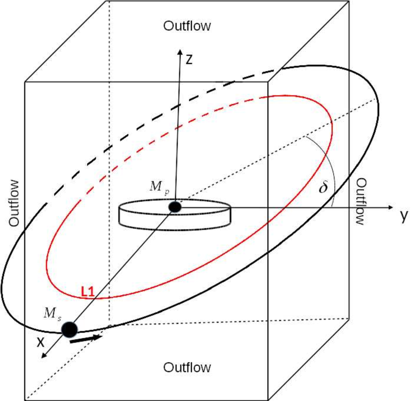
Figure 1.— Sketch of our model setup. We consider a binary system consisting of a primary of mass $M_{\rm p}$ surrounded by an accretion disk of size $r_{\rm out}$ and a secondary of mass $M_{\rm s}$. The Cartesian coordinate system originates in the primary. The orbital plane is inclined with an angle $\delta$ with respect to the initial accretion disk mid-plane. The secondary is located outside the computational domain, separated by a distance $D$ from the primary. The red circle displays the orbit of the inner Lagrange point L1 with respect to the primary. For a mass ratio $q\equiv M_{\rm s}/M_{\rm p}$ of unity, the L1 is located halfway between the two stars.

3. Model approach for jets from binary systems

We consider a binary system with a primary of mass $M_{\rm p}$ and a secondary of mass $M_{\rm s}$, separated by the distance $D$. The primary is surrounded by a disk of initial size $r_{\rm out}$. The location of the secondary is chosen to be outside the computational domain. The orbital plane of the binary system is inclined towards the initial accretion disk by an angle $\delta$. The Lagrange points L1, L2 and L3 are outside the initial disk radius. The Lagrange points L1 and L3 could be located in the computational domain, and even within the initial accretion disk depending on mass ratio and separation.

Figure 1 illustrates the general setup for our simulations of MHD jet launching from a circumstellar disk located in a binary system. The computational domain is shown by a rectangular box where we have indicated the inner Lagrange point L1 of the binary and the orbit of the secondary. The L1 point orbits with the secondary (red circle). In the present paper, we implement the full gravitational potential of the binary in the initially axisymmetric setup of the disk-jet. In other words, we take into account the orbital motion of the binary.

Since we choose the primary as the origin of the computational domain, we do not consider an inertial frame. The advance of this work compared to our previous paper (Sheikhnezami & Fendt, 2015) is that all tidal terms induced by the non-inertial frame are considered.

3.1. Magnetohydrodynamic equations

We apply the MHD code PLUTO (Mignone et al., 2007, 2012), version 4.0, to solve the time-dependent, resistive, in-viscous MHD equations, namely for the conservation of mass, momentum, and energy,

$$\frac{\partial\rho}{\partial t}+\nabla\cdot(\rho\vec{v})=0,$$ (1)

$$\frac{\partial(\rho\vec{v})}{\partial t}+\nabla\cdot\left(\vec{v}\rho\vec{v}-\frac{\vec{B}\vec{B}}{4\pi}\right)+\nabla\left(P+\frac{B^{2}}{8\pi}\right)+\rho\nabla\Phi=0,$$ (2)

Here, $\rho$ is the mass density, $\vec{v}$ is the velocity, $P$ is the thermal gas pressure, $\vec{B}$ stands for the magnetic field, and $\Phi$ denotes the gravitational potential.

The major advance of this paper is that we consider a time-dependent, three-dimensional gravitational potential $\Phi(x,y,z,t)$ that represents the Roche potential of a binary system (see Sect. 3.5).

The electric current density $\vec{j}$ is given by Ampére’s law $\vec{j}=(\nabla\times\vec{B})/4\pi$. The magnetic diffusivity is defined most generally as a tensor $\bar{\bar{\eta}}$. In this paper, for simplicity we assume a scalar, isotropic magnetic diffusivity $\eta_{ij}\equiv\eta(x,y,z)$ (see Section 3.2.). The evolution of the magnetic field is described by the induction equation,

$$\frac{\partial\vec{B}}{\partial t}-\nabla\times(\vec{v}\times\vec{B}-\eta\vec{j})=0.$$ (3)

The cooling term $\Lambda$ in the energy equation can be expressed in terms of ohmic heating $\Lambda=g\Gamma$, with $\Gamma=({\eta}\vec{j})\cdot\vec{j}$, and with $g$ measuring the fraction of the magnetic energy that is radiated away instead of being dissipated locally. For simplicity, again we adopt $g=1$, thus we neglect ohmic heating for the dynamical evolution of the system. The total energy density is

$$e=\frac{P}{\gamma-1}+\frac{\rho v^{2}}{2}+\frac{B^{2}}{2}+\rho\Phi.$$ (4)

The gas pressure follows a polytropic equation of state $P=(\gamma-1)u$ with $\gamma=5/3$ and the internal energy density $u$.

3.2. Magnetic diffusivity

Considering resistivity is essential for jet launching simulations (Casse & Keppens, 2002; Zanni et al., 2007; Murphy et al., 2010; Sheikhnezami et al., 2012; Fendt & Sheikhnezami, 2013; Stepanovs & Fendt, 2014, 2016). Accretion of disk material across a large-scale magnetic field that is threading the disk can only happen if that matter can diffuse across the field. After some time an equilibrium situation will be established between inward advection of magnetic flux along the disk and diffusion of flux in outward direction (see e.g. Sheikhnezami et al. 2012). Essentially, the launching of an outflow is a consequence from re-distributing matter across the magnetic field, and therefore depends strongly on the level of magnetic diffusivity.

In previous works, we have investigated in detail how the dynamics of the accretion-ejection structure - for example the corresponding mass fluxes, the jet rotation, or the jet propagation speed - depends on the profile and the magnitude of magnetic diffusivity (Sheikhnezami et al., 2012; Fendt & Sheikhnezami, 2013). These papers have typically applied a magnetic diffusivity $\eta=\eta(r,z)\propto h(r,z)$ that is constant in time and follows a Gaussian vertical profile $h(r,z)$, essentially parameterized by the the disk thermal scale height $H$.

When we extended our approach to 3D simulations (Sheikhnezami & Fendt, 2015), we found, however, that such a diffusivity profile may lead to instabilities in the 3D evolution of the system. The most stable and smooth evolution of the accretion-ejection structure we observed when applying a constant background diffusivity (as e.g. applied by von Rekowski et al. 2003). Therefore, we have followed this approach also for the present paper, and prescribe a constant level for the magnetic diffusivity inside the disk and for the nearby disk corona,

$$h(z)=\begin{cases}\eta_{0},&{\rm for}\quad|z|<10,\\ 0,&{\rm for}\quad|z|>10,\end{cases}$$ (5)

while we assume ideal MHD for the rest of the grid. We choose $\eta_{0}=0.03$ for all simulations presented here. We note that the very mass flux rates and other dynamical variables may depend on the exact diffusivity profile, however, a comparison between simulations applying the same diffusivity profile can of course be made.

Table 1Characteristic parameters of our simulation runs. Here, $\beta_{\rm i}$ is the initial (maximum) plasma-beta at the inner disk radius, $D$ is the binary separation (in the orbital plane), $\delta$ is the inclination angle between the binary orbit and the initial accretion disk mid-plane, $q\equiv M_{s}/M_{p}$ is the mass ratio between secondary and primary, $L1$ and $L3$ denote the radial location of the Lagrange points (in the orbital plane), $T_{\rm b}$ indicates the orbital period (in time units $t_{\rm i}$), and $r_{\rm out}=65$ is the initial outer radius of the disk. All values are given in code units.

Run	$\beta_{\rm i}$	D	$\delta$	$q$	$L1$	$L3$	$T_{\rm b}$
d150a0	20	150	0	1	75	-105	8162
d150a30	20	150	30	1	75	-105	8162
d150a10	20	150	10	1	75	-105	8162
d150m0.5	20	150	10	0.5	86	-120	9424
d150m2	20	150	10	2	64	-87	6664
d200a30	20	200	30	1	100	-140	12566
hydro	$10^{7}$	150	10	1	75	-105	8162
*The hydro simulation applies a very weak magnetic field

3.3. Numerical setup

Our simulations are performed in 3D Cartesian coordinates $(x,y,z)$. Note that contrary to our previous axisymmetric simulations, the $z$-axis is not a symmetry axis anymore. The computational domain typically extends over $x\in[-80,80]$ and $y\in[-80,80]$ in units of the inner disk radius $r_{\rm i}$ but has different extent in vertical direction $z$.

Cartesian coordinates may cause problems when treating rotating objects (see Sheikhnezami & Fendt 2015). Spherical coordinates are well suited for 3D disk simulations (see e.g. Flock et al. 2011; Suzuki & Inutsuka 2014), in particular if the region along the vertical axis is not considered. However, when investigating the 3D structure of a jet, artificial symmetry constraints by the rotational axis boundary conditions must be avoided.

The origin of the coordinate system is located in the primary. The $z$ axis is chosen to be along the rotation axis of the unperturbed disk. The accretion disk mid-plane initially follows the $x-y$ plane for $z=0$. We prescribe the orbital motion of the binary in a plane which has the inclination angle $\delta$ with respect to the initial accretion disk mid-plane. We denote the orbital angular velocity of the secondary around the primary with $\omega$, equivalent to the orbital angular velocity of the binary considering the center of mass.

We apply a uniform grid of $200\times 200\times 200=8\times 10^{6}$ cells for the very inner part of the domain, $-5.0<x,y,z<5.0$, in order to optimize the numerical resolution in the jet launching area. This corresponds to a resolution of about 20 cells per disk scale height ($\Delta x=\delta y=\delta z=0.05$). For the rest of the domain, i.e. the range $|\pm 5|<x,y,z<|\pm 80|$, we apply a stretched grid of $476\times 476\times 476$ grid cells. We apply a stretching factor of about 1.01. We also require that the shape of the grid cells is only moderately stretched, avoiding ill-defined cell aspect ratios that will limit the convergence of the numerical scheme.

The same normalization as in Sheikhnezami & Fendt (2015) is applied. Distances are expressed in units of the inner disk radius $r_{\rm i}$, while $P_{\rm d,i}$ and $\rho_{\rm d,i}$ are the disk pressure and density at this radius, respectively. Velocities are normalized in units of the Keplerian velocity $v_{\rm K,i}$ at the inner disk radius. We adopt $v_{\rm K,i}=1$ and $\rho_{\rm d,i}=1$ in code units. The pressure is given in units of $P_{\rm d,i}=\epsilon^{2}\rho_{\rm d,i}v_{\rm K,i}^{2}$. Here, $\epsilon$ is the ratio of the isothermal sound speed to the Keplerian speed, both evaluated at disk mid-plane, $\epsilon\equiv{c_{\rm s}}/{v_{\rm K}}$. The magnetic field is measured in units of $B_{\rm i}=B_{z,\rm i}$ where $B_{\rm i}=\epsilon\sqrt{2/\beta}$ with the plasma-beta $\beta$ as the ratio of the thermal to the magnetic pressure.

The dynamical time unit for the simulation is defined by the Keplerian speed at the inner disk radius, $t_{\rm i}=r_{\rm i}/v_{\rm K,i}$. Therefore, $t_{\rm i}=T_{\rm K,i}/2\pi$ with the Keplerian period of the disk at the inner disk radius, $T_{\rm K,i}=2\pi$ in code units.

We apply the method of constrained transport (CT) for the magnetic field evolution conserving $\nabla\cdot B$ by definition. For the spatial integration we use a linear algorithm with a second-order interpolation scheme, together with the third-order Runge–Kutta scheme for the time evolution. Further, a HLL Riemann solver is chosen.

3.4. Initial and boundary conditions

We apply the same initial conditions and boundary conditions as in Sheikhnezami & Fendt (2015). We prescribe an initially geometrically thin disk with the thermal scale height $H$ and $\epsilon=H/r=0.1$. The disk is supposed to be in vertical equilibrium between the thermal pressure and the gravity of the primary.

The initial disk density distribution is

$$\rho_{\rm d}=\rho_{\rm d,i}\left(\frac{2}{5\epsilon^{2}}\left[\frac{r_{i}}{R}-\left(1-\frac{5\epsilon^{2}}{2}\right)\frac{r_{i}}{r}\right]\right)^{3/2},$$ (6)

while for the initial disk pressure distribution we apply

$$P_{\rm d}=P_{\rm d,i}\left(\frac{\rho_{\rm d,i}}{\rho_{\rm d}}\right)^{5/3}.$$ (7)

Here, $r=\sqrt{x^{2}+y^{2}}$ and $R=\sqrt{x^{2}+y^{2}+z^{2}}$ denote the cylindrical and the spherical radius, respectively. The accretion disk is set into a slightly sub-Keplerian rotation accounting for the radial gas pressure gradient and advection and the non-force free structure of the magnetic field, initially.

The initial magnetic field distribution is prescribed by the magnetic flux function $\psi$,

$$\psi(x,y,z)=\frac{3}{4}B_{\rm z,i}r_{\rm i}^{2}\left(\frac{r}{r_{\rm i}}\right)^{3/4}\frac{m^{5/4}}{{\left(m^{2}+\left({z}/{r}\right)^{2}\right)}^{5/8}},$$ (8)

where the parameter $m$ determines the magnetic field bending (Zanni et al., 2007). In our model setup $m=0.4$. Here, $B_{z,\rm i}$ denotes the vertical magnetic field at the inner disk radius, $(r=r_{\rm i},z=0)$. Numerically, the poloidal field components are implemented by prescribing the magnetic vector potential $A_{\phi}(x,y)=\psi/r$. Initially $B_{\phi}=0$.

Above and below the disk, we define a density and pressure stratification that is in hydrostatic equilibrium with the gravity of the primary, a so-called ”corona”,

$$\rho_{\rm c}=\rho_{\rm a,i}\left(\frac{r_{\rm i}}{R}\right)^{1/(\gamma-1)}\!,\,P_{\rm c}=\rho_{\rm a,i}\frac{\gamma-1}{\gamma}\frac{GM}{r_{\rm i}}\left(\frac{r_{\rm i}}{R}\right)^{\gamma/(\gamma-1)}\!.$$ (9)

The parameter $\xi\equiv\rho_{\rm a,i}/\rho_{\rm d,i}$ quantifies the initial density contrast between disk and corona. In this paper $\xi=10^{-4}$. This initial density distribution is rather stable inside the Roche lobe of the primary. This is essential, as it allows for initial jet formation that is mainly unaffected by coronal motion. When the jet is launched, the coronal region becomes mass loaded by the outflow and is not affected anymore by the initial state. Note however, that a mass accumulation may happen at certain areas in the Roche volume (e.g. around the L4 and L5 point).

We prescribe a Keplerian rotation for the matter that crosses the inner boundary. The rotational velocity profile of the accretion disk is given by

$$v_{\phi}(r)=\sqrt{\frac{GM}{r}}\begin{cases}0,&{\rm for}\,\,0<r<r_{0}\\ \sqrt{1-5\epsilon^{2}},&{\rm for}\,\,r_{0}<r<r_{\rm i}\\ \sqrt{1-2.5\epsilon^{2}},&{\rm for}\,\,r_{\rm i}<r<r_{\rm out}\\ 0,&{\rm for}\,\,r>r_{\rm out}\end{cases}$$ (10)

where $r_{\rm i}$ denotes the inner disk radius and $r_{0}$ the inner radius of the ghost area corresponding to the inner boundary condition.

In our simulations the initial outer disk radius $r_{\rm out}$ is smaller than the size of the computational domain. The advantage of this prescription is that due to the weak disk rotation for large radii, no specific treatment is required at the outer grid boundary, in particular if the disk radius is smaller than the size of the computational domain. The disadvantage is that the mass reservoir for accretion is limited by the finite disk mass. This may constrain the running time of the simulation as soon as the disk has lost a substantial fraction of its initial mass (Sheikhnezami & Fendt, 2015).

However, since it is essential to treat the accretion process properly, we cannot use a similar strategy for the inner boundary and just neglect rotation over there. We thus make use of the internal boundary option of PLUTO and define the boundary values in a way that allows to absorb the disk material and its angular momentum and that ensures an axisymmetric rotation pattern in the innermost disk area (see Sheikhnezami & Fendt 2015, appendix).

For the outer boundaries of the computational domain, standard outflow conditions are applied as prescribed by PLUTO.

The orbital period of the binary $T_{\rm b}$ is defined as

$$T_{\rm b}=2\pi\sqrt{\frac{|D|^{3}}{G(M_{\rm p}+M_{\rm s})}},$$ (11)

and the orbital angular velocity as

$$\omega=\sqrt{\frac{G({M_{\rm p}+M_{\rm s})}}{|D|^{3}}},$$ (12)

where $D$ is the binary separation. For example, the orbital period of the binary system for run d150a0 with a binary separation of $D=150$ is $T_{\rm b}\simeq 8160$ dynamical time steps.

3.5. A time dependent gravitational potential

The gravitational potential of a binary system is the well-known Roche potential. The outflows will be launched deep within the Roche lobe of the primary star. When the outflow propagates away from the launching area, it becomes more and more affected by the tidal forces of the Roche potential, and will finally leave the Roche lobe of the primary.

Since the origin of our coordinate system is in the primary, we have to consider the time variation of the gravitational potential in that coordinate system. Below we describe the total gravitational potential that is affecting a mass element in the binary system (see Figure 1). Assuming that the position of the secondary at $t=0$ is within the $x$-$z$ plane, its position vector is

$$\vec{D}=\hat{x}D\cos{\omega t}+\hat{y}D\sin{\omega t}\cos{\delta}+\hat{z}D\sin{\omega t}\sin{\delta}.$$ (13)

The effective potential in a binary system at a point with position vector $\vec{r}(x,y,z)$ is

$$\Phi_{\rm eff}=-\frac{GM_{\rm p}}{|\vec{r}|}-\frac{GM_{\rm s}}{|\vec{r}-\vec{D}|}+\frac{GM_{\rm s}}{|\vec{D}|^{3}}\left(\vec{r}\cdot\vec{D}\right).$$ (14)

The first term in Equation 14 is the gravitational potential of the primary, while the remaining terms describe the tidal perturbations due to the orbiting secondary. These equations have been used previously by other theoretical studies (see e.g. Papaloizou & Terquem 1995; Larwood et al. 1996; Fragner & Nelson 2010). We notice again that the reference frame for our simulations is not an inertial frame and that the last term in Equation 14 - usually denoted as indirect term - accounts for the acceleration of the origin of the coordinate system.

The motion of masses that are moving in the binary system are governed by the total (effective) gravitational potential. From the five Lagrange points that exist, three of them ($L1,L2,L3$) are meta-stable points, while the other two ($L4,L5$) are truly stable points. In the meta-stable points a small perturbation to a mass distribution element will lead to instability. We therefore expect to see specific imprints in the dynamical evolution of the disk and the outflow when these constituents approach or pass the Lagrange points or the Roche lobe. Note that in our coordinate system (centered on the primary) the Lagrange points orbit with the orbital frequency of the binary.

3.6. Limits of our model approach

Here we discuss the limits of our model approach. First of all, we point out that the main aim of the paper is to investigate the jet launching from a circum-stellar disk that is located in a binary system. Our main aim is not to model a binary system as such. The binary system provides the background gravity for jet launching. Our simulations can be seen as complementary to a large number of studies considering hydrodynamical models and simulations of disks in binary stars (see e.g. Artymowicz & Lubow 1994; Larwood et al. 1996; Terquem et al. 1999 for early modelling, and Kley et al. 2008; Nixon et al. 2013; Picogna & Marzari 2015; Bowen et al. 2017 for more recent simulation work). Without the need of considering the magnetic field and a computational domain that allows for jet propagation, these simulations reach much longer physical times, as of now up to 100s of orbital periods (see e.g. Kley et al. 2008; Fragner & Nelson 2010; Müller & Kley 2012).

Jet launching implies the necessity of MHD and a large vertical grid extension, while the binarity implies a fully 3D approach. As a result, these simulations are numerically expensive, running two months per parameter run on 256 cores corresponding to $\simeq$ 5000 processors.

With the computational resources and a suitable time frame at hand, we are able to run the simulations about 5000 physical time steps corresponding to about 1000 revolutions of the inner disk. This is indeed sufficient to follow the jet formation process from inner disk, as the typical jet dynamical time scale roughly corresponds to the Keplerian time at the launching point. This enables us to detect any changes in the propagation characteristics of the inner jet easily. Such a change could indicate a hypothetical jet precession when the jet source moves along its orbit. The 5000 dynamical time units that defined by the inner disk rotation correspond, however, ”only” to about half a binary orbit for the chosen separation and mass ratio.

It is known, however, that tidal effects are expected to have fully evolved only after some binary orbital times (see e.g. Larwood et al. 1996; Kley et al. 2008; Müller & Kley 2012). Thus, in order to be able to see any indication for tidal effects, we have to shrink the binary to a suitable size. Here, we apply a binary separation of 150-200 inner disk radii.

This separation corresponds to about 15-20 AU for young stars, or about 2000-3000 Schwarzschild radii for a neutron star disk (see Table 2). While these values are consistent with some of the observed sources, as for example Gliese 86 (Queloz et al., 2000), Gamma Cephei (Campbell et al., 1988), HD 196885 (Correia et al., 2008), or microquasars such as SS433 (Gravity Collaboration et al., 2017), we do not (and we cannot) intend to model specific observed systems.

Table 2Physical scaling of examples of potential binary jet sources, based on our model setup applying a binary separation $D=150-200r_{\rm i}$. Here, $R*$ is the radius of the star, $R_{\rm in}$ is the inner disk radius, and $R_{\rm S}$ is the Schwarzschild radius. Naturally these values depend also on the masses of the binary components.

Source	$R_{\rm in}$	$D$
Young stellar objects	$3R*\simeq$ 0.1 AU	15 - 20 AU
Cataclysmic variables	$3R*\simeq 2000R_{\rm S}$	$30.000-40.000R_{\rm S}$
Neutron star binaries	$3R*\simeq 15R_{\rm S}$	$2.000-3.000R_{\rm S}$

We note that within our model approach the choice of stellar separation and the initial disk radius also puts a constraint on the available disk mass reservoir. The disk looses mass by accretion and ejection, and without replenishing the mass that is lost, the disk will disappear after about one orbital time (in our setup). We have therefore applied a disk as large as possible, meaning being constraint only by the Roche sphere. This might be in slight contradiction with classical papers (Papaloizou & Pringle, 1977; Paczynski, 1977; Artymowicz & Lubow, 1994), however, the difference in size is only a factor of two. Later studies although applying a different mass ratio also apply larger disks (Truss, 2007; Pichardo et al., 2005; Müller & Kley, 2012).

4. Results and discussion

We now present the results of simulations runs that apply a different binary separation, a different inclination between the initial accretion disk mid-plane and the binary orbital plane, or a different binary mass ratio (see Table 1).

The major advance to our previous paper (Sheikhnezami & Fendt, 2015) is that we now consider a 3D time-variable gravitational potential. We thus take into account the tidal effects of the secondary ”orbiting” the jet source. All simulation runs have been performed for a considerable fraction of the binary orbital period, the latter corresponding to more than 5000 dynamical time steps, depending on mass ratio and binary separation.

For comparison we have run also a simulation in the hydrodynamic limit that serves as a test case for the initial disk structure. The disk remains stable over several 100s rotational periods until 3D tidal effects disturb the initial structure. As expected, outflows could not be form by this setup.

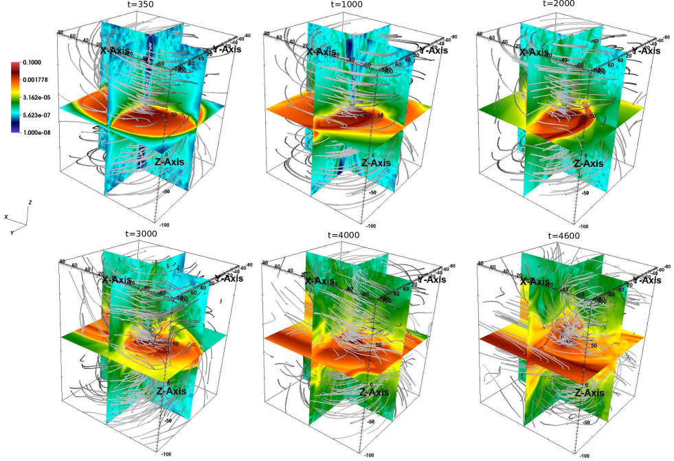
Figure 2.— Three-dimensional evolution of simulation run d150a0 with binary separation $D=150r_{\rm i}$ and no inclination between the disk and the binary orbital plane. Shown are slices of the mass density (color bar) at times $t=530,1000,2000,3000,4000,4600$ and magnetic field lines (grey).

4.1. Co-planar orbital planes

We first discuss simulation run d150a0 with an orbital plane co-planar to the initial disk plane. We consider this run as reference run and will compare it with the simulations applying an inclined binary orbit and also to the 2D simulations we have published earlier. This run lasted for about 5000 dynamical times.

The global evolution is shown in Figure 2 where we plot three-dimensional slices of the mass density for times $t=530,1000,2000,3000.4000,4600$, over-plotted with field lines. We clearly see that a well structured and continuous outflow is launched from the disk. The disk, the jet and the magnetic field evolve rapidly and change from a smooth structure to a rather disturbed pattern. The details of the evolution is seen better in 2D slices of the simulation. Figures 5, 5 and 5 show slices of the mass density in the $x$-$z$ plane, the $y$-$z$ plane and the $x$-$y$ plane, respectively. The ”$+$” symbol indicates the (projected) position of the inner Lagrange point $L1$ at each time.

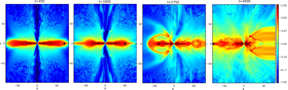
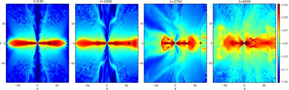
Figure 3.— Reference simulation run d150a0 with binary separation $D=150r_{\rm i}$ and no inclination between the disk and the binary orbital plane. Shown are two dimensional slices of the mass density in the $x$-$z$ plane for $t=530,1000,2750,4000$. The “$+$”symbol indicates to the location of the inner Lagrange point L1 of the binary system projected into $x$-$z$ plane.

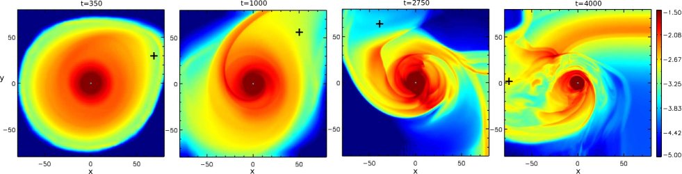
Figure 4.— Same as Figure 5, but for the $y$-$z$ plane.

Figure 5.— Same as Figures 5 and 5, but for the $x$-$y$ plane (initial equatorial plane of the accretion disk).

We find that the initial pattern of both the disk and the jet is symmetric to a high degree, again demonstrating the quality of the initial setup and of the inner boundary conditions. However, over long time, i.e. a substantial fraction of the orbit time, the symmetry of the system weakens substantially.

Essentially, the upper and lower hemisphere evolve symmetrically with respect to the equatorial plane. As the secondary moves in the disk mid-plane, it induces an asymmetry only in horizontal direction (it moves from right to left around the vertical axis of the coordinate system in Figures 5 and 5). Since the binary orbital plane and the accretion disk are co-planar, the material in the upper and lower hemisphere feels the same tidal forces. Overall, this leads to a hemispherically symmetric evolution of the system.

In contrary, the ”left” and ”right” hemispheres feel different tidal forces, which leads to an asymmetric evolution in these hemispheres. This can clearly be seen by comparing the left and right part of the computational domain for the snapshots taken at different time (in either $x$-$z$ or $y$-$z$ slices). Essentially, the asymmetry is visible for both the disk structure and the outflow.

The slice in the disk mid-plane shows further interesting features (Figure 5). Prominently visible are the ”spiral arms” that start forming at time $t=500$ and essentially grow from outside to the inside. At time $t=2000$ a clear two-arm structure of the outer disk has developed, and a third arm is just forming. This point in time corresponds to about 320 inner disk revolutions, corresponding to a quarter of the binary orbital period. Around $t=2000$, the spiral arms extend down to about $r\simeq 30$.

At this radius the Keplerian period is only about $1000\,t_{\rm i}$, so disk material moving at this radius with Keplerian speed have performed two revolutions. We note that the sense of rotation is the same for the disk material, the spiral arm pattern, and also for the secondary.

Figure 5 shows how the initial disk becomes truncated. The disk radius at $t=1000$ is about half the radius of L1. This is consistent with the literature (Artymowicz & Lubow, 1994; Truss, 2007; Kley et al., 2008; Müller & Kley, 2012; Daemgen et al., 2013; Picogna & Marzari, 2015; Miranda & Lai, 2015; Ju et al., 2017). In all these works the tidal truncation happens inside the Roche lobe. Depending on the disk physics applied (these papers were mostly dealing with hydrodynamics and were considering viscosity) the truncation radius is typically 0.4-0.5 the binary semi-major axis (Paczynski, 1977; Artymowicz & Lubow, 1994; Blondin, 2000). We note that the mass located outside the Roche lobe is lost for accretion to the primary, and also for ejection as a jet.

The dynamical evolution we have discussed for the disk structure is partly seen also in the outflow. In particular, we mention the jet material that is passing the Roche lobe in vertical direction. Clearly, this material is more and more affected by the gravity of the secondary. As a consequence, it changes its path of motion away from the initial direction of ejection.

Since for this simulation the binary orbit is co-planar with the accretion disk, we do not see any changes in the disk alignment. As the jet is ejected from the inner disk also, we also do not see a change in the jet rotational axis. However, as discussed just above the jet dynamics evolves towards a left-right asymmetry, being affected by the tidal forces of the binary.

4.2. A highly inclined orbit

We now consider run d150a30 with a binary separation is $D=150$ and an initial inclination between accretion disk and binary orbit of $30\arcdeg$. This run serves as an extreme case with both a large inclination angle and a small separation. We therefore expect a rapid evolution of non-axisymmetric effects for the disk and the jet.

We have performed this simulation for 4500 dynamical time steps corresponding to more than half of the binary orbital period. As mentioned above, the simulation run time is limited by the mass reservoir of the disk, as the disk mass is depleted by accretion and ejection. Due to the small disk radius (limited by the L1), also the initial disk mass is small, and does not allow for a much longer simulation time (see our discussion in Section 3.6).

Although it would be possible in principle to compensate the mass loss by mass injection, such a procedure may break the initially axisymmetric evolution by construction. Therefore, we do not apply such a procedure in the current study. Nevertheless, run d150a30 does last long enough in order to develop a number of asymmetric features that evolve in the disk/jet system.

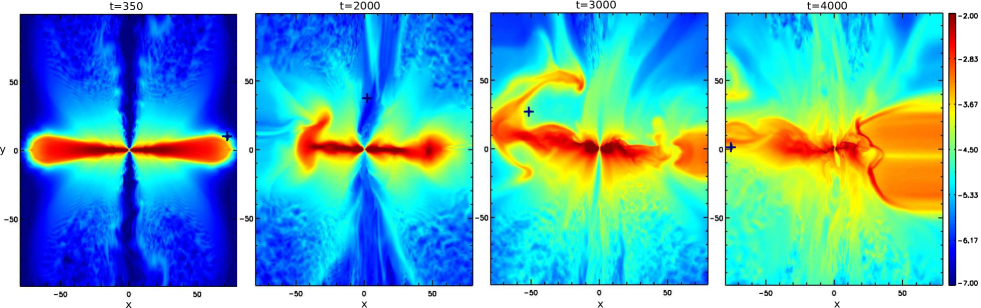
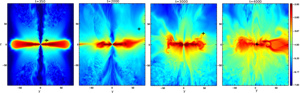
Figure 6.— Simulation run d150a30 with binary separation $D=150r_{\rm i}$ and $30\deg$ inclination between the disk and the binary orbital plane. Shown are two dimensional slices of the mass density in the $x$-$z$ plane for $t=350,2000,3000,4000$. The “$+$”symbol indicates to the location of the inner Lagrange point L1 of the binary system projected into $x$-$z$ plane.

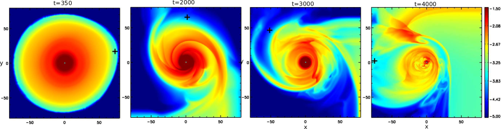
Figure 7.— Same as Figure 8, but for the $y$-$z$ plane.

Figure 8.— Same as for Figures 8 and 8 but for the $x$-$y$ plane at $z=0$ (initial accretion disk mid-plane) and for times $t=350,1040,2000,3000,4000,4500$. Note that at times $t=1000,3000$ the L3 point is located at distance $r\simeq 75$ from the origin just inside the lower left (right) corner.

In Figures 8 and 8 we show slices of mass density in the $x$-$z$ plane and in the $x$-$y$ plane for simulation run d150a30 at different time. We find that after about 500 dynamical time steps a global, 3D non-axisymmetric pattern evolves from the symmetric initial setup. The disk-jet system evolves rapidly, so that after about $t=2500$ the disk structure has completely changed.

We first discuss the disk evolution, focusing on the disk area only (see Figure 8). We note that the initial disk has a axisymmetric structure and is also symmetric in both hemispheres.

When we start the simulation, the secondary is located at position $(x=150,y=0,z=0)$ and reaches the position $(x=0,y=129,z=75)$ after a quarter of an orbit. Thus, the L1 is initially located at $(x=75,y=0,z=0)$. After time $t\simeq 500$ the symmetry of the system is slightly broken. The is visible e.g. in Figure 9 where we show a volume rendering of the disk mass density in the $x$-$y$ plane. Overall we see the formation of spiral arms forming in the disk and a disk structure that is not smooth anymore.

In difference to our previous work we see the spiral pattern rotating with the sense of the disk rotation and the orbital motion. In the previous paper with a fixed gravitational potential and considering shorter simulation times, a spiral pattern was initiated, but it was not rotating. The present result is consistent with the orbital motion of the secondary and reflects the effect of the time-varying effective gravitational potential implemented in the model.

After $t\simeq 2500$ we see the outer part of the disk beginning to inflate. The inflated part of the disk is growing in size and is clearly seen at later evolutionary stages $t>4000$ (Figure 9). We believe that this inflation arises from the fact that the outer disk is located close to the Roche lobe. As a consequence, it is strongly affected by tidal forces that will destroy the initially Keplerian disk structure. Also the vertical gravitational forces are weaker in comparison to a Keplerian disk, so the gas pressure initially prescribed for the disk will be able to expand the disk easily.

This evolution is similar to that we show in the previous section for the simulation with co-planar orbits. However, here, the disk stability is even more disturbed by tidal forces due to the higher inclination of orbital plane. Thus, apart from these effects that arise from the local force-balance, also the global dynamical disk structure will be perturbed giving rise to warps in the disk.

Our results concerning the circum-stellar disk evolution are in agreement with previous hydrodynamical simulations of binary systems, also considering a misalignment between the disk and the binary orbit (see e.g. Larwood et al. 1996; Fragner & Nelson 2010; Nixon et al. 2013; Picogna & Marzari 2015). These works investigate the disk stability and the conditions under which the inclined disk may undergo a rigid precession or does form disk warps. Larwood et al. (1996) find warps and a rigid precession in an inclined thin disk within a binary system and, in particular, that a very thin disk may be severely disrupted by differential precession, and therefore cannot survive. Similarly, Fragner & Nelson (2010) study how the detailed disk structure that arises in a misaligned binary system depends on disk parameters as viscosity or disk thickness and investigate the conditions that lead to an inclined disk that may be disrupted by strong differential precession. In particular, they find that for a disk thickness $h=0.05$ the warp that forms effectively allows the disk to precess as a rigid body with little twisting. These disks seem to align with the binary orbital plane on a viscous evolution time. Thinner disks of higher viscosity develop significant twists before achieving rigid-body precession.

In our simulations we observe the clear impact of the tidal forces on the disk evolution that lead to asymmetric features like warps and even in some cases lead to a disk disruption - in agreement with the literature, but now investigated for jet launching MHD disks.

In Figures 8 and 8 we observe that at later evolutionary stages a flow of low density material establishes outside the Roche lobe (but close to the disk plane), and then moves inwards where it is obviously disturbing the disk structure and the existing spiral arm pattern. We believe that this flow is caused by the combination of effects.

Firstly, the spiral arms are growing and thus affecting a larger area inside the disk structure probably because the inner disk becomes lighter and lighter with time as loosing mass due to accretion and ejection. Secondly, the disk is inflating in the outer part (in particular close to the L1) and this part of the disk mass will be loaded into the area outside the Roche lobe. The further dynamics of this flow is then determined by the effective potential of both stars, eventually resulting in the flow structure we just observe. It is, unfortunately, impossible to predict analytically the dynamics of such a flow. But as the code considers the full MHD dynamics of the flow we are confident that the flow structure we observe is in fact a physical effect.

In summary, we think that the combination of warp formation inside the disk in connection with the orbital motion of the secondary (disk inflation) results in forming a flow of matter out of the outer part of the disk that is filling the space around the disk. Jet launching is initially not affected, but when the launching source - the disk - becomes weaker with time, also jet formation is suppressed.

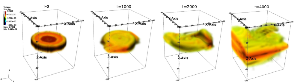
Figure 9.— Disk evolution for simulation run d150a30 considering a highly inclined orbital plane. Shown is the 3D volume rendering of the mass density (threshold $\rho>10^{-4}$).

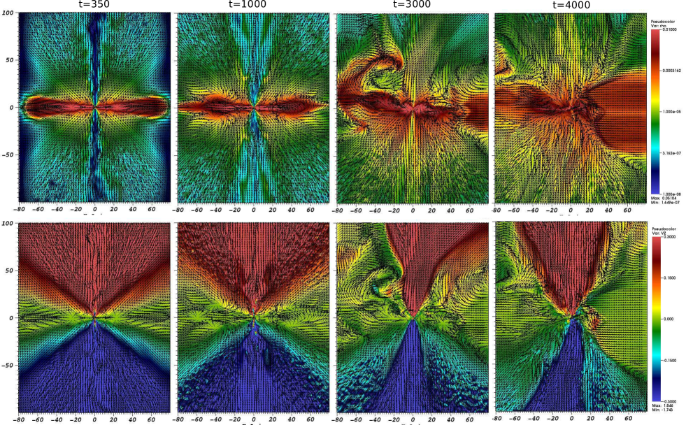
Figure 10.— Poloidal velocity maps. Shown are two dimensional slices of the vertical velocity $|v_{z}|$ (top) and the mass density (bottom) in the $x$-$z$ plane for run d150a30 at time $t=350,2000,3000,4000$. The arrows indicate the (normalized) velocity vector field of the $\vec{v}_{p}$ projected in $x$-$z$ plane.

Like the disk, also the jet undergoes a rapid time evolution. Figure 10 shows 2D slices of the vertical velocity $v_{z}$ (top) and the mass density (bottom) in the $x$-$z$ plane for simulation d150a30 at time $t=350,2000,3000,4000$. In addition the arrows are indicating to the velocity vector field projected in $x$-$z$ plane. Note that the blue central spine in the upper-left panel is not the jet. The jet-wind is launched from all over the disk surface is constitutes of the ”yellow-green” material (representing low velocities) close to the disk, that is ejected and accelerated to large distance from the disk surface.

We find that a strong and axisymmetric bipolar jet is formed during the early evolution. For $t>1500$ we see that the jet propagation starts to deviate from its initial straight motion that is perpendicular to the initial disk plane. The direction of jet propagation is influenced by two effects. Firstly, the accretion disk, thus the jet source, aligns towards the binary orbital plane. Therefore, as a consequence, the direction into which the jet is launched changes as well. We find that the deviation from the alignment with the initial rotational axis increases with time. Secondly, the jet direction of propagation is affected by the global tidal forces, thus the orbital motion of the secondary. These tidal forces of the binary system will influence the jet propagation more and more when it is propagating further away from the launching point, in particular, when the jet leaves the Roche lobe of the primary.

Essentially, we find that at late evolutionary stages both the accretion and the ejection pattern is disrupted and no outflows should be expected from such kind of launching geometry with a large inclination between disk and orbital plane.

4.3. Impact of the (initial) inclination angle

We now consider additional simulation runs and compare the disk and jet evolution for different initial inclination angle.

Binary orbits that are inclined against the disk mid-plane has been studied previously. For example Papaloizou & Pringle (1983) and Papaloizou et al. (1997) have studied a non-planar disk in close binary system analytically, whereas Fragner & Nelson (2010) applied hydrodynamical simulations in order to study the detailed structure and evolution of disks in misaligned binary systems. However, jet launching or disk winds were not considered in this work.

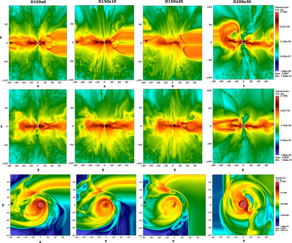
Figure 11.— Comparison of the four simulation runs d150a0, d150a10, d150a30, and d200a30 (from left to right) applying different initial inclination between the disk plane and the orbital plane and a different binary separation. Shown are 2D slices of the mass density in the $x$-$y$ , $x$-$z$ and $y$-$z$ plane (from top to bottom) around time $t=4000$. See Table 1 for the simulation parameters.

We first consider the mass density distribution in different runs at a specific, late evolution time. Figure 11 shows 2D slices of the mass density distribution in the $x$-$z$ , $y$-$z$ and $x$-$y$ plane, around $t=4000$ for different runs applying a mass ratio of unity (see Table 1). The global evolution in all four runs clearly follows a similar pattern. However, we observe that in the cases considering a large initial inclination angle (the last two snapshots) the alignment of the disk changes strongly. In contrary, in run d150a10 with an initial inclination angle of $10\arcdeg$, the initial alignment of the disk mid-plane is only slightly changed over time. Note that while tidal forces on the disk are similar for different disk inclinations, the tidal torque is different, thus explaining our findings for the differences in disk alignment.

We further see that the deviation of the jet axis from its initial direction is larger in case of a larger initial inclination angle. Moreover, the internal structure of both the disk and the jet changes more over time. In particular, for run d150a30 the outflow launching mechanism is clearly stalled at late evolutionary stages, beyond which we do not detect any well structured bipolar jets. Essentially, we conclude that there exists a critical angle between the accretion disk and the binary orbit beyond which the launching of typical jet is suppressed by 3D tidal forces. For the simulation setup investigated here, the critical angle is between 20 and 30°.

It is interesting to note that all jet sources found so far carry a strong magnetic field and are surrounded by an accretion disks. However, no jets have been found for Cataclysmic Variables and are extremely rare for pulsars although both kind of systems may also have a strong magnetic field and also host an accretion disk (see for example Murray & Chiang 1996 or Silber et al. 1994 for disk accretion, or Wang et al. 2017 for the detection of a magnetic field).

Similar to cataclysmic variables, jet from neutron stars have not been observed in general. There are few exceptions such as the Vela pulsar (Durant et al., 2013) and, as mentioned above, SS 433. Also the Crab pulsar shows a time-variable, elongated feature that could be interpreted as a jet (Mignone et al., 2013).

In summary, (almost) no jets have been observed from these numerous and extremely well observed binaries (Knigge & Livio, 1998; Soker & Lasota, 2004). An explanation for this observational fact has been suggested by Fendt & Zinnecker (1998) who consider a certain degree of axisymmetry as essential ingredient for jet launching. Our present simulations support this idea.

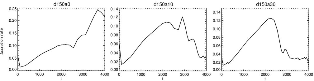
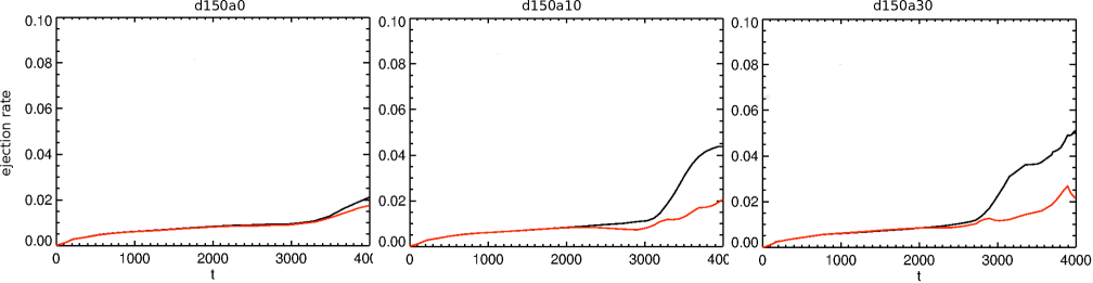
Figure 12.— Time evolution of the accretion mass flux. Shown are the mass fluxes in the disk integrated along $r=2$ and for three (initial) thermal scale heights $h$ for the simulation runs d150a0 (left), d150a10 (middle)and d150a30 (right).

Figure 13.— Time evolution of the bipolar outflow mass flux. Shown are the mass fluxes $\dot{M}$ for the jet (upper hemisphere; in red) and the counter jet (lower hemisphere, in black ) for the simulation runs d150a0 (left) d150a10 (middle) and d150a30 (right). The number values were integrated far from the disk at altitude $z=90$ .

A good way to quantify the launching efficiency and also the system asymmetry is to evaluate the mass fluxes in the disk and in the outflows. Figure 13 shows the the evolution of the disk accretion flux, integrated at disk radius $r=2$ over three (initial) thermal scale heights $H$ for the simulation runs d150a0, d150a10 and d150a30. Although in all cases the global evolution of the system looks similar, the simulation applying a co-planar orbit with the disk has on average a higher accretion rate. In all cases, the time evolution of the accretion flux peaks at later time steps. We understand this peak as due to the onset of 3D disk instabilities, the spiral wave, or warps that enhance the angular momentum transport and thus facilitate accretion.

Figure 13 shows the evolution of the ejected mass flux for jet and counter jet for the simulation runs d150a0 (top) d150a10 (middle) and d150a30 (bottom). We have integrated the asymptotic value for the outflow mass fluxes far from the disk at $z=\pm 90$. As a result, we observe that the vertical mass flux in both hemispheres is similar and only later the hemispheric symmetry is broken. It is strongly indicated that the asymmetry between the mass flux integrated in each hemisphere is higher for the simulation runs d150a10 and d150a30, thus runs those with an asymmetric initial setup. This is understandable as the hemispheric symmetry of the gravitational potential is broken by the secondary that is located initially in the upper hemisphere. We expect that when we would have been able to run our simulations over much longer time, e.g. several orbital periods, the average outflow mass flux in both hemisphere would be on average comparable.

4.4. Impact of the binary separation

We now consider additional simulation runs and compare the disk and jet evolution for a different binary separation.

In simulation run d200a30 - considering a larger binary separation-the L1 is located at 100$r_{\rm i}$ (outside the domain) and the orbital period of the binary is substantially longer, $T_{\rm b}=12,560t_{\rm i}$. This simulation was run for about 5000 dynamical time steps corresponding to about one third of the binary orbit.

In Figure 11 (last row) we show $x$-$y$ slices of the mass density distribution of run d200a30 that we can use to compare the disk structure and with its spiral arms to the other simulations. Clearly, the initial axisymmetric disk structure is disturbed by tidal forces as in the other runs. However, as these forces are weaker due to the larger separation, the disk looks more regular and ”roundish”. Compared to simulation d150a30 the inner disk is less dissolved (if we compare both disks for $r<10$). The ”roundish” part of the disk is also larger for the present simulation than for the simulations applying a smaller binary separation. This is as expected as L1 is now outside the computational grid.

Besides the weaker tidal forces, also the time scale after which we may identify tidal effects has increased as the orbital period is longer. We find a factor $\simeq 2$ for the increase of this time scale. Overall, the impact of tidal effects on jet launching critically depend on the binary separation.

In Figure 11 we observe a “warp” forming in the disk (see the snapshots of mass density in the $x$-$z$ and $y$-$z$ plane). These warps are only forming in simulations that start off with an initial inclination between the disk mid-plane and the binary orbit. The warps are stronger in simulation run d150a30 that applies the largest initial inclination angle and a small separation, thus reflecting a large tidal influence by the secondary.

4.5. Impact of the binary mass ratio

In order to investigate the impact of the binary mass ratio on the disk-jet dynamical evolution we have also run simulation with a mass ratio $M_{\rm s}/M_{\rm p}$ of 2 and 0.5, denoted as d150m2.0 and d150m0.5, respectively. The mass ratio obviously affects the size of the Roche lobe of the primary, thus the tidal forces on disk and jet, and the (orbital) time scale of the evolution (see Table 1).

In our setup, the orbital period of the binary increases, $T_{\rm b}=6664,8162,9424$, for decreasing mass ratio $M_{\rm s}/M_{\rm p}=2.0,1.0,0.5$, respectively. Therefore, to investigate the evolution of a low mass ratio system requires more CPU time. On the other hand, the tidal effects by a high mass secondary on a low mass jet source is expected to be higher, and thus to appear earlier with respect of the orbital period.

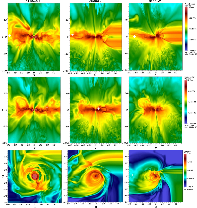
Figure 14.— Comparison of launching simulations with different binary mass ratio. Shown are 2D slices of the mass density in the $x$-$y$, $x$-$z$ and $y$-$z$ plane (from top to bottom) around time $t=4000$ for the three simulation runs d150m0.5, d150a10, d150m2 (from left to right). The “$+$”symbol indicates the projected location of the inner Lagrange point L1 (the L1 is located inside the domain for simulation d150m2).

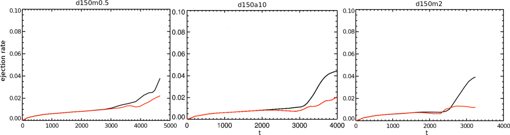
Figure 15.— Time evolution of the accretion mass flux. Shown are the mass fluxes in the disk integrated along $r=2$ and for three (initial) thermal scale heights $h$ for the simulation runs d150m0.5 (left), d150m2 (middle), and d150a10 (right), applying a different binary mass ratio.

Figure 16.— Time evolution of the bipolar outflow mass flux. Shown are the mass fluxes $\dot{M}$ for the jet (upper hemisphere; in red) and the counter jet (lower hemisphere; in black ) for the simulation runs d150m0.5 (left), d150a10 (middle), and d150m2 (right), applying a different binary mass ratio. The mass fluxes are integrated far from the disk at altitude $|z|=90$.

In Figure 14 we compare 2D slices of the mass density in the $x$-$y$, the $x$-$z$, and the $y$-$z$-plane (from top to bottom) at $t\simeq 4000$ for the three simulation runs d150m0.5, d150a10, d150m2 (from left to right) applying a different mass ratio. We find that the disk structure in run d150a0.5 is less disturbed in comparison with the disk in run d150m2 for which the disk has deviated from a round structure substantially and is also truncated at a smaller radius. This is clearly an effect caused by the larger tidal forces in run d150m2 with a large mass ratio $M_{\rm s}/M_{\rm p}=2.0$.

We find as well that the jet is more deflected from its original direction along the axis for the higher mass ratio (see in particular the $x$-$z$-slice ford150m2), and also that the deflection is stronger in the upper hemisphere in which the secondary is located.

We have also investigated the impact of the mass ratio on the global evolution of the system by considering the mass fluxes in the disk-jet structure. This is illustrated in Figure 16 showing the mass fluxes in the disk integrated at $r=2$ and for three (initial) thermal scale heights $h$ for the simulation runs d150a10 (left), d150m2 (middle) and d150m0.5 (right) applying different mass ratio.

Essentially, we find a delay in the accretion evolution of run d150m0.5 compared to other two runs. Also, the accretion rate in simulation d150m2 is slightly higher than for d150a10. This is probably due to the stronger and earlier formed spiral arms in the disk and thus a more efficient (tidal) angular momentum removal from the disk.

As for the accretion rate, in Figure 16 we compare the evolution of the ejected mass flux for jet (in red) and counter jet (in black). Here we find that the run d150m0.5 shows a weaker asymmetry in the outflow mass flux in the upper the and lower hemisphere compared to the other simulations. The explanation is similar as for the accretion rates. In simulation d150m0.5 the tidal forces of the secondary are weaker and cannot disturb the flow symmetry as much as for the other simulations.

4.6. Jet / disk precession?

The original motivation for these simulations was the question whether we can find indication for a disk or jet precession, similar to what the observations suggest (see Sect. 2).

Above we have discussed our findings that whenever a misalignment is present between the binary orbital plane and the (initial) disk plane, we observe a re-alignment of the disk and, as a consequence, subsequently also a re-alignment of the outflow axis. The question remains whether the re-alignment we observe will actually evolve into a constant precession of the disk and jet axis. Precession would imply an orbital motion of the jet axis around the initial jet axis (the z-axis) along a cone with a certain opening angle.

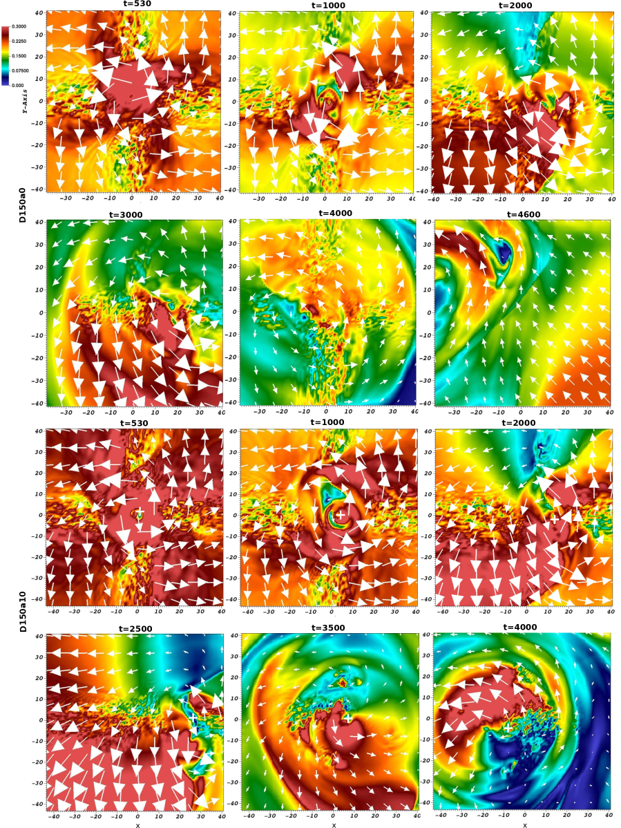
Figure 17.— Rotational evolution in the outflow. Shown are slices of the magnitude of the $x$-$y$ velocity, thus $\sqrt{v_{x}^{2}+v_{y}^{2}}$ (color) in the $x$-$y$ plane at $z=60$ for the two simulation runs d150a0 (upper two rows) and d150a10 (lower two rows) at different times. While this velocity pattern is dominated by the toroidal velocity in the outflow (rotation), a small contribution of the radial velocity of the outflow (projected in to the $x$-$y$ plane) cannot be disentangled (the main poloidal outflow component is vertical). The arrows indicate the velocity vector field projected into the plane. The “+” symbol illustrates the approximate position of the jet rotation axis.

Since our simulations consider all gravitational forces present in the system (the Coriolis force and the time-dependent gravitational potential), we could in principle find and prove a true precession of the disk and jet.

However, as already mentioned above, since precession evolves over several orbital time scales, a long run time of the simulation would be required. Typical estimates of the precession time scale of a disk in a binary system due to tidal forces is of the order of $T_{\rm P}\simeq 20T_{\rm b}$ (Bate et al., 2000).

This is of course a challenge considering a 3D MHD setup and the required numerical resolution. The typical running time scale of our simulations is about 4000-5000 dynamical time steps, corresponding to 20-30 years in case of YSOs or 7-10 years in case of AGN. This substantially less than the time scale needed for jet precession to evolve fully. Thus, we would only be able to indicate the onset of precession. Nevertheless, after half of an orbital period of the binary, corresponding to about 500 revolutions of the jet launching inner disk, we expect to see indication of a circular motion of the jet axis that is inclined against the original jet and disk rotational axis (at $t=0$), and thereby indication of a precession effect.

Figure 17 shows two dimensional slices of the projected velocity in the $x$-$y$ plane at $z=60$ for two runs d150a0 and d150a10. We plot the velocity magnitude (color-coded) and the velocity field (arrows). The panels consider simulations runs d150a0 (rows 1, 2 ), d150a10 (rows 3, 4 ), from top to bottom. Note that what is shown in Figure 17 is the projected velocity $\sqrt{v_{x}^{2}+v_{y}^{2}}=\sqrt{V_{r}^{2}+V_{\phi}^{2}}$ that is a superposition of the rotation and the radial flow (for example the radial outflow of the jet). It is well known that for classical MHD jets that are super-Alfvénic, $v_{\rm p}>>v_{\rm A}$, we have $v_{\rm p}>>v_{\phi}$, and that far from the source in a collimated jet we expect $v_{z}>>v_{r}$. Thus, we expect a (projected) radial outflow motion that is, however, not large. Thus, $v_{\phi}\simeq v_{r}$, implying that is difficult to disentangle orbital motion from radial motion in the jet.

After all, it is not straight forward to determine the exact position of the jet rotation axis. We estimate the approximate position of the jet axis considering the direction of the velocity arrows. In particular, close to the jet axis, the radial outflow speed is expected to be small compared to the vertical speed, thus the velocity vectors are related more to the rotational pattern than to the outflow pattern. Note, however, that due to the overall 3D gravitational potential and the fact that the the slice at $z=60$ is close to the Roche lobe, we may also expect a lateral bulk motion of the jet that could have a larger amplitude than the expected precession. If this is true, we would not be able to detect precession.

In Figure 17 we have applied the procedures just explained and have marked with a “+” symbol the approximate position of the jet rotation axis. Indeed, we clearly observe a feature indicating jet rotation and we also see a clear displacement of the jet rotational axis in time clearly in both cases. In particular, for simulation run d150a10 the jet axis resembles a kind of orbital motion.

After all, we may interpret this motion as indication for a jet axis precession and derive a precession angle for simulation d150a10 around $t=4000$. We find a displacement in $x$ and $y$ direction of about $8r_{0}$ and $3r_{0}$, respectively. Thus, considering the altitude of the slice taken at $z=60r_{0}$ this corresponds to about angle $\simeq 8\arcdeg$ for the displacement.

We use the same strategy for simulations d150m2 and d150m0.5 with similar inclination angle of $10\arcdeg$, but a mass ratio of 2 and 0.5, respectively. We find that the change in the jet rotation axis position is faster in the run with mass ratio of 2 compared two other runs as tidal effects on the jets are strongest in this case. In all three runs the offset of the jet rotation axis relative to its initial position is about a few degree.

We emphasize that this interpretation has to be taken with care. The present simulations last considerably longer than those we published before (Sheikhnezami & Fendt, 2015). However, in order to prove a true jet and disk precession, simulation run times of several orbital periods are needed. So far we are limited in this respect by the limited disk mass that is available for accretion and ejection, and by computational resources.

Finally we notice that at late time steps the velocity fields does not really show a regular rotation pattern in particular for large radii. This can be seen well best in runs d150a30 and d200a30 which are set up with a high initial inclination angle of $30\,\arcdeg$ between the initial disk and the orbital plane. We interpret this evolution as given by the high asymmetry in the binary setup and the subsequent 3D tidal forces which are so strong that they destroy the aligned outflow that has been established from the disk initially.

5. Comparison to observed sources

In Sect. 3.5. we have discussed the limitations of our model approach. Mainly due to limited CPU resources we cannot yet run simulations over many orbital periods, and also cannot provide an extensive comparison of parameter run. Keeping this in mind, this section is devoted to a comparison of our simulation results to observations of jets in binary systems.

As we know from observations, jet precession is indicated in different astrophysical jet sources and, in addition, there are jet sources that are indicated as binary systems. On the other hand, from our simulations we can clearly state that if there is a misalignment between the disk orbital plane and the binary orbital plane, a re-alignment of the disk axis and the jet axis takes place.

In our simulations this misalignment is prescribed with the initial condition. However, a more realistic approach (but not yet feasible for MHD) would be to simulate a binary system over long time and evolve a misalignment ab initio. This has been done in the literature by applying long-term hydrodynamic simulations (see e.g. Lai 2014; Owen & Lai 2017). In this sense our simulations provide strong and direct indication for jet precession resulting from dynamics of the accretion disk - as we do launching simulations that physically treat the transition from accretion into ejection.

A more reliable proof of our findings would follow from long-term simulations over several orbital periods, which are currently numerically not feasible. Unfortunately, the same numerical constraints prevent us from actually fitting our simulations to observed sources. The physical orbital period of a young star binary with $R_{\rm in}\simeq 0.1{\rm AU}$, a separation of 15 $\rm AU$, and mass ratio of 0.5, 1, 2 is about 34, 42 and 48 years, respectively. The typical running time of our simulations is 4000-5000 dynamical times, corresponding to 800-1000 inner disks Keplerian times and 20-30 years (see our discussion in Sec.4 of Sheikhnezami & Fendt 2015).

For comparison, we now discuss the few jet-emitting binary systems for which the essential orbital parameters are known.

The first example is the binary micro-quasar 1E 1740.7−2942 for which a semi-major axis about 0.36 AU and a mass ratio of 1:5 is estimated (Luque-Escamilla et al., 2015). Therefore, the size of the Roche lobe has 25% the size of the semi-major axis. In Luque-Escamilla et al. (2015) radio maps of 1E 1740.7−2942 were analyzed for five epochs covering the years 1992, 1993, 1994, 1997 and 2000, with an angular resolution of a few arcseconds. Structural changes in the arc-minute jets of 1E 1740.7−2942 were clearly detected on timescales of roughly a year. The observed changes in the jet flow suggest a precession period of about $490\,$d $\simeq 1.3\,$yrs. The ratio of precession period $P_{\rm prec}$ to orbital period $P_{\rm orb}$ is thus predicted to be in the range of $P_{\rm prec}/P_{\rm orb}\simeq 20-40$. With the orbital period of 12.7 d suggested by Smith et al. (2002) this ratio becomes about 40. While the mass ratio is not too far from our scaling, the separation of 0.36 AU would correspond to $\simeq 10^{5}$ inner disk radii$R_{\rm in}$ assuming an inner disk radius of 10 neutron star radii. This is far from our model setup considering a binary separation of $150-200\,R_{\rm in}$.

Another example of jet precession is the X-ray binary SS 433. This source is observationally very well constrained. The orbital parameters and the kinematics of its relativistic jet could be modeled accurately (see e.g. Margon & Anderson 1989; Cherepashchuk 2002; Lopez et al. 2006; Marshall et al. 2013; Cherepashchuk et al. 2013 ). The precession period is 162.5 d, while the binary inclination angle is assumed to be $79\arcdeg$, the jet precession angle $20\arcdeg$, and the jet nutation angle $6\arcdeg$ (see Cherepashchuk et al. 2013). A mass ratio in the range of $\simeq 0.3-0.5$ is estimated. Seifina & Titarchuk (2010) give a binary separation of $\simeq 60{\rm R}_{\sun}$ and a Roche lobe radius of $\simeq 28{\rm R}_{\sun}$. While the latter two values are similar to our own geometrical scaling if compared to a protostar, the inner disk radius in SS 433 should be much further in as the central object is a compact star. Thus, assuming a similar scaling ob $R_{\rm in}\simeq 3-5R_{\rm star}$ as considered in out setup, a separation of $60{\rm R}_{\sun}$ would correspond to a separation of several $10^{5}$ inner disk radii, way off our model geometry.

We finally mention the protostellar object Cep E ejecting two, almost perpendicular outflows. This source seems to be a class 1 or class 0 binary and the wiggling structure of one of the outflows is probably due to precession (Eisloffel et al., 1996). The latter paper provides a model fit to the binary jet system suggesting a precession angle of about $4\arcdeg$ with a precession period of 400 years, a mass ratio of about unity, and a binary separation of 68 AU. We note that these observationally derived parameters are actually close to our model setup. However, we hesitate to argue that we can model this source applying our simulations, although we find a similar precession angle in our simulations with intermediate inclination. On the other hand, this is consistent with our claim - if the disk-orbital inclination would be larger, we would not expect a persistent jet formation. If the inclination would be smaller, not precession would be expected. Overall, we may suggest that in Cep E the jet launching disk and the orbital plane are inclined by some $10-20\arcdeg$.

In summary, our model setup successfully produces different features that are expected from theoretical studies and are seen in observational data of binary stars, such as disk warps, spiral arms, a jet deflection, a bipolar and a horizontal asymmetry of the jet-disk system all indicating on a jet precession. Although we cannot fit individual jet sources by numerical constraints in general, our simulations have been able to disentangle - for the first time - all tidal effects that affect the jet launching process in binary systems.

6. Conclusions

We have presented results of fully 3D MHD simulations of jet launching from the circum-stellar disk of a jet source orbiting in a binary system. Extending our previous approach (Sheikhnezami & Fendt, 2015), the new simulations consider a time-dependent Roche potential along the orbit of the disk and the jet. We consider all tidal forces for the evolution of the jet and the circum-stellar disk around the primary star.

Our simulations apply the PLUTO code considering Cartesian coordinates. We run the simulations over a substantial fraction of the binary orbital period, corresponding to about 5000 dynamical time steps of the simulation (defined by the rotation of the inner accretion disk). Modeling the whole binary system including jet launching is beyond numerical feasibility for the next future.

We have presented six simulations applying a different binary separation, a different inclination between the initial accretion disk mid-plane and the binary orbital plane, and a different binary mass ratio. In order to be able to measure the expected tidal effects over a reasonable CPU time, a small binary separation was applied in general. We have obtained the following results.

(1) A reference run with an orbital plane co-planar with the initial disk plane was, resulting in a well structured and continuous outflow launched from the disk. Both the disk structure and the jet outflow evolve initially highly symmetric, indicating the quality of our model setup. Later-on the axial symmetry of the system is reduced while the bipolar symmetry of the accretion-outflow system is still kept. This is due to the tidal forces induced by the secondary. The asymmetry becomes visible only after a substantial fraction of the orbital time scale that is much longer than the time scale of outflow.

(2) A number of 3D features evolve that are common to all our simulations. Most prominently, a ”spiral arm” pattern emerges in the disk and grows in time. The spiral arms start forming rather early at time $t=500$, corresponding to a tenth of an orbital period, forming first in the outer disk and then grow from the outside to the inside. Later, a prominent two-arm structure in the outer disk extends to about 30 inner disk radii. The motion of the spiral arm pattern is aligned with the orbital motion of the secondary star.

(3) Further non-axisymmetric features that we detect are disk warps. This is known in the literature of hydrodynamic disk simulations in binary systems, however, it presents a new feature for jet launching simulations and has essential impact for the jet stability. Disk warps form only in simulations that evolve from an initial inclination between the disk plane and the binary orbital plane. The higher the inclination the larger the disk warp. Similarly, we find that a larger initial inclination results in a stronger re-alignment of the disk plane and the jet axis away from their initial position.

(4) An exemplary simulation run with both a large inclination angle and a close separation shows a rapid evolution of non-axisymmetric effects for the disk and the jet. After about 2500 dynamical time steps the disk alignment is changed substantially and, as a consequence, the jet propagation direction as well. The deviation from the initial setup still increases with time and is triggered by tidal effects due to the secondary on its orbital path. We observe that the outer part of the disk starts to inflate, possibly due to its vicinity to the Roche lobe and thus lacking gravitational support from the primary.

(5) Simulations with different mass ratio indicate a change of time scales for the tidal forces to affect the disk-jet system. A large mass ratio (a massive secondary) shows a faster evolution of the system and results in stronger spiral arm feature, a higher (on average) accretion rate and a more pronounced jet-counter jet asymmetry.

(6) In our simulations we find indication for jet precession. Deriving the jet axis from the jet rotational velocity pattern, we find for the simulations with moderate initial inclination between disk initial plane and orbital plane a displacement of the jet axis of $\simeq 8\arcdeg$. This deviation may be interpreted as onset of jet precession. As precession fully evolves on several orbital time scales only, our findings are so far indications only. To follow an established jet precession would require simulations over many orbital times which is currently without reach for jet launching simulations.

(7) Comparing for all of our simulation runs the persistence of the jet that is ejected, we find that for initial inclination angles larger than $10\arcdeg$ the jet does not survive the simulation time scale. A jet is launched and does propagate, but is later destroyed by tidal forces. This indicates on a critical precession angle beyond which typical jet launching strongly suffers from the 3D tidal effects. This may explain the observational findings that jets are numerous among young stars, where we expect the star-disk angular momentum axes to be aligned during the star formation process, while jets are rarely seen ejected from compact stars such as pulsars or cataclysmic variables despite the presence of an accretion disk and a strong magnetic field.

(8) We finally mention the limits of the model approach. Performing fully 3D, resistive MHD simulations covering a large numerical grid, we are currently limited to simulation time scales below one orbital time scale. In order to be able to disentangle the 3D dynamics in the disk and jet evolution due to tidal effects of the binary system, we have applied a short binary separation of 150-200 inner disk radii, corresponding to about 500-1000 stellar radii, depending on the kind of jet source (young star or compact star). The physics applied follows the standard resistive MHD approach used in jet launching simulation. Further non-ideal MHD effects or radiation are not yet included, and are not necessary to capture the main dynamical features of the jet launching.

In summary, our MHD simulations of jet launching from disks in binary systems suggest a critical angle between disk plane and orbital plane of somewhat above 10 degrees beyond which a jet cannot persistently be formed out of a disk wind. Our simulations also indicate the onset of jet precession with a precession cone opening angle of about 8 degrees. The simulations were performed for stellar separations of 150-200 inner disk radii and are thus more related to close binary systems. However, our main findings - the re-alignment of disk and jet axis and the existence of a critical disk-orbital inclination angle for jet formation can in principle be applied for binary jet sources in general.

Appendix A Non-Axisymmetric jet formation in 3D - BP mechanism?

The critical inclination angle for a jet launching magnetic field line of $60\arcdeg$ is a famous criterion derived by Blandford & Payne (1982). It has been modified in the presence of thermal pressure forces (Pelletier & Pudritz, 1992). Here we discuss a further modification in case a binary gravitational potential.

The effective gravitational potential of a point mass and a Keplerian motion of the footpoints $r_{0}$ of the magnetic field lines is

$$\begin{split}\Phi(r,z)=-\frac{GM}{r_{0}}\left[0.5\left(\frac{r}{r_{0}}\right)^{2}+\frac{r_{0}}{\sqrt{r^{2}+z^{2}}}\right]\end{split}$$ (A1)

(Blandford & Payne, 1982).

For comparison this is shown in Figure 18. Material on field lines emerging from $r_{0}$ in outward direction and inclined by less than $60~{}\arcdeg$ towards the equatorial plane, is unstable against outward magneto-centrifugal acceleration. Material on field lines emerging from $r_{0}$ in inward direction and inclined by less than $60~{}\arcdeg$ towards the equatorial plane, is unstable against infall.

In case of a binary system, the equipotential surfaces for a mass element co-rotating with the magnetic field line rooted in the Keplerian disk at $r_{0}$ are represented by the effective binary potential, thus by the Roche potential. In the coordinate system originating in the primary (at a specific time and specific position) this is

$$\begin{split}\Phi(r,z)=-\frac{GM}{r_{0}}\left[0.5\left(\frac{r}{r_{0}}\right)^{2}+\frac{r_{0}}{\sqrt{r^{2}+z^{2}}}+\frac{r_{0}}{\sqrt{(r-D)^{2}+z^{2}}}+\frac{r_{0}}{D^{3}}\left(r-\frac{D}{2}\right)^{2}\right].\end{split}$$ (A2)

Note that in the original treatment by Blandford & Payne (1982) self-similarity allows to apply Figure 18 to any choice of $r_{0}$. In our case, we have a fixed length scale in the system that is given by the binary separation. Therefore, the critical angle for magneto-centrifugal acceleration will change with radius.

In Figure 19 we show the equipotential surfaces for ”beads on a wire” co-rotating with ”Keplerian” velocity of the footpoint of the wire, $r_{0}$. Note that here with Keplerian we mean ”in equilibrium with the binary potential”. Different panels represent the equipotential surfaces for the binary separation, $D=150$ and for different magnetic field line footpoints, $r_{0}=1,10,20$. Considering Fig.19 we observe that the equipotential surfaces for the footpoint $r0=1$ are similar to contours Fig.1 in Blandford & Payne (1982) and they show the similar cusp at $r0=1$ and therefore the same critical angle for the jet launching is . As we go further out the equipotential surfaces changes. Although the contours at $r0=10$ still produce the similar cusp but it is not seen at $r0=10$ and is shifted to larger radius. The difference in case with the $r0=20$ is even more , the cusp is shifted to larger radius and also the angle is not $60$ anymore.

Obviously, at the $L1$ point the material is not gravitationally bound to the primary anymore and can easily escape vertically (being then bound to the gravitation of both stars. So, as a first guess, the critical angle for the inner disk is the original $60\arcdeg$ while it approaches $90\arcdeg$ when approaching the L1 (neglecting the gas pressure).

It is also worth noting an east-west asymmetry in the critical angle. As a consequence the Blandford-Payne acceleration will be different depending on the azimutal angle around the accretion disk. So, not only the large-scale outflow propagation will be affected by the Roche potential, but also the initial acceleration - depending on launching radius and launching position around the disk. Only for the innermost part of the outflow, the highly energetic jet, we expect a symmetric launching and acceleration.

In summary, the initial acceleration mechanism of jets is clearly affected by the 3D potential of the binary. In particular, acceleration along field lines rooted in the outer disk, is somewhat easier. However, these outflows will not be very energetic. Due to the lack of vertical gravity the outer part of the disk (close to L1) will be dissolved more easily.

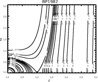
Figure 18.— Effective gravitational potential for magnetic field lines corotating with the Keplerian angular velocity (anchored in an accretion disk). Here, $r_{0}=1$. Shown are arbitrary equipotential surfaces, $\Phi(r,z)={\rm constant}$, chosen such that a cusp is seen at $r=r_{0}$ (Blandford & Payne, 1982).

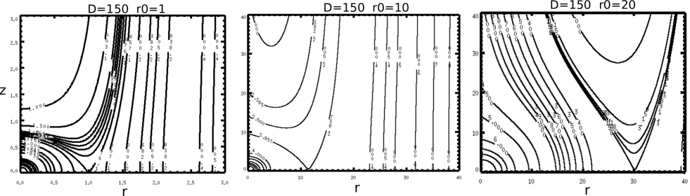
Figure 19.— Shown are the equipotential surfaces for beads on a wire co-rotating with the Keplerian velocity at $r_{0}$, and the whole system is part of the binary system. Different panel show the contours for different magnetic field footprint $r_{0}=1,10,20$ and binary separation $D=150$.

References

- Agudo et al. (2007) Agudo, I., Bach, U., Krichbaum, T. P., Marscher, A. P., Gonidakis, I., Diamond, P. J., Perucho, M., Alef, W., Graham, D. A., Witzel, A., Zensus, J. A., Bremer, M., Acosta-Pulido, J. A., & Barrena, R. 2007, A&A, 476, L17
- Artymowicz & Lubow (1994) Artymowicz, P. & Lubow, S. H. 1994, ApJ, 421, 651
- Bate et al. (2000) Bate, M. R., Bonnell, I. A., Clarke, C. J., Lubow, S. H., Ogilvie, G. I., Pringle, J. E., & Tout, C. A. 2000, MNRAS, 317, 773
- Beltrán et al. (2016) Beltrán, M. T., Cesaroni, R., Moscadelli, L., Sánchez-Monge, Á., Hirota, T., & Kumar, M. S. N. 2016, A&A, 593, A49
- Bisikalo et al. (2012) Bisikalo, D. V., Dodin, A. V., Kaigorodov, P. V., Lamzin, S. A., Malogolovets, E. V., & Fateeva, A. M. 2012, Astronomy Reports, 56, 686
- Blandford & Payne (1982) Blandford, R. D. & Payne, D. G. 1982, MNRAS, 199, 883
- Blondin (2000) Blondin, J. M. 2000, New Astronomy, 5, 53
- Bowen et al. (2017) Bowen, D. B., Campanelli, M., Krolik, J. H., Mewes, V., & Noble, S. C. 2017, ApJ, 838, 42
- Campbell et al. (1988) Campbell, B., Walker, G. A. H., & Yang, S. 1988, ApJ, 331, 902
- Casse & Keppens (2002) Casse, F. & Keppens, R. 2002, ApJ, 581, 988
- Cherepashchuk (2002) Cherepashchuk, A. 2002, Space Sci. Rev., 102, 23
- Cherepashchuk et al. (2013) Cherepashchuk, A. M., Sunyaev, R. A., Molkov, S. V., Antokhina, E. A., Postnov, K. A., & Bogomazov, A. I. 2013, MNRAS, 436, 2004
- Chiang & Murray-Clay (2004) Chiang, E. I. & Murray-Clay, R. A. 2004, ApJ, 607, 913
- Correia et al. (2008) Correia, A. C. M., Udry, S., Mayor, M., Eggenberger, A., Naef, D., Beuzit, J.-L., Perrier, C., Queloz, D., Sivan, J.-P., Pepe, F., Santos, N. C., & Ségransan, D. 2008, A&A, 479, 271
- Crocker et al. (2002) Crocker, M. M., Davis, R. J., Spencer, R. E., Eyres, S. P. S., Bode, M. F., & Skopal, A. 2002, MNRAS, 335, 1100
- Daemgen et al. (2013) Daemgen, S., Petr-Gotzens, M. G., Correia, S., Teixeira, P. S., Brandner, W., Kley, W., & Zinnecker, H. 2013, A&A, 554, A43
- Duchêne et al. (2002) Duchêne, G., Ghez, A. M., & McCabe, C. 2002, ApJ, 568, 771
- Durant et al. (2013) Durant, M., Kargaltsev, O., Pavlov, G. G., Kropotina, J., & Levenfish, K. 2013, ApJ, 763, 72
- Eisloffel et al. (1996) Eisloffel, J., Smith, M. D., Davis, C. J., & Ray, T. P. 1996, AJ, 112, 2086
- Fendt & Sheikhnezami (2013) Fendt, C. & Sheikhnezami, S. 2013, ApJ, 774, 12
- Fendt & Zinnecker (1998) Fendt, C. & Zinnecker, H. 1998, A&A, 334, 750
- Ferreira (1997) Ferreira, J. 1997, A&A, 319, 340
- Flock et al. (2011) Flock, M., Dzyurkevich, N., Klahr, H., Turner, N. J., & Henning, T. 2011, ApJ, 735, 122
- Fragner & Nelson (2010) Fragner, M. M. & Nelson, R. P. 2010, A&A, 511, A77
- Gravity Collaboration et al. (2017) Gravity Collaboration, Petrucci, P.-O., Waisberg, I., Le Bouquin, J.-B., Dexter, J., Dubus, G., Perraut, K., Kervella, P., Abuter, R., Amorim, A., Anugu, N., Berger, J. P., Blind, N., Bonnet, H., Brandner, W., Buron, A., Choquet, É., Clénet, Y., de Wit, W., Deen, C., Eckart, A., Eisenhauer, F., Finger, G., Garcia, P., Garcia Lopez, R., Gendron, E., Genzel, R., Gillessen, S., Gonte, F., Haubois, X., Haug, M., Haussmann, F., Henning, T., Hippler, S., Horrobin, M., Hubert, Z., Jochum, L., Jocou, L., Kok, Y., Kolb, J., Kulas, M., Lacour, S., Lazareff, B., Lèna, P., Lippa, M., Mérand, A., Müller, E., Ott, T., Panduro, J., Paumard, T., Perrin, G., Pfuhl, O., Ramos, J., Rau, C., Rohloff, R.-R., Rousset, G., Sanchez-Bermudez, J., Scheithauer, S., Schöller, M., Straubmeier, C., Sturm, E., Vincent, F., Wank, I., Wieprecht, E., Wiest, M., Wiezorrek, E., Wittkowski, M., Woillez, J., Yazici, S., & Zins, G. 2017, A&A, 602, L11
- Hawley et al. (2015) Hawley, J. F., Fendt, C., Hardcastle, M., Nokhrina, E., & Tchekhovskoy, A. 2015, Space Sci. Rev., 191, 441
- Herbst et al. (1996) Herbst, T. M., Beckwith, S. V. W., Glindemann, A., Tacconi-Garman, L. E., Kroker, H., & Krabbe, A. 1996, AJ, 111, 2403
- Hirth et al. (1997) Hirth, G. A., Mundt, R., & Solf, J. 1997, A&AS, 126, 437
- Jensen & Akeson (2014) Jensen, E. L. N. & Akeson, R. 2014, Nature, 511, 567
- Johnson et al. (2004) Johnson, J. A., Marcy, G. W., Hamilton, C. M., Herbst, W., & Johns-Krull, C. M. 2004, AJ, 128, 1265
- Johnson & Winn (2004) Johnson, J. A. & Winn, J. N. 2004, AJ, 127, 2344
- Johnston et al. (2003) Johnston, K. J., Gaume, R. A., Fey, A. L., de Vegt, C., & Claussen, M. J. 2003, AJ, 125, 858
- Ju et al. (2017) Ju, W., Stone, J. M., & Zhu, Z. 2017, ApJ, 841, 29
- Kley et al. (2008) Kley, W., Papaloizou, J. C. B., & Ogilvie, G. I. 2008, A&A, 487, 671
- Knigge & Livio (1998) Knigge, C. & Livio, M. 1998, MNRAS, 297, 1079
- Kraus et al. (2006) Kraus, S., Balega, Y., Elitzur, M., Hofmann, K.-H., Preibisch, T., Rosen, A., Schertl, D., Weigelt, G., & Young, E. T. 2006, A&A, 455, 521
- Lai (2014) Lai, D. 2014, MNRAS, 440, 3532
- Larwood et al. (1996) Larwood, J. D., Nelson, R. P., Papaloizou, J. C. B., & Terquem, C. 1996, MNRAS, 282, 597
- Lawler et al. (2010) Lawler, S. M., Herbst, W., Redfield, S., Hamilton, C. M., Johns-Krull, C. M., Winn, J. N., Johnson, J. A., & Mundt, R. 2010, ApJ, 711, 1297
- Lopez et al. (2006) Lopez, L. A., Marshall, H. L., Canizares, C. R., Schulz, N. S., & Kane, J. F. 2006, ApJ, 650, 338
- Luque-Escamilla et al. (2015) Luque-Escamilla, P. L., Martí, J., & Martínez-Aroza, J. 2015, A&A, 584, A122
- Margon & Anderson (1989) Margon, B. & Anderson, S. F. 1989, ApJ, 347, 448
- Margon et al. (1979) Margon, B., Grandi, S. A., Stone, R. P. S., & Ford, H. C. 1979, ApJ, 233, L63
- Marshall et al. (2013) Marshall, H. L., Canizares, C. R., Hillwig, T., Mioduszewski, A., Rupen, M., Schulz, N. S., Nowak, M., & Heinz, S. 2013, ApJ, 775, 75
- Mignone et al. (2007) Mignone, A., Bodo, G., Massaglia, S., Matsakos, T., Tesileanu, O., Zanni, C., & Ferrari, A. 2007, ApJS, 170, 228
- Mignone et al. (2013) Mignone, A., Striani, E., Tavani, M., & Ferrari, A. 2013, MNRAS, 436, 1102
- Mignone et al. (2012) Mignone, A., Zanni, C., Tzeferacos, P., van Straalen, B., Colella, P., & Bodo, G. 2012, ApJS, 198, 7
- Mioduszewski et al. (2004) Mioduszewski, A. J., Rupen, M. P., Walker, R. C., Schillemat, K. M., & Taylor, G. B. 2004, in Bulletin of the American Astronomical Society, Vol. 36, AAS/High Energy Astrophysics Division #8, 967
- Mirabel & Rodríguez (1999) Mirabel, I. F. & Rodríguez, L. F. 1999, ARA&A, 37, 409
- Miranda & Lai (2015) Miranda, R. & Lai, D. 2015, MNRAS, 452, 2396
- Monceau-Baroux et al. (2015) Monceau-Baroux, R., Porth, O., Meliani, Z., & Keppens, R. 2015, A&A, 574, A143
- Müller & Kley (2012) Müller, T. W. A. & Kley, W. 2012, A&A, 539, A18
- Mundt et al. (2010) Mundt, R., Hamilton, C. M., Herbst, W., Johns-Krull, C. M., & Winn, J. N. 2010, ApJ, 708, L5
- Murphy et al. (2010) Murphy, G. C., Ferreira, J., & Zanni, C. 2010, A&A, 512, A82+
- Murray & Chiang (1996) Murray, N. & Chiang, J. 1996, Nature, 382, 789
- Nixon et al. (2013) Nixon, C., King, A., & Price, D. 2013, MNRAS, 434, 1946
- Owen & Lai (2017) Owen, J. E. & Lai, D. 2017, MNRAS, 469, 2834
- Paczynski (1977) Paczynski, B. 1977, ApJ, 216, 822
- Papaloizou et al. (1997) Papaloizou, J. C. B., Larwood, J. D., Nelson, R. P., & Terquem, C. 1997, in Lecture Notes in Physics, Berlin Springer Verlag, Vol. 487, Accretion Disks - New Aspects, ed. E. Meyer-Hofmeister & H. Spruit, 182
- Papaloizou & Pringle (1977) Papaloizou, J. C. B. & Pringle, J. E. 1977, MNRAS, 181, 441
- Papaloizou & Pringle (1983) —. 1983, MNRAS, 202, 1181
- Papaloizou & Terquem (1995) Papaloizou, J. C. B. & Terquem, C. 1995, MNRAS, 274, 987
- Paron et al. (2016) Paron, S., Fariña, C., & Ortega, M. E. 2016, A&A, 593, A132
- Pelletier & Pudritz (1992) Pelletier, G. & Pudritz, R. E. 1992, ApJ, 394, 117
- Pichardo et al. (2005) Pichardo, B., Sparke, L. S., & Aguilar, L. A. 2005, MNRAS, 359, 521
- Picogna & Marzari (2015) Picogna, G. & Marzari, F. 2015, A&A, 583, A133
- Pudritz & Norman (1983) Pudritz, R. E. & Norman, C. A. 1983, ApJ, 274, 677
- Pudritz et al. (2007) Pudritz, R. E., Ouyed, R., Fendt, C., & Brandenburg, A. 2007, Protostars and Planets V, 277
- Queloz et al. (2000) Queloz, D., Mayor, M., Weber, L., Blécha, A., Burnet, M., Confino, B., Naef, D., Pepe, F., Santos, N., & Udry, S. 2000, A&A, 354, 99
- Raga et al. (2009) Raga, A. C., Esquivel, A., Velázquez, P. F., Cantó, J., Haro-Corzo, S., Riera, A., & Rodríguez-González, A. 2009, ApJ, 707, L6
- Seifina & Titarchuk (2010) Seifina, E. & Titarchuk, L. 2010, ApJ, 722, 586
- Sheikhnezami & Fendt (2015) Sheikhnezami, S. & Fendt, C. 2015, ApJ, 814, 113
- Sheikhnezami et al. (2012) Sheikhnezami, S., Fendt, C., Porth, O., Vaidya, B., & Ghanbari, J. 2012, ApJ, 757, 65
- Shepherd et al. (2000) Shepherd, D. S., Yu, K. C., Bally, J., & Testi, L. 2000, ApJ, 535, 833
- Shi et al. (2012) Shi, J.-M., Krolik, J. H., Lubow, S. H., & Hawley, J. F. 2012, ApJ, 749, 118
- Silber et al. (1994) Silber, A. D., Remillard, R. A., Horne, K., & Bradt, H. V. 1994, ApJ, 424, 955
- Smith et al. (2002) Smith, D. M., Heindl, W. A., & Swank, J. H. 2002, ApJ, 569, 362
- Soker & Lasota (2004) Soker, N. & Lasota, J.-P. 2004, A&A, 422, 1039
- Stepanovs & Fendt (2014) Stepanovs, D. & Fendt, C. 2014, ApJ, 793, 31
- Stepanovs & Fendt (2016) —. 2016, ApJ, 825, 14
- Stepanovs et al. (2014) Stepanovs, D., Fendt, C., & Sheikhnezami, S. 2014, ApJ, 796, 29
- Suzuki & Inutsuka (2014) Suzuki, T. K. & Inutsuka, S.-i. 2014, ApJ, 784, 121
- Terquem et al. (1999) Terquem, C., Eislöffel, J., Papaloizou, J. C. B., & Nelson, R. P. 1999, ApJ, 512, L131
- Truss (2007) Truss, M. R. 2007, MNRAS, 376, 89
- Velázquez et al. (2013) Velázquez, P. F., Raga, A. C., Cantó, J., Schneiter, E. M., & Riera, A. 2013, MNRAS, 428, 1587
- Vlemmings et al. (2006) Vlemmings, W. H. T., Diamond, P. J., & Imai, H. 2006, Nature, 440, 58
- von Rekowski et al. (2003) von Rekowski, B., Brandenburg, A., Dobler, W., Dobler, W., & Shukurov, A. 2003, A&A, 398, 825
- Wang et al. (2017) Wang, S., Bai, Y., Zhang, C.-P., & Liu, J.-F. 2017, Research in Astronomy and Astrophysics, 17, 10
- Winn et al. (2004) Winn, J. N., Holman, M. J., Johnson, J. A., Stanek, K. Z., & Garnavich, P. M. 2004, ApJ, 603, L45
- Zanni et al. (2007) Zanni, C., Ferrari, A., Rosner, R., Bodo, G., & Massaglia, S. 2007, A&A, 469, 811
- Zhu & Stone (2017) Zhu, Z. & Stone, J. M. 2017, ArXiv e-prints