Optimal parametrizations of a class of self-affine sets

Abstract.

In this paper, we study optimal parametrizations of the invariant sets of a single matrix graph IFS which is a generalization of [12].We show that the invariant sets of a linear single matrix GIFS which has primitive associated matrix and satisfies the open set condition admit optimal parametrizations. This result is the basis of further study of space-filling curves of self-affine sets.

1. Introduction

The topic of space-filling curves has a very long history. Recently, Rao and Zhang [12] as well as Dai, Rao, and Zhang [4] found a systematic method to construct space-filling curves for connected self-similar sets satisfying the open set condition. This method generalizes almost all known results in this field.

The self-affine sets have more complex structures than self-similar due to the different contraction ratios in different directions. There are almost no systematic works on the space-filling curves of self-affine sets except some examples provided by Dekking [5], Sirvent’s study under some special conditions [13, 14], boundary parametrizations of self-affine tiles by Akiyama and Loridant [1, 2], and boundary parametrizations of a class of cubic Rauzy fractals by Loridant [10]. The purpose of the present paper is to carry out studies in this direction. In particular, we study the space-filling curves (or optimal parameterizations) of single-matrix graph-directed systems.

1.1. Single-matrix GIFS

Let $(\mathcal{A},\Gamma)$ be a directed graph with vertex set $\mathcal{A}$ and edge set $\Gamma$. Let

$$\mathcal{G}=\{g_{e}:\mathbb{R}^{d}\rightarrow\mathbb{R}^{d};~{}e\in\Gamma\}$$

be a collection of contractions. The triple $(V,\Gamma,\mathcal{G})$, or simply $\mathcal{G}$, is called a graph-directed iterated function system (GIFS). Usually, we set $\mathcal{A}=\{1,2,\dots,N\}$. Let $\Gamma_{ij}$ be the set of edges from vertex $i$ to $j$, then there exist unique non-empty compact sets $\{E_{i}\}_{i=1}^{N}$ satisfying

(1.1) $$E_{i}=\bigcup_{j=1}^{N}\bigcup_{e\in\Gamma_{ij}}g_{e}(E_{j}),\quad\quad 1\leq i\leq N.$$

The family $\{E_{i}\}_{i=1}^{N}$ is called the family of invariant sets of the GIFS (cf. [11]). When the graph has only one vertex with self-edges, then the GIFS will degenerate into an iterated function system (IFS).

We say that the system $\mathcal{G}$ satisfies the open set condition (OSC) if there exist non-empty open sets $U_{1},\dots,U_{N}$ such that

$$U_{i}\subset\bigcup_{j=1}^{N}\bigcup_{e\in\Gamma_{ij}}g_{e}(U_{j}),\quad\quad 1\leq i\leq N,$$

and the right hand sets union are disjoint.

Denote $M=(m_{ij})_{1\leq i,j\leq N}$ the associated matrix of the directed graph $(\mathcal{A},\Gamma)$, that is, $m_{ij}=\sharp\Gamma_{ji}$ counts the number of edges from $j$ to $i$. We say a directed graph $({\mathcal{A}},\Gamma)$ is primitive, if the associated matrix is primitive, i.e., $M^{n}$ is a positive matrix for some $n$. (See [11], [6].) In this paper, we always assume that $({\mathcal{A}},\Gamma)$ is primitive.

According to Luo and Yang [8], ${\mathcal{G}}$ is called a single-matrix GIFS if there is a $d\times d$ expanding matrix $A$ such that all functions related to $e\in\Gamma$ have the form

(1.2) $$g_{e}(x)=A^{-1}(x+d_{e}),$$

where $d_{e}\in\mathbb{R}^{d}$.

1.2. Optimal parametrization

Let $E\subset\mathbb{R}^{d}$ be a compact set and ${\mathcal{H}}^{s}(E)$ denote the Hausdorff measure with respect to Euclidean norm of $E$. Basically, if $\psi:[0,1]\to E$ is a continuous onto mapping, then $\psi$ is a parametrization of $E$. If $E$ is a self-similar set satisfying the open set condition, then $0<{\mathcal{H}}^{s}(E)<\infty$, where $s$ is the Hausdorff dimension of $E$. In this case, we may expect that $E$ has a better parametrization. The following concept is first given by Dai and Wang [3]:

Definition 1.1.

A surjective mapping $\psi:[0,1]\rightarrow E$ is called an optimal parametrization of $E$ if the following conditions are fulfilled.

1. $\psi$ is a measure isomorphism between $([0,1],$${\mathcal{B}}([0,1]),$${\mathcal{L}})$ and $(E,{\mathcal{B}}(E),{\mathcal{H}}^{s})$, that is, there exist $E^{\prime}\subset E$ and $I^{\prime}\subset[0,1]$ with full measure such that $\psi:~{}I^{\prime}\to E^{\prime}$ is a bijection and it is measure-preserving in the sense that

   $${\mathcal{H}}^{s}(\psi(F))=c{\mathcal{L}}(F)\text{ and }{\mathcal{L}}(\psi^{-1}(B))=c^{-1}{\mathcal{H}}^{s}(B),$$

   for any Borel set $F\subset[0,1]$ and any Borel set $B\subset E$, where $c={\mathcal{H}}^{s}(E)$. (See for instance, Walters [15].)

2. $\psi$ is $1/s$-Hölder continuous, that is, there is a constant $c^{\prime}>0$ such that

   $$\|\psi(x)-\psi(y)\|\leq c^{\prime}\|x-y\|^{\frac{1}{s}}\ \text{ for all }x,y\in[0,1].$$

   We call $1/s$ the Hölder exponent.

For a self-affine set $K$, the Hausdorff measure may be $0$ or $\infty$, and hence we cannot require an optimal parametrization satisfying (i) of the above. Also, the $1/s$-Hölder continuity may fail. So we are forced to define the optimal parametrization in some other way.

To this end, we choose a pseudo-norm $\|\cdot\|_{\omega}$ instead of the Euclidean norm on $K$. This pseudo-norm is first introduced by Lemarié-Rieusset [9] to deal with problems in the theory of wavelets. He and Lau [7] developed the Hausdorff dimension (denoted by $\text{dim}_{\omega}$) and Hausdorff measure (denoted by $\mathcal{H}_{\omega}^{s}$) with respect to pseudo-norm (see Section 2 for details). The advantage of the pseudo-norm is that we can regard the expanding matrix $A$ as a ‘similitude’. By replacing the norm, dimension and measure by their counterpart w.r.t.the pseudo-norm, we can define an optimal parametrization similar to Definition 1.1; details will be given in Section 2.

1.3. Linear GIFS and our main result

We equip a GIFS with an order structure (and call it an ordered GIFS), which induces a lexicographical order of the associated symbolic space. An ordered GIFS is called a linear GIFS if every two consecutive cylinders have nonempty intersections (see section 2 for precise definitions).

Rao and Zhang [12] proved that as soon as we find a linear GIFS structure of a self-similar set, then a space-filling curve can be constructed accordingly. Dai, Rao, and Zhang [4] develop a very general method to explore linear GIFS structures of a given self-similar set. In this paper, we only deal with the first problem for self-affine sets. Our main result is

Theorem 1.2.

Let $(\mathcal{A},\Gamma,\mathcal{G},\prec)$ be a linear single-matrix graph-directed IFS with expanding matrix $A$ satisfying the open set condition and assume that the associated matrix $M$ of the graph is primitive. Then there exists a parametrization $\psi_{j}$ of the invariant $E_{j}$ for all $j\in\mathcal{A}$ such that

1. $\psi_{j}$ is a measure isomorphism between

   $$([0,1],{\mathcal{B}}([0,1]),{\mathcal{L}})\text{ and }(E_{j},{\mathcal{B}}(E_{j}),{\mathcal{H}}_{\omega}^{s}).$$

2. There is a constant $c>0$ such that

   $$\|\psi_{j}(x)-\psi_{j}(y)\|_{\omega}\leq c\|x-y\|^{\frac{1}{\alpha}}\ \text{ for all }x,y\in[0,1],$$

   where $\alpha=\dim_{\omega}E_{j}$.

According to the relation between Euclidean norm and pseudo-norm, we have the following result for the Hölder continuity of the parametrization $\psi_{j}$ obtained by the above theorem.

Corollary 1.3.

Let $\lambda_{M}$ be the maximal eigenvalue of $M$. Let $\lambda_{max}$ and $\lambda_{min}$ be the maximal modulus and minimal modulus of the eigenvalues of $A$, respectively. For any $0<\epsilon<\lambda_{min}-1$,

We will close this section by three examples, where the substitution rules induced linear GIFS are given directly. We shall discuss in subsequent paper on how to obtain substitution rules, and once we have a substitution rule, the GIFS is constructed automatically. In the following examples, we calculate the value of Hölder exponent and it will be interesting to compare this with the value obtained from Corollary 1.3.

• $\psi_{j}$ is $\frac{\ln(\lambda_{\max}+\epsilon)}{\ln\lambda_{M}}$-Hölder continuous if $\|\psi_{j}(x)-\psi_{j}(y)\|\geq 1$;

• $\psi_{j}$ is $\frac{\ln(\lambda_{\min}-\epsilon)}{\ln\lambda_{M}}$-Hölder continuous if $\|\psi_{j}(x)-\psi_{j}(y)\|\leq 1$.

The matrices $M$ and $A$ have the same meaning as in the above theorem.

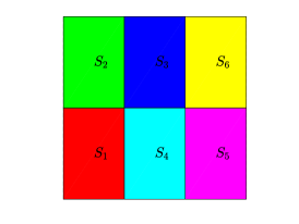
(a) Unit square $Q=\cup_{i=1}^{6}S_{i}(Q)$.

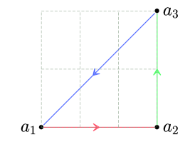
(b) Initial cycle.

(c) First generation.

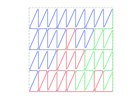
(d) Second generation.

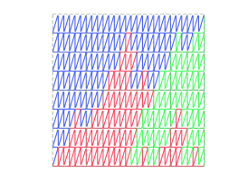
(e) Third generation.

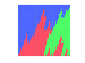
(f) Parametrized square.

Figure 1. The space-filling curve of unit square given by IFS $\{S_{i}\}_{i=1}^{6}$.

In the following examples, we always use ${\bf e}_{1},{\bf e}_{2}$ to denote the standard basis of $\mathbb{R}^{2}$. Denote the maximal eigenvalue of $M$ by $\lambda_{M}$. And denote by the Hölder exponent with respect to Euclidean norm Hölder_E.

Example 1.

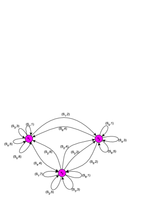
Figure 2. The directed graph $G$ with vertex set $\{v_{1},v_{2},v_{3}\}$ and labelled edges obtained by the substitution rule (1.3). The label $(S,i)$ with $S\in\{S_{i}\}_{i=1}^{6}$ and $i\in\mathbb{N}$ means that $S$ is the contraction for the $i$-th edge starting from this vertex. The graph here determins a GIFS.

A unit square. Let $Q$ be the unit square generated by the IFS $S_{i}(x)=A^{-1}(x+d_{i}),~{}~{}d_{i}\in\mathcal{D}$, where $\mathcal{D}=\{0,{\bf e}_{2},{\bf e}_{1}+{\bf e}_{2},{\bf e}_{1},2{\bf e}_{1},2{\bf e}_{1}+{\bf e}_{2}\}$, and the expanding matrix is $A=\left(\begin{matrix}3&0\\ 0&2\\ \end{matrix}\right)$. Let $a_{1},a_{2},a_{3}$ be the three vertice of the unit square, see Figure 1(b). Denote by $v_{i}$ the edge from $a_{i}$ to $a_{i+1},i=1,2,3$ (assume $a_{4}=a_{1}$). By the similar idea as Dai, Rao, and Zhang [4], we can construct the following substitution rule which means to replace an edge $v_{i}$ by a trail which shares the same starting point and ending point with $v_{i}$.

(1.3) $$\begin{split}v_{1}\longrightarrow\vphantom{a}&S_{1}(v_{1})+S_{1}(v_{2})+S_{3}(v_{1})+S_{4}(v_{3})+S_{4}(v_{1})+S_{5}(v_{1}),\\ v_{2}\longrightarrow\vphantom{a}&S_{5}(v_{2})+S_{5}(v_{3})+S_{4}(v_{2})+S_{6}(v_{1})+S_{6}(v_{2}),\\ v_{3}\longrightarrow\vphantom{a}&S_{6}(v_{3})+S_{3}(v_{2})+S_{3}(v_{3})+S_{2}(v_{2})+S_{2}(v_{3})+S_{2}(v_{1})+S_{1}(v_{3}),\end{split}$$

where we use the symbol ${}^{\prime}+^{\prime}$ to connect the consecutive edges or sub-trails. It is shown in [4] that the above substitution rule induces a GIFS (see Figure 2) which is linear. We will show the set equation form of the GIFS in Section 3. The associated matrix of the substitution which is defined as the associated matrix of the directed graph $G$ obtained by the substitution is

$$M=\left(\begin{matrix}4&1&1\\ 1&3&2\\ 1&1&4\\ \end{matrix}\right),\quad\lambda_{M}=6,\quad\text{H\"{o}lder}_{E}=\log_{6}2.$$

Compared with the unit square parametrized using the method as Hilbert or Peano which have the Hölder exponent $\frac{1}{2}$, the parametrization obtained here doesn’t have a better smoothness.

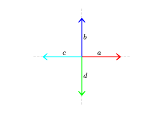
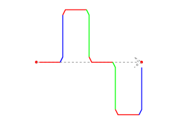
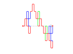
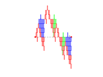
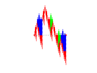
Figure 3. The figures show the first four approximation of $E_{1}$.

Example 2.

Dekking’s plane filling curve [5]. It is induced by the following substitution:

$$\begin{matrix}\sigma:&a\mapsto abadadab;\quad b\mapsto cbcbadab;\quad c\mapsto cbcbcdadcbcd;\quad d\mapsto adcd.\end{matrix}$$

The set equation form of this substitution can be found in Section 3 and we obtain a linear GIFS as well. In this example, the expanding matrix is $A=\left(\begin{matrix}4&0\\ 0&2\\ \end{matrix}\right)$ and associated matrix of the substitution is

$$M=\left(\begin{matrix}4&2&1&1\\ 2&3&3&0\\ 0&2&5&1\\ 2&1&3&2\\ \end{matrix}\right),\quad\lambda_{M}=8,\quad\text{H\"{o}lder}_{E}=\frac{1}{3}.$$

Then we can check that Hölder_E is between the two Hölder exponents obtained by Corollary 1.3.

Example 3.

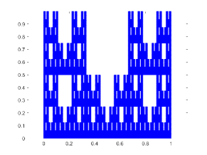
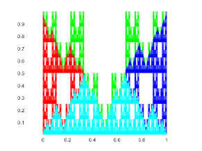
Figure 4. The left is Mcmullen set $T$ and the right is $\cup_{i=1}^{5}E_{i}$.

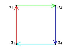
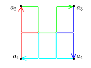
Figure 5. Substitution rule of the Mcmullen set

A McMullen set. We consider the McMullen set depicted in Figure  4, left. Denote the four vertices of the unit square by $a_{1},a_{2},a_{3},a_{4}$. Denote $v_{i}=\overrightarrow{a_{i}a_{i+1}},i=1,2,3,4~{}(\text{ assume }a_{5}=a_{1}),$ and we get the following substitution rule (which is obtained from replacing the edge from $a_{i}$ to $a_{i+1}$ (left, Figure 5) by the trail from $a_{i}$ to $a_{i+1}$ (right, Figure 5)).

$$v_{1}\longrightarrow\vphantom{a} S_{1}(v_{1})+S_{1}(v_{2})+S_{4}(v_{4})+S_{4}(v_{1}),$$

$$v_{2}\longrightarrow\vphantom{a} S_{4}(v_{2})+S_{4}(v_{3})+S_{2}(v_{2})+S_{5}(v_{1})+S_{5}(v_{2}),$$

$$v_{3}\longrightarrow\vphantom{a} S_{5}(v_{3})+S_{5}(v_{4})+S_{3}(v_{2})+S_{3}(v_{3}),$$

$$v_{4}\longrightarrow\vphantom{a} S_{3}(v_{4})+S_{3}(v_{1})+S_{2}(v_{3})+S_{2}(v_{4})+S_{2}(v_{1})+S_{1}(v_{3})+S_{1}(v_{4}).$$

In this example, the expanding matrix is $A=\left(\begin{matrix}3&0\\ 0&2\\ \end{matrix}\right)$ and the associated matrix of the substitution is

$$M=\left(\begin{matrix}2&1&0&2\\ 1&3&1&0\\ 0&1&2&2\\ 1&0&1&3\\ \end{matrix}\right),\quad\lambda_{M}=5,\quad\text{H\"{o}lder}_{E}=\log_{5}2.$$

Figure 6 shows the visualization of the filling curve of the Mcmullen set $T$. To give a self-avoiding visualization, we round off the corners of the approximating curves.

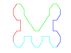
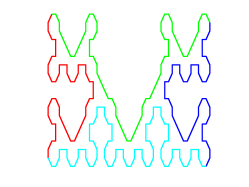
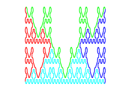
Figure 6. The first three approximations to the filling curve of Mcmullen set of Example 3.

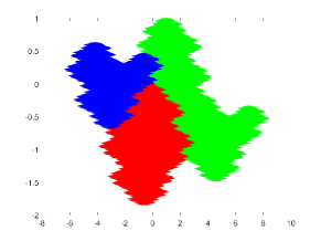
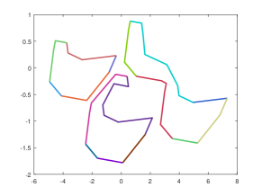
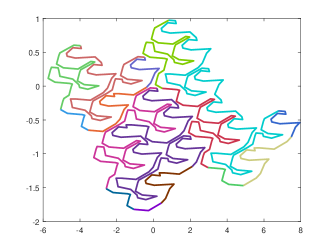
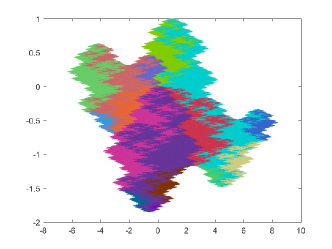
Figure 10. The first figure is the Rauzy fractal given by the substition $\sigma:1\longrightarrow 12321,2\longrightarrow 321,3\longrightarrow 2$. The following three Figures show the first three approximations of the filling curve of this Rauzy fractal.

Inspired by [4], we shall do some further study on space-filling curve of self-affine fractals, such as space-filling curves of McMullen sets and of Rauzy fractals. To this matter, we try to find a similar method as we did for self-similar sets to construct a linear GIFS from a self-affine set or from a Rauzy fractal (See Figure 10 where we shows the approximations of the filling curve of a Rauzy fractal). Here we want to emphasis that to do the parametrization of a Rauzy fractal is based on invariant sets of a graph-directed iterated system, that is to say, we construct a linear GIFS from a given GIFS. ([4] focused on constructing a linear GIFS from a given IFS.) However, to construct a linear GIFS from the original iterated function system or from graph-directed iterated function system is a complicated work, so we will not do the part of constructions of linear GIFS and only give the set equations of linear GIFS in present paper. Hopefully, it will be shown in our following work. Figure 10 shows an interesting example of Rauzy fractal.

This paper is organised in the following way. In Section 2, we recall some definitions and notations, and then we give some additional explanations of the Examples  1, 2, and 3 in Section 3. The last section is devoted to the verification of our main Theorem 1.2.

2. Preliminaries

2.1. The symbolic space related to a graph $G$

Let $G=(\mathcal{A},\Gamma)$ be a directed graph. A sequence of edges in $G$, denoted by ${\boldsymbol{\omega}}=\omega_{1}+\omega_{2}+\dots+\omega_{n}$, is called a walk, if the terminal state of $\omega_{i}$ coincides with the initial state of $\omega_{i+1}$ for $1\leq i\leq n-1$. A walk is called a trail, if all the edges appearing in the walk are distinct. A trail is called a path if all the vertices are distinct. For $i\in\mathcal{A}$, let

$$\Gamma_{i}^{k},\ \Gamma_{i}^{\ast},\text{ and }\Gamma_{i}^{\infty}$$

be the set of all walks of length $k$, the set of all walks of finite length, and the set of all infinite walks, starting at state $i$, respectively. Note that $\Gamma_{i}^{\ast}=\bigcup_{k\geq 1}\Gamma_{i}^{k}$.

For ${\boldsymbol{\omega}}=(\omega_{k})_{k=1}^{\infty}$, define by ${\boldsymbol{\omega}}|_{n}=\omega_{1}+\omega_{2}+\dots+\omega_{n}$ the prefix of ${\boldsymbol{\omega}}$ of length $n$. Moreover, call $[\omega_{1}\dots\omega_{n}]:=\{{\boldsymbol{\gamma}}\in\Gamma_{i}^{\infty};~{}~{}{\boldsymbol{\gamma}}|_{n}=\omega_{1}+\dots+\omega_{n}\}$ the cylinder associated with a walk $\omega_{1}+\dots+\omega_{n}$.

For a walk ${\boldsymbol{\gamma}}=\gamma_{1}+\dots+\gamma_{n}\in\Gamma_{i}^{n}$, set $g_{{\boldsymbol{\gamma}}}:=g_{\gamma_{1}}\circ g_{\gamma_{2}}\dots\circ g_{\gamma_{n}}$, then we denote

$$E_{\boldsymbol{\gamma}}:=g_{{\boldsymbol{\gamma}}}(E_{t({\boldsymbol{\gamma}})}),$$

where $t({\boldsymbol{\gamma}})$ denotes the terminal state of the path $\boldsymbol{\gamma}$ (which equals$\gamma_{n}$ here). Iterating (1.1) $k$-times, we obtain

(2.1) $$E_{i}=\bigcup_{{\boldsymbol{\gamma}}\in\Gamma_{i}^{k}}E_{\boldsymbol{\gamma}}.$$

We define the projection $\pi:\Gamma_{1}^{\infty}\times\dots\times\Gamma_{N}^{\infty}\rightarrow\mathbb{R}^{d}\times\dots\times\mathbb{R}^{d}$, where $\pi_{i}:\Gamma_{i}^{\infty}\rightarrow\mathbb{R}^{d}$ is given by

(2.2) $$\{\pi_{i}({\boldsymbol{\omega}})\}:=\bigcap_{n\geq 1}E_{\boldsymbol{\omega|_{n}}}.$$

For $x\in E_{i}$, we call ${\boldsymbol{\omega}}$ a coding of $x$ if $\pi_{i}({\boldsymbol{\omega}})=x$. It is easy to see that $\pi_{i}(\Gamma_{i}^{\infty})=E_{i}$.

2.2. Pseudo-norm and Hausdorff measure in pseudo-norm

Denote by $B(x,r)$ the open ball with center $x$ and radius $r$. Recall that $A$ is the expanding matrix with $|\det A|=q$, then $V=A(B(0,1))\setminus B(0,1)$ is homeomorphic to an annulus. For $\delta\in(0,\frac{1}{2})$, choose a positive $\mathbb{C}^{\infty}$-function $\phi_{\delta}(x)$ with support in $B(0,\delta)$ such that $\phi_{\delta}(x)=\phi_{\delta}(-x)$ and $\int\phi_{\delta}(x)dx=1$, and then define a pseudo-norm $\|\cdot\|_{\omega}$ in $\mathbb{R}^{d}$ by

$$\|x\|_{\omega}=\sum_{n\in\mathbb{Z}}q^{-n/d}h(A^{n}x),$$

where $h(x)=\chi_{V}*\phi_{\delta}(x)=\int_{\mathbb{R}^{d}}\chi_{V}(x-y)\cdot\phi_{\delta}(y)dy$.

We list some basic properties of $\|\cdot\|_{\omega}$.

Proposition 2.1.

(See [7, Proposition 2.1]) The function $\|\cdot\|_{\omega}$ satisfies the following conditions.

(i) $\|x\|_{\omega}\geq 0$; $\|x\|_{\omega}=0$ if and only if $x=0$.

(ii) $\|x\|_{\omega}=\|-x\|_{\omega}$;

(iii) $\|Ax\|_{\omega}=q^{1/d}\|x\|_{\omega}\geq\|x\|_{\omega}$ for all $x\in\mathbb{R}^{d}$.

(iv) There exists a constant $\beta>0$ such that $\|x+y\|_{\omega}\leq\beta\max\{\|x\|_{\omega},\|y\|_{\omega}\}$ for any $x,y\in\mathbb{R}^{d}$.

The pseudo-norm $\|\cdot\|_{\omega}$ is comparable with the Euclidean norm $\|x\|$ .

Proposition 2.2.

(See [7, Proposition 2.4]) Let $\lambda_{\max}$ and $\lambda_{\min}$ be the maximal modulus and minimal modulus of the eigenvalues of $A$, respectively. For any $0<\varepsilon<\lambda_{\min}-1$, there exists $C>0$(depends on $\varepsilon$) such that

$$C^{-1}\|x\|^{\ln q/d\ln(\lambda_{\max}+\varepsilon)}\leq\|x\|_{\omega}\leq C\|x\|^{\ln q/d\ln(\lambda_{\min}-\varepsilon)},\quad\text{ if }\|x\|>1;$$

$$C^{-1}\|x\|^{\ln q/d\ln(\lambda_{\min}-\varepsilon)}\leq\|x\|_{\omega}\leq C\|x\|^{\ln q/d\ln(\lambda_{\max}+\varepsilon)},\quad\text{ if }\|x\|\leq 1.$$

The Hausdorff measure with respect to the pseudo-norm $\|\cdot\|_{\omega}$ was given by He and Lau [7] as follows. For $E\subset\mathbb{R}^{d}$, set $\text{diam}_{\omega}E=\text{sup}\{\|x-y\|_{\omega};~{}~{}x,y\in E\}$ to be the $\omega$-diameter of $E$. For $s\geq 0,\delta>0$, set

$$\mathcal{H}_{\omega,\delta}^{s}(E)=\inf\big{\{}\sum_{i=1}^{\infty}(\text{diam}_{\omega}E_{i})^{s};~{}~{}E\subset\bigcup_{i}E_{i},~{}~{}\text{diam}_{\omega}E_{i}\leq\delta\big{\}},$$

$$\mathcal{H}_{\omega}^{s}(E)=\lim_{\delta\rightarrow 0}\mathcal{H}_{\omega,\delta}^{s}(E).$$

$\mathcal{H}_{\omega}^{s}$ has the translation invariance property and the scaling property [7], that is,

$$\mathcal{H}_{\omega}^{s}(E+x)=\mathcal{H}_{\omega}^{s}(E)\text{ and }\mathcal{H}_{\omega}^{s}(A^{-1}E)=q^{-s/d}\mathcal{H}_{\omega}^{s}(E).$$

Thus the Hausdorff dimension with respect to $\|\cdot\|_{\omega}$ can be defined by

$$\dim_{\omega}E=\inf\{s;~{}~{}\mathcal{H}_{\omega}^{s}(E)=0\}=\sup\{s;~{}~{}\mathcal{H}_{\omega}^{s}(E)=\infty\}.$$

2.3. Linear GIFS

Let $({\mathcal{A}},\Gamma,\mathcal{G})$ be a GIFS with vertex set $\mathcal{A}$, edge set $\Gamma$ and mapping set $\mathcal{G}$. Let $\Gamma_{i}=\Gamma_{i}^{1}$ be the set of outgoing edges from the state $i$. We call $({\mathcal{A}},\Gamma,\mathcal{G},\prec)$ an ordered GIFS, if $\prec$ is a partial order on $\Gamma$ such that

1. $\prec$ is a linear order when restricted on $\Gamma_{j}$ for every $j\in{\mathcal{A}}$;

2. elements in $\Gamma_{i}\text{ and }\Gamma_{j}$ are not comparable if $i\neq j$.

(See [12] for detail.)

The order $\prec$ induces a lexicographical order on each $\Gamma_{i}^{k}$. Observe that $(\Gamma_{i}^{k},\prec)$ is a linear order; two paths ${\boldsymbol{\gamma}},{\boldsymbol{\omega}}\in\Gamma_{i}^{k}$ are said to be adjacent if there is no walk between them with respect to the order $\prec$.

Definition 2.3.

(see [12]) An ordered GIFS $({\mathcal{A}},\Gamma,\mathcal{G},\prec)$ with invariant sets $\{E_{i}\}_{i=1}^{N}$ is called a linear GIFS, if for all $i\in{\mathcal{A}}$ and $k\geq 1$,

$$E_{\boldsymbol{\gamma}}\cap E_{\boldsymbol{\omega}}\neq\emptyset$$

for adjacent walks ${\boldsymbol{\gamma}},{\boldsymbol{\omega}}$ in $\Gamma_{i}^{k}$ .

For $i\in\mathcal{A}$, a walk ${\boldsymbol{\omega}}\in\Gamma_{i}^{\infty}$ is called the lowest walk, if ${\boldsymbol{\omega}}|_{n}$ is the lowest walk in $\Gamma_{i}^{n}$ for all $n$; in this case, we call $a=\pi_{i}({\boldsymbol{\omega}})$ the head of $E_{i}$. Similarly, we define the highest walk ${\boldsymbol{\omega}}^{\prime}$ of $\Gamma_{i}^{\infty}$, and we call $b=\pi_{i}({\boldsymbol{\omega}}^{\prime})$ the the tail of $E_{i}$.

Definition 2.4.

(see [12, Definition 4.1] )An ordered GIFS is said to satisfy the chain condition, if for any $i\in{\mathcal{A}}$, and any two adjacent edges $\omega,\gamma\in\Gamma_{i}$ with $\omega\prec\gamma$,

$$g_{\omega}(\text{tail of }E_{t(\omega)})=g_{\gamma}(\text{ head of }E_{t(\gamma)}).$$

Lemma 2.5.

An ordered GIFS is a linear GIFS if and only if it satisfies the chain condition.

Remark. Definition 2.3, Definition 2.4 and Lemma 2.5 still make sense when $({\mathcal{A}},\Gamma,\mathcal{G})$ is a single matrix GIFS.

3. Examples

In this section, we will give the set equation form of substitution rules which we showed in the previous examples and explain simply that these induced GIFS are linear.

Example 4.

A unit square. Through the edge-to-trail substitution rule, we get the following GIFS in the set equation form.

$$E_{1}\circeq\vphantom{a} S_{1}(E_{1})\cup S_{1}(E_{2})\cup S_{3}(E_{1})\cup S_{4}(E_{3})\cup S_{4}(E_{1})\cup S_{5}(E_{1}),$$

$$E_{2}\circeq\vphantom{a} S_{5}(E_{2})\cup S_{5}(E_{3})\cup S_{4}(E_{2})\cup S_{6}(E_{1})\cup S_{6}(E_{2}),$$

$$E_{3}\circeq\vphantom{a} S_{6}(E_{3})\cup S_{3}(E_{2})\cup S_{3}(E_{3})\cup S_{2}(E_{2})\cup S_{2}(E_{3})\cup S_{2}(E_{1})\cup S_{1}(E_{3}).$$

Here we use $``\circeq"$ to emphasize that it is an ordered GIFS. By the result of [4], the above induced GIFS is a linear GIFS, or we can check it by Lemma 2.4 directly.

Example 5.

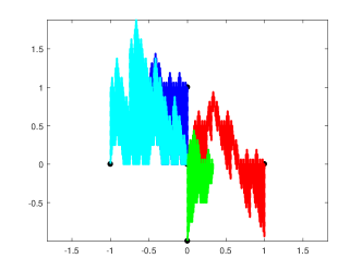
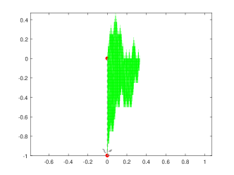
Figure 7. The left figure is $E=\cup_{i=1}^{4}E_{i}$, and the right one is $E_{4}$. Example 2.

Dekking’s plane filling curve [5]. Here we continue Example 2. We translate the substitution of Dekking’s example to the following set equation

$$AE_{1}\circeq\vphantom{a} E_{1}\cup(E_{2}+{\mathbf{e}}_{1})\cup(E_{1}+{\mathbf{e}}_{1}+{\mathbf{e}}_{2})\cup(E_{4}+2{\mathbf{e}}_{1}+{\mathbf{e}}_{2})\cup(E_{1}+2{\mathbf{e}}_{1})\cup$$

$$(E_{4}+3{\mathbf{e}}_{1})\cup(E_{1}+3{\mathbf{e}}_{1}-{\mathbf{e}}_{2})\cup(E_{2}+4{\mathbf{e}}_{1}-{\mathbf{e}}_{2}),$$

$$AE_{2}\circeq\vphantom{a} E_{3}\cup(E_{2}-{\mathbf{e}}_{1})\cup(E_{3}-{\mathbf{e}}_{1}+{\mathbf{e}}_{2})\cup(E_{2}-2{\mathbf{e}}_{1}+{\mathbf{e}}_{2})\cup(E_{1}-2{\mathbf{e}}_{1}+2{\mathbf{e}}_{2})\cup$$

$$(E_{4}-{\mathbf{e}}_{1}+2{\mathbf{e}}_{2})\cup(E_{1}-{\mathbf{e}}_{1}+{\mathbf{e}}_{2})\cup(E_{2}+{\mathbf{e}}_{2}),$$

$$AE_{3}\circeq\vphantom{a} E_{3}\cup(E_{2}-{\mathbf{e}}_{1})\cup(E_{3}-{\mathbf{e}}_{1}+{\mathbf{e}}_{2})\cup(E_{2}-2{\mathbf{e}}_{1}+{\mathbf{e}}_{2})\cup(E_{3}-2{\mathbf{e}}_{1}+2{\mathbf{e}}_{2})\cup$$

$$(E_{4}-3{\mathbf{e}}_{1}+2{\mathbf{e}}_{2})\cup(E_{1}-3{\mathbf{e}}_{1}+{\mathbf{e}}_{2})\cup(E_{4}-2{\mathbf{e}}_{1}+{\mathbf{e}}_{2})\cup(E_{3}-2{\mathbf{e}}_{1})\cup$$

$$(E_{2}-3{\mathbf{e}}_{1})\cup(E_{3}-3{\mathbf{e}}_{1}+{\mathbf{e}}_{2})\cup(E_{4}-4{\mathbf{e}}_{1}+{\mathbf{e}}_{2}),$$

$$AE_{4}\circeq\vphantom{a} E_{1}\cup(E_{4}+{\mathbf{e}}_{1})\cup(E_{3}+{\mathbf{e}}_{1}-{\mathbf{e}}_{2})\cup(E_{4}-{\mathbf{e}}_{2}).$$

To check the chain condition, we need to calculate the heads and tails of $E_{1},E_{2},E_{3},E_{4}$. We denote the head of a set $K$ by $h(E)$ and tail of a set $t(E)$. Then we have

$$h(E_{1})=0,~{}t(E_{1})={\mathbf{e}}_{1}, ~{}h(E_{2})=0,~{}t(E_{2})={\mathbf{e}}_{2},$$

$$h(E_{3})=0,~{}t(E_{3})=-{\mathbf{e}}_{1}, ~{}h(E_{4})=0,~{}t(E_{4})=-{\mathbf{e}}_{2}.$$

Thus it is easy to check that it satisfies the chain condition. Figure 3 shows the proceeding of filling curve of $E_{1}$.

Example 6.

A McMullen set. The McMullen set $T$ (see Figure 4, left) in Example 3 is given by $T=\bigcup_{i=1}^{5}S_{i}(T)$ with

$$\Big{\{}S_{i}(x)=A^{-1}(x+d_{i})\Big{\}}_{i=1}^{5},\quad d_{1}=0,d_{2}={\mathbf{e}}_{1},d_{3}=2{\mathbf{e}}_{1},d_{4}={\mathbf{e}}_{2},d_{5}={\mathbf{e}}_{1}+{\mathbf{e}}_{2}.$$

Through the substitution rule in Example 3, we obtain the following set equation form of a GIFS.

$$E_{1}\circeq\vphantom{a} S_{1}(E_{1})\cup S_{1}(E_{2})\cup S_{4}(E_{4})\cup S_{4}(E_{1}),$$

$$E_{2}\circeq\vphantom{a} S_{4}(E_{2})\cup S_{4}(E_{3})\cup S_{2}(E_{2})\cup S_{5}(E_{1})\cup S_{5}(E_{2}),$$

$$E_{3}\circeq\vphantom{a} S_{5}(E_{3})\cup S_{5}(E_{4})\cup S_{3}(E_{2})\cup S_{3}(E_{3}),$$

$$E_{4}\circeq\vphantom{a} S_{3}(E_{4})\cup S_{3}(E_{1})\cup S_{2}(E_{3})\cup S_{2}(E_{4})\cup S_{2}(E_{1})\cup S_{1}(E_{3})\cup S_{1}(E_{4}).$$

In the same way as Example 5, we check that the above GIFS satisfied the chain condition. Then it is a linear GIFS and clearly the open set condition is satisfied. Actually the union of the invariant sets $\bigcup_{i=1}^{4}E_{i}$ is the McMullen set $T$.

4. Proof of Theorem 1.2

In this section, we prove Theorem 1.2 by constructing an auxiliary GIFS (which we call measuring-recording GIFS), which is very similar to the proof in [12]. However, the theorem related to the open set condition of Mauldin and Williams [11] does not hold when $A$ is not a similitude. So we need to use the result of Luo and Yang [8] to modify the proof.

4.1. Markov measure induced by GIFS

Let $(\mathcal{A},\Gamma,\mathcal{G})$ be single-matrix GIFS with expanding matrix $A$ and $\{E_{i}\}_{i=1}^{N}$ be the invariant sets. Denote $q=|\text{det}(A)|$. And $M=(m_{ij})_{1\leq i,~{}j\leq N}$ is the associated matrix of the directed graph $(\mathcal{A},\Gamma)$. Due to the following lemma from [8], we can construct the Markov measure.

Lemma 4.1.

([8, Theorem 1.2]) For a single matrix GIFS $(\mathcal{A},\Gamma,\mathcal{G})$, let $\lambda$ be the maximal eigenvalue of $M$. If $M$ is primitive and the OSC holds, then for any $1\leq i\leq N$,

(i) $\alpha=\dim_{\omega}E_{i}=d\frac{\log\lambda}{\log q}$;

(ii) $0<\mathcal{H}_{\omega}^{\alpha}(E_{i})<\infty$.

(iii) The right hand side of (1.1) is a disjoint union in sense of the measure of $\mathcal{H}_{\omega}^{\alpha}$.

Remark $(1)$. By item $(iii)$ of the above lemma, we immediately have

$${\mathcal{H}}_{\omega}^{\alpha}(E_{\boldsymbol{\omega}}\cap E_{\boldsymbol{\gamma}})=0$$

for any incomparable ${\boldsymbol{\omega}},{\boldsymbol{\gamma}}\in\Gamma_{i}^{\ast}$. (Two walks are said to be comparable if one of them is a prefix of the other.)

Remark $(2)$. Since $E_{i}=\bigcup_{j=1}^{N}\bigcup_{e\in\Gamma_{ij}}g_{e}(E_{j})$, using Remark (1), we get

$$\mathcal{H}_{\omega}^{\alpha}(E_{i})=\sum_{j=1}^{N}\sum_{e\in\Gamma_{ij}}\mathcal{H}_{\omega}^{\alpha}(g_{e}(E_{j}))=\lambda^{-1}\sum_{j=1}^{N}\sharp\Gamma_{ij}\mathcal{H}^{\alpha}_{\omega}(E_{j}).$$

This shows that $(\mathcal{H}_{\omega}^{\alpha}(E_{1}),\dots,\mathcal{H}_{\omega}^{\alpha}(E_{N}))$ is an eigenvector with respect to $\lambda$ of $M$.

In the rest of the section, we will always assume that ${\mathcal{G}}$ satisfies the conditions of Lemma 4.1. Then $0<\mathcal{H}_{\omega}^{\alpha}(E_{i})<\infty$ for all $1\leq i\leq N$. Now, we define Markov measures on the symbolic spaces $\Gamma_{i}^{\infty}$, $i\in\mathcal{A}$. For arbitrary edge $e\in\Gamma$ such that $e\in\Gamma_{ij}$, set

(4.1) $$p_{e}=\frac{\mathcal{H}_{\omega}^{\alpha}(E_{j})}{\mathcal{H}_{\omega}^{\alpha}(E_{i})}\lambda^{-1}.$$

Using Remark $(2)$ of Lemma 4.1, it is easy to verify that $(p_{e})_{e\in\Gamma}$ satisfies

(4.2) $$\sum_{j\in{\mathcal{A}}}\sum_{e\in\Gamma_{ij}}p_{e}=1,\text{ for all }i\in\mathcal{A}.$$

We call $(p_{e})_{e\in\Gamma}$ a probability weight vector. Let $\mathbb{P}_{i}$ be a Borel measure on $\Gamma_{i}^{\infty}$ satisfying the relations

(4.3) $$\mathbb{P}_{i}([\omega_{1}\dots\omega_{n}])=\mathcal{H}_{\omega}^{\alpha}(E_{i})p_{\omega_{1}}\dots p_{\omega_{n}}$$

for all cylinder $[\omega_{1}\dots\omega_{n}]$. The existence of such measures is guaranteed by (4.2). We call $\{{\mathbb{P}_{i}}\}_{i=1}^{N}$ the Markov measures induced by the GIFS ${\mathcal{G}}$.

Denote the restriction of ${\mathcal{H}}^{\alpha}_{\omega}$ on $E_{i}$ by $\mu_{i}={\mathcal{H}}^{\alpha}_{\omega}|_{E_{i}},\text{ for }i=1,\dots,N.$ The following Lemma gives the relation between the Markov measure and the restricted Hausdorff measure.

Lemma 4.2.

(see [11, 8]) Suppose the single-matrix graph IFS $(\mathcal{A},\Gamma,\mathcal{G})$ satisfies the OSC and the associated matrix $M$ is primitive. Let $\pi_{i}:\Gamma_{i}^{\infty}\to E_{i}$ be the projections defined by (2.2). Then

$$\mu_{i}=\mathbb{P}_{i}\circ\pi_{i}^{-1}.$$

4.2. The construction of measure-recording GIFS

Let $(\mathcal{A},\Gamma,\mathcal{G},\prec)$ be a linear GIFS such that the open set condition is fulfilled and the associated matrix is primitive, then $0<{\mathcal{H}}_{\omega}^{\alpha}(E_{i})<\infty$ for all $i$, where $\alpha=d\frac{\log\lambda}{\log q}$ by Lemma 4.1.

For $i\in\mathcal{A}$, we list the edges in $\Gamma_{i}$ in the ascendent order with respect to $\prec$, i.e.,

$$\gamma_{1}\prec\gamma_{2}\prec\dots\prec\gamma_{\ell_{i}}.$$

Recall that $t(\gamma)$ denotes the terminate vertex of an edge $\gamma$. Then by (1.1), we can rewrite $E_{i}$ as

$$E_{i}\circeq g_{\gamma_{1}}(E_{t(\gamma_{1})})\cup\cdots\cup g_{\gamma_{\ell_{i}}}(E_{t(\gamma_{\ell_{i}})}).$$

Here we use ‘$\circeq$’ to emphasize the order of the union of the right side.

Denote by $F_{i}=[0,{\mathcal{H}}_{\omega}^{\alpha}(E_{i})]$ an interval on $\mathbb{R}$, then by equation (4.2), we have

(4.4) $$F_{i}=\Big{[}0,~{}~{}\mathcal{H}_{\omega}^{\alpha}(g_{\gamma_{1}}(E_{t(\gamma_{1})}))\Big{]}\cup\dots\cup\Big{[}\sum_{j=1}^{{\ell}_{i}-1}\mathcal{H}_{\omega}^{\alpha}(g_{\gamma_{j}}(E_{t(\gamma_{j})})),~{}~{}\sum_{j=1}^{{\ell}_{i}}\mathcal{H}_{\omega}^{\alpha}(g_{\gamma_{j}}(E_{t(\gamma_{j})}))\Big{]}.$$

We define the mappings,

$$f_{\gamma_{k}}(x)=q^{-\alpha/d}x+b_{k}:~{}~{}\mathbb{R}\longrightarrow\mathbb{R},\quad 1\leq k\leq\ell_{i},$$

where $b_{k}=\sum_{j=1}^{k-1}\mathcal{H}_{\omega}^{\alpha}(E_{t(\gamma_{j})})q^{-\alpha/d}$. Then $F_{i}$ satisfies the following equation by (4.4)

(4.5) $$F_{i}\circeq f_{\gamma_{1}}(F_{t(\gamma_{1})})\cup\cdots\cup f_{\gamma_{\ell_{i}}}(F_{t(\gamma_{\ell_{i}})}).$$

Repeating these procedures for all $i\in{\mathcal{A}}$, equation (4.5) gives us an ordered GIFS on $\mathbb{R}$. Set $\mathcal{F}=\{f_{\gamma}:\mathbb{R}\longrightarrow\mathbb{R};~{}~{}\gamma\in\Gamma\},$ and denote this GIFS by

$$(\mathcal{A},\Gamma,{\mathcal{F}},\prec),$$

and call it the measure-recording GIFS of $({\mathcal{A}},\Gamma,{\mathcal{G}},\prec)$. And the invariant sets of the measure-recording GIFS are $\{F_{i}\}_{i=1}^{N}$. (See [12].)

Obviously, the measure-recording GIFS has the same graph and the same order as the original GIFS; also keeps the Hausdorff measure information of the original GIFS. And it is easy to check ${\mathcal{F}}$ satisfies the open set condition. In fact, the open intervals $\{U_{i}=(0,\mathcal{H}_{\omega}^{\alpha}(E_{i}))\}_{i=1}^{N}$ are the according open sets.

For an edge $e\in\Gamma$, the contraction ratio of $f_{e}$ is $q^{-\alpha/d}=\lambda^{-1}$, then it is easy to check $(\mathcal{L}(F_{1}),\dots,\mathcal{L}(F_{N}))$ is an eigenvector of $M$ with respect the eigenvalue $\lambda^{-1}$. Thus the Markov measure induced by the measure-recording GIFS coincides with $\{\mathbb{P}_{i}\}_{i=1}^{N}$ induced by the original GIFS.

Let

$$\pi_{i}:\Gamma_{i}^{\infty}\rightarrow E_{i}\text{ and }\rho_{i}:\Gamma_{i}^{\infty}\rightarrow F_{i},\quad i=1,\dots,N,$$

be projections w.r.t. the GIFS $({\mathcal{G}})$ and $({\mathcal{F}})$, respectively, (see (2.2)). Define

(4.6) $$\psi_{i}:=\pi_{i}\circ\rho_{i}^{-1}.$$

In [12], it is shown that $\psi_{i}$ is a well-defined mapping from $F_{i}$ to $E_{i}$ since we consider a linear GIFS.

Now, we prove Theorem 1.2 by showing that the mapping $\psi_{i}$ is an optimal parametrization of $E_{i}$.

Proof of Theorem 1.2. We use the same notations as before, let ${\mathcal{F}}$ be the measure-recording GIFS of ${\mathcal{G}}$. Through the discussion before, we denote the common Markov measure induced by ${\mathcal{G}}$ and ${\mathcal{F}}$ by ${\mathbb{P}}_{i}$. $\psi_{i}=\pi_{i}\circ\rho_{i}^{-1}$ is the well-defined mapping from $F_{i}$ to $E_{i}$. Let $\nu_{i}={\mathcal{L}}|_{F_{i}}$ be the restriction of the Lebesgue measure on $F_{i}$ and $\mu_{i}={\mathcal{H}}_{\omega}^{\alpha}|_{E_{i}}$ be the restriction of the weak Hausdorff measure on $E_{i}$, then $\nu_{i}=\mathbb{P}_{i}\circ\rho_{i}^{-1}$, $\mu_{i}=\mathbb{P}_{i}\circ\pi_{i}^{-1}$ by Lemma 4.2.

The fact that $\psi_{i}$ is almost one to one and measure preserving follows by the same arguments as in the self-similar case and we refer to the proof of [12, Theorem 1.1].

We have to prove the $1/\alpha$-Hölder continuity of $\psi_{i}$. From the previous construction, we know that $F_{i}=[0,\mathcal{H}_{\omega}^{\alpha}(E_{i})]$. Now we choose two different points $x_{1},x_{2}$ from $F_{i}$ which are determined by ${\boldsymbol{\omega}}=(\omega_{i})_{i=1}^{\infty}$ and ${\boldsymbol{\gamma}}=(\gamma_{i})_{i=1}^{\infty}$, respectively, that is, $x_{1}=\rho_{i}({\boldsymbol{\omega}}),x_{2}=\rho_{i}({\boldsymbol{\gamma}})$. Let $k$ be the smallest integer such that $x_{1},x_{2}$ belongs to two different cylinders. Set ${\boldsymbol{\omega}}|_{k}=\omega_{1}+\dots+\omega_{k}$, we know that ${\boldsymbol{\gamma}}|_{k}$ is only different from ${\boldsymbol{\omega}}|_{k}$ at last edge, i.e., ${\boldsymbol{\gamma}}|_{k}=\omega_{1}+\dots+\omega_{k-1}+\gamma_{k}$. We consider two cases according to ${{\boldsymbol{\omega}}}|_{k}$ and ${{\boldsymbol{\gamma}}}|_{k}$ are adjacent or not. First, we consider that ${\omega}_{k}$ and ${\gamma}_{k}$ are not adjacent. (See Figure 8.)

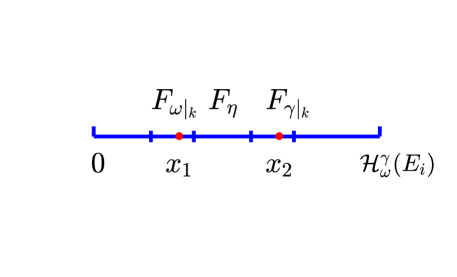
Figure 8. ${{\boldsymbol{\omega}}}$ and ${{\boldsymbol{\gamma}}}$ are not adjacent.

Then there is a cylinder ${\boldsymbol{\eta}}=\omega_{1}+\dots+\omega_{k-1}+\eta_{k}$ between ${\boldsymbol{\omega}}|_{k}$ and ${\boldsymbol{\gamma}}|_{k}$, so

$$\|x_{1}-x_{2}\|\geq\text{diam}~{}F_{\boldsymbol{\eta}}\geq h\cdot(q^{-\alpha/d})^{k},$$

where $h=\min\{{\mathcal{H}}_{\omega}^{\alpha}(E_{i});~{}i=1,\dots,N\}$. Since $x_{1}$ and $x_{2}$ belong to $\rho([\omega_{1}\omega_{2}\dots\omega_{k-1}])$ and denote ${\boldsymbol{\omega}}_{*}=\omega_{1}+\dots+\omega_{k-1}$, the images of $x_{1}$ and $x_{2}$ under $\pi_{i}\circ\rho_{i}^{-1}$, which denote by $y_{1}$ and $y_{2}$, respectively, belong to $\pi_{i}([{{\boldsymbol{\omega}}}_{*}])=E_{{{\boldsymbol{\omega}}}_{*}}$. Then we have

(4.7) $$\begin{split}\|y_{1}-y_{2}\|_{\omega}&\leq\text{diam}_{\omega}E_{{\boldsymbol{\omega}}^{*}}\leq\big{(}\text{max}_{1\leq m\leq N}\text{ diam}_{\omega}E_{i}\big{)}\cdot q^{-\frac{k-1}{d}}\\ &=D\cdot q^{1/d}\cdot(q^{-1/d})^{k}\leq D\cdot q^{1/d}\cdot(1/h)^{\frac{d}{\alpha}}\|x_{1}-x_{2}\|^{\frac{1}{\alpha}},\end{split}$$

where $D=\max_{1\leq i\leq N}\text{ diam}_{\omega}E_{i}.$

Now, we consider the case that ${{\boldsymbol{\omega}}}_{k}$ and ${{\boldsymbol{\gamma}}}_{k}$ are adjacent. (See Figure 9 (left).)

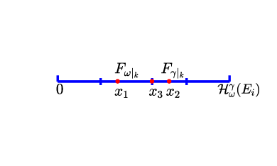
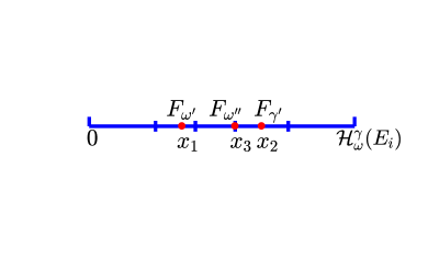
Figure 9. ${{\boldsymbol{\omega}}}$ and ${{\boldsymbol{\gamma}}}$ are adjacent.

Let $x_{3}$ be the intersection of $F_{{\boldsymbol{\omega}}|_{k}}$ and $F_{{\boldsymbol{\gamma}}|_{k}}$. Let $k^{\prime}$ be the smallest integer such that $x_{1}$ and $x_{3}$ belong to different cylinders of rank $k^{\prime}$, say, $x_{1}\in\rho_{i}([{\boldsymbol{\omega}}^{\prime}])$ and $x_{3}\in\rho_{i}([{\boldsymbol{\omega}}^{\prime\prime}])$ (see Figure 9 (right)), then $\|x_{1}-x_{3}\|\geq\text{diam}~{}F_{{\boldsymbol{\omega}}^{\prime\prime}}$ since $x_{3}$ is an endpoint. Let $y_{3}=\psi_{i}(x_{3})$. Similar to Case 1, we have

$$\|y_{1}-y_{3}\|_{\omega}\leq D\cdot q^{1/d}\cdot(1/h)^{\frac{d}{\alpha}}\|x_{1}-x_{3}\|^{\frac{1}{\alpha}}.$$

By the same argument, we have

$$\|y_{2}-y_{3}\|_{\omega}\leq D\cdot q^{1/d}\cdot(1/h)^{\frac{d}{\alpha}}\|x_{2}-x_{3}\|^{\frac{1}{\alpha}}.$$

Hence, by the fact $x_{3}$ is located between $x_{1}$ and $x_{2}$,

(4.8) $$\begin{split}\|y_{1}-y_{2}\|_{\omega}&\leq\beta\cdot\text{ max}\{\|y_{1}-y_{3}\|_{\omega},\|y_{3}-y_{2}\|_{\omega}\}\\ &\leq\beta\cdot D\cdot q^{1/d}\cdot(1/h)^{\frac{d}{\alpha}}\cdot\text{max }\{\|x_{1}-x_{3}\|^{\frac{1}{\alpha}},\|x_{2}-x_{3}\|^{\frac{1}{s}}\}\\ &\leq\beta\cdot D\cdot q^{1/d}\cdot(1/h)^{\frac{d}{\alpha}}\cdot\|x_{1}-x_{2}\|^{\frac{1}{\alpha}},\end{split}$$

where the first inequality is from Proposition 2.1 (iv).

Therefore, (4.7) and (4.8) verify the $1/\alpha$- Hölder continuity of $\psi_{i}$. $\Box$

References

- [1] S. Akiyama and B. Loridant, Boundary parametrization of planar self-affine tiles with collinear digit set, Sci. China Math., 53 (2010), pp. 2173–2194.
- [2] , Boundary parametrization of self-affine tiles, J. Math. Soc. Japan, 63 (2011), pp. 525–579.
- [3] R. Dai, X. and Y. Wang, Peano curves on connected self-similar sets, Unpublished note, (2010).
- [4] X.-r. Dai, H. Rao, and S.-q. Zhang, Space-filling curves of self-similar sets (II): Edge-to-trail substitution rule, ArXiv e-prints, (2015).
- [5] M. Dekking, Recurrent sets, Adv. in Math., 44 (1982), pp. 78–104.
- [6] K. Falconer, Fractal geometry,Mathematical Foundations and Applications, John Wiley, New York, 1990.
- [7] X.-G. He and K.-S. Lau, On a generalized dimension of self-affine fractals, Math. Nachr., 281 (2008), pp. 1142–1158.
- [8] L. Jun and Y.-M. Yang, On single-matrix graph-directed iterated function systems, J. Math. Anal. Appl., 372 (2010), pp. 8–18.
- [9] P.-G. Lemarié-Rieusset, Projecteurs invariants, matrices de dilatation, ondelettes et analyses multi-résolutions, Rev. Mat. Iberoamericana, 10 (1994), pp. 283–347.
- [10] B. t. Loridant, Topological properties of a class of cubic Rauzy fractals, Osaka J. Math., 53 (2016), pp. 161–219.
- [11] R. D. Mauldin and S. C. Williams, Hausdorff dimension in graph directed constructions, Trans. Amer. Math. Soc., 309 (1988), pp. 811–829.
- [12] H. Rao and S.-Q. Zhang, Space-filling curves of self-similar sets (I): iterated function systems with order structures, Nonlinearity, 29 (2016), pp. 2112–2132.
- [13] V. c. F. Sirvent, Space filling curves and geodesic laminations, Geom. Dedicata, 135 (2008), pp. 1–14.
- [14] , Space-filling curves and geodesic laminations. II: Symmetries, Monatsh. Math., 166 (2012), pp. 543–558.
- [15] P. Walters, An introduction to ergodic theory, vol. 79 of Graduate Texts in Mathematics, Springer-Verlag, New York-Berlin, 1982.