Natural Highways for End-of-Life Solutions in the LEO Region

Abstract

We present the main findings of a dynamical mapping performed in the Low Earth Orbit region. The results were obtained by propagating an extended grid of initial conditions, considering two different epochs and area-to-mass ratios, by means of a singly-averaged numerical propagator. It turns out that dynamical resonances associated with high-degree geopotential harmonics, lunisolar perturbations and solar radiation pressure can open natural deorbiting highways. For area-to-mass ratios typical of the orbiting intact objects, these corridors can be exploited only in combination with the action exerted by the atmospheric drag. For satellites equipped with an area augmentation device, we show the boundary of application of the drag, and where the solar radiation pressure can be exploited.

1 Introduction

Thanks to the effort made by scientists, public organizations and industries worldwide, there now exists a strong awareness on the value of preserving the circumterrestrial environment for future generations. The need of controlling the debris environment and limiting the growth of its population is addressed at several levels, which include, among others, long-term modeling, operational activities like collision avoidance operations and reentry campaigns, and mitigation actions.

For its strategic importance and its well-attested unstable evolution liou , the Low Earth Orbit (LEO) region is, in particular, subject to a thorough assessment by the community. The consequences of possible fragmentations in the long-term, active and passive debris removal campaigns, but also the new scenarios driven by the launch of mega constellations are the aspects where there is the strongest commitment rossi_frag , lewis . Besides the technological challenges, a renovated focus is put on the theoretical features which cannot be ignored.

We are here interested in passive disposal solutions, to be adopted at the end-of-life of a given mission. As very well known, the LEO region is one of the “Protected Regions” defined by international agreements ESA . It is formally defined as “the spherical shell that extends from the Earth’s surface up to an altitude of 2000 km”, and the mitigation guidelines require that “a space system operating in LEO shall be disposed of by reentry into the Earth’s atmosphere within 25 years after the end of the operational phase.”

Figure 1 shows the orbital distribution in terms of inclination $i$, semi-major axis $a$ and eccentricity $e$ of the objects in LEO with a mass greater than 100 kg, according to the ESA MASTER model MASTER . The most critical regions in LEO are located in the altitude ranges $[700:1000]$ km and $[1300:1600]$ km, where the orbits are mostly circular (with eccentricities usually lower than 0.02). In the same figure, we have indicated the mean altitude corresponding to a reentry in 25 years for circular orbits, thanks to the perturbation exerted by the atmospheric drag. It is clear from the figure that for most of the objects an impulsive de-orbiting strategy must be applied to comply with the guidelines. From the operational point of view, from a certain altitude onward (typically 1400 km), it is more convenient, in terms of propellant budget, to send a spacecraft to a graveyard orbit in a higher LEO. As a matter of fact, if we consider the payloads for which a maneuver must be applied, the percentage of compliance with the 25-year rule is actually very low, at less than a 15% FL17 -F17 . In order to avoid the accumulation of spent, uncontrolled spacecraft in a restricted region of space, which would lead inevitably to a significant number of collisions, it is mandatory to look for affordable solutions which ensure reentry within the Earth’s atmosphere in a reasonable time frame.

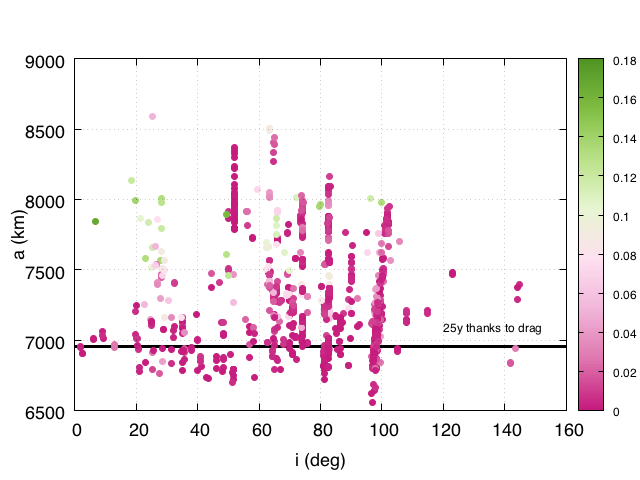
Figure 1: Orbital distribution in terms of inclination $i$ and semi-major axis $a$ of the objects in LEO with a mass greater than 100 kg, according to MASTER MASTER . The color bar reports the eccentricity of a given object.

The first step towards this direction is to understand if the dynamical perturbations in the region can drive the spacecraft towards natural reentry corridors. In this perspective, we present the simulations performed within the ReDSHIFT H2020 project aR17 on the dynamical behavior in LEO. The results corresponding to Medium Earth Orbits (MEO) and Geostationary Earth Orbits, performed within the ReDSHIFT H2020 project, can be found in Grecia_SD , and Colombo_SD , GC17 , respectively. General results on the whole circumterrestrial space, also obtained within the ReDSHIFT H2020 project, can be found in Grecia_Grecia .

To our knowledge, such an extensive and systematic exploration was never performed. The main objective is to detect “deorbiting highways”, associated with a significant change in eccentricity due to natural perturbations, apart from the atmospheric drag. The results are collected in a series of color maps, which describe at once whether a reentry is feasible, and, in such case, the required time and initial dynamical configuration.

This study provides a new insight on the dynamical effects caused by three different sources: the lunisolar gravitational attraction, the solar radiation pressure (SRP), and high-degree geopotential. At specific values of inclinations, these perturbations can foster the orbital decay, if a well-defined resonance condition is satisfied. Notice that resonances associated with these effects and the theoretical possibility to exploit them to lower the lifetime of spacecraft at the end-of-life were already theorized in the past (see, e.g., B1999 -B2001a ). Nonetheless, so far space agencies have conceived their application mainly for MEO (see, e.g., A16 ) and Highly Elliptical Orbits (see, e.g., C2014 ). The only work, as far as we know, which considered operational aspects of these natural leverages also for LEO is LetAl12 , in which however a very narrow range of initial conditions is analyzed.

In the work, two values of area-to-mass ratios are considered in order to show how the exploitation of a drag- or SRP-enhancing device might change the whole picture, but also to get a deeper understanding of the boundary between the realms of application of these two effects. A full analysis on the case of the sail is not considered here, but only the main features will be described. As a matter of fact, this topic deserves a specific focus, given also the copious literature which exists on the subject and the crucial interaction between atmospheric drag and solar radiation pressure.

A full understanding of the dynamics at stake in the most populated and operational region is the key starting point for many of the actions the community will or must take. The results can be exploited to design passive end-of-life solutions, to optimize the impulsive strategies aimed at reentering, and to support the roadmap for eventually taking advantage of a drag or a solar sail, but they could help also, e.g., in choosing the nominal orbits during the operational phase of a spacecraft, or for observational campaigns.

2 Numerical Simulation

The numerical simulation performed consists in propagating a series of initial conditions, which are representative of the whole LEO region, for 120 years, starting from two different initial epochs, namely, December 22, 2018 at 17:50:21 (JD 2458475.2433), and June 21, 2020 at 06:43:12 (JD 2459021.7800). They correspond to a December full Moon and a June new Moon solstice, where the longitude of the Sun with respect to the ecliptic plane is $\lambda_{S}\approx 270^{\circ}$ and $\lambda_{S}\approx 90^{\circ}$, respectively. On the second epoch a solar eclipse will occur. The choice of the initial epochs was suggested by the will of comparing, in a second step, the results of the numerical simulations with simpler, averaged, analytical models where the relative configuration of the Sun-Earth-Moon system was expected to play a role. In particular, the constraints set consisted in configurations

• close to solstices, so that the Earth rotation axis points towards the Sun;

• at a new or a full Moon, so that Sun, Earth and Moon are aligned;

• with the line of nodes of the lunar orbit possibly close to $0^{\circ}$, $90^{\circ}$, $180^{\circ}$ or $270^{\circ}$ with respect to the line containing the three bodies.

Similar to what done in A16 , during the 120 years time interval, the orbital evolution of semi-major axis, eccentricity, inclination, right ascension of the ascending node, argument of perigee $(a,e,i,\Omega,\omega)$ was recorded at a step of 1 day. Moreover, maximum and minimum values attained by semi-major axis, eccentricity and inclination were stored. The orbit was considered to have reentered into the atmosphere, whenever the altitude of perigee, say $h_{p}$, had decreased down to 300 km.

In the following, the details on the orbit propagator and on the initial conditions are given.

2.1 FOP

The numerical method used is the Fast Orbit Propagator (FOP) lAesa -aR09 , which is an accurate, long-term orbit predictor, based on the Long-term Orbit Predictor (LOP) jK86 . This singly-averaged formulation integrates the Lagrange or Gauss planetary equations for a set of orbital elements, which are non-singular for circular orbits and singular only for equatorial orbits. The numerical integrator is a multi-step, variable step-size and order integrator. The dynamical model accounts for the gravitational and non-gravitational perturbations stemming from the Earth, the Moon, and the Sun, namely,

• geopotential harmonics (up to degree and order 5):

• lunisolar perturbations;

• atmospheric drag;

• solar radiation pressure, including shadows.

To expedite the computations, the perturbations are analytically averaged over the mean anomaly of the satellite. For tesseral resonant effects (located at specific values of semi-major axis, where there exists a commensurability between the satellite’s mean motion and the Earth’s rotation rate), a partial averaging procedure is applied to retain only the long-periodic perturbations associated with these harmonics. The positions of the Moon and the Sun, which are held constant during the averaging process, are determined by means of accurate analytical ephemerides. The SRP effect is represented by the cannonball model, accounting also for shadowing intervals. The shadows are modeled as solar occultations, with a cylindrical model. The algorithm is based on the assumption that the Sun is a point at infinity and that the spacecraft and the Sun are frozen during the occultation. The atmospheric drag is applied for altitudes below 1500 km, adapting the Jacchia-Roberts density model assuming an exospheric temperature of 1000 K and a variable solar flux at 2800 MHz (obtained by means of a Fourier analysis of data corresponding to the interval 1961-1992). To average the disturbing accelerations associated with solar radiation pressure and atmospheric drag, a standard 8th-order Gaussian quadrature method is used. FOP was widely validated in the past lAesa , and thus no additional analysis was needed for the present work. Notice that in LEO none of the effects considered in the dynamical model can be neglected.

2.2 Grid Definition

The grid of initial orbital elements explored is shown in Table 1. Note that the LEO region is usually defined for circular orbits up to $2000$ km in altitude, which is lower than the maximum value of semi-major axis adopted here. On the one hand, this choice is justified by the fact that orbits with larger semi-major axes but also higher eccentricities have perigee altitudes falling below that limit. On the other hand, a precise understanding of the dynamics just beyond $2000$ km is important for the long-term stability of graveyard orbits.

The range of eccentricity allowed is such that the initial perigee is higher than 300 km. Moreover, to depict accurately the situation of the most critical regions in LEO, besides the refinement in semi-major axis displayed in the table, a finer step in eccentricity, namely, $\Delta e=10^{-3}$, was adopted for $a<R_{E}+1600$ km and $e<0.01$, being $R_{E}=6378.1363$ km the mean radius of the Earth.

Concerning the step-size used for the longitude of the ascending node and the argument of perigee, the standard definition adopted was $90^{\circ}$, but for some specific values of $(a,e,i)$ a higher-resolution exploration was performed, taking $\Delta\Omega=10^{\circ}$ and $\Delta\omega=10^{\circ}$, both $\Omega$ and $\omega$ in the range $[0:360)$ deg.

Table 1: Grid of initial conditions in semi-major axis $a$, eccentricity $e$ and inclination $i$ for the exploration performed. $R_{E}=6378.1363$ km is the radius of the Earth.

$a$ (km)	$\Delta a$ (km)	$e$	$\Delta e$	$i$ (deg)	$\Delta i$ (deg)
$[500:700]$ + $R_{E}$	$50$	$[0:0.28]$	$0.01$	$(0:120]$	$2$
$[700:1000]$ + $R_{E}$	$20$	$[0:0.28]$	$0.01$	$(0:120]$	$2$
$[1000:1300]$ + $R_{E}$	$50$	$[0:0.28]$	$0.01$	$(0:120]$	$2$
$[1300:1600]$ + $R_{E}$	$20$	$[0:0.28]$	$0.01$	$(0:120]$	$2$
$[1600:2000]$ + $R_{E}$	$50$	$[0:0.28]$	$0.01$	$(0:120]$	$2$
$[2000:3000]$ + $R_{E}$	$100$	$[0:0.28]$	$0.01$	$(0:120]$	$2$

For all the initial conditions, the drag coefficient was set to $C_{D}=2.1$, while the reflectivity coefficient to $C_{R}=1$ or $C_{R}=2$. For the area-to-mass ratio, the standard value used was $A/m=0.012$ m${}^{2}/$kg, which reflects the average value of the orbiting intact population. This value was the result of a thorough analysis carried out on the MASTER catalogue Colombo_SD . For the 2020 epoch, the simulations were repeated assuming $C_{R}=1$ and $A/m=1$ m${}^{2}/$kg, which can be considered as a realistic value achievable for small satellites equipped with a drag- or SRP-enhancing device.

The total number of initial conditions simulated, not accounting for the specific analysis described in Sec. 3.3, is 3.6 millions.

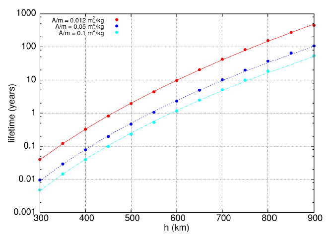
Figure 2: Lifetime corresponding to different altitude values for circular LEO and different area-to-mass ratios, obtained by propagation with DROMO (see, e.g., hU16 ).

3 Numerical Results

The analysis presented is based on the study of the lifetime and the maximum eccentricity computed for each initial condition in the grid. The goal is to build, for the first time, a detailed map of the dynamical behavior in the whole LEO region. As a matter of fact, at altitudes where the effect of the drag is not dominant, the lifetime of an orbit can vary significantly only on account of eccentricity excitations. Speaking of unstable orbits, we will always refer to this behavior. In general, focusing for the moment our analysis on the lower value of area-to-mass ratio, beyond the drag realm, the maximum variation computed in semi-major axis is of the order of tens of km, and it is due to tesseral effects EK97 -GC15 . The maximum change in inclination is generally up to 1 degree, apart from specific retrograde orbits for which variations can reach up to 4 degrees.

3.1 Lifetime

For low values of area-to-mass ratio, the lifetime estimates corresponding to circular LEO (within the limits of the solar flux predictability) are generally known, but , as far as we know, complete and detailed analyses on elliptic orbits are not available. As a reference, in Figure 2, we show the lifetime of circular LEO corresponding to different values of altitude and area-to-mass ratio of the satellite, obtained from propagations with DROMO (see, e.g., hU16 ) assuming the NRLMSISE–00 atmospheric model with the solar flux defined by ESA’s model ESA . Note that, as seen in the figure, beyond $a=R_{E}+800$ km a spacecraft with $A/m=0.012$ m${}^{2}/$kg on a circular orbit takes more than 100 years to reenter.

Our first step in the analysis of the results is to discriminate between the cases which can naturally comply with the 25-year rule, thanks to some perturbations, and those which cannot. The general behavior computed for $A/m=0.012$ m${}^{2}/$kg (2020 epoch) is shown in Figure 3. For each initial condition considered, we look for the minimum value of eccentricity, as a function of the semi-major axis, which guarantees a lifetime of at most 25 years (blue line in the figure). At the same time, we identify the minimum value of eccentricity, for any value of inclination in the range explored and for each given semi-major axis, which ensures to reenter within the assumed 120 years window of propagation (red line in the figure).

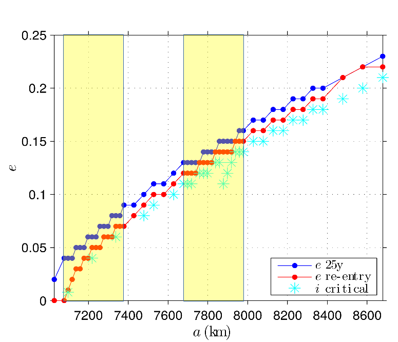
Figure 3: As a function of the semi-major axis, the minimum value of eccentricity required to reenter in 25 years (blue curve), and in less than 120 years (red curve), assuming $A/m=0.012$ m${}^{2}/$kg, and $\Omega=180^{\circ}$ and $\omega=0^{\circ}$ and the initial epoch 2020. The cyan stars represent cases where perturbations different from drag facilitate the reentry at specific values of inclination (see text for details). In yellow, the most populated altitudes.

We stress that, for the standard value of area-to-mass ratio, in LEO the reentry cannot be achieved without the action exerted by the atmospheric drag, whose effect, as known, is to decrease both the semi-major axis and the eccentricity. To this end, the initial pericenter altitude must be lower than a given threshold, which depends on the semi-major axis. For the whole range of eccentricity explored, considering initial values of semi-major axis such that $a>R_{E}+800$ km, the minimum pericenter altitude required to reenter spans from about $580$ km down to about $350$ km, for increasing semi-major axis values. The cyan stars in Figure 3 represent specific cases where perturbations different from drag facilitate the reentry (but not on their own). In other words, depending on the initial configuration, i.e., on the initial values of $(i,\Omega,\omega)$, given $a$, a reentry could be achieved at a lower value of eccentricity. In the following, we will refer to these specific inclinations as resonant inclinations; the reason for this will be clarified in Section 4.

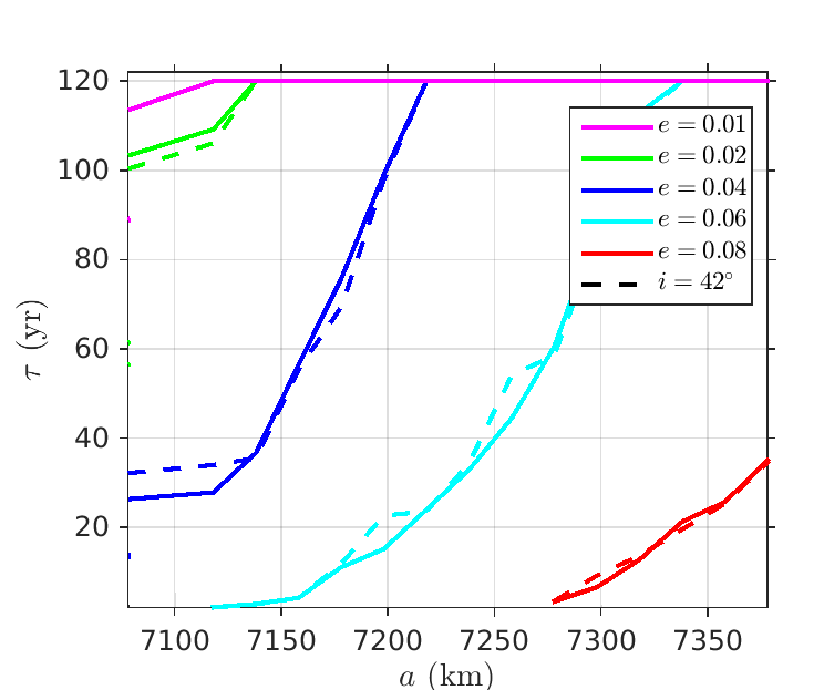
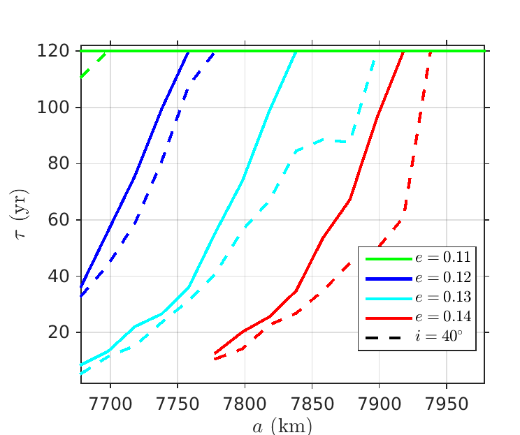
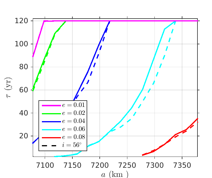
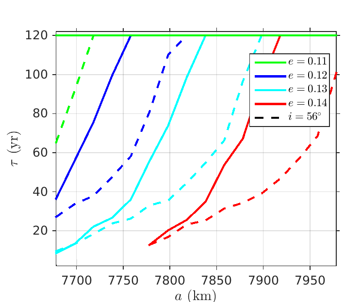
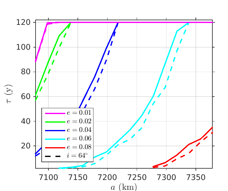
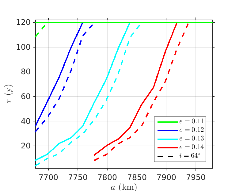
Figure 4: Comparison of the lifetime computed in correspondence of a resonant inclination (dashed curve) or non-resonant inclination (solid curves). Left: $a\in[7078.14:7378.14]$ km. Right: $a\in[7678.14:7978.14]$ km. Top: $i=40^{\circ}$. Middle: $i=56^{\circ}$. Bottom: $i=64^{\circ}$. Initial epoch 2020, $C_{R}(A/m)=0.024$ m${}^{2}/$kg, $\Omega=0^{\circ}$, $\omega=90^{\circ}$.

In Figure 4, we show the standard lifetime curves computed for two different ranges of semi-major axis and high-enough values of eccentricity, together with the lifetime curves computed in the same regions for three of the resonant inclination values detected, namely, $40^{\circ}$, $56^{\circ}$ and $64^{\circ}$. The improvement in the reentry times in the cases where the resonant inclinations are exploited (dashed lines) is noticeable, when the eccentricity is sufficiently high for the drag to be effective. From the figure, it can be seen that for $a\in[7078.14:7378.14]$ km, the effect of the atmospheric drag combined with lunisolar perturbations, geopotential or solar radiation pressure can be exploited starting from $e>0.02$, while for $a\in[7678.14:7978.14]$ km, the eccentricity must be as high as $e>0.11$. Notice also that in the latter case the reduction in lifetime is much larger, mainly because the eccentricity and the semi-major axis values correspond to a lower pericenter altitude and thus a stronger atmospheric effect.

As a further illustration of the dynamical interplay between the drag and one of the other perturbations considered, in Figures 5–6, we compare the evolution in time of the eccentricity and the pericenter altitude for $i=56^{\circ}$, $\Omega=0^{\circ}$, $\omega=90^{\circ}$, epoch 2020, $C_{R}(A/m)=0.012$ m${}^{2}/$kg, for two values of semi-major axis and eccentricity ($a=7300.14$ km, $e=0.06$ and $a=7800.14$ km, $e=0.13$), when the lunisolar perturbation is included and when it is not in the numerical propagation. In both examples, the reduction in lifetime is due to a slight, which could appear negligible, increase in eccentricity (see middle panels in both figures). This variation takes place after several years from the initial epoch and yields a value which is lower than the initial one. What matters, however, is the effect on the pericenter altitude, taking into account also the fact that the drag has, in the meantime, reduced the semi-major axis by an amount of 50-100 km in both examples. Recall that the atmospheric drag depends on the atmospheric density, which behaves exponentially. The lower the altitude, the stronger the effect.

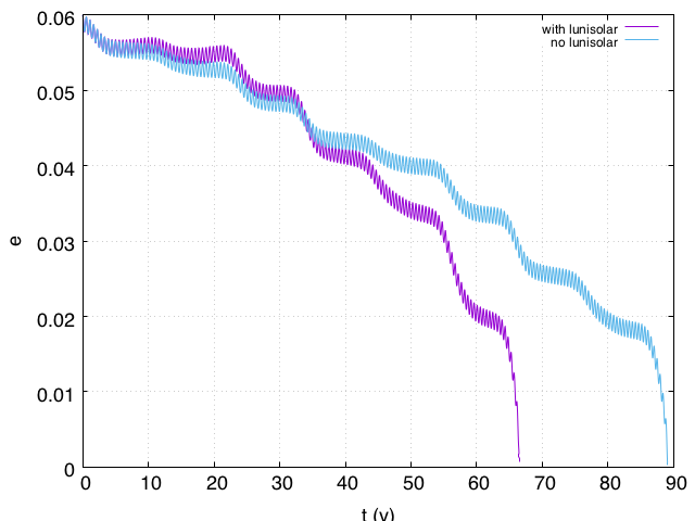
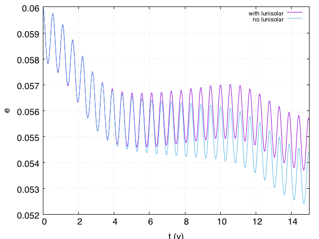
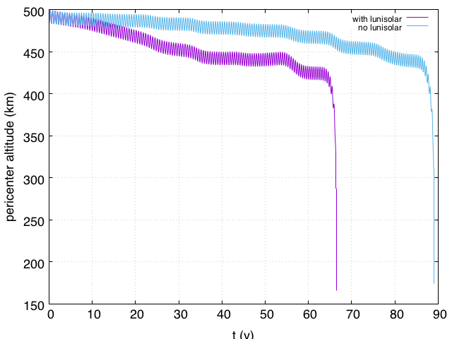
Figure 5: Comparison of the lifetime computed when the effect of the drag is combined with a lunisolar gravitational resonance (purple), and when lunisolar perturbations do not act (blue). Left: eccentricity behavior in time. Middle: detailed behavior at the time when the relative eccentricity increase takes place. Right: pericenter altitude behavior in time. Initial condition: $a=7300.14$ km, $e=0.06$, $i=56^{\circ}$, $\Omega=0^{\circ}$, $\omega=90^{\circ}$, epoch 2020, $C_{R}(A/m)=0.012$ m${}^{2}/$kg.

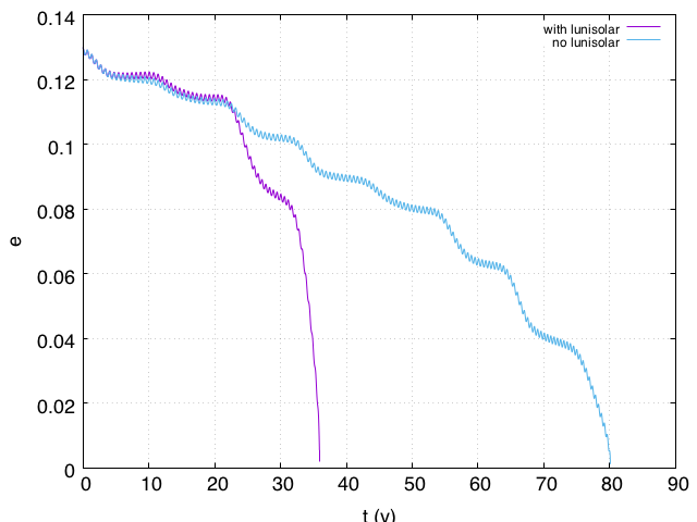
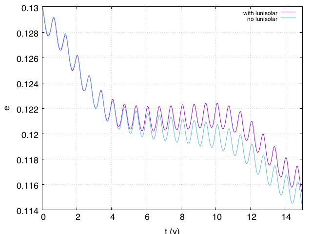
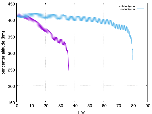
Figure 6: Comparison of the lifetime computed when the effect of the drag is combined with a lunisolar gravitational resonance (purple), and when lunisolar perturbations do not act (blue). Left: eccentricity behavior in time. Middle: detailed behavior at the time when the relative eccentricity increase takes place. Right: pericenter altitude behavior in time. Initial condition: $a=7800.14$ km, $e=0.13$, $i=56^{\circ}$, $\Omega=0^{\circ}$, $\omega=90^{\circ}$, epoch 2020, $C_{R}(A/m)=0.012$ m${}^{2}/$kg.

3.2 Cartography

To visualize more in detail the dynamical mechanisms, we build contour maps of both the lifetime and the maximum eccentricity attained in 120 years, as a function of the initial inclination and altitude of perigee or of the initial inclination and eccentricity, for each value of initial semi-major axis and for each of the 16 initial $(\Omega,\omega)$ configurations. They represent what we call the cartography of the LEO region. Note that, at the end of the ReDSHIFT project, all the maps will be available on the ReDSHIFT website (http://redshift-h2020.eu/).

Some illustrative plots for increasing values of initial semi-major axis, considering the same initial $(\Omega,\omega)$ combination and initial epoch are shown in Figure 7 and Figure 8, for a standard value of the area-to-mass ratio, as a function of the initial inclination and eccentricity. The two figures represent the behavior in terms of maximum eccentricity and corresponding lifetime, respectively. Analogous plots are displayed in Figure 9 and Figure 10 for the same initial epoch and $A/m=1$ m${}^{2}/$kg.

Looking to the maximum eccentricity behavior, for the majority of the initial eccentricity values the variation in 120 years is not significant; i.e., the color associated with a given initial eccentricity corresponds, in general, to the same initial value. There exist, however, interesting well-defined regions where the color associated with a given initial inclination and eccentricity is ‘brighter’ or ‘darker’. The effect is much more evident for the high value of area-to-mass ratio (Figure 9), but an accurate look can detect the same feature also for the lower area-to-mass ratio case. For instance, there are ‘yellower’ bands or islands in correspondence of $i\approx 40^{\circ}$ or $i\approx 80^{\circ}$ on the fourth and the last line of plots in Figure 7. In all the panels of the same figure, similar behaviors can be noticed.

Focusing on Figure 8, where the colorbar reports the lifetime, we can see that for high values of semi-major axis, the variation in eccentricity just noticed for the standard value of area-to-mass ratio is not sufficient to provoke a reduction in lifetime. In other words, perturbation effects different from the atmospheric drag can be exploited only if the eccentricity is high enough, depending on the value of semi-major axis. This is the reason why most of the plots is black, apart from a narrow band corresponding to high values of eccentricity. The width of this eccentricity band is much larger for the higher value of area-to-mass ratio (see Figure 10).

To better clarify this point, in Figure 11, for $a=R_{E}+1400$ km and the standard area-to-mass ratio value, we show the lifetime behavior as a function of the initial inclination and value of pericenter altitude for all the 16 $(\Omega,\omega)$ configurations explored. From this figure, we can see that to adopt the initial pericenter altitude instead of the initial eccentricity as reference parameter helps in understanding how deep the spacecraft should enter into the atmosphere to eventually reenter. Moreover, in each plots of the figure bright or dark bands stand out in correspondence of well-defined values of inclinations, as it was already clear for the high area-to-mass ratio case from Figure 9. These are the resonant inclinations, associated with the cyan stars in Figure 3. According to whether a resonant inclination is associated with a lighter or darker shade than that of the neighboring points, the lifetime is shorter or longer, i.e., the eccentricity experiences a growth or a reduction. These are the regions where the perturbation exerted by the geopotential or by the Moon or by the Sun (both gravitationally or as solar radiation pressure) are able to alter the general behavior. Finally, the initial configuration is crucial to obtain a reduction or an increase in lifetime.

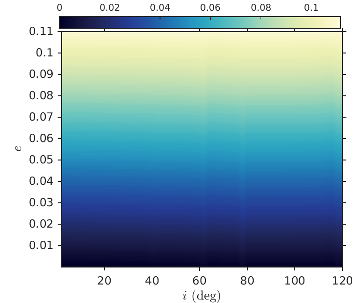
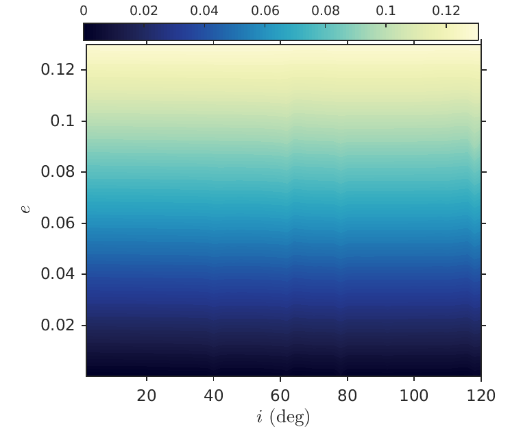
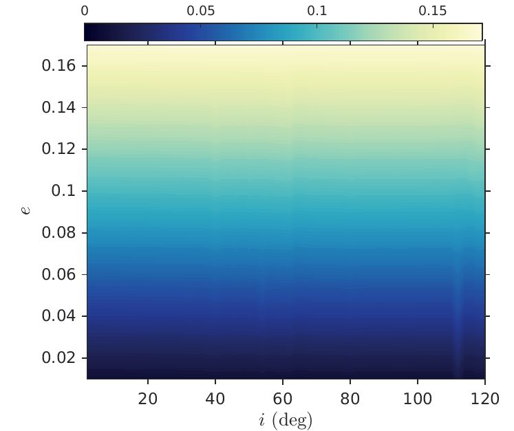
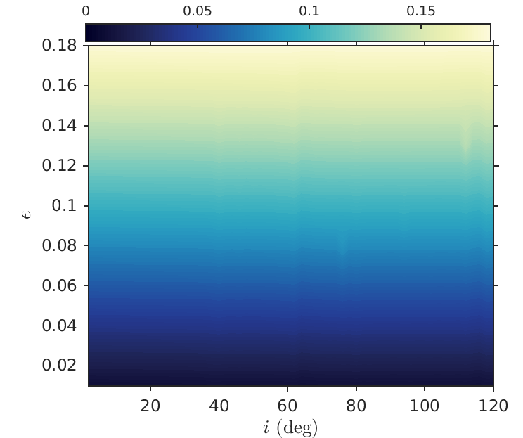
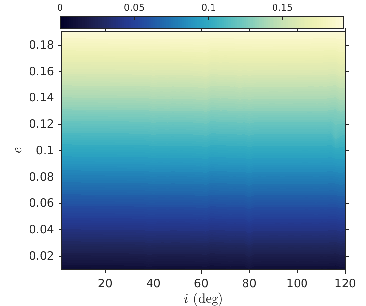
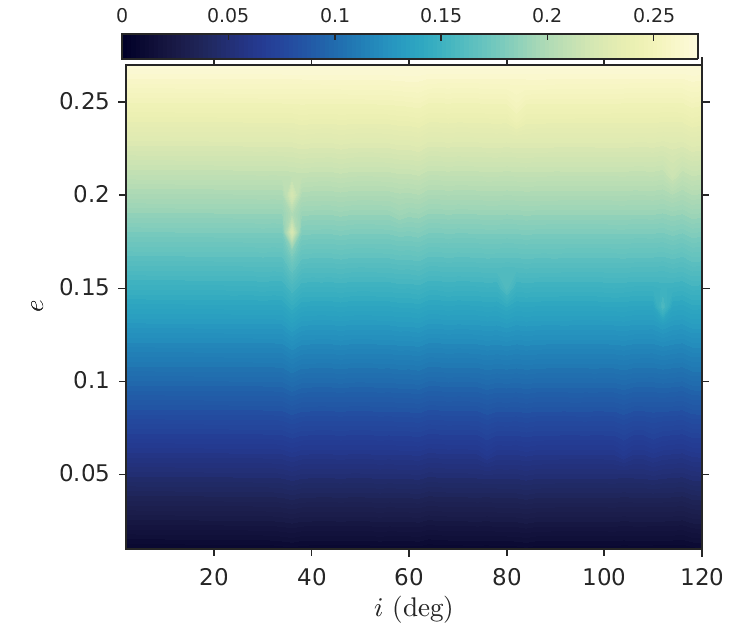
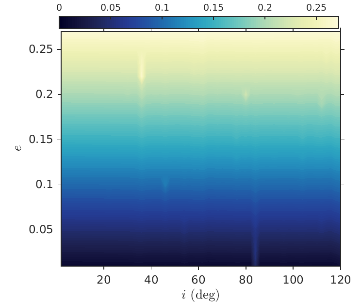
Figure 7: Maximum eccentricity computed (color bar) as a function of initial inclination and eccentricity for the initial epoch 2020 and $C_{R}(A/m)=0.024$ m${}^{2}/$kg, assuming $\Omega=0^{\circ}$ and $\omega=0^{\circ}$ at the initial epoch. Each plot depicts the behavior computed starting from a different value of initial semi-major axis. From the top left to the bottom right: $a=R_{E}+700$ km to $a=R_{E}+3000$ km at a step of 100 km.

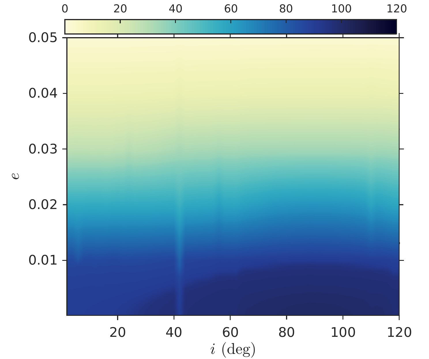
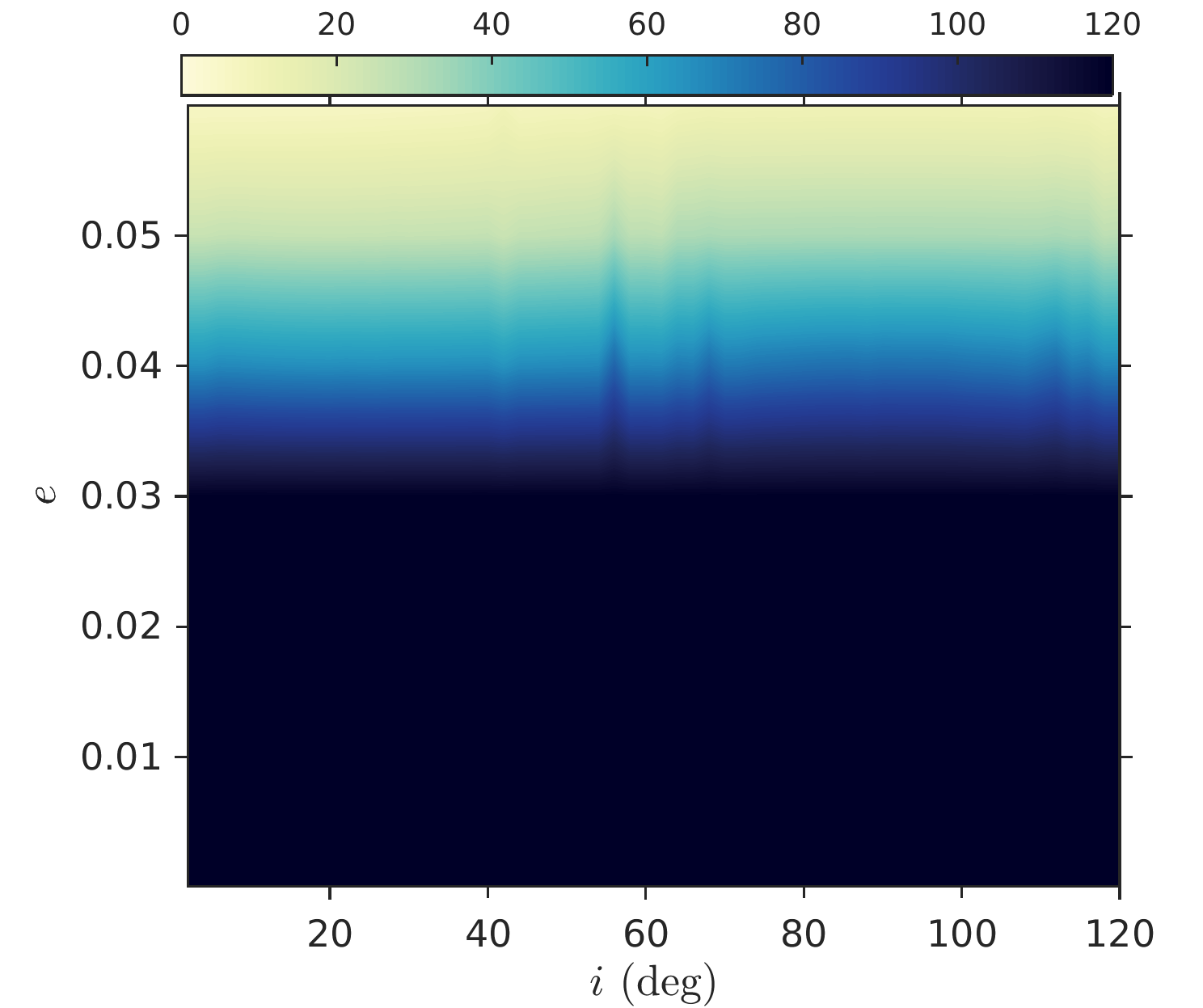
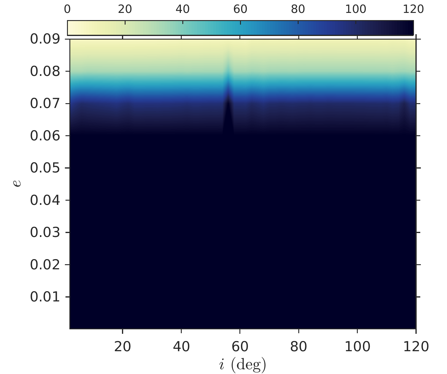
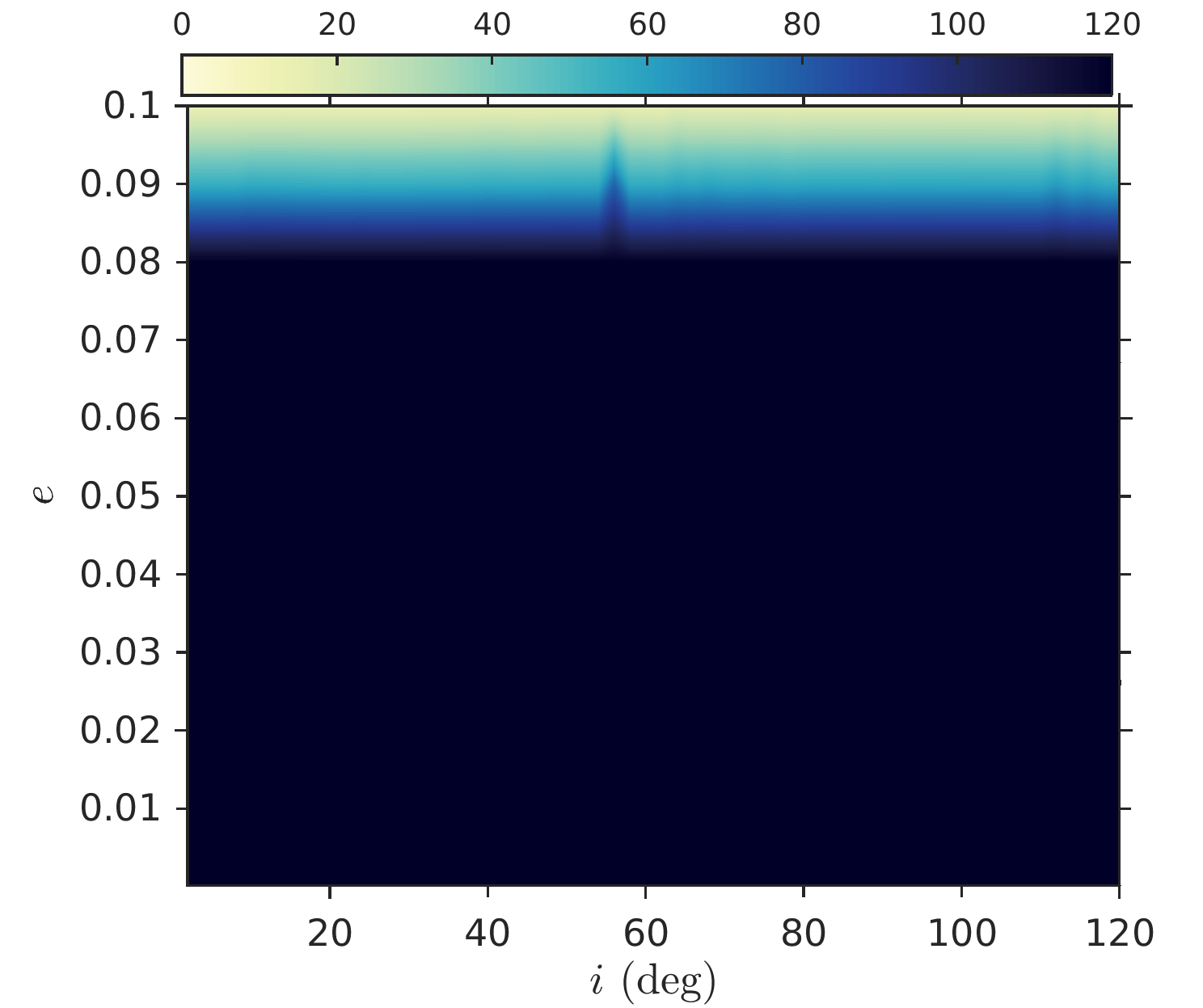
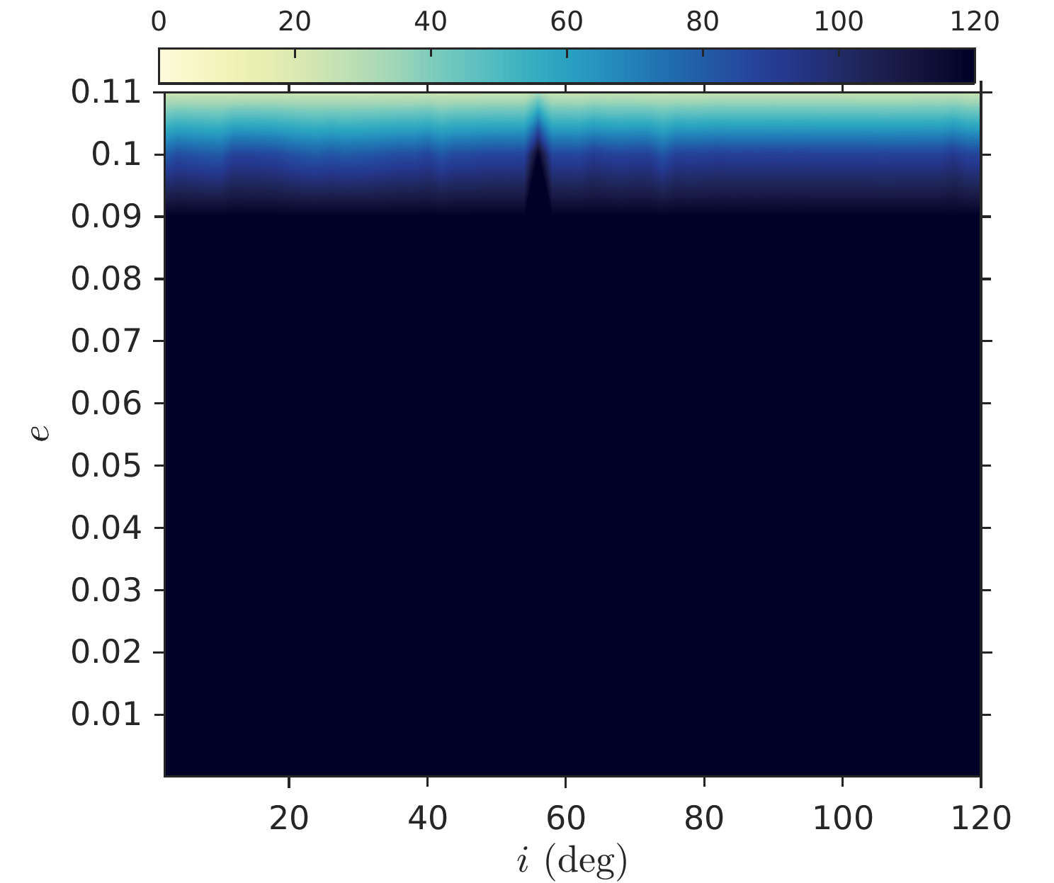
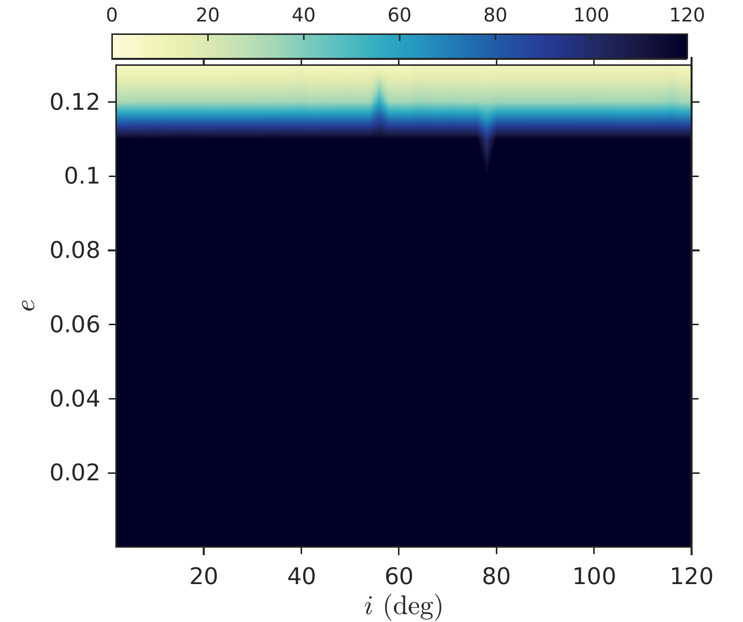
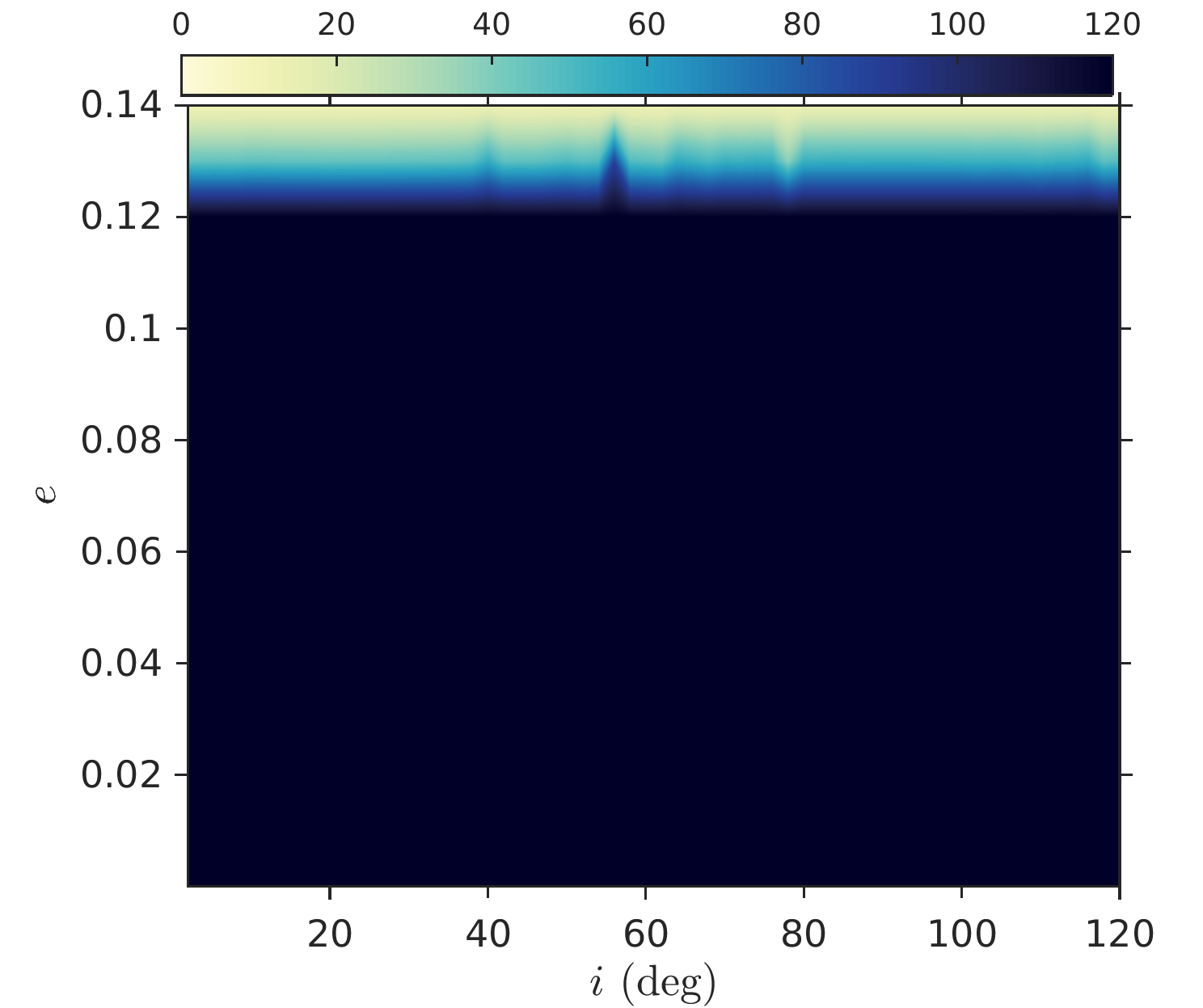
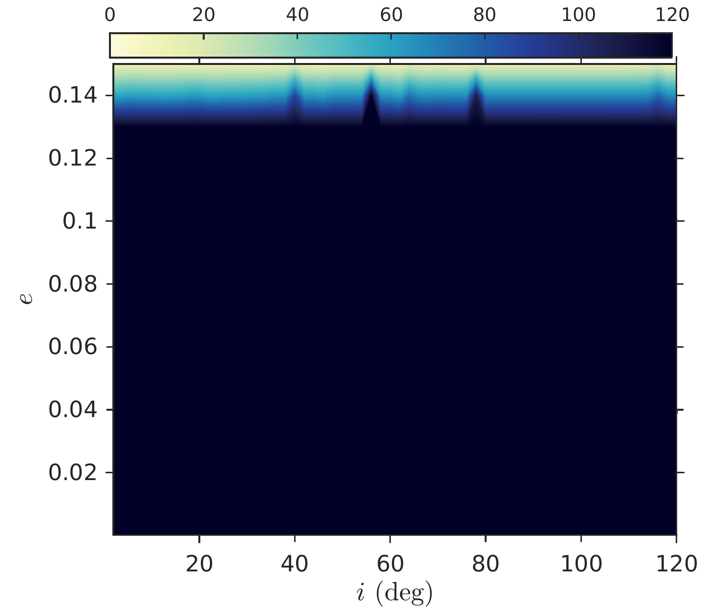
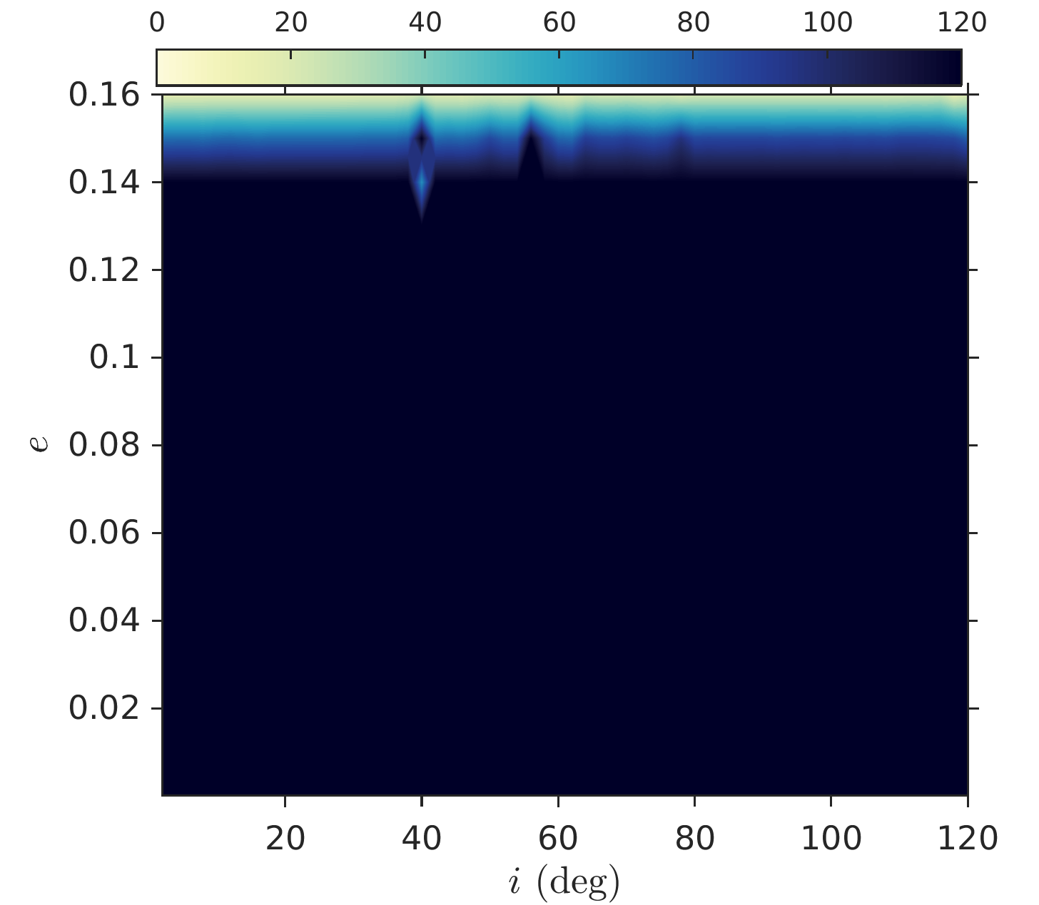
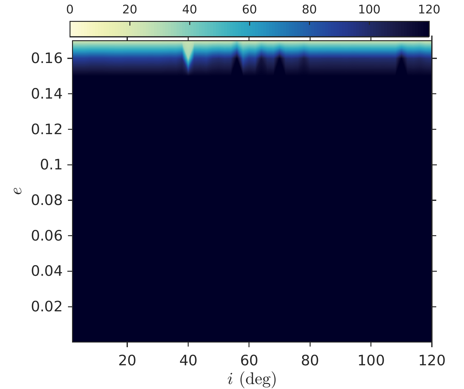
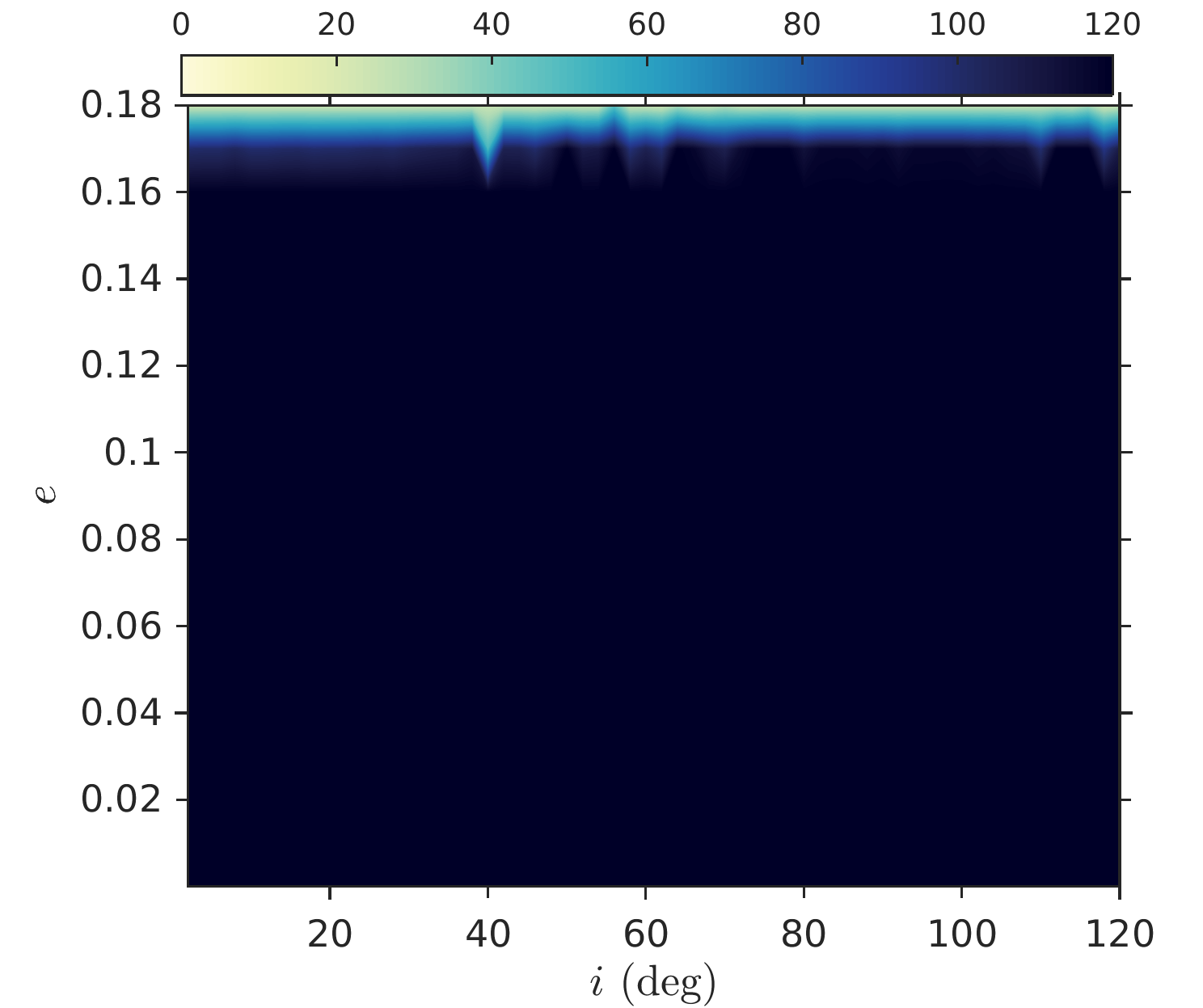
Figure 8: Lifetime computed (color bar) as a function of initial inclination and eccentricity for the initial epoch 2020 and $C_{R}(A/m)=0.024$ m${}^{2}/$kg, assuming $\Omega=0^{\circ}$ and $\omega=0^{\circ}$ at the initial epoch. Each plot depicts the behavior computed starting from a different value of initial semi-major axis. From the top left to the bottom right: $a=R_{E}+700$ km to $a=R_{E}+1800$ km at a step of 100 km. For higher values of semi-major axis, the range of eccentricity allowing for a reentry is as narrow as the last plot shown, or even less.

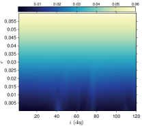
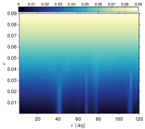
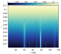
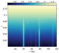
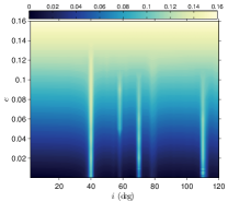
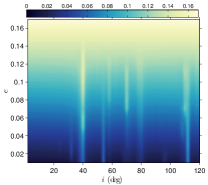
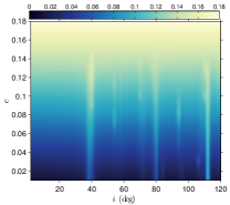
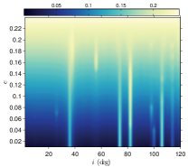
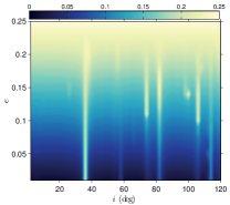
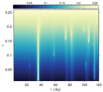
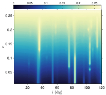
Figure 9: Maximum eccentricity computed (color bar) as a function of initial inclination and eccentricity for the initial epoch 2020 and $C_{R}(A/m)=1$ m${}^{2}/$kg, assuming $\Omega=0^{\circ}$ and $\omega=0^{\circ}$ at the initial epoch. Each plot depicts the behavior computed starting from a different value of initial semi-major axis. From the top left to the bottom right: $a=R_{E}+700$ km to $a=R_{E}+3000$ km at a step of 100 km.

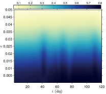
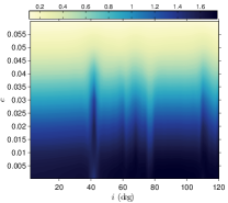
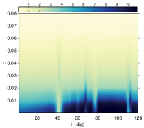
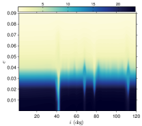
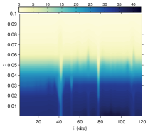
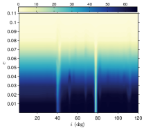
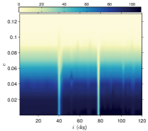
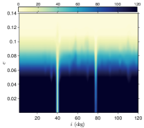
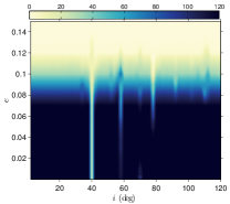
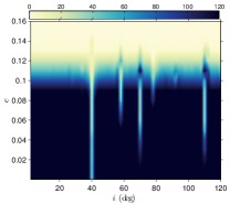
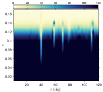
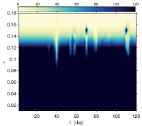
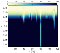
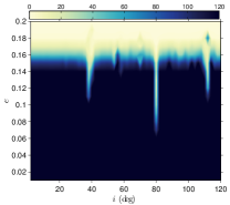
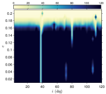
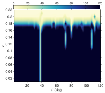
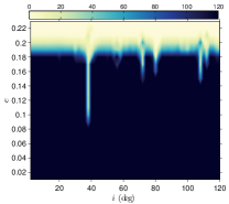
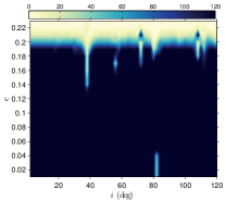
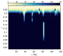
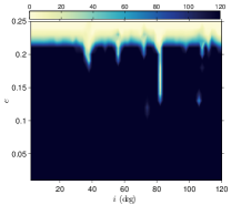
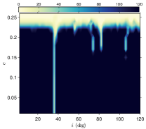
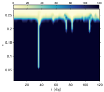
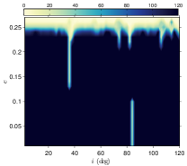
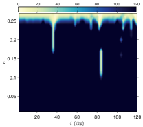
Figure 10: Lifetime computed (color bar) as a function of initial inclination and eccentricity for the initial epoch 2020 and $C_{R}(A/m)=1$ m${}^{2}/$kg, assuming $\Omega=0^{\circ}$ and $\omega=0^{\circ}$ at the initial epoch. Each plot depicts the behavior computed starting from a different value of initial semi-major axis. From the top left to the bottom right: $a=R_{E}+700$ km to $a=R_{E}+3000$ km at a step of 100 km.

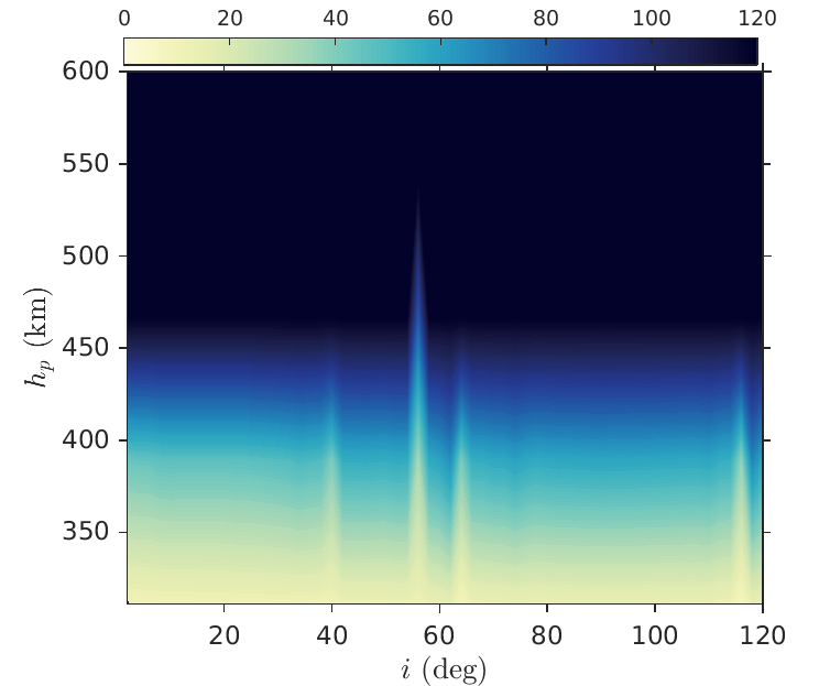
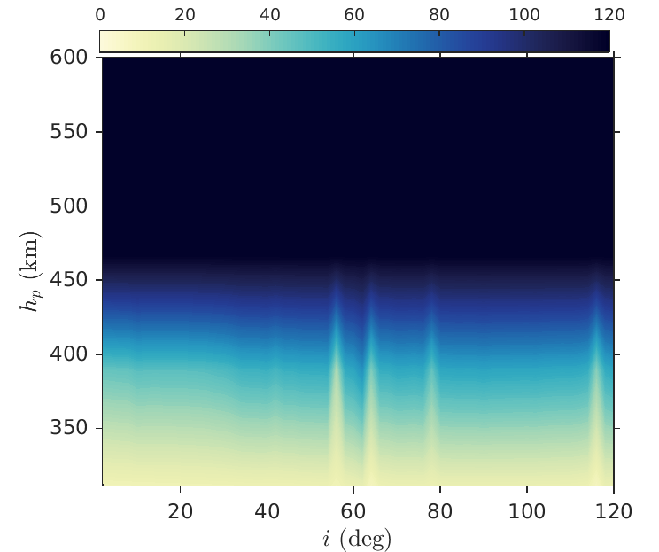
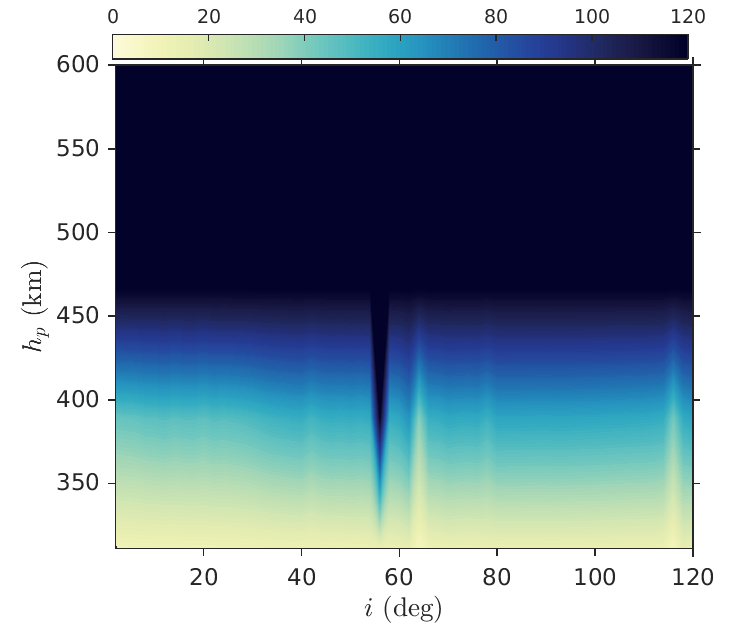
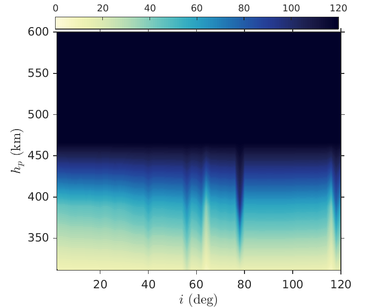
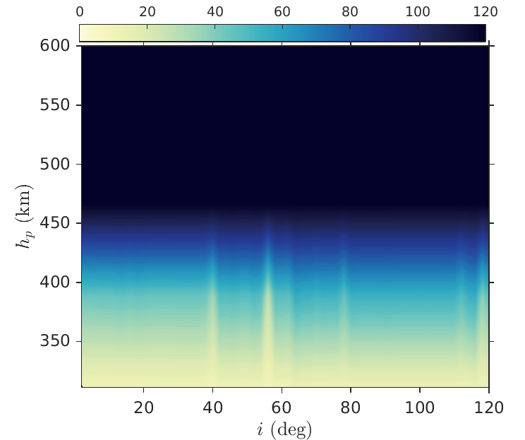
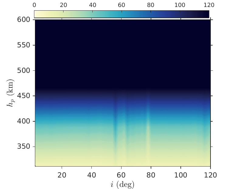
Figure 11: Lifetime computed (color bar) as a function of initial inclination and altitude of pericenter for the initial epoch 2020 and $C_{R}(A/m)=0.024$ m${}^{2}/$kg, assuming $a=R_{E}+1400$ km for different initial $(\Omega,\omega)$ configurations. From top to bottom: $\Omega=0^{\circ}$, $\Omega=90^{\circ}$, $\Omega=180^{\circ}$, $\Omega=270^{\circ}$. From left to right: $\omega=0^{\circ}$, $\omega=90^{\circ}$, $\omega=180^{\circ}$, $\omega=270^{\circ}$.

Concerning the results for the high value of area-to-mass ratio considered, a complete analysis of the results is beyond the scope of this work, but it is worth stressing that the simulations revealed that the exploitation of a drag sail might be successful also for circular orbits up to an altitude of about 1200 km, if we allow a reentry time as long as 50 years; up to about 1050 km, if we aim at complying with the 25-year rule. Apart from the behavior displayed in Figure 10, we provide further examples for a different initial $(\Omega,\omega)$ initial configuration in Figure 13, where we show the lifetime computed for $a=R_{E}+800$ km, $a=R_{E}+1000$ km and $a=R_{E}+1200$ km. In Fig. 12, we show the pericenter and apocenter altitudes corresponding to a reentry in less than 25 years for both values of area-to-mass ratio. Notice the higher pericenter values in the case of an enhanced area-to-mass ratio and the behavior of quasi-circular orbit in the same case.

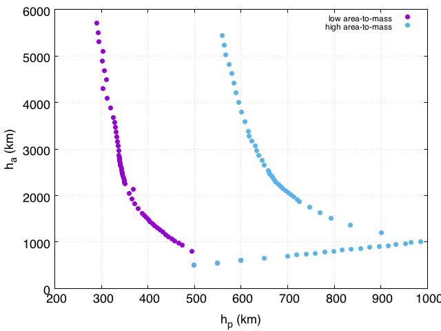
Figure 12: Pericenter $h_{p}$ and apocenter $h_{a}$ (km) required to reenter in 25 years for the two values of area-to-mass ratio considered in this study.

From the point of view of the orbital dynamics, the two main differences between the usage of a drag or a solar sail are the altitude where they can be exploited, and the fact that the drag sail can be considered for any value of inclination. Instead, in order to properly exploit the SRP perturbation (i.e., the solar sail) the corresponding resonant inclination bands shall be targeted. In this case, for circular orbits, it is possible to achieve reentry for values of semi-major axis up to about 2900 km (see third panel in the last line of Figure 10). An example of the SRP effect is provided in Figure 14, where we show the long-term evolution of the eccentricity for $C_{R}(A/m)=1$ m${}^{2}/$kg, $a=R_{E}+1950$ km, $e=0.02$, $\Omega=270^{\circ}$, $\omega=270^{\circ}$, and two different values of initial inclination at the initial epoch 2020. In the case of the resonant inclination, $i=80^{\circ}$, the reentry can be achieved. In Figure 15, we compare the maximum eccentricity behavior for a same initial condition for a satellite which is not equipped with a sail, and a satellite which is. The opening of strong reentry corridors at the resonant inclinations are clearly evident in the area-enhanced case of the right panel.

The number of reentry solutions computed for the same initial epoch 2020 for the two values of area-to-mass ratio is 83402 and 490920, respectively.

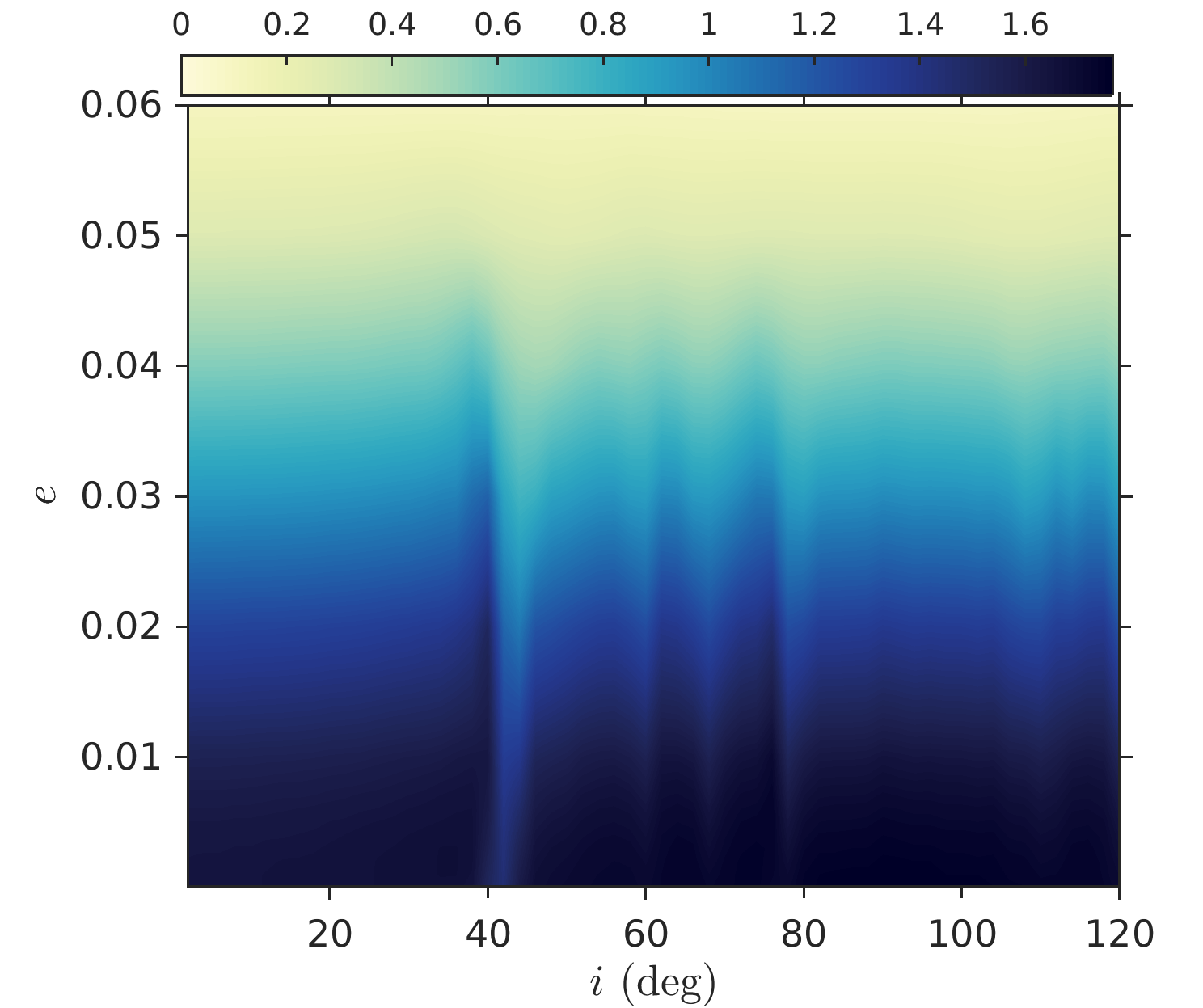
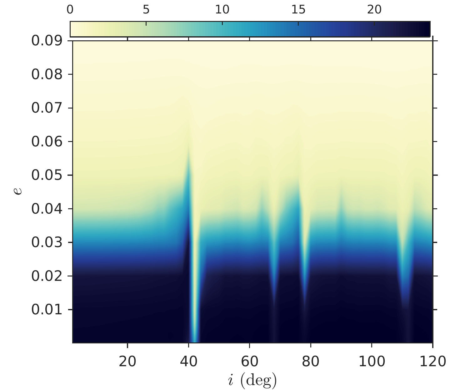
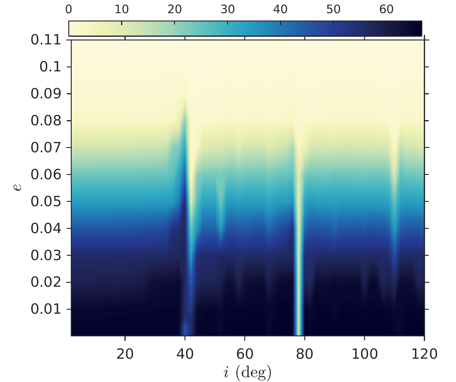
Figure 13: Lifetime computed over 120 years (color bar) as a function of initial inclination and eccentricity for $\Omega=180^{\circ}$ and $\omega=90^{\circ}$ at the initial epoch 2020, with $C_{R}(A/m)=1$ m${}^{2}/$kg. Left: $a=R_{E}+800$ km; middle: $a=R_{E}+1000$ km; right: $a=R_{E}+1200$ km.

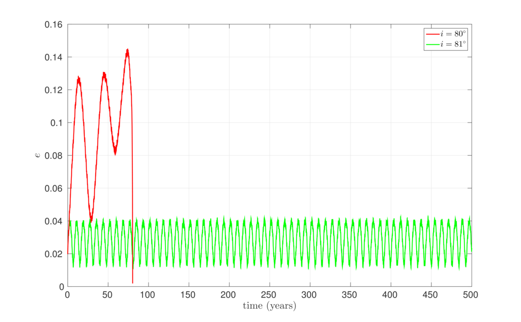
Figure 14: Eccentricity evolution considering $C_{R}(A/m)=1$ m${}^{2}/$kg, $a=R_{E}+1950$ km, $e=0.02$, $\Omega=270^{\circ}$, $\omega=270^{\circ}$ at the initial epoch 2020. The behavior computed starting from two neighboring values of inclination are shown: $i=80^{\circ}$ (red curve) which corresponds to a SRP resonance, and $i=81^{\circ}$ (green curve) which does not.

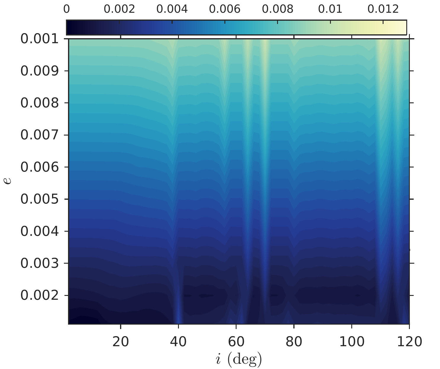
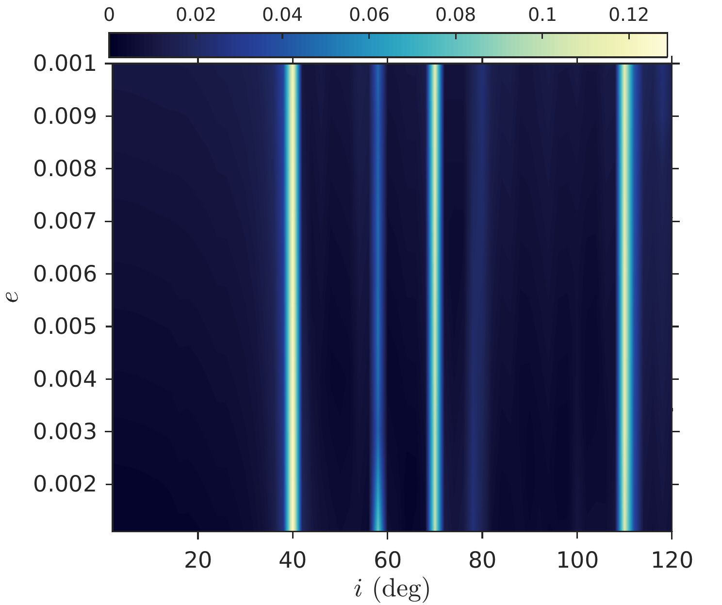
Figure 15: Maximum eccentricity computed over 120 years (color bar) for quasi-circular orbits as a function of initial inclination and eccentricity for $a=R_{E}+1560$ km, $\Omega=90^{\circ}$, $\omega=0^{\circ}$ at the initial epoch 2020. Left: $C_{R}(A/m)=0.024$ m${}^{2}/$kg; right: $C_{R}(A/m)=1$ m${}^{2}/$kg. Note the change of scale in the color bars between the left and the right panels.

The reader interested in different maps can find other cases in A2017a and A2017b .

3.3 On the Geopotential Expansion

Finally, we performed a sensitivity study in order to evaluate the role, in the dynamical evolution, of the terms of degree and order higher than 2 in the geopotential expansion. In Figure 16, we show the lifetime computed as a function of the initial $(\Omega,\omega)$ configuration considering at the initial epoch 2020 $a=7978.14$ km, $e=0.145$, $i=40^{\circ}$ and $i=56^{\circ}$, and three different dynamical models. In all cases, the dynamical model includes the atmospheric drag, SRP and lunisolar perturbations, but the geopotential is expanded up to degree and order 2, 3, and 5, respectively. Both $\Omega$ and $\omega$ are sampled at a step of 10^∘ in the range $[0^{\circ},360^{\circ})$. We show the outcome corresponding to a high value of initial eccentricity to emphasize the combined effect of one of the three perturbations with the atmospheric drag. The figure shows that a dynamical model which considers a geopotential expansion up to only degree and order 2, but even 3, does not depict accurately the dynamics and the long-term behavior in eccentricity, when this is induced to vary in a relative significant way by a given resonant perturbation.

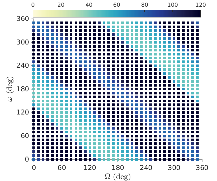
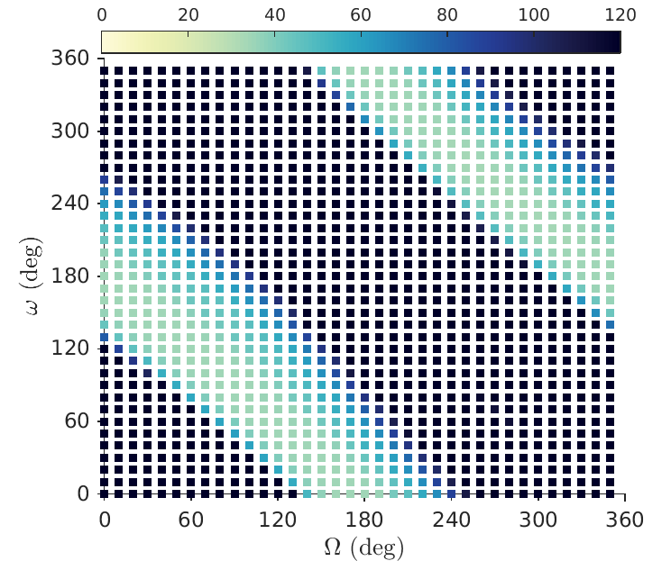
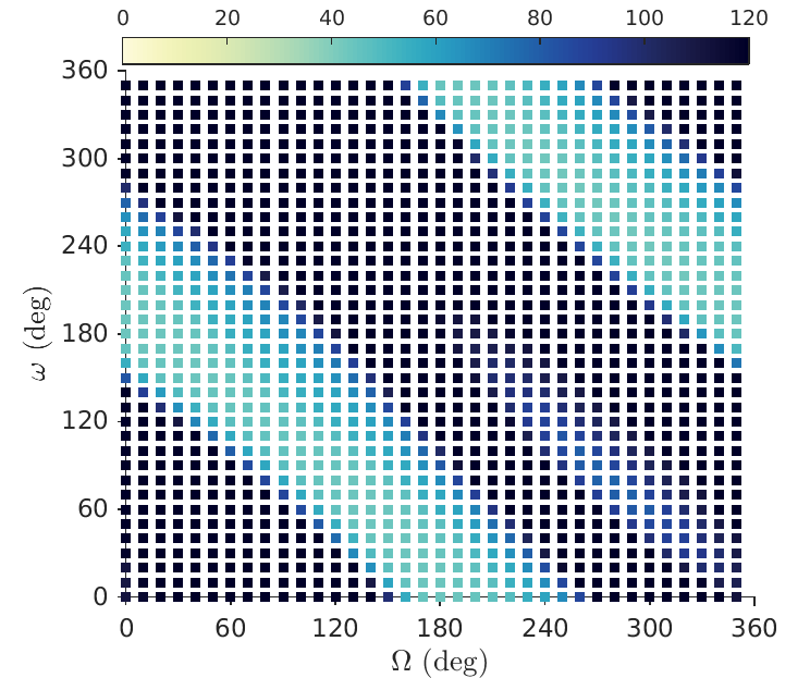
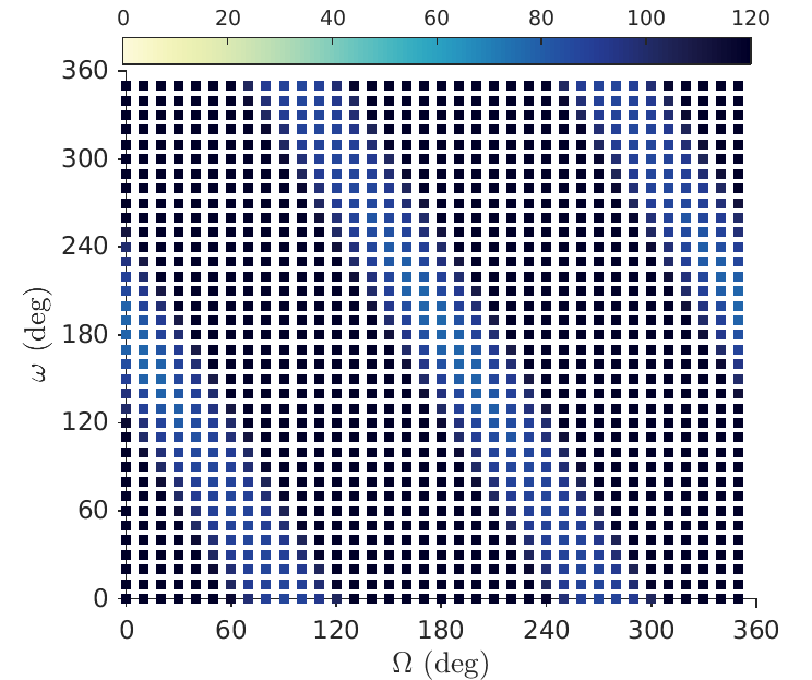
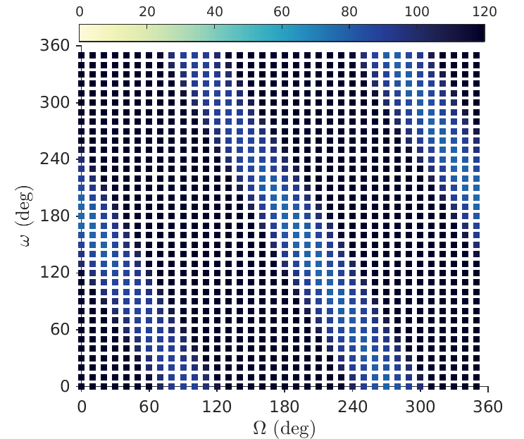
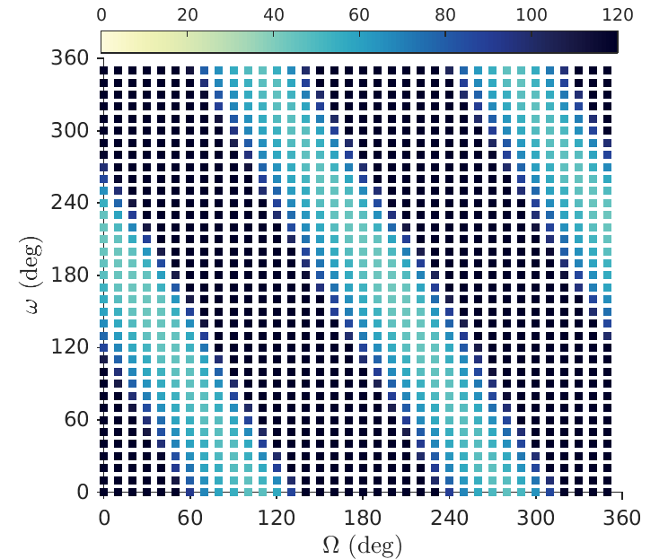
Figure 16: Lifetime computed as a function of the initial configuration $(\Omega,\omega)$, for $a=R_{E}+1600$km, initial $e=0.145$, epoch 2020, $C_{R}(A/m)=0.024\,$m${}^{2}/$kg. Top: initial inclination $i=40^{\circ}$. Bottom: initial inclination $i=56^{\circ}$. The different evolution due to the $2\times 2$ (left), $3\times 3$ (middle) or $5\times 5$ (right) geopotential in the dynamical model is compared.

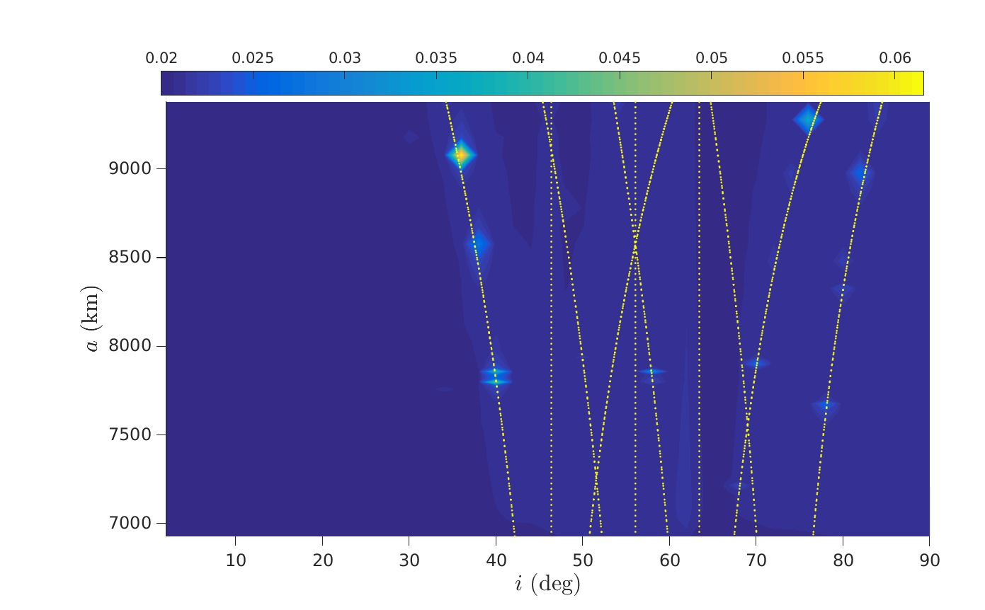
Figure 17: As a function of the initial inclination and semi-major axis, the maximum eccentricity value (color bar) computed in 120 years starting from $e=0.02$, $\Omega=0^{\circ}$, $\omega=0^{\circ}$. for the initial epoch 2018, considering $C_{R}(A/m)=0.012$ m²/kg and prograde orbits. The yellow lines denote the dominant resonances determining the long-term behavior. The yellow color of such lines does not mean that the corridors are always highly unstable.

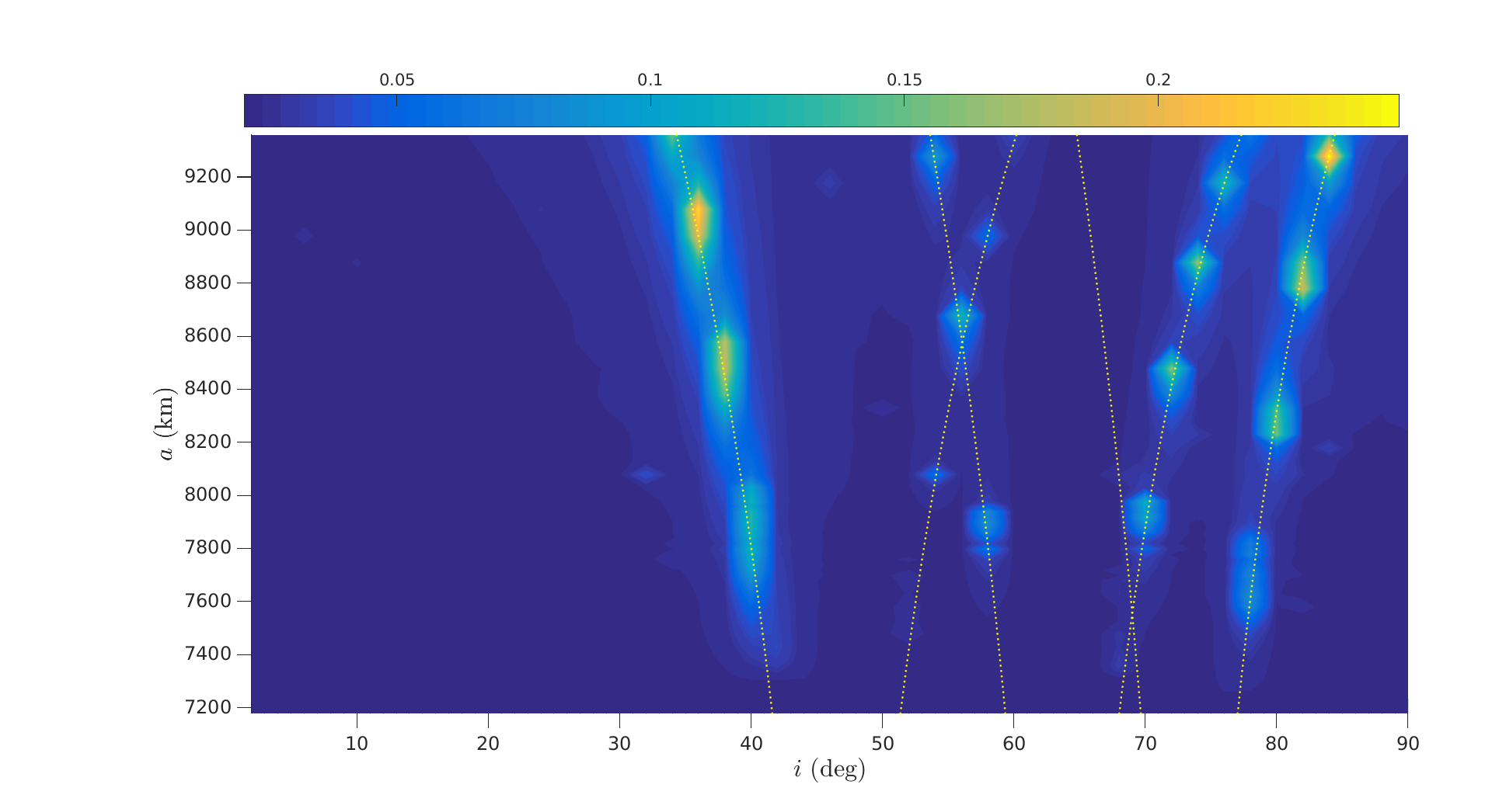
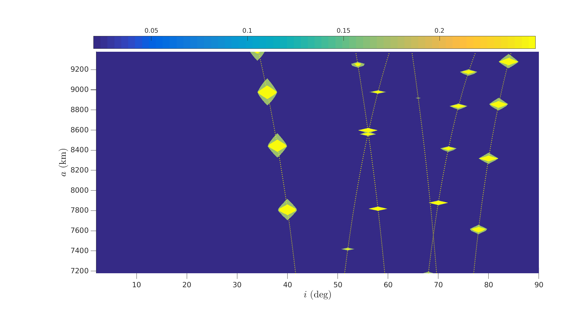
Figure 18: On the top, as a function of the initial inclination and semi-major axis, the maximum eccentricity value (color bar) computed in 120 years starting from $e=0.02$, $\Omega=0^{\circ}$, $\omega=0^{\circ}$. for the initial epoch 2020, considering $C_{R}A/m=1$ m²/kg and prograde orbits. On the bottom, the analytical estimate of the maximum variation in eccentricity is shown. The yellow lines denote the dominant resonances determining the long-term behavior. The yellow color of such lines does not mean that the corridors are always highly unstable.

4 Resonances in LEO

From a theoretical point of view, the simulations performed have allowed to recognize that the LEO region is permeated by a strong network of dynamical resonances, as recently highlighted also for the Medium Earth Orbit region (see, e.g., aR15 -A16 ). The main difference with respect to the previous studies on GNSS constellations is that in LEO the strongest advantage can be obtained not only from lunisolar resonances, but also from high-degree zonal harmonics and solar radiation pressure.

We recall that high-degree zonal harmonics, lunisolar perturbations, and solar radiation pressure cause long-term periodic variations in eccentricity, which become quasi-secular when a resonance involving the rate of $\Omega$ and $\omega$ occurs. In LEO, for the two values of area-to-mass ratio adopted, we can assume that $\omega$ and $\Omega$ vary only because of the oblateness of the Earth, and thus the corresponding rates depend only on $(a,e,i)$, that is,

$$\dot{\Omega}=-\frac{3}{2}\frac{J_{2}R^{2}_{E}n}{a^{2}(1-e^{2})^{2}}\cos i,\quad\quad\quad\dot{\omega}=\frac{3}{4}\frac{J_{2}R_{E}n}{a^{2}(1-e^{2})^{2}}\left(5\cos^{2}i-1\right),$$

being $J_{2}$ the second zonal term and $n$ the mean motion of the satellite (see, e.g., B ). This explains the inclination bands described in Section 3.2.

In Figure 17 and Figure 18 (top panel), we show, the maximum value, numerically computed, for the eccentricity in 120 years as a function of the initial inclination and semi-major axis, for prograde orbits starting from $e=0.02$, $\Omega=0^{\circ}$, $\omega=0^{\circ}$, $A/m=0.012$ m²/kg and $A/m=1$ m²/kg, respectively. In Figure 17, we show the locations of the following resonances:

• singly-averaged solar gravitational resonances (e.g., H80 )

  • $\dot{\psi}=2\dot{\omega}+\dot{\Omega}-2n_{S}\approx 0$,

  • $\dot{\psi}=2\dot{\omega}+2\dot{\Omega}-2n_{S}\approx 0$,

  where $n_{S}$ is the apparent mean motion of the Sun;

• doubly-averaged lunisolar gravitational perturbations (e.g., H80 )

  • $\dot{\psi}=\dot{\omega}\approx 0$,

  • $\dot{\psi}=2\dot{\omega}+\dot{\Omega}\approx 0$,

  • $\dot{\psi}=2\dot{\omega}+2\dot{\Omega}\approx 0$;

• $\dot{\psi}=\alpha\dot{\Omega}\pm\dot{\omega}\pm n_{S}\approx 0$, associated with SRP ($\alpha={0,1}$), gC62 -H77 .

For $A/m=1$ m${}^{2}/$kg, the only resonances which matter are the six resonances associated with SRP, namely those in the last bullet, which can be rewritten, for the sake of clarity as,

$$\dot{\psi}_{1} = \dot{\Omega}+\dot{\omega}-n_{S}\approx 0,$$

$$\dot{\psi}_{2} = \dot{\Omega}-\dot{\omega}-n_{S}\approx 0,$$

$$\dot{\psi}_{3} = \dot{\omega}-n_{S}\approx 0,$$

$$\dot{\psi}_{4} = \dot{\omega}+n_{S}\approx 0,$$

$$\dot{\psi}_{5} = \dot{\Omega}+\dot{\omega}+n_{S}\approx 0,$$

$$\dot{\psi}_{6} = \dot{\Omega}-\dot{\omega}+n_{S}\approx 0.$$

From Figure 18 (top), it is clear that, in this case, the variation in eccentricity that can be obtained at a resonance can definitely allow for a reentry. The amount of eccentricity increase can be estimated analytically in the following way. Let us assume that the instantaneous variation given by the Lagrange planetary equations can be written as

$$\frac{de}{dt}=A\sin{\psi},$$

where $A$ is a coefficient which depends on $(a,e,i)$, according to the given perturbation. By integration, we find that the detected variation in $e$ is proportional to $A$ and to the inverse of $\dot{\psi}$ A2018 . In Figure 18 (bottom), we show the variation in eccentricity computed in this way for the six SRP resonances, by assuming the same $(i,a)$ grid adopted for the numerical simulation. The color bar is bounded to the maximum value computed by propagation with FOP. Notice in particular the correspondence of the yellow islands between the two plots (top and bottom) in the figure. The effect of SRP resonances detected, especially in higher LEO and for $A/m=1$ m${}^{2}/$kg, is of paramount importance both from a theoretical and an applied point of view. Detailed theoretical findings obtained so far by our team can be found in A2018 and S2017 .

A remark to the long-term variation in eccentricity due to the zonal harmonic is in order. For the third harmonic $J_{3}$ it is given by:

$$\Delta e_{J_{3}}=-\frac{1}{2}\frac{J_{3}}{J_{2}}\frac{R_{E}}{a}\frac{e}{1-e^{2}}\sin i\sin\omega.$$

This is a classical result R , obtained by averaging the corresponding Lagrange planetary equation over the orbital period of the spacecraft, as well as over the period of the argument of pericenter. In an analogous way, it is possible to derive the long-term effect due to the fifth zonal harmonic. We have:

$$\Delta e_{J_{5}}=\frac{5}{128}\frac{J_{5}}{J_{2}}\left(\frac{R_{E}}{a}\right)^{3}\frac{\sin i}{(1-e^{2})^{2}(3+5\cos 2i)}\left[f(e,i)\sin\omega+g(e,i)\sin 3\omega\right].$$ (1)

for some specific $f,g$ functions (we omit the variation caused by $J_{4}$, because it varies with $\sin 2\omega$ without any special remark). It is worth noting, in particular, the singularity in the expression for $\Delta e_{J_{5}}$ in Eq. (1), occurring at $i\approx 63.4^{\circ}$ (and $i\approx 116.6$), which corresponds to the critical inclination where also $\dot{\omega}=0$. Notice that this result can be confirmed also averaging the expression of the effect in eccentricity due to $J_{5}$, given in M1961 .

It can be shown that the additional effect of the $J_{5}$ harmonics is significantly enhancing the perturbation in eccentricity with respect to the case where it is considered only $J_{3}$ or the lunisolar perturbations. An example of this behavior is shown in Figure 19, where different evolutions in time of the eccentricity and the pericenter altitude are depicted, depending on the contributions considered in the dynamical model (always assuming the effect of the atmospheric drag). In particular, the sharp decrease in lifetime is clear when zonal harmonic of degree 5 is included.

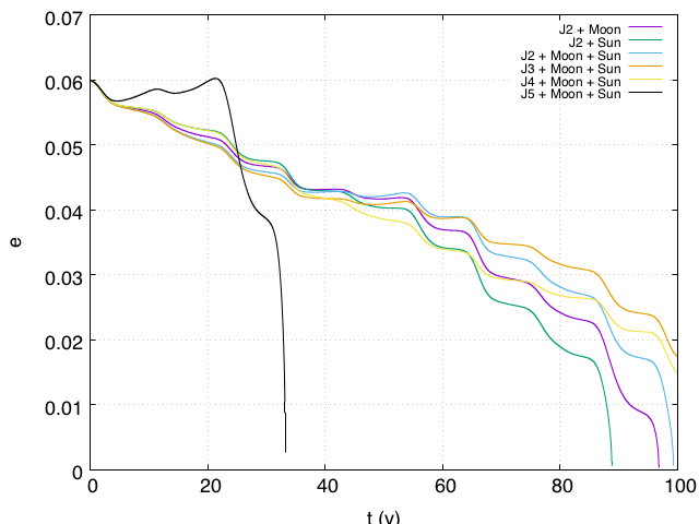
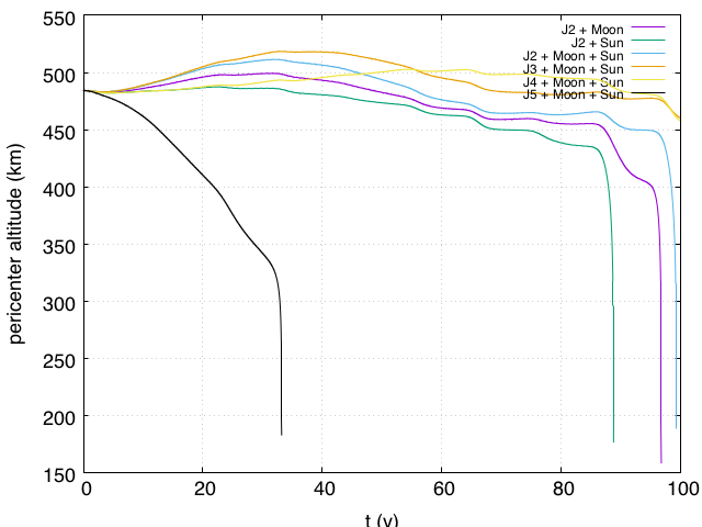
Figure 19: Comparison of the lifetime computed starting from the critical inclination $i=63.4^{\circ}$, considering different contribution in the dynamical model. For all the curves, the effect of the drag was included. What changes from one curve to the other is the maximum degree of the expansion in the geopotential and the lunisolar perturbations. Left: eccentricity behavior in time. Right: pericenter altitude behavior in time. Initial condition: $a=7300.14$ km, $e=0.06$, $\Omega=0^{\circ}$, $\omega=90^{\circ}$, epoch 2020, $C_{R}(A/m)=0.012$ m${}^{2}/$kg.

The identification of the principal resonances are fundamental not only to design natural deorbiting highways, but also to understand the characteristic period in the neighborhood of the quasi-secular eccentricity evolution. If an orbit is far from any resonance, the eccentricity evolves on a time-scale $\sim 2\pi/\dot{\omega}$, which depends solely on the geopotential. Close to a resonance, the eccentricity follows a longer secular time-scale, namely $\sim 2\pi/\dot{\psi}$, where $\psi$ is the critical angle of the dominant resonance. A detailed analysis on the characteristic frequencies detected for the eccentricity is under investigation.

5 Conclusions

We have shown the results obtained by mapping the LEO region from a dynamical perspective. The instability of a given orbit and the consequent lifetime change was evaluated as a function of the maximum value of eccentricity computed in 120 years. The whole mapping revealed that dynamical resonances can modify significantly the behavior in the long-term. For a typical value of area-to-mass ratio, this effect is quite mild, though in higher LEO solar radiation pressure effects can become important. The study paves the ways towards different challenges to be faced. Considering the design of affordable passive disposal solutions, we are now looking for the optimal strategy to enter into one of the resonant corridors to eventually achieve reentry. The focus will be put especially on the most populated regions in terms of semi-major axis and inclination. On the other hand, we are working in detail on the resonances found, in particular on the role of the initial phasing and on the regularity of the corresponding effects.

- (1) Alessi, E. M., Deleflie, F., Rosengren, A. J., Rossi, A., Valsecchi, G. B., Daquin, J., Merz, K., A Numerical Investigation on the Eccentricity Growth of GNSS Disposal Orbits, Celestial Mechanics and Dynamical Astronomy, 125, 71-90, (2016).
- (2) Alessi, E. M., Schettino, G., Rossi, A., Valsecchi, G. B., LEO Mapping for Passive Dynamical Disposal, Proceedings of the 7th European Conferences on Space Debris, Darmstadt, Germany, (2017).
- (3) Alessi, E. M., Schettino, G., Rossi, A., Valsecchi, G. B., Dynamical Mapping of the LEO Region for Passive Disposal Design, 68th International Astronautical Congress (2017), paper IAC-17.A6.2.7.
- (4) Alessi, E. M., Schettino, G., Rossi, A., Valsecchi, G. B., Solar radiation pressure resonances in Low Earth Orbits, Monthly Notices of the Royal Astronomical Society, 473, 2407–2414, (2018).
- (5) Anselmo, L., Cordelli, A., Farinella, P., Pardini C., Rossi, A., Study on long term evolution of Earth orbiting debris, ESA/ESOC contract No. 10034/92/D/IM(SC), (1996).
- (6) Battin, R. H., An Introduction to the Mathematics and Methods of Astrodynamics, Revised Edition, AIAA Education Series, American Institute of Aeronautics and Astronautics, Inc., Reston., (1999).
- (7) Breiter, S., Lunisolar Apsidal Resonances at Low Satellites Orbits, Celestial Mechanics and Dynamical Astronomy, 74, 253–274, (1999).
- (8) Breiter, S., Lunisolar Resonances Revisited, Celestial Mechanics and Dynamical Astronomy, 81, 81–91, (2001).
- (9) Celletti, A., Galeş, C., Dynamical investigation of minor resonances for space debris, Celestial Mechanics and Dynamical Astronomy, 123, 203 222, (2015).
- (10) Colombo, C., Letizia, F., Alessi, E. M., Landgraf, M., End-of-life Earth re-entry for highly elliptical orbits: the INTEGRAL mission, Proceedings of the AAS/AIAA Space Flight Mechanics Meeting, Santa Fe, New Mexico, AAS 14-156, (2014).
- (11) Colombo C., Gkolias, I., Analysis of orbit stability in the geosynchronous region for end-of-ife disposal, Proceedings of the 7th European Conference on Space Debris, Darmstadt, Germany, (2017).
- (12) Cook, G. E., Luni-solar perturbations of the orbit of an Earth satellite, The Geophysical Journal of the Royal Astronomical Society, 6, 271-291, (1962).
- (13) Ely, T. A., Howell, K. C., Dynamics of artificial satellite orbits with tesseral resonances including the effects of luni-solar perturbations, International Journal of Dynamics and Stability of Systems, vol. 12, 243 269, (1997).
- (14) ESA, ESA Space Debris Mitigation Compliance Verification Guidelines, ESSB-HB-U-002, (2015).
- (15) Frey, S., Lemmens, S., Status of the Space Environment: Current Level of Adherence to the Space Debris Mitigation Policy, Proceedings of the 7th European Conference on Space Debris, Darmstadt, Germany, (2017).
- (16) Frey, S., Private Communication, (2017).
- (17) Gkolias, I., Colombo, C., End-of-life disposal of geosynchronous satellites, 68th International Astronautical Congress, Adelaide, Australia, (2017), paper number IAC-17-A6.4.3.
- (18) Hughes, S., Satellite orbits perturbed by direct solar radiation pressure: general expansion of the disturbing function, Planetary and Space Science, 25, 809–815, (1977).
- (19) Hughes, S., Earth Satellite Orbits with Resonant Lunisolar Perturbations. I. Resonances Dependent Only on Inclination, Proceedings of the Royal Society of London. Series A, Mathematical and Physical Sciences, 372, 243–264, (1980).
- (20) Kwok, J. H., The long-term orbit prediction (LOP), JPL Technical Report EM 312/86-151, (1986).
- (21) Lamy, A., Morand, V., Le Fèvre, C., Fraysse, H., Resonance Effects on Lifetime of Low Earth Orbit Satellites, Proceedings of the 23rd International Symposium on Space Flight Dynamics, Pasadena, California, (2012).
- (22) Lewis, H.G., Radtke, J., Rossi, A., Beck, J., Oswald, M. Anderson, P. , Bastida Virgili, B., Krag, H., Sensitivity of the space debris environment to large constellations and small satellites, Proceedings of the 7th European Conferences on Space Debris, Darmstadt, Germany, (2017).
- (23) Liou, J.-C., Rossi, A, Krag, H., Raj, X. J., Anilkumar, A. K., Hanada, T., Lewis, H.G., Stability of the future LEO environment. Inter- Agency Space Debris Co-ordination Committee, AI 27.1 Report, IADC-12-08, (2013). available at http://www.iadc-online.org
- (24) Institute of Aerospace Systems, Technical University of Braunschweig, Meteoroid and Space Debris Terrestrial Environment Reference (MASTER-2009), ESA-SD-DVD-02, Release 1.0, December 2010 (updated in November 2012).
- (25) Merson, R. H., The Motion of a Satelilte in an Axi-symmetric Gravitational Field, Geophysical Journal, 4, 17–52, (1961).
- (26) Rosengren, A. J., Alessi, E. M., Rossi, A., Valsecchi, G. B., Chaos in navigation satellite orbits caused by the perturbed motion of the Moon, Monthly Notices of the Royal Astronomical Society, 449, 3522-3526, (2015).
- (27) Rossi, A., Anselmo, L., Pardini, C., Jehn, R., Valsecchi, G. B., The new space debris mitigation (SDM 4.0) long term evolution code, Proceedings of the 5th European Conference on Space Debris, Darmstadt, Germany, Paper ESA SP-672, (2009).
- (28) Rossi, A., Lewis, H., White, A., Anselmo, L., Pardini, C., Krag, H., Bastida Virgili, B., Analysis of the consequences of fragmentations in low and geostationary orbits, Advances in Space Research, 57, 1652–1663, (2016).
- (29) Rossi, A., and the ReDSHIFT team, The H2020 Project ReDSHIFT: Overview, First Results and Perspectives, Proceedings of the 7th European Conference on Space Debris, Darmstadt, Germany, (2017).
- (30) Roy, A. E., Orbital Motion, Institute of Physics Publishing, Bristol, (2005).
- (31) Schettino, G., Alessi, E. M., Rossi, A., Valsecchi G. B., Characterization of Low Earth Orbit dynamics by perturbation frequency analysis, 68th International Astronautical Congress, Adelaide, Australia, (2017), paper number IAC-17-C1.9.2.
- (32) Skoulidou, D. K., Rosengren, A. J., Tsiganis, K., Voyatzis, G., Long-term dynamics of artificial Earth satellites, Proceedings of the First Greek-Austrian Workshop on Extrasolar Planetary Systems, Ammouliani, Greece, (2016).
- (33) Skoulidou, D. K., Rosengren, A. J., Tsiganis, K., Voyatzis, G., Cartographic study of the MEO phase space for passive debris removal, Proceedings of the 7th European Conference on Space Debris, Darmstadt, Germany, (2017).
- (34) Urrutxua, H., Sanjurjo-Rivo, M., Paláez, J., DROMO propagator revisited, Celestial Mechanics and Dynamical Astronomy, 124, 1-31, (2016).