Intrinsic dimension and its application to association rules

Abstract

The curse of dimensionality in the realm of association rules is twofold. Firstly, we have the well known exponential increase in computational complexity with increasing item set size. Secondly, there is a related curse concerned with the distribution of (spare) data itself in high dimension. The former problem is often coped with by projection, i.e., feature selection, whereas the best known strategy for the latter is avoidance. This work summarizes the first attempt to provide a computationally feasible method for measuring the extent of dimension curse present in a data set with respect to a particular class machine of learning procedures. This recent development enables the application of various other methods from geometric analysis to be investigated and applied in machine learning procedures in the presence of high dimension.

1 Introduction

The curse of dimensionality in machine learning is a well known common place to flag the frontier to difficulty. However, in fact there are at least two peculiarities of this, i.e., the combinatorical explosion in high dimension and the (often) complicated data distribution in high dimension. Even though both are connected to some extent the latter is the object of investigation of this work, which we call from now on dimension curse. This effect is closely related to the mathematical phenomenon of concentration of measure, which was discovered by V. Milman [4] and is also known as the Lévy property. There are various works linking both worlds with the most comprehensive being [7, 6] by V. Pestov. His axiomatic approach led to a potent definition of intrinsic dimension, which is, however, computationally infeasible. Building up on his ideas we presented in [5] an applicable setup, which we summarize in the following. For this we recall crucial notions from [5] and show how data sets may be analyzed for dimension curse. We conclude our work with an exemplary application for association rules.

2 Observable Diameters and Dimension Function

Our approach for measuring the dimension curse for association rules is based on methods from geometric analysis. Hence, we need some mathematical structure that is accessible from both sides, geometrical methods as well as data representation. For this we developed the following 2.1 in [5]. But first, let us briefly recall some necessary basic mathematical notions. We call a topological space $X$ polish if $X$ is separable and there is a complete metric generating the topology of $X$. A set of functions $F\subseteq\mathbb{R}^{X}$ is called (pointwise) equicontinuous if $\forall x\in X,\varepsilon>0$ there exists a neighborhood $U$ of $x$ in $X$ with $\operatorname{diam}f(U)\leq\varepsilon$ for all $f\in F$. We utilize frequently the push-forward measure idea. Let $S,T$ be measurable spaces where $\mu$ is a measure on $S$ and $f:S\to T$ is a measurable map. The push-forward measure of $\mu$ is defined by $f_{*}(\mu)(B)\coloneqq\mu(f^{-1}(B))$ for every measurable set $B\subseteq T$. On a more technical note, for a measurable space $S$ with some measure $\mu$ and some measurable $T\subseteq S$ we denote by $\mu\!\!\upharpoonright_{T}$ the measure on the induced measure space $T$ defined by $(\mu\!\!\upharpoonright_{T})(B)\mathrel{\mathop{:}}=\mu(B)$ for every measurable $B\subseteq T$. Finally, for a finite non-empty set $S$ we denote by by $\nu_{S}$ the normalized counting measure on $S$.

Definition 2.1 (Data Structure [5]).

A data structure is a triple ${D=(X,\mu,F)}$ consisting of a Polish space $X$ together with a Borel probability measure $\mu$ on $X$ and an equicontinuous set $F$ of real-valued functions on $X$, where the elements of $F$ will be referred to as the features of $D$. We call $D_{\mathrm{triv}}\mathrel{\mathop{:}}=(\{\emptyset\},\nu_{\{\emptyset\}},\mathbb{R})$ the trivial data structure. Given a data structure $D=(X,\mu,F)$, we let

$$\widehat{D}\,\mathrel{\mathop{:}}=\left.\left(X,\mu,F\cup\left\{f\in\mathbb{R}^{X}\right|f\text{ constant}\right\}\right).$$

We call two data structures $D_{i}=(X_{i},\mu_{i},F_{i})$ $(i\in\{0,1\})$ isomorphic and write $D_{0}\cong D_{1}$ if there exists a homeomorphism $\varphi\colon\operatorname{spt}\mu_{0}\to\operatorname{spt}\mu_{1}$ such that $\varphi_{\ast}\!\left(\mu_{0}\!\!\upharpoonright_{\operatorname{spt}\mu_{0}}\right)=\mu_{1}\!\!\upharpoonright_{\operatorname{spt}\mu_{1}}$ and $(F_{1}|_{\operatorname{spt}\mu_{1}})\circ\varphi=F_{0}|_{\operatorname{spt}\mu_{0}}$.

In [5] we elaborated on this definition. In particular, we introduced a pseudo metric on the collection of all data structures, a variant of Gromov’s observable distance [3, Chapter 3$\tfrac{1}{2}$.H]. We utilize this as a tool for analyzing high dimensional data, as proposed by Pestov [7, 6]. However, we will refrain to introduce the specifics of this pseudo metric and refer to it informally for the rest of this work.

The goal now is to find a mathematical sound dimension function for the collection of all data structures. We may skip the necessary propositions and proceeding mathematical notions and state the two most important properties to expect from a dimension function informally. First, a dimension function should reflect the presence of the concentration phenomenon in a data structure. More precisely, a dimension function shall diverge on a sequence of data structures if and only if this sequence has the Lévy property. Second, if a sequence of data structures concentrates (w.r.t. the pseudo metric) to a particular data structure, the dimension function shall concentrate to its value on this data structure as well. For the further complete axiomatization we refer the reader to [5].

For reasons of space, we may not address the various technical mathematical challenges, preparations and connections to geometric analysis. We rather jump to the main result of [5], a new quantity for expressing the extent to which a data structure is prone to the dimension curse: the intrinsic dimension. For this we adapt further the ideas from [3, Chapter 3$\tfrac{1}{2}$] about observable diameters.

Definition 2.2 (Observable Diameter [5]).

Let $\alpha\geq 0$. We call Equation 1 the $\alpha$-partial diameter of a Borel probability measure $\nu$ on $\mathbb{R}$ and we call Equation 2 the $\alpha$-observable diameter of a data structure $D=(X,\mu,F)$.

$$\mathrm{PartDiam}(\nu,1-\alpha)\mathrel{\mathop{:}}=\inf\{\operatorname{diam}(B)\mid B\subseteq\mathbb{R}\text{ Borel},\,\nu(B)\geq 1-\alpha\}$$ (1)

$$\mathrm{ObsDiam}(D;-\alpha)\mathrel{\mathop{:}}=\sup\{\mathrm{PartDiam}(f_{\ast}(\mu),1-\alpha)\mid f\in F\}$$ (2)

We showed in [5] that the observable diameter is invariant under isomorphisms of data structures and it fulfills a continuity property with respect to the earlier mentioned pseudo metric. Building up on this definition we can state: The map $\partial_{\Delta}\colon\mathcal{D}\to[1,\infty]$ defined by Equation 3 is a dimension function.

$$\partial_{\Delta}(D)\mathrel{\mathop{:}}=\frac{1}{\left(\int_{0}^{1}\mathrm{ObsDiam}(D;-\alpha)\wedge 1\,\mathrm{d}\alpha\right)^{2}}\qquad(D\in\mathcal{D})$$ (3)

3 Example Experiment and Applications

Distance functions, as often used in machine learning procedures, are a natural candidate for feature functions. Hence, we might not need to motivate the applicability of the intrinsic dimension for those. However, the idea of dimension function in mathematical data structures is able to cope with any kind of proper feature function set. Therefore we decided for an exemplary application in association rule mining. A possible adaption of data structures and observable diameter could be done as follows: We consider a set – we restrict our example to non repeating transactions – of transactions $T=\{t_{1},\dotsc,t_{m}\}$ with transactions $t_{i}\subseteq I$ where $I=\{i_{1},\dotsc,i_{n}\}$ is called itemset. An assocation rule on $I$ then is an element $(X,Y)\in\mathcal{P}(I)\times\mathcal{P}(I)$ such that $X\cap Y=\emptyset$ and $\forall t\in T:X\subseteq t\Rightarrow Y\subseteq t$. We denote by $R$ the set of all association rules for $T$, and by $X^{T}$ the subset $S\subseteq T$ such that $\forall t\in S:X\subseteq t$. To convert this data into a mathematical data structure like introduced in 2.1 we take the following approach: $D=(T,\nu_{T},F(T))$ with $F(T)\coloneqq\{\nu_{I}(Y)\cdot\mathds{1}_{X^{T}}\mid(X,Y)\in R\}$. Hence, we consider the transactions as data points and the feature functions are mappings from those data points to the support of a head of a rule, i.e., the relative amount of items covered by this particular rule. Using this setup the $\mathrm{PartDiam}(\nu_{I}(Y)\cdot\mathds{1}_{X^{T}},1-\alpha)=\nu_{I}(Y)$ if $\alpha<\nu_{T}(X^{T})<1-\alpha$ and $0$ otherwise, for all rules $(X,Y)\in R$. Hence, this yields $\mathrm{ObsDiam}(D,-\alpha)=\sup\{\nu_{I}(Y)\mid(X,Y)\in R,\alpha<\nu_{T}(X^{T})<1-\alpha\}$. We plotted in Figure 1 multiple example calculations for well known association rule minining data sets, i.e., accident [2], mushroom and chess [1]. We observe an increase in dimension with the increase of support.

This is expected due to the antitone character of feature sets. However, the slope differs among the different data sets and confidence values, revealing the ability of the particular feature sets to cover the data.

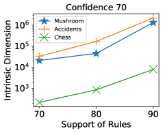
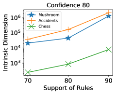
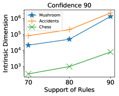
Figure 1: The intrinsic dimension for multiple data sets, supports and confidence.

3.0.1 Conclusion

We presented in this work an mathematical approach for measuring the dimension curse in machine learning. The novelty here is the computationally feasible character. Besides the indicated application for association rules there are various applications possible, and from the standpoint of understanding the dimension curse, necessary. One particular crucial application could be assessing the results of dimension reduction procedures like Principle Component Analysis.

Acknowledgments
F.M.S. acknowledges funding of the Excellence Initiative by the German Federal and State Governments, as well as the Brazilian CNPq, processo 150929/2017-0.

References

- [1] D. Dheeru and E. K. Taniskidou “UCI Machine Learning Repository”, 2017 URL: http://archive.ics.uci.edu/ml
- [2] K. Geurts, G. Wets, T. Brijs and K. Vanhoof “Profiling High Frequency Accident Locations Using Association Rules” In Proceedings of the 82nd Annual Transportation Research Board, Washington DC. (USA), January 12-16, 2003, pp. 18
- [3] M. Gromov “Metric structures for Riemannian and non-Riemannian spaces. Transl. from the French by Sean Michael Bates. With appendices by M. Katz, P. Pansu, and S. Semmes. Edited by J. LaFontaine and P. Pansu.” Boston, MA: Birkhäuser, 1999, pp. xix + 585
- [4] M. Gromov and V. D. Milman “A Topological Application of the Isoperimetric Inequality” In American Journal of Mathematics 105.4 Johns Hopkins University Press, 1983, pp. 843 URL: http://www.jstor.org/stable/2374298
- [5] T. Hanika, F. M. Schneider and G. Stumme “Intrinsic dimension of concept lattices” In CoRR abs/1801.07985, 2018 arXiv: http://arxiv.org/abs/1801.07985
- [6] V. Pestov “An axiomatic approach to intrinsic dimension of a dataset” In Neural Networks 21.2-3, 2008, pp. 204–213 DOI: 10.1016/j.neunet.2007.12.030
- [7] V. Pestov “Intrinsic dimension of a dataset: what properties does one expect?” In Proceedings of the International Joint Conference on Neural Networks, IJCNN 2007, Celebrating 20 years of neural networks, Orlando, Florida, USA, August 12-17, 2007, 2007, pp. 2959–2964 DOI: 10.1109/IJCNN.2007.4371431