Optimal operating protocol to achieve efficiency at maximum power of heat engines

Abstract

The efficiency at maximum power has been investigated extensively, yet the practical control scheme to achieve it remains elusive. We fill such gap with a stepwise Carnot-like cycle, which consists the discrete isothermal process (DIP) and adiabatic process. With DIP, we validate the widely adopted assumption of $\mathscr{C}/t$ relation of the irreversible entropy generation $S^{(\mathrm{ir})}$, and show the explicit dependence of the coefficient $\mathscr{C}$ on the fluctuation of the speed of tuning energy levels as well as the microscopic coupling constants to the heat baths. Such dependence allows to control the irreversible entropy generation by choosing specific control schemes. We further demonstrate the achievable efficiency at maximum power and the corresponding control scheme with the simple two-level system. Our current work opens new avenues for the experimental test, which was not feasible due to the lack the of the practical control scheme in the previous low-dissipation model or its equivalents.

I Introduction

Designing optimal heat engine is one of the primary goals in the recent flourishing studies of heat engines both classically CA-endoreversible-heat-engine ; actual-heat-engine ; endoreversible-HEs ; Linear-irreversible-heat-engine ; Linear-irreversible-HE-1 and quantum mechanically density-matrix-expansion-1 ; quantun ; TLA-heat-engine . One of the most important characteristics is the output power, which measures the energy output per unit of time. When the output power achieves its maximum value, the corresponding efficiency, known as efficiency at maximum power (EMP) EMP0 ; EMP1 ; EMP2 ; EMP-Tu ; EMP3 ; constriant2-1 ; constriant2 , is another important characteristic of the heat engine. The achievable EMP is well investigated via low-dissipation model low-dissipation , which is recently proved to be equivalent to the linear response model Linear-irreversible-low-disspation . The low-dissipation model simply assumes that the irreversible entropy generation, characterizing the irreversibility, is inversely proportional to the operation time $t$ with a coefficient $\mathscr{C}$, namely $\mathscr{C}/t$ relation. The EMP is achieved via optimizing the operation times, as well as the coefficients. However, such simple model leaves two major questions: (1) how universal is the $\mathscr{C}/t$ relation? and (2) what is the control protocol to achieve the corresponding EMP? The second question is critical to the engine design, as well as the experimental test.

The main obstacle to answer the two underline questions is the lack of a microscopic model, with which the operating cycle can be shown explicitly, and kept simple enough to allow analytically proof. To maintain efficiency, it is meaningful to follow the Carnot cycle, which consists two isothermal processes and two adiabatic processes. The main difficulty is to design a quasi-isothermal process, which refers to a process with finite operation time while in contact with a heat bath. We have initialized such attempt to overcome the difficulty in our previous work TLA-heat-engine , yet limited to two-level system with a simple linear tuning of energy levels.

In the current paper, we design a discrete isothermal process, which consists a series of quantum isochoric and quantum adiabatic sub-processes. With such discrete process, the $\mathscr{C}/t$ relation is analytically validated in the low-dissipation region for arbitrary finite-dimension system under arbitrary control scheme. Moreover, we obtain for the first time the exact dependence of coefficient $\mathscr{C}$ on a few parameters of the control scheme in the discrete isothermal process. Based on this discovery, we design a two-level stepwise Carnot-like heat engine and tune energy levels in different ways when it contacts with the high temperature and low temperature heat bath. As a result, the EMP of such heat engine is found to be controllable, and in some circumstances, can be effectively improved.

II Irreversible entropy generation in discrete isothermal process

In this section, we will construct a discrete process operating under finite time to resemble the isothermal process in Carnot cycle and prove the $\mathscr{C}/t$ relation. The Carnot efficiency, $\eta_{C}=1-T_{C}/T_{H}$, is the fundamental upper bound, which a heat engine working between two heat baths with temperatures $T_{H}$ and $T_{C}$ can achieve Carnot . Naturally, it is straightforward to design Carnot-like process to achieve maximum efficiency under given output power. The key question is how to realize a finite-time operation resembling isothermal process, which usually takes infinite time in Carnot cycle.

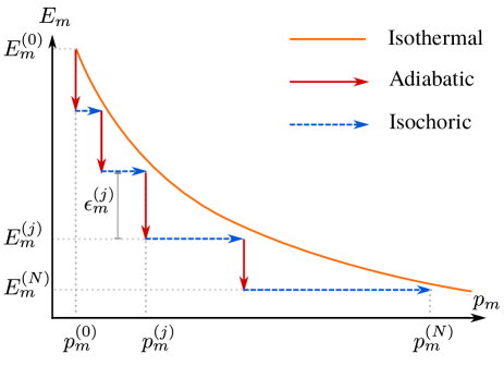
Figure 1: (Color online) Schematic illustration of a discrete isothermal process (DIP). The horizontal axis in this figure is the occupation probability of the system in its $m$-th energy level, while the vertical axis indicates the eigenenergy of the $i$th energy level of the system. The solid orange curve represents the isothermal process, which follows $p_{m}=e^{-\beta E_{m}}/\sum_{m}e^{-\beta E_{m}}$. The red vertical lines and the blue horizontal dashed lines represent the quantum adiabatic and quantum isochoric processes, respectively.

The isothermal process is an ideal process based on the quasi-static assumption that the changing speed of the system’s energy levels is far slower than the relaxation of the system contacting with the heat bath, so that the system is constantly on the thermal equilibrium state with the same temperature of the heat bath. However, in the finite time quasi-isothermal process, the system deviates from the thermal equilibrium state. In our model, we consider the finite-time process, where the system is not necessary in thermal equilibrium for all the time.

The system of interest, initially in the thermal equilibrium state with inverse temperature $\beta=(k_{B}T)^{-1}$, has $M$ discrete energy levels $\{E_{m}^{(0)}\}$ ($m=1,2...,M$). And the corresponding occupation probabilities in these energy levels are $\{p_{m}^{(0)}\}$ with $p_{m}^{(0)}=e^{-\beta E_{m}^{(0)}}/\sum_{m}e^{-\beta E_{m}^{(0)}}$. To approach the quasi-isothermal process, we introduce the discrete isothermal process (DIP) discrete-isothermal-process ; DIP , which includes a series of quantum adiabatic processes and quantum isochoric processes QIP1 ; QIP2 .

As illustrated in Fig. 1, the ideal isothermal process (orange solid curve) is decomposed by a series of $N$ alternating short quantum adiabatic processes (red solid lines) and quantum isochoric processes (blue dashed lines). One big difference from the ideal isothermal process is that the discrete quasi-isothemal process is operated within a finite duration $t_{f}$. We assume the $j-$th sub quantum isochoric process takes time $\tau_{j}$ ($j=1,2,\dots,N$), while each sub quantum adiabatic process is operated by a sudden quench with no time cost. We assume that all the instantaneous eigen levels $E_{m}$ are always avoided level-crossing. Therefore, even though the adiabatic process is quenched, the instantaneous eigen states keep unchanged and the quantum adiabatic condition is satisfied QIP2 ; Messiah_adiabatic .

The operation time of the $j-$th step $\tau_{j}$ can not be infinitesimal due to the requirement of the thermalization process. Detailed discussion about the time scale of the step time will appear later. Through the whole quasi-isothermal process, the energy spectra of the system are changed from $\{E_{m}^{(0)}\}$ to $\{E_{m}^{(N)}\}$, while the corresponding occupation probabilities turn from $\{p_{m}^{(0)}\}$ to $\{p_{m}^{(N)}\}$. In the $j$-th subprocess, the $m$-th energy level is pulled from $E_{m}^{(j-1)}$ to $E_{m}^{(j)}=E_{m}^{(j-1)}+\epsilon{}_{m}^{(j)}$ in the quantum adiabatic process (the occupation possibility is not changed in this process). The tuning scheme of the energy levels $\{\epsilon_{m}^{(j)}\}$ can be described by a control function $f_{m}(j)=\sum_{k=1}^{j}\epsilon{}_{m}^{(k)}$, with constraints $f_{m}(N)=E_{m}^{(N)}-E_{m}^{(0)}\equiv\Delta_{m}$ and $f_{m}\left(0\right)=0$. And the time to reach the $j-th$ step is $t_{j}=\sum_{k=1}^{j}\tau_{k}$. Each sub quantum adiabatic process is followed by a sub quantum isochoric process, during which the corresponding occupation possibility is changed from $p_{m}^{(j-1)}$ to $p_{m}^{(j)}$ without shifting energy levels. The occupation possibility then is assumed to relax to the corresponding equilibrium state with probability

$$p_{m}^{(j)}=\frac{e^{-\beta E_{m}^{(j)}}}{\sum_{m=1}^{M}e^{-\beta E_{m}^{(j)}}},$$ (1)

noticing the step time $\tau_{j}$ should be far larger than the typical relaxation time of the heat bath to fulfill the low-dissipation condition. The deviation from the equilibrium state is explicitly evaluated in the Appendix A with an example of two-level atom. In the $j$-th subprocess, there is no heat exchange between the system and bath in adiabatic process, so the heat transfer only appears in the isochoric process QIP2 ; heat-and-work with $\Delta Q^{(j)}=\sum_{m=1}^{M}E_{m}^{(j)}\delta p_{m}^{(j)}$ , where $\delta p_{m}^{(j)}\equiv p_{m}^{(j)}-p_{m}^{(j-1)}$. Thus, the heat transfer in the whole process $\Delta Q=\sum_{j=1}^{N}\Delta Q^{(j)}$ can be explicitly written as

$$\Delta Q=\sum_{j=1}^{N}\sum_{m=1}^{M}[E_{m}^{(0)}+\sum_{k=1}^{j}\epsilon_{m}^{(k)}]\delta p_{m}^{(j)}.$$ (2)

In the high temperature limit $\beta E_{m}\ll 1$, by keeping the first order of $\beta E_{m}$, the above equation is simplified as

$$\Delta Q=\sum_{j=1}^{N}\sum_{m=1}^{M}[-\frac{\beta}{M}\epsilon_{m}^{(j)}+\frac{\beta}{M^{2}}\sum_{m=1}^{M}\epsilon_{m}^{(j)}][E_{m}^{(0)}+\sum_{k=1}^{j}\epsilon{}_{m}^{(k)}].$$ (3)

On the other hand, the change in Shannon entropy $S=-\sum_{m=1}^{M}p_{m}\ln p_{m}$ ($k_{B}=1$) only depends on the initial and final state of the system, namely,

$$\Delta S =S^{(N)}-S^{(0)}$$

$$=-\frac{\beta^{2}\sum_{m=1}^{M}(E_{m}^{(N)})^{2}}{M}+\frac{\beta^{2}(\sum_{m=1}^{M}E_{m}^{(N)})^{2}}{2M^{2}}$$

$$+\frac{\beta^{2}\sum_{m=1}^{M}(E_{m}^{(0)})^{2}}{M}-\frac{\beta^{2}(\sum_{m=1}^{M}E_{m}^{(0)})^{2}}{2M^{2}}.$$ (4)

With the heat exchange in Eq. (4) and the entropy change in Eq. (3), we obtain the irreversible entropy generation $S^{(\mathrm{ir})}=\Delta S-\Delta Q/T$ as

$$S^{(\mathrm{ir})}=\frac{\beta^{2}}{2M}\sum_{j=1}^{N}\left[\sum_{m=1}^{M}(\epsilon_{m}^{(j)})^{2}-\frac{1}{M}(\sum_{m=1}^{M}\epsilon_{m}^{(j)})^{2}\right].$$ (5)

For simplicity, we consider the case that the operation time of each subprocess is the same, namely, $\tau_{j}=\tau$. And the total operation time is $t_{f}=N\tau$. Then, by introducing the average tuning speed of each step $v_{m}^{(j)}\equiv\epsilon_{m}^{(j)}/\tau$, we simplify Eq. (5) as

$$S^{(\mathrm{ir})}=\frac{\beta^{2}\overline{\Delta}^{2}}{2(t_{f}/\tau)}\frac{\left\langle\overline{v^{2}}\right\rangle-\left\langle\overline{v}^{2}\right\rangle}{\left\langle\overline{v}\right\rangle^{2}},$$ (6)

where

$$\left\langle\overline{v}\right\rangle\equiv\frac{1}{N}\sum_{j=1}^{N}[\frac{1}{M}\sum_{m=1}^{M}v_{m}^{(j)}],$$ (7a)

$$\left\langle\overline{v^{2}}\right\rangle\equiv\frac{1}{N}\sum_{j=1}^{N}[\frac{1}{M}\sum_{m=1}^{M}\left(v_{m}^{(j)}\right)^{2}],$$ (7b)

$$\left\langle\overline{v}^{2}\right\rangle\equiv\frac{1}{N}\sum_{j=1}^{N}\left(\frac{1}{M}\sum_{m=1}^{M}v_{m}^{(j)}\right)^{2}.$$ (7c)

Here $\overline{\bullet}$ means the average over the energy levels, while $\left\langle\bullet\right\rangle$ means the average over the whole process. $\overline{\Delta}=\sum_{m=1}^{M}\Delta_{m}/M$ is the average energy difference of the system’s energy levels. Eq. (6) is the main result of this paper, and its importance lies in two aspects. Firstly, Eq. (6) shows that the irreversible entropy generation follows the $\mathscr{C}/t$ relation.With the current result, we basically answer the first question posted in the introduction.

Secondly, the result in Eq. (6) shows the explicit dependence of the coefficient $\mathscr{C}$ on the control scheme via the fluctuation of tuning speed. To further decouple the system constants and the control scheme, we define

$$\Theta\equiv\frac{\beta^{2}\overline{\Delta}^{2}}{2},\xi\equiv\frac{\left\langle\overline{v^{2}}\right\rangle-\left\langle\overline{v}^{2}\right\rangle}{\left\langle\overline{v}\right\rangle^{2}},$$ (8)

and rewrite the irreversible entropy generation as

$$S^{(\mathrm{ir})}=\frac{\Theta\xi}{t_{f}/\tau}.$$ (9)

Here, $\Theta$ is related to the starting and ending point of the stepwise isothermal process, $\xi$ shows the impact of different control scheme. The coefficient is $\mathscr{C}=\Theta\xi\tau$. The above relation clearly shows that the irreversible entropy generation $S^{(ir)}\rightarrow 0$ in the limit $t_{f}\rightarrow\infty$($N\rightarrow\infty$), which is consistent with the Quasi-static isothermal process.

When we consider the total operation time of the discrete isothermal process (DIP), we have two adjustable parameters, namely the step operation time $\tau$ and the total step number $N$. So the total operation time $t_{f}$ can also be increased by increasing the step time $\tau$. However, the irreversible entropy generation $S^{(ir)}$ approaches a fixed non-zero value, when increase the total operation time $t_{f}$ via increasing the step time $\tau$ with fixed step number $N$. In such case, the DIP will not back to the isothermal process, and thus the requirement of recovering the Carnot cycle in the limit $t_{f}\rightarrow\infty$ will not be fulfilled. Therefore, in our derivation, we fix the step time and choose the total step number $N$ to be the adjustable parameter.

$f(k)$	$\xi$	$S^{(\mathrm{ir})}$
$ak^{n}$	$\frac{n^{2}}{2n-1}$	$\frac{n^{2}}{2n-1}\frac{\beta^{2}\Delta^{2}}{8N}$
$b\left(\textrm{e}^{ak}-1\right)$	$\left(\frac{1}{2}+\frac{b}{\Delta}\right)\ln(\frac{\Delta}{b}+1)$	$\left(\frac{1}{2}+\frac{b}{\Delta}\right)\ln(\frac{\Delta}{b}+1)\frac{\beta^{2}\Delta^{2}}{8N}$
$a\ln\left(bk+1\right)$	$\frac{\sinh^{2}\left(\Delta/2a\right)}{\left(\Delta/2a\right)^{2}}$	$\frac{\sinh^{2}\left(\Delta/2a\right)}{\left(\Delta/2a\right)^{2}}\frac{\beta^{2}\Delta^{2}}{8N}$

Table 1: Irreversible entropy generation of different typical control functions for the case of two-level atom. Here, each function satisfies the constraint $f(0)=0$ and $f(N)=\Delta$, where $\Delta$ is the energy level change during the DIP. In the calculation, we have already assumed that $N\gg 1$

In the case of the two-level system ($M=2$), whose ground state energy $E_{1}$ is taken as 0 in the whole process, Eq. (6) reduces to

$$S^{(\mathrm{ir})}=\frac{\beta^{2}\Delta^{2}}{8t_{f}/\tau}\frac{\left\langle v^{2}\right\rangle}{\left\langle v\right\rangle^{2}},$$ (10)

where $\left\langle v\right\rangle=\sum_{j=1}^{N}v_{2}^{(j)}/N$ and $\left\langle v^{2}\right\rangle=\sum_{j=1}^{N}\left(v_{2}^{(j)}\right)^{2}/N$ are the average of tuning speed and average of the square of tuning speed, respectively. $\Delta=E_{2}^{(N)}-E_{2}^{(0)}$ is the energy change of the excited state of the two-level system. When the energy level control function $f(k)$ is linear dependent on the step, $\xi$ reaches the minimal value 1, in which case the the irreversible entropy generation takes the minimal value, namely, $S^{(ir)}=\beta^{2}\Delta^{2}/(8t_{f}/\tau).$ This result shows that the irreversible behavior of the system can be effectively reduced by optimizing the control protocol of the system’s energy levels in the DIP. A similar idea was reported in the optimization of quantum Otto heat engine super-adibatic , where the authors introduced the super-adiabatic process to achieve zero friction in the thermodynamic cycle. To make sure the system is at thermal equilibrium in the end of each subprocess, the step time $\tau$ should be larger than the relaxation time $1/\widetilde{\gamma}$, namely, $\tau>1/\widetilde{\gamma}$. Here, $\widetilde{\gamma}=2\gamma/\left(\beta E^{(0)}\right)$ is obtained in the high temperature limit (see Appendix A), and $\gamma$ is the system-bath coupling constant. For the nonlinear control functions of time, i.e. $\xi>1$, the corresponding irreversible entropy generation is larger than that of the linear case.

In Table. 1, we demonstrate the exact expressions of the irreversible entropy generation related to three typical control functions with the two-level atom example. When the control function is taken as power function, i.e., $f(k)\propto k{}^{n}$, the irreversible entropy generation follows a simple relation as $S_{n}^{(\mathrm{ir})}=n^{2}S_{1}^{(\mathrm{ir})}/(2n-1)$, where $S_{1}^{(\mathrm{ir})}=\beta^{2}\Delta^{2}/(8t_{f}/\tau)$. This relation is confirmed by the master equation based numerical results (the points) as illustrated in Fig. 2, where we plot the irreversible entropy generation as a function of operation time with $N=t_{f}/\tau\in[20,120]$. In the simulation, we fix the step time with $\tau=1$ and increase the number of steps $N$. The initial energy of excited state is $E_{2}^{\left(0\right)}=10$ and the final one is $E_{2}^{\left(N\right)}=6$. The inverse temperature is $\beta=0.1$, and the decay rate is $\gamma=1$. The adiabatic process is assumed to be instantaneous. During the isochoric process, the evolution of the system is govern by the master equation as shown in Eq. (18). With the increase of $n$ of the control function $f(k)$, the irreversible entropy generation is also increased as illustrated in Fig. 2. The numerical results are in good agreement with theoretical prediction in Eq. (10).

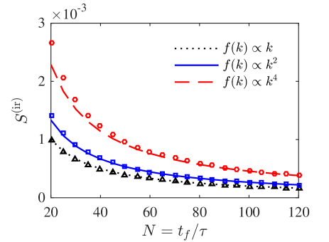
Figure 2: (Color online) Irreversible entropy generation as function of operation time, where $f(k)=\Delta(k/N)$ (black), $f(k)=\Delta(k/N)^{2}$ (blue), and $f(k)=\Delta(k/N)^{4}$ (red). The points represent the numerical results, and the lines represent the analytical results of Eq. (9). Here $\beta=0.1$ is the inverse temperature of the heat bath, $E^{(0)}=10$ is the initial energy of the two-level system’s excited state, $\Delta=4$ is the energy change of the excited state, and $\gamma=1$ is the system-bath coupling strength.

With our main result in Eq.(6), we basically answer the two questions: (1) the $\mathscr{C}/t$ relation is valid at least in our discrete isothermal process, (2) the irreversible entropy generation coefficient $\mathscr{C}$ is proportional to the variance of the tuning speed. This result allows us to design optimal heat engine cycle.

III Efficiency of a Carnot-like heat engine

In this section, we will construct a quantum Carnot-like (QCL) heat engine to demonstrate the concrete control scheme of achieving the EMP. The isothermal processes in the normal Carnot cycle will be replaced with our discrete isothermal processes.

With the well-defined DIP, we construct the discrete Carnot-like thermodynamic cycle, as illustrated in Fig. 3, with two discrete isothermal processes ($\textrm{A}\rightarrow\textrm{B}$ and $\textrm{C}\rightarrow\textrm{D}$) and two adiabatic processes ($\textrm{B}\rightarrow\textrm{C}$ and $\textrm{D}\rightarrow\textrm{A}$). The two discrete isothermal processes are realized by contacting two heat baths with temperature $T_{H}$ and $T_{C}$, respectively. Without losing generality, we consider the simplest case with the two level system as the working substance to clearly show the design scheme. For the two-level system, in each cycle, the energy of its ground state $\left|g\right\rangle$ is fixed at 0, while the energy level of the excited state $\left|e\right\rangle$ is tuned by an outsider agent to extract work, namely $H=E\left(t\right)\left|e\right\rangle\left\langle e\right|$. To optimize the heat engine, we consider two different control functions for the DIPs, namely, $E\left(t\right)=E_{H}^{(0)}+f_{H}(t)\,\textrm{(A}\rightarrow\textrm{B)}$ and $E\left(t\right)=E_{C}^{(0)}+f_{C}(t)\,\textrm{(C}\rightarrow\textrm{D)}$. Here, $E_{H}^{(0)}$ ($E_{C}^{(0)}$) is the initial energy of the excited state in the high (low) temperature DIP, and $f_{H}(t)$ ($f_{C}(t)$) is the corresponding control function. Noticing that we have the constraint for the control functions $f_{H}(t_{H})=E_{H}^{(N)}-E_{H}^{(0)}$ and $f_{C}(t_{C})=E_{C}^{(N)}-E_{C}^{(0)}$, where $t_{H}$ ($t_{C}$) is the operation time of the two DIPs and$E_{H}^{(N)}$ ($E_{C}^{(N)}$) is the corresponding finial energy of the excited state.

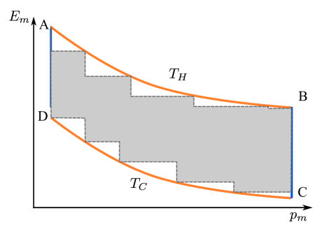
Figure 3: (Color online) Schematic illustration of a discrete Carnot cycle. This discrete Carnot-like thermodynamic cycle is composed by two discrete isothermal processes ($\textrm{A}\rightarrow\textrm{B}$ and $\textrm{C}\rightarrow\textrm{D}$) and two adiabatic processes ($\textrm{B}\rightarrow\textrm{C}$ and $\textrm{D}\rightarrow\textrm{A}$) . Here the discrete black dashed curve represents the discrete isothermal process, while the smooth orange solid curve represents the corresponding quasi-static isothermal process in the limit that the operation time approaches infinity. The gray area encircled by the two discrete curve represents the output work per cycle. The temperature of the high and low temperature bath are $T_{H}$ and $T_{C}$, respectively, and the operation time that the working substance contacts with them are $t_{H}$ and $t_{C}$, respectively.

The heat transfer of the QCL heat engine is written as $\sum_{j=1}^{N}E^{(j)}\delta p^{(j)}$ QIP2 ; heat-and-work , we can connect the heat absorb (release) from the heat bath $\Delta Q_{H}$ ($\Delta Q_{C}$) to the area $\Lambda_{H}$ ($\Lambda_{C}$) encircled by the high (low) temperature-related discrete black dashed curve and the horizon axis. Thus, the power and efficiency of such a QCL heat engine can be expressed by two characteristic areas as follows

$$P=\frac{W}{t_{H}+t_{C}}=\frac{\Lambda_{H}-\Lambda_{C}}{t_{H}+t_{C}}=\frac{\Delta\Lambda}{t_{H}+t_{C}},$$ (11)

$$\eta=\frac{W}{\Delta Q_{H}}=\frac{\Lambda_{H}-\Lambda_{C}}{\Lambda_{H}}=1-\frac{\Lambda_{C}}{\Lambda_{H}}.$$ (12)

Here, $\Delta\Lambda=\Lambda_{H}-\Lambda_{C}$ corresponds to the output work per cycle as represented by the gray area in Fig. 3. We have assumed the energy level is tuned very rapid in the two adiabatic processes ($\textrm{B}\rightarrow\textrm{C}$ and $\textrm{D}\rightarrow\textrm{A}$), so that the corresponding operation time is ignored. It can be seen from Fig. 3 that the area $\Lambda_{H}$ is smaller than the area $\Lambda_{H}^{(r)}$ encircled by the high temperature-related smooth orange solid curve and the horizon axis, i.e., $\Lambda_{H}<\Lambda_{H}^{(r)}$. While the area $\Lambda_{C}$ is lager than the area $\Lambda_{C}^{(r)}$ encircled by the low temperature-related smooth orange solid curve and the horizon axis, i.e., $\Lambda_{C}>\Lambda_{C}^{(r)}$. Since $\Lambda_{H}^{(r)}$ and $\Lambda_{C}^{(r)}$ are connected to the reversible heat absorb and reversible heat release, respectively, the following inequality can be easily verified

$$\eta=1-\frac{\Lambda_{C}}{\Lambda_{H}}<1-\frac{\Lambda_{C}^{(r)}}{\Lambda_{H}^{(r)}}=\eta_{C}.$$ (13)

Following from Eq. (9), we obtain $\Lambda_{H}=T_{H}\Delta S_{H}-\xi_{H}\Theta_{H}/t_{H}$ and $\Lambda_{C}=T_{C}\Delta S_{C}-\xi_{C}\Theta_{C}/t_{C}$, where $\Delta S_{C}=\Delta S_{H}$ corresponds to the reversible part of the heat transfer in the whole cycle. Noticing the efficiency in Eq. (12) and the power in Eq. (11) are now connected with each other through the operation time $t_{C}$ and $t_{H}$. Thus, to find the EMP of the heat engine, one should optimize the power via the two operation times. With the framework developed by Esposito et. al. low-dissipation , the EMP of such heat engine reads

$$\eta_{\textrm{EMP}}=\frac{\eta_{C}\left(1+\sqrt{\frac{T_{C}\xi_{C}\Theta_{C}}{T_{H}\xi_{H}\Theta_{H}}}\right)}{\left(1+\sqrt{\frac{T_{C}\xi_{C}\Theta_{C}}{T_{H}\xi_{H}\Theta_{H}}}\right)^{2}+\frac{T_{C}}{T_{H}}\left(1-\frac{\xi_{C}\Theta_{C}}{\xi_{H}\Theta_{H}}\right)},$$ (14)

where we have replaced the phenomenological parameter $\Sigma$ in the original result of Ref. low-dissipation by our system and control scheme related parameters $\xi$ and $\Theta$, namely, $\Sigma_{\alpha}\rightarrow\xi_{\alpha}\Theta_{\alpha}$ ($\alpha=C,H$). Using the definition of $\Theta$ in Eq. (8) we have the ratio of $\Theta_{C}$ and $\Theta_{H}$ explicitly expressed as $\Theta_{C}/\Theta_{H}=\beta_{C}^{3}\Delta_{C}^{2}E_{C}^{(0)}\gamma_{C}^{-1}/\left(\beta_{H}^{3}\Delta_{H}^{2}E_{H}^{(0)}\gamma_{H}^{-1}\right)=\gamma_{H}/\gamma_{C}$. Here, we fix the four points A, B, C and D as the same as that in normal Carnot cycle with the relations $\beta_{H}E_{H}^{(0)}=\beta_{C}E_{C}^{(0)}$ and $\beta_{H}E_{H}^{(N)}=\beta_{C}E_{C}^{(N)}$. The operation time of each sub-process of the DIP is taken as $\tau_{\alpha}=2\widetilde{\gamma}_{\alpha}^{-1}=\beta_{\alpha}E_{\alpha}^{(0)}/\gamma_{\alpha}$ ($\alpha=C,H$). For a practical designed heat engine, we typically have $\gamma_{H}/\gamma_{C}$ fixed once the interaction between the system and the heat bath is given. Therefore, the EMP of such a heat engine only depends on the scheme that the working substance’s energy spectra being tuned, i.e., $\xi_{C}/\xi_{H}$. When the control function is exponential function, we choose the system’s energy spectra to be linearly tuned at the low temperature bath, that is, $n_{C}=1$, and the control function satisfies $f_{H}(t)\propto t^{n_{H}},n_{H}\gg 1$ at the high temperature bath. Then, the EMP is simplified as

$$\eta_{\textrm{EMP}}=\frac{\eta_{C}\left(1+\sqrt{\frac{2T_{C}}{n_{H}T_{H}}}\right)}{2-\eta_{C}+2\sqrt{\frac{2T_{C}}{n_{H}T_{H}}}}\approx\eta_{+}\left(1-\eta_{+}\sqrt{\frac{2(1-\eta_{C})}{n_{H}}}\right),$$ (15)

where $\eta_{+}=\eta_{C}/(2-\eta_{C})$.

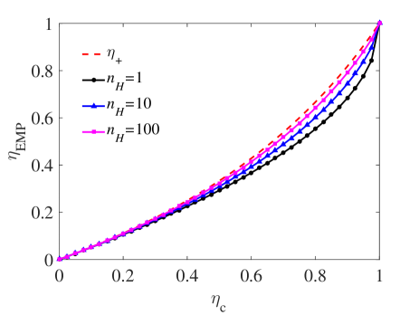
Figure 4: Efficiency at maximum power as function of Carnot efficiency, where the red dashed curve indicates the maximum value that the EMP can achieve $\eta_{+}=\eta_{C}/(2-\eta_{C})$. The black circle line represents the Curzon-Ahlborn efficiency with $n_{H}=n_{C}=1$, namely $f_{H}\propto t$. The blue triangle line and pink square line correspond to the control function in the high temperature discrete isothermal process being taken as $f_{H}\propto t^{10}$ and $f_{H}\propto t^{100}$, respectively.

In Fig. 4, we show the achievable EMP for different control functions. The dashed red line shows the maximum value $\eta_{+}$ of the EMP. And the black circle line represents the Curzon-Ahlborn efficiency $\eta_{\textrm{CA}}=1-\sqrt{1-\eta_{C}}$, which can be realized in our scheme with $n_{H}=n_{C}=1$. It can be seen from Eq. (15) that the EMP of the heat engine can be adjusted via different control functions, and can be significantly improved with $n_{H}$ increasing. The controllability of EMP is also demonstrated in Fig. 4 through the exact numerical results. With the increase of $n_{H}$, the EMP is deviating from $\eta_{\textrm{CA}}$ and getting closer to the upper bound of the EMP $\eta_{+}$. This means that it is feasible to control the EMP of the heat engines through different control schemes of tuning the system’s energy levels in the DIPs. Even with the constraint relation between power and efficiency TLA-heat-engine ; constriant2-1 ; constriant2 , we notice that one can maintain the maximum output power while increasing the EMP via different control schemes. Detailed discussion is shown in Appendix B.

The current control scheme with the stepwise Carnot-like cycle makes it possible for the experimental test by the widely-used setups experiment1 ; experiment2 ; experiment-trapped-ion for testing Jarzynski equality. Experiments concerning EMP were not feasible, to our best knowledge, because of unavailability of the control scheme. Our stepwise control scheme allows a clear separation of heat exchange and work extraction processes for implementing measurement. For the clarity, we consider the simple two-level atom case. In the DIP ($A\rightarrow B)$, we measure the probability sequences $p_{e}^{\left(0\right)}\rightarrow p_{e}^{\left(1\right)}\rightarrow p_{e}^{\left(2\right)}\rightarrow\cdots\rightarrow p_{e}^{\left(N-1\right)}\rightarrow p_{e}^{\left(N\right)}$ along with the energy level changes $E^{\left(0\right)}\rightarrow E^{\left(0\right)}\rightarrow E^{\left(2\right)}\rightarrow\cdots\rightarrow E^{\left(N-1\right)}\rightarrow E^{\left(N\right)}$. The heat absorbed is calculated as follow,

$$\Delta Q_{H}=\sum_{i=0}^{N-1}(p_{e}^{\left(i+1\right)}-p_{e}^{\left(i\right)})E^{\left(i+1\right)}.$$ (16)

The first test is the $\mathscr{C}/t$ relation in Eq. (10) with variation of the operation time $t_{f}$ as well as different control schemes listed in Table 1. The irreversible entropy generation $S^{\left(\mathrm{ir}\right)}$ is obtained as

$$S^{\left(\mathrm{ir}\right)}=\Delta S-\frac{\Delta Q_{H}}{T_{H}},$$ (17)

where $\Delta S=p_{e}^{\left(N\right)}\ln p_{e}^{\left(N\right)}+[1-p_{e}^{\left(N\right)}]\ln[1-p_{e}^{\left(N\right)}]-p_{e}^{\left(0\right)}\ln p_{e}^{\left(0\right)}+[1-p_{e}^{\left(0\right)}]\ln[1-p_{e}^{\left(0\right)}]$. The similar approach is applied for the DIP ($C\rightarrow D$) for the heat $\Delta Q_{C}$ directed to the low temperature bath. The power of the engine is obtained as $P=(\Delta Q_{H}-\Delta Q_{C})/(t_{H}+t_{C})$. To meet the requirement of operation time for the heat engine achieving the EMP low-dissipation , $t_{H}$ and $t_{C}$ follow $t_{H}=2\xi_{H}\Theta_{H}\left[1+\sqrt{T_{C}\xi_{C}\Theta_{C}/\left(T_{H}\xi_{H}\Theta_{H}\right)}\right]/\left(\eta_{C}\Delta S\right)$ and $t_{C}=t_{H}\sqrt{T_{C}\xi_{C}\Theta_{C}/\left(T_{H}\xi_{H}\Theta_{H}\right)}$, respectively. Here, $\xi_{\alpha}$ is determined by the specific form of the control function $f_{\alpha}(t)$ ($\alpha=C,H$) as demonstrated in Table. 1. $\Theta_{H}$ ($\Theta_{C}$) is related to the starting and ending point of the high (low) temperature DIP as given by Eq. (8). The efficiency for one specific control scheme is obtained as $\eta=(\Delta Q_{H}-\Delta Q_{C})/\Delta Q_{H}$.

IV Conclusion

In summary, by introducing the discrete isothermal process, we presented a general proof of the inverse relation between the irreversible entropy generation and time in finite time isothermal process, namely $S^{(\mathrm{ir})}=\mathscr{C}/t$, which is widely used for the actual heat engines within the low-dissipation region. Besides the system constants, we showed that the coefficient $\mathscr{C}$ of irreversible entropy generation also depends the control scheme when the system’s energy levels are tuned in the discrete isothermal process. Remarkably, the minimal irreversible entropy generation is achieved when the energy levels of the system are linearly tuned. This discovery allows us to design optimal heat engine cycle. With a two-level atomic heat engine as an illustration, we demonstrate that the EMP of the heat engine can be optimized by applying different control schemes when the working substance contacting with different heat baths. The controllability of EMP can be experimentally verified with some state of art experimental platforms, such as superconducting circuit system Pekola2009 , and trapped ion experiment1 ; experiment-trapped-ion .

Appendix A Evolution of the two level system

The dynamics of the two-level atom, when it contacts with a heat bath with inverse temperature $\beta=(k_{B}T)^{-1}$, is described by the master equation

$$\frac{dp_{e}\left(t\right)}{dt}=-\gamma\left(2n_{\mathrm{th}}[E(t)]+1\right)p_{e}\left(t\right)+\gamma n_{\mathrm{th}}[E(t)],$$ (18)

where $p_{e}\left(t\right)\equiv\langle e|\hat{\rho}\left(t\right)|e\rangle$ is the excited state population of the density matrix $\hat{\rho}\left(t\right)$, $\gamma$ the system-bath coupling strength, and $n_{\mathrm{th}}[E(t)]=1/\left(\exp[\beta E\left(t\right)]-1\right)$ the mean occupation number of bath mode with frequency $E\left(t\right)$. The solution of Eq. (18) reads

$$p_{e}(t)=\frac{n_{\mathrm{th}}[E(t)]}{1+2n_{\mathrm{th}}[E(t)]}(1-e^{-\gamma\left\{2n_{\mathrm{th}}[E(t)]+1\right\}t})+e^{-\gamma\left\{2n_{\mathrm{th}}[E(t)]+1\right\}t}p_{e}\left(0\right)\;,$$ (19)

applying which to the $j-$th step of the discrete isothermal process, we obatin

$$p_{e}\left(\tau\right)=p_{e}^{(j)}(1-e^{-\frac{1+e^{-\beta E^{(j)}}}{e^{-\beta E^{(j)}}-1}\gamma\tau})+e^{-\frac{1+e^{-\beta E^{(j)}}}{e^{-\beta E^{(j)}}-1}\gamma\tau}p_{e}^{(j-1)}.$$ (20)

In the high temperature limit, i.e. , $\beta E\ll 1$, the above equation can be simplified as

$$p_{e}\left(\tau\right)=p_{e}^{(j)}+e^{-\frac{2\gamma\tau}{\beta E^{(j)}}}\left(p_{e}^{(j-1)}-p_{e}^{(j)}\right).$$ (21)

Choosing $\tau=\beta E^{(0)}/\gamma$, one finds $\exp\left[-2\gamma\tau/\left(\beta E^{(j)}\right)\right]\approx e^{-2}\ll 1$, then $p_{e}\left(\tau\right)\rightarrow p_{e}^{(j)}$. The order of the error is about $e^{-2}$.

Appendix B Dependence of power on control scheme

For low-dissipation heat engines, the maximum power in Ref. TLA-heat-engine ; low-dissipation can be re-written with our notation as,

$$P_{max} =\frac{(\eta_{C}T_{h}\Delta S)^{2}}{4(\sqrt{T_{h}\xi_{h}\Theta_{h}}+\sqrt{T_{c}\xi_{c}\Theta_{c}})^{2}}$$ (22)

$$=\frac{(\eta_{C}T_{h}\Delta S)^{2}}{4T_{c}\xi_{c}\Theta_{c}}\left(1+\sqrt{\frac{T_{h}\xi_{h}\Theta_{h}}{T_{c}\xi_{c}\Theta_{c}}}\right)^{-2}.$$ (23)

It is clear that the maximum power depends on $\xi_{h}/\xi_{c}$ and $\xi_{c}$, while the EMP only depends on $\xi_{h}/\xi_{c}$ as shown in [Eq. (14)] of our manuscript. Therefore we can maintain the maximum power unchanged by fixing the value of

$$\xi_{c}^{-1}\left(1+\sqrt{\frac{T_{h}\xi_{h}\Theta_{h}}{T_{c}\xi_{c}\Theta_{c}}}\right)^{-2},$$ (24)

while improving the efficiency by increasing the ratio $\xi_{h}/\xi_{c}$.