Faster search for long gravitational-wave transients: GPU implementation of the transient $\mathcal{F}$-statistic

Abstract

The $\mathcal{F}$-statistic is an established method to search for continuous gravitational waves from spinning neutron stars. Prix et al. [1, (2011)] introduced a variant for transient quasi-monochromatic signals. Possible astrophysical scenarios for such transients include glitching pulsars, newborn neutron stars and accreting systems. Here we present a new implementation of the transient $\mathcal{F}$-statistic, using pyCUDA to leverage the power of modern graphics processing units (GPUs). The obtained speedup allows efficient searches over much wider parameter spaces, especially when using more realistic transient signal models including time-varying (e.g. exponentially decaying) amplitudes. Hence, it can enable comprehensive coverage of glitches in known nearby pulsars, improve the follow-up of outliers from continuous-wave searches, and might be an important ingredient for future blind all-sky searches for unknown neutron stars.

• LIGO-P1800031-v6 [draft version: 15 June 2018]

1 Introduction

Spinning neutron stars (NSs), when non-axisymmetrically deformed, emit weak but potentially detectable gravitational waves (GWs) [2]. Many searches [3] with the LIGO and Virgo detectors [4, 5] focus on continuous wave (CW) signals that are persistent over a whole observation run, but there are also scenarios for shorter signals from transiently perturbed NSs. If those signals are slowly evolving in frequency and last on the time scale of hours to months, analysis methods adapted from CW searches are well suited to their detection. In [1] (hereafter also referred to as ‘PGM’), the astrophysical motivation for such transient signals was discussed and a matched-filter search method proposed. It is based on the established $\mathcal{F}$-statistic, which was introduced in [6, 7] and used in many CW searches [recently e.g. in 8, 9, 10].

Matched-filter searches for weak signals from unknown sources (or those with imperfectly known parameters) are computationally very expensive since a wide parameter space needs to be densely covered with templates. Starting from a typical CW search that covers a certain parameter space in signal frequency, spindown and sky location but assumes a constant signal amplitude, the addition of new unknown parameters to describe the transient evolution further increases computational cost.

However, the attractiveness of the transient $\mathcal{F}$-statistic algorithm from [1] is that it starts from time-discretised quantities already computed for the standard CW $\mathcal{F}$-statistic and then only needs to take partial sums of these to study the set of possible transient signals. Still, for long total observation times the evaluation of these partial sums can easily dominate over the original computational cost, especially if the templates have a non-trivial amplitude evolution, e.g. exponential decay.

The task of multiple partial sums of some input data can obviously benefit from massive parallelisation. Here we present a straightforward translation of the algorithm from [1] to pyCUDA code [11] running on graphics processing units (GPUs). It is implemented in the framework of the PyFstat package [12, 13].

In the following, we briefly review the formalism from [1] to define the transient $\mathcal{F}$-statistic (section 2), then describe its pyCUDA implementation (section 3). We test the speed and memory requirements (section 4) and compare with the original CPU implementation from LALSuite [14]. The paper ends with a brief discussion (section 5) of how the achieved speedup widens the scope of feasible searches for long CW-like gravitational wave transients. This includes enabling a comprehensive coverage of glitch events in nearby known pulsars, improving the sensitivity of all-sky CW searches through following up more outliers with transient analyses, and the potential use as an ingredient in future blind all-sky searches for unknown disturbed NSs.

2 Formalism

We present a straightforward pyCUDA implementation of PGM’s ‘atoms-based’ transient $\mathcal{F}$-statistic algorithm from Appendix A1 of [1]. It is based on a discretised method to compute the overall $\mathcal{F}$-statistic introduced in [15] and described in detail in [16].

The $\mathcal{F}$-statistic (for transient or continuous signals) is essentially a likelihood-ratio test for a time series $x(t)$, comparing a signal hypothesis

$$\mathcal{H}_{{\mathrm{{\mathrm{t}}{\mathrm{{S}}}}}}:x(t)=n(t)+h(t,\lambda,\mathcal{A},\mathcal{T})$$ (1)

against the alternative hypothesis of pure Gaussian noise,

$$\mathcal{H}_{\mathrm{{G}}}:x(t)=n(t)\,.$$ (2)

The waveform model $h(t,\lambda,\mathcal{A},\mathcal{T})=\varpi(t,\mathcal{T})\,h(t,\lambda,\mathcal{A})$ for a slowly-evolving signal separates into a transient window function $\varpi(t,\mathcal{T})$ and the standard CW waveform $h(t,\lambda,\mathcal{A})$. The latter depends on a set of phase evolution parameters $\lambda=\{\alpha,\delta,f,{\dot{f}},\ddot{f},\dots\}$ (sky position, frequency, and frequency derivatives or ‘spindowns’) and on four amplitude parameters $\mathcal{A}=\{h_{0},\cos\iota,\psi,\phi_{0}\}$. See [1, 6, 16] for details on these parameters. For the transient part, we currently consider either rectangular or exponential window functions, with parameters $\mathcal{T}=\{t_{0},\tau\}$ where $t_{0}$ is the start time of a signal and $\tau$ is a duration parameter:

$$\varpi_{\mathrm{rect}}(t,t_{0},\tau):=\left\{\begin{array}[]{ll}1&\mbox{if }t\in[t_{0},t_{0}+\tau]\\ 0&\mbox{otherwise}\,,\end{array}\right.$$ (3)

$$\varpi_{\mathrm{exp}}(t,t_{0},\tau):=\left\{\begin{array}[]{ll}\mathrm{e}^{-(t-t_{0})/\tau}&\mbox{if }t\in[t_{0},t_{0}+3\tau]\\ 0&\mbox{otherwise}\,.\end{array}\right.$$ (4)

The cutoff of $\varpi_{\mathrm{exp}}$ at $3\tau$ was introduced in [1] in the understanding that the signal-to-noise ratio (SNR) after this point will be negligible.

The (transient) $\mathcal{F}$-statistic is then proportional to the log odds between $\mathcal{H}_{{\mathrm{{\mathrm{t}}{\mathrm{{S}}}}}}$ and $\mathcal{H}_{\mathrm{{G}}}$, after maximising over $\mathcal{A}$ (or marginalising, see [1, 17, 18] for details):

$$\mathrm{e}^{\mathcal{F}(x,\lambda,\mathcal{T})}\propto\frac{P\left(\mathcal{H}_{{\mathrm{{\mathrm{t}}{\mathrm{{S}}}}}}\middle|x,\lambda,\mathcal{T},\mathcal{I}\right)}{P\left(\mathcal{H}_{\mathrm{{G}}}\middle|x,\mathcal{I}\right)}\,.$$ (5)

It can be written as

$$\mathcal{F}(x,\lambda,\mathcal{T})=\frac{1}{2}x^{\prime}_{\mu}(\lambda,\mathcal{T})\,\mathcal{M}^{\prime\mu\nu}(\lambda,\mathcal{T})\,x^{\prime}_{\nu}(\lambda,\mathcal{T})\,,$$ (6)

where the indices $\mu$, $\nu$ run over the four amplitude parameters $\mathcal{A}$, $\mathcal{M}^{\prime\mu\nu}$ is the antenna pattern matrix, $x^{\prime}_{\mu}$ are projections of the data onto the model waveforms, and the prime denotes transient windowing. (See Eqs. (32–36) of [1].)

The standard algorithm used in $\mathcal{F}$-statistic searches for continuous signals splits a data set starting at $T_{0}$ and of length $T_{\mathrm{obs}}$ into several Short Fourier Transforms (SFTs) of length $T_{\mathrm{SFT}}$. [16] describes how to approximate (6) from the per-SFT, per-detector discretised versions of $\mathcal{M}^{\prime\mu\nu}$ and $x^{\prime}_{\mu}$; in practice we consider the equivalent set of quantities $\{a_{j},b_{j},F_{aj},F_{bj}\}$ as the atoms of our $\mathcal{F}$-statistic computation, where the $j$ index runs over SFTs.

The $a_{j}$ and $b_{j}$ atoms are summed up to yield the discretised antenna pattern matrix elements $\widehat{A}$, $\widehat{B}$, $\widehat{C}$ [defined in Eq. (130) of 16] and their determinant $\widehat{D}=\widehat{A}\,\widehat{B}-\widehat{C}^{2}$, and together with the summed data-dependent complex quantities $F_{a}$, $F_{b}$ [Eq.(129) of 16] they yield the $\mathcal{F}$-statistic as:

$$\mathcal{F}(x,\lambda,\mathcal{T})=\widehat{D}^{-1}\,( \widehat{B}\,[\,\Re^{2}(F_{a})+\Im^{2}(F_{a})\,]+\widehat{A}\,[\,\Re^{2}(F_{b})+\Im^{2}(F_{b})\,]$$

$$-2\widehat{C}\,[\,\Re(F_{a})\Re(F_{b})+\Im(F_{a})\Im(F_{b})\,]\,)\,.$$

(All quantities on the right hand side are understood as depending on $\lambda$ and $\mathcal{T}$, too.)

For persistent CWs, this is evaluated summing all atoms over the full $T_{\mathrm{obs}}$. To search for transient signals, we define a grid in $\{t_{0},\tau\}$ space indexed by $m$ for the $t_{0}$ dimension and $n$ for the $\tau$ dimension. We indicate the resolutions of this grid as $d{t_{0}}$ and $d{\tau}$; a natural choice is $d{t_{0}}=d{\tau}=T_{\mathrm{SFT}}$ though a coarser or even variable sampling is also possible. Then our goal is to compute, for each $\lambda$ and a specific window choice $\varpi$, the matrix

$$\mathcal{F}_{mn}(\lambda):=\mathcal{F}(x,\lambda,\varpi,t_{0\,m},\tau_{n})\,,$$ (8)

which we also refer to as the transient $\mathcal{F}$-statistic map. Computing it this way is convenient because the set of atoms $\{a_{j},b_{j},F_{aj},F_{bj}\}$ is only computed once, over the full $T_{\mathrm{obs}}$, and this is already done for the CW $\mathcal{F}$-statistic anyway. Subsequently, the transient $\mathcal{F}_{mn}$ map is obtained by evaluating (2) for partial sums of the atoms.

3 Implementation

PyFstat is a python package primarily developed for the MCMC follow-up [12, 13] of CW candidates, but it also provides general modular access to CW search functionality in the LALPulsar package (written in C) of the LALSuite [14] collection, called through SWIG C-to-python wrappers. For the transient $\mathcal{F}$-statistic, we first call a standard algorithm for computing the CW $\mathcal{F}$-statistic over the whole data set [16], which takes care of the data read-in, barycentring, and computation of the per-SFT matched-filter atoms. The only change is that we ask the ComputeFstat() routine to also return the atoms.

The input data for computing the transient $\mathcal{F}$-statistic map $\mathcal{F}_{mn}$ consists then of only the atoms (a set of vectors of $N_{\mathrm{SFT}}$ elements each) and the parameters describing a transient window function and grid in $\{t_{0},\tau\}$ space. The inputs are the 3 real vectors $a^{2}(t)$, $b^{2}(t)$ and $a(t)\cdot b(t)$ and the 2 complex vectors $F_{a}(t)$, $F_{b}(t)$. These are transferred to the GPU as a $7\times N_{\mathrm{SFT}}$ real matrix.

The basic idea of massively-parallelised computation on a GPU is to run a grid of identical kernels, each processing the subset of data identified by the kernel’s (multi-)index. We provide two structurally different kernels for rectangular and exponential windows. To account for the general case where resolutions in $t_{0}$ or $\tau$ different from $T_{\mathrm{SFT}}$ might be desirable, or where there are gaps in the data, we use $N_{t_{0}}$ and $N_{\tau}$ for the number of grid points in each dimension, which need not be equal to each other nor to $N_{\mathrm{SFT}}$.

In the rectangular case, an obvious optimisation was already pointed out in [1] and is implemented in LALPulsar: For each starting time $t_{0\,m}$, one can compute $\mathcal{F}_{mn}$ for all durations $\tau_{n}$ by keeping the partial sums of each atom up to each $\tau_{n^{\prime}}$ in memory and only adding the atoms with index $n^{\prime}+1$ in the next step. It would thus be wasteful to run a full $N_{t_{0}}\times N_{\tau}$ grid of kernels on the GPU, and instead we only launch $N_{t_{0}}$ kernels, each of which internally loops over $\tau$ and keeps the partial sums in local memory.

In the exponential case, no such simple trick is possible, since the contribution to each partial sum at each timestep includes amplitude-weight factors (see Eq. (4)) depending on the $\tau$ currently being evaluated. Hence, we employ a brute-force grid of $N_{t_{0}}\times N_{\tau}$ kernels on the GPU, each of which only computes the partial sums for a single $\mathcal{F}_{mn}$.

In both cases, the last steps, still done inside the GPU kernel, are to compute the antenna pattern matrix determinant $\widehat{D}$ and the transient $\mathcal{F}_{mn}$-statistic from Eq. (2).

4 Tests

In this section, we describe tests of the speedup obtained with the pyCUDA version, its memory requirements, and its numerical faithfulness to the original implementation.

4.1 Speed

We have tested the speed of the pyCUDA implementation relative to the standard LALPulsar code on several systems. These all have Intel CPUs: a laptop with a Core i5-6200U at 2.30 GHz, a workstation with a Xeon X5675 at 3.07 GHz and two LIGO Caltech cluster nodes with Xeons E5-2630 and E5-2650 at 2.20 GHz each. The pyCUDA code was benchmarked on several GPUs from the Nvidia GeForce GTX family (1050, 1060, 1070 and 1080Ti, with 2–11 GB RAM) and on a Nvidia Tesla V100-PCIE (16 GB RAM), all installed on the same workstation and cluster nodes.

We consider observation times $T_{\mathrm{obs}}$ from 1 hour up to 1 year, with no gaps in the data. Gaussian noise and a transient signal with $\tau=0.5\,T_{\mathrm{obs}}$ are simulated through PyFstat, though the speed of calculating $\mathcal{F}$-statistics does not depend on whether the data contains a signal. The SFTs are taken at $T_{\mathrm{SFT}}=1800$ s and $\mathcal{F}_{mn}$ is sampled at $d{t_{0}}=d{\tau}=T_{\mathrm{SFT}}$ over a grid of $t_{0}\in[T_{0},T_{\mathrm{obs}}-2T_{\mathrm{SFT}}]$ and $\tau\in[2T_{\mathrm{SFT}},T_{\mathrm{obs}}]$. The upper limit on $t_{0}$ and lower limit on $\tau$ are set because the low-level implementation requires at least 2 SFTs per $\mathcal{F}_{mn}$ computation.

Since GPU results for a single-template (fixed $\lambda$) analysis might be too pessimistic because of startup overheads, and in practice speedups are only relevant for searches over broad $\lambda$ regions anyway, we time searches over 100 frequency bins; though for simplicity we assume a fixed sky location and no spindown. Timing results are summarised in figure 1, as average runtime per $\lambda$ template. As an additional cross-check, these results also include some runs at 1000 frequency bins, which yield consistent timings per template. Note that this is the total runtime of the search (per template), including the initial LALPulsar computation of the atoms which always runs on the CPU.

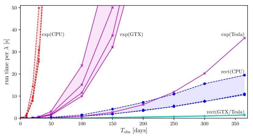
Figure 1: Timing results for both rectangular and exponential transient windows, from CPU (LALPulsar) and GPU (pyCUDA) implementations on various devices. The vertical axis gives the average run time per template $\lambda$. (Most test runs used 100 frequency bins, and a few used 1000 to check the consistency of averages.) Each solid/dashed line connects results from a specific implementation on a specific device, averaging over 3 or more runs at fixed $T_{\mathrm{obs}}$, and background shading indicates a specific window run on a family of related architectures. The exp(CPU) and rect(CPU) families collect results from the four different systems mentioned in Sec. 4.1, while exp(GTX) labels results from different Nvidia Geforce GXT 10x0 family devices, the single line labelled exp(Tesla) is from a Nvidia Tesla V100, and the rect(GTX/Tesla) results are plotted together as they are not significantly different.

We find that the pyCUDA version provides speedups of at least an order of magnitude on GPUs of the Geforce GTX 10x0 family compared to the original LALPulsar code on contemporaneous CPUs, both for exponential and rectangular windows. In the exponential case, the Tesla V100 provides another similar jump in speed over the GTX family, bringing the cost of exponential-window transient searches over hundreds of days down to a similar cost as with the standard rectangular LALPulsar CPU implementation.

We can also more directly compare these measurements to the timing model from Appendix A3 of [1]. We find that to cover arbitrary combinations of $\{T_{\mathrm{data}},N_{t_{0}},N_{\tau}\}$, we need to somewhat generalise the model. This is done in detail in our A. However, for the timings presented in figure 1, we are in regimes where the cost for rectangular windows is dominated by the $N_{t_{0}}\,N_{\tau}$ scaling and the cost for exponential windows is dominated by the $N_{\mathrm{sums}}$ scaling. The results, converted to the ‘timing constants’ as introduced in [1], are listed in table 1, and are generally consistent with fits of the more general timing model.

Table 1: Timing results from figure 1, fit assuming dominant $N_{t_{0}}\,N_{\tau}$ scaling for rectangular windows and $N_{\mathrm{sums}}$ scaling for exponential windows, and converted to the timing constants $\mathfrak{c}_{\mathrm{r}}$, $\mathfrak{c}_{\mathrm{e}}$ as introduced by [1]. Fit errors are $<1$%. See A for details and for complementary example fits of the more general timing model.
Note that $\mathfrak{c}_{\mathrm{e}}<\mathfrak{c}_{\mathrm{r}}$ for the GPUs does not mean that the overall search for an exponential window is faster than for a rectangular window, as these constants are multiplied with different summation counters, see (10) and (11).

• CPU/GPU	$\mathfrak{c}_{\mathrm{r}}$ [s]	$\mathfrak{c}_{\mathrm{e}}$ [s]
  Core2Duo 2.6 GHz	$4.2\cdot 10^{-8}$	$1.3\cdot 10^{-7}$	from [1]
  i5-6200U	$6.4\cdot 10^{-8}$	$1.1\cdot 10^{-7}$
  Xeon X5675	$3.5\cdot 10^{-8}$	$7.0\cdot 10^{-8}$
  Xeon E5-2630	$3.4\cdot 10^{-8}$	$5.7\cdot 10^{-8}$
  Xeon E5-2650	$3.6\cdot 10^{-8}$	$6.0\cdot 10^{-8}$
  GTX-1050	$6.1\cdot 10^{-9}$	$1.4\cdot 10^{-9}$
  GTX-1060	$4.8\cdot 10^{-9}$	$9.1\cdot 10^{-10}$
  GTX-1070	$4.2\cdot 10^{-9}$	$7.3\cdot 10^{-10}$
  GTX-1080	$4.4\cdot 10^{-9}$	$6.2\cdot 10^{-10}$
  Tesla-V100	$4.3\cdot 10^{-9}$	$4.6\cdot 10^{-11}$

4.2 Memory

GPU applications are often memory-limited. However, for the transient $\mathcal{F}$-statistic map, we do not expect GPU memory to be a significant constraint, as we see in the following. With the current approach, the input atoms need to be transferred to GPU memory only for a single $\lambda$ parameter space point at a time, then the $\mathcal{F}_{mn}(\lambda)$ matrix is computed and returned. Hence, the peak GPU memory usage of input plus output matrices is expected to be

$$M[\mathrm{bytes}]=4\,(\,7N_{\mathrm{SFT}}+N_{t_{0}}N_{\tau}\,)\,,$$ (9)

where 4 bytes is the base size of a real32 number in the underlying NumPy [19] package. While the input array size grows only linearly with $N_{\mathrm{SFT}}$, assuming $d{t_{0}}=d{\tau}=T_{\mathrm{SFT}}$ the $\mathcal{F}_{mn}$ matrix grows quadratically and will dominate memory usage at long $T_{\mathrm{obs}}$. However, in practice one might want to choose an undersampling of $t_{0}$, $\tau$.

A comparison of this expectation with practical memory usage measurements is presented in figure 2. For $T_{\mathrm{SFT}}=1800$ s and $d{t_{0}}=d{\tau}=T_{\mathrm{SFT}}$, the memory usage reaches only about 1.1 GB for a year of data, and with undersampling even much longer data sets would remain easily feasible on current GPUs, even when multiple jobs need to run on a single device.

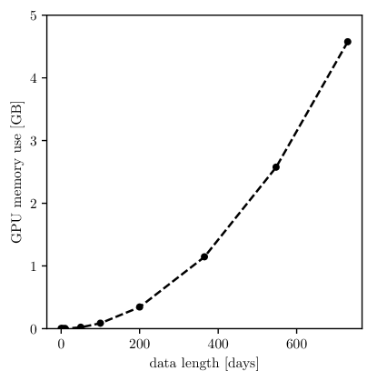
Figure 2: GPU memory usage on a GeForce GTX 1070 (8 GB RAM) with CUDA V8.0.61. Measured with $T_{\mathrm{SFT}}=1800$ s and a resolution of $d{t_{0}}=d{\tau}=T_{\mathrm{SFT}}$ at all $T_{\mathrm{obs}}$. Each data point is the difference between the output of a call to pycuda.driver.mem_get_info() right before allocating input and output arrays with pycuda.gpuarray, and a call right afterwards. The dashed line is the expected $4(7N_{\mathrm{SFT}}+N_{t_{0}}N_{\tau})$ scaling (in bytes). As $T_{\mathrm{obs}}\to 0$, we find that the base memory use for the kernel itself (and any other possible overheads) seems to be only about 2–4 MB.

4.3 Accuracy

The original LALPulsar implementation is already using single precision for the atoms and the $\mathcal{F}$-statistic itself, so in contrast to some other GPU use cases [20] it was not necessary to reduce the code’s internal precision for the pyCUDA version. However, the $\mathcal{F}$-statistic algorithm is already known to produce slightly different numerical results on different CPU platforms, so it is worth checking the typical amount of differences in the transient $\mathcal{F}$-statistic between LALPulsar and pyCUDA versions.

As demonstrated for a particular test case in figure 3, we typically find negligibly small differences, not larger than other implementation- and platform-dependent variations in the $\mathcal{F}$-statistic known from other work (e.g. [21]).

One implementation detail to note is that in the exponential case the LALPulsar implementation uses a lookup-table (LUT) based ‘fast exponential’ function. This can actually lead to differences with pyCUDA of up to $\sim 10$%, but figure 3 shows results after replacing it with the exp() function of the C standard library, thus verifying that the difference did not come from a loss of accuracy with the new pyCUDA implementation.

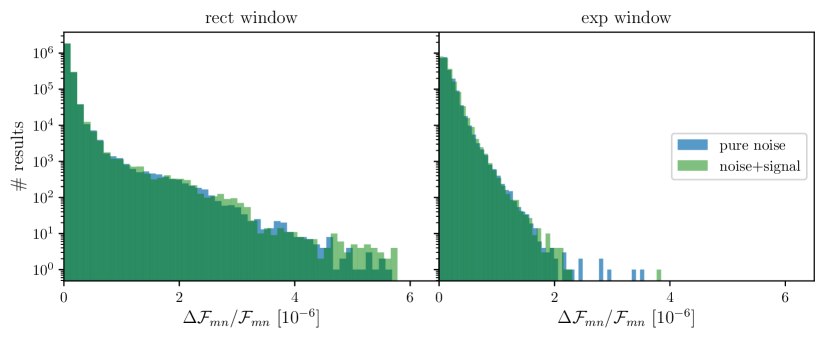
Figure 3: Comparison of $\mathcal{F}_{mn}$ computed with the LALPulsar and pyCUDA implementations. Each histogram gives the differences $\Delta\mathcal{F}_{mn}$ between the two implementations for a certain transient window, and either for pure Gaussian noise or also including a (confidently detectable, $\max 2\mathcal{F}\approx 263$) signal injection with matching window function. The histograms are taken over all individual $\mathcal{F}_{mn}$ values for 1000 frequency bins over a 1-day data set with $T_{\mathrm{SFT}}=1800$. The GPU for this test was a GeForce GTX 1070.

5 Conclusion and applications

The significant speedup achieved with our pyCUDA implementation of the transient $\mathcal{F}$-statistic will allow for a wider scope of searches for long-duration transient GWs. We now discuss a few example applications that would be hard resource-wise, or even prohibitive, on CPUs but could become viable with GPUs.

Let us first consider the natural use case of a GW data analysis triggered by radio observations of a pulsar glitch. Quasi-monochromatic GW emission, which the $\mathcal{F}$-statistic is sensitive to, could be associated with the post-glitch relaxation. Depending on the pulsar, this can have timescales of days to months [22, 23]. As a simple transient search setup, assume we look at a single fixed $t_{0}$ and at $\tau\in[2T_{\mathrm{SFT}},\,T_{\mathrm{obs}}=4\,\mathrm{months}]$ with $\delta\tau=T_{\mathrm{SFT}}=1800$s. With these parameters, we find a Tesla-V100 GPU outperforms a Xeon-E5 CPU by a runtime factor of $\approx 10$ for rectangular windows and $\approx 2300$ for exponential windows. Still, with a single GW search template matching the post-glitch radio timing solution (at $f_{\mathrm{GW}}=2f_{\mathrm{spin}}$), such an analysis would be computationally trivial even on a single CPU ($\approx 1700\mathrm{s}$ for exponential windows).

However, it would be reasonable to allow for some mismatch between the radio timing and GW frequency evolution due to the perturbed state of the NS after a glitch. For comparison, the ‘narrow-band’ search for CWs from known pulsars in the first aLIGO run [24] (using 121 days of data) covered some ranges in frequency $f$ and spindown ${\dot{f}}$ for each of its 11 targets, with totals of e.g. $2.2\cdot 10^{6}$ templates for the Vela pulsar and $1.6\cdot 10^{8}$ for the crab pulsar. (Using the corrected Table I as per the erratum [25] to [24].)

Multiplying these numbers of templates with the per-template transient $\mathcal{F}$-statistic cost (which in this setup again dominates over the rest of the $\mathcal{F}$-statistic search code), we find that a single Tesla-V100 GPU could perform an exponential-window transient analysis over the Vela band in less than 3 weeks, while the same analysis would take 120 years on a single Xeon-E5-like CPU; or equivalently would require over 2300 CPUs to only take the same 3 weeks as the single GPU.

Meanwhile, for the wider Crab analysis range (which is due to its strong spindown), even the GPU would still need 4 years (compared to 9000 years for a single CPU). While we can trivially further parallelise the problem by splitting the $(f,{\dot{f}})$ space over multiple GPUs, only a small number of such devices are available on current computing clusters. We can gain some more speed-up by reducing the sampling in $\tau$, but in the end the parameter space for the Crab would need to be somewhat reduced in practice.

In summary, performing routine transient $\mathcal{F}$-statistic analyses of all observed glitches in known galactic pulsars during a GW observation run – with reasonably wide $f$ and ${\dot{f}}$ bands (similar to those used in [24], or only slightly reduced) – becomes feasible with a few dedicated GPU systems.

Similar estimates apply when considering the follow-up [26, 27, 12] of significant or marginal detection candidates produced by wide-parameter space CW searches [3]. Even though those searches target perfectly persistent signals, they can also produce candidates if there are sufficiently strong transient events in the data [28]. A comprehensive transient-aware follow-up, with the goal of either verifying the presumed persistent nature or uncovering a transient signal instead, needs to not only target the exact phase-evolution parameters $\lambda$ of the candidate, but search a wider band around it to account for degeneracies with the transient evolution parameters. Reducing the computational cost of each candidate’s follow-up directly translates into a larger number of candidates that can be analysed, so that the overall threshold of the CW search can be lowered and a better search sensitivity can be achieved.

The data length and $\{t_{0},\tau\}$ ranges in this scenario can be longer than in the EM-triggered post-glitch scenario: the aLIGO runs O1–O3 took data for / are scheduled for 4, 9 and 12 months respectively [29], and for the follow-up of a strong candidate data from multiple observing runs could get combined. The range of phase evolution parameters $\lambda$ that should be searched for full coverage depends on the exact setup of the CW search and on possible intermediate follow-up steps; but the scaling of the transient $\mathcal{F}$-statistic cost is similar as in the EM-triggered case (see A for the full timing model) and the improvements in accessible search volume using a small number of GPUs over CPUs will be similar.

In the longer term, untriggered all-sky searches for long-duration transients are of high interest. Similarly to all-sky CW searches, they have the potential to discover a population of electromagnetically dark NSs, for example glitching pulsars with their beam pointed away from Earth. The sensitivity of all-sky searches is directly limited by how densely they can cover the $\lambda$ parameter space at a fixed computational budget. [30, 31]. Hence, adding transient parameters at first significantly reduces the overall sensitivity of a blind search. But speeding up the transient part by orders of magnitude could still make a combined search for CWs and transients feasible in the long run, when large numbers of GPUs become available in high-performance clusters or through Einstein@Home [32]. In practice, though, the more promising approach for blind transient searches might be to apply a cheap add-on transient modification, like that introduced in [28], to a semi-coherent CW algorithm as a first search stage, then apply the fully-coherent transient $\mathcal{F}$-statistic only in a follow-up step.

In any of these scenarios, while we have focussed on the fact that the pyCUDA version can bring down the cost of exponential-windowed transients significantly, the cost for rectangular windows always remains smaller, so that in practice whenever exponential windows are feasible, it is also cheap and natural to run both analyses and evaluate a posteriori which one fits the data better. Different window functions for the amplitude evolution could also be considered, and would generically follow the GPU kernel grid setup and timing model for the exponential window, since it does not assume any function-specific optimisations.

Appendix

Appendix A Generalising the PGM2011 timing model

Here we revisit the timing model for computing $\mathcal{F}_{mn}$ maps introduced in Appendix A3 of [1]. Their equations (A13) and (A14) give the computing cost for a single-$\lambda$ $\mathcal{F}_{mn}$ map with either exponential

$$\mathfrak{c}^{\mathrm{e}}_{\mathcal{F}\mathrm{map}}\approx\mathfrak{c}_{\mathrm{e}}\,\frac{\Delta t_{0}}{d{t_{0}}}\,\frac{\Delta\tau}{d{\tau}}\,\frac{(\tau_{\min}+\Delta\tau/2)}{T_{\mathrm{SFT}}}\approx\mathfrak{c}_{\mathrm{e}}\,N_{t_{0}}\,N_{\tau}\,\frac{(\tau_{\min}+\Delta\tau/2)}{T_{\mathrm{SFT}}}$$ (10)

or rectangular window functions:

$$\mathfrak{c}^{\mathrm{r}}_{\mathcal{F}\mathrm{map}}=\mathfrak{c}_{\mathrm{r}}\,\frac{\Delta t_{0}}{d{t_{0}}}\,\frac{(\tau_{\min}+\Delta\tau)}{T_{\mathrm{SFT}}}\approx\mathfrak{c}_{\mathrm{r}}\,N_{t_{0}}\,\frac{(\tau_{\min}+\Delta\tau)}{T_{\mathrm{SFT}}}=\mathfrak{c}_{\mathrm{r}}\,N_{t_{0}}\,\frac{\tau_{\max}}{T_{\mathrm{SFT}}}\,.$$ (11)

The timing constants $\mathfrak{c}_{\mathrm{e}}$ and $\mathfrak{c}_{\mathrm{r}}$ are interpreted as the cost to compute the (weighted) sums over atoms at each step. The exponential model corresponds to a ‘generic’ case where all quantities have to be re-evaluated at each step, while the rectangular case reuses partial sums as discussed before.

We note now that this formulation of the timing model does not explicitly include the cost of computing the antenna pattern matrix determinant $\widehat{D}$ and the $\mathcal{F}$-statistic itself, which is done once for each $(m,n)$ pair after all sums have been computed and hence is independent of the window function choice. We can include this contribution by adding a term $+\mathfrak{c}_{\mathcal{F}}\,N_{t_{0}}N_{\tau}$ to both cases. It will be very subdominant for exponential windows, where the summations term grows much faster than $N_{t_{0}}N_{\tau}$, but can be relevant for rectangular windows where the summations term is more efficient.

Another small contribution to the timing model is from setup and index-lookup costs that scale with the total number of SFTs handed to the $\mathcal{F}$-statistic-map function; for completeness we include a common term $\mathfrak{c}_{\mathrm{SFTs}}\,N_{\mathrm{SFT}}$.

In addition, Eqs. (10) and (11) only hold true if the full range of transient signal durations explored by the $\mathcal{F}_{mn}$ map is fully contained within the available data range, that is when $t_{0\max}+\tau_{\max}<T_{0}+T_{\mathrm{data}}$. (We call this the ‘embedded’ case below.) Otherwise, i.e. if some of the transient windows overlap the end of the available data, by convention the LALPulsar code still returns results for the full rectangular $\mathcal{F}_{mn}$ matrix, but truncates the atoms summations. Thus, the total computing cost in such cases is lower than estimated by Eqs. (10), (11) and using them to fit the timing constants from runtime measurements as in Sec. 4.1 would yield inconsistent results.

Hence, we generalise the PGM timing model by introducing $N_{\mathrm{sums}}$ as the effective number of summation steps for an $\mathcal{F}_{mn}$ map, which depends on the window type, $T_{\mathrm{data}}$, and the ranges of both $t_{0}$ and $\tau$:

$$\mathfrak{c}^{\mathrm{e}}_{\mathcal{F}\mathrm{map}}\approx\mathfrak{c}_{\mathrm{SFTs}}\,N_{\mathrm{SFT}}+\mathfrak{c}^{\mathrm{e}}_{\mathrm{sums}}\,N_{\mathrm{sums}}^{\mathrm{e}}+\mathfrak{c}_{\mathcal{F}}\,N_{t_{0}}\,N_{\tau}\,,$$ (12)

$$\mathfrak{c}^{\mathrm{r}}_{\mathcal{F}\mathrm{map}}\approx\mathfrak{c}_{\mathrm{SFTs}}\,N_{\mathrm{SFT}}+\mathfrak{c}^{\mathrm{r}}_{\mathrm{sums}}\,N_{\mathrm{sums}}^{\mathrm{r}}+\mathfrak{c}_{\mathcal{F}}\,N_{t_{0}}\,N_{\tau}\,.$$ (13)

For rectangular windows, we have

$$N_{\mathrm{sums}}^{\mathrm{r}}=\sum\limits_{m=1}^{N_{t_{0}}}\frac{\min(T_{\mathrm{data}}-t_{0\,m},\,\tau_{\max})}{T_{\mathrm{SFT}}}\,,$$ (14)

which reduces to PGM’s $N_{\mathrm{sums}}^{\mathrm{r}}=N_{t_{0}}\tau_{\max}/T_{\mathrm{SFT}}$ in the special ‘embedded’ case that PGM considered, and to $N_{\mathrm{sums}}^{\mathrm{r}}=0.5N_{t_{0}}\tau_{\max}/T_{\mathrm{SFT}}$ in the special case of $N_{t_{0}}d{t_{0}}=N_{\tau}d{\tau}=T_{\mathrm{data}}-2T_{\mathrm{SFT}}$ that we used for the timing results in Sec. 4.1.

For exponential windows, we also need to note that the current code’s convention, as introduced in Eq. (18) of [1], is that an exponential window with duration parameter $\tau$ covers an effective length of $3\tau/T_{\mathrm{SFT}}$ atoms. (The exponential decay is not cut off after only one, but after three e-folds, where the remaining SNR would be much more negligible.) Hence, PGM’s original timing constant $\mathfrak{c}_{\mathrm{e}}$ effectively contains a factor of 3 (from counting all steps in $\tau$) that we now include in $N_{\mathrm{sums}}^{\mathrm{e}}$ instead:

$$N_{\mathrm{sums}}^{\mathrm{e}}=\sum\limits_{m=1}^{N_{t_{0}}}\sum\limits_{n=1}^{N_{\tau}}\frac{\min(T_{\mathrm{data}}-t_{0\,m},\,3\,\tau_{n})}{T_{\mathrm{SFT}}}\,.$$ (15)

In the ‘embedded’ case this reduces to $3N_{t_{0}}\sum\limits_{n=1}^{N_{\tau}}\tau_{n}/T_{\mathrm{SFT}}=3N_{t_{0}}N_{\tau}(\tau_{\min}+0.5\Delta\tau)/T_{\mathrm{SFT}}$, equivalent to PGM’s result up to the factor of 3.

In practice, on each architecture we can use these more general equations (12)–(15) to fit the four timing constants $\{\mathfrak{c}_{\mathrm{SFTs}},\mathfrak{c}_{\mathcal{F}},\mathfrak{c}^{\mathrm{r}}_{\mathrm{sums}},\mathfrak{c}^{\mathrm{e}}_{\mathrm{sums}}\}$ from a variety of setups (in terms of $T_{\mathrm{data}}$, $[t_{0\min},t_{0\max}]$, $[\tau_{\min},\tau_{\max}]$), then consider the special ‘embedded’ case (and $N_{\tau}\gg 1$, $\tau_{\max}\gg\tau_{\min}$) to directly compare to [1] by

$$\mathfrak{c}_{\mathrm{r}}=\mathfrak{c}^{\mathrm{r}}_{\mathrm{sums}}+\frac{T_{\mathrm{SFT}}}{\tau_{\max}}\left(\mathfrak{c}_{\mathrm{SFTs}}\frac{N_{\mathrm{SFT}}}{N_{t_{0}}}+\mathfrak{c}_{\mathcal{F}}\,N_{\tau}\right)\approx\mathfrak{c}^{\mathrm{r}}_{\mathrm{sums}}+\mathfrak{c}_{\mathcal{F}}\,,$$ (16)

$$\mathfrak{c}_{\mathrm{e}}=3\mathfrak{c}^{\mathrm{e}}_{\mathrm{sums}}+\frac{T_{\mathrm{SFT}}}{\tau_{\min}+0.5\Delta\tau}\left(\mathfrak{c}_{\mathrm{SFTs}}\frac{N_{\mathrm{SFT}}}{N_{t_{0}}N_{\tau}}+\mathfrak{c}_{\mathcal{F}}\right)\approx 3\mathfrak{c}^{\mathrm{e}}_{\mathrm{sums}}+\frac{2}{N_{\tau}}\mathfrak{c}_{\mathcal{F}}\approx 3\mathfrak{c}^{\mathrm{e}}_{\mathrm{sums}}\,.$$ (17)

Using a set of timing runs that in addition to those in section 4.1 also cover many different combinations of $\{T_{\mathrm{data}},N_{t_{0}},N_{\tau}\}$, and also measuring only the executation time of the actual $\mathcal{F}$-statistic map function (while in section 4.1 the whole search call is timed, including the contribution of computing the atoms, which is usually subdominant but not in the limit of low $N_{t_{0}}\,N_{\tau}$ and $N_{\mathrm{sums}}$), we do a detailed fit of the full timing model of (12) and (13), in the following iterative steps to ensure convergence:

1. fit the $\mathfrak{c}_{\mathrm{SFTs}}\,N_{\mathrm{SFT}}$ term only to short data sets with $N_{\mathrm{sums}}\leq 100$

2. using this fixed $\mathfrak{c}_{\mathrm{SFTs}}$, fit $\mathfrak{c}^{\mathrm{r}}_{\mathrm{sums}}\,N_{\mathrm{sums}}^{\mathrm{r}}+\mathfrak{c}_{\mathcal{F}}\,N_{t_{0}}\,N_{\tau}$ for rectangular windows

3. using fixed $\mathfrak{c}_{\mathrm{SFTs}}$ and $\mathfrak{c}_{\mathcal{F}}$, fit $\mathfrak{c}^{\mathrm{e}}_{\mathrm{sums}}\,N_{\mathrm{sums}}^{\mathrm{e}}$ for exponential windows

We find e.g.

$$\mathfrak{c}^{\mathrm{r}}_{\mathcal{F}\mathrm{map}}\approx\left((2.80\pm 0.03)N_{\mathrm{SFT}}+(0.96\pm 0.08)N_{\mathrm{sums}}^{\mathrm{r}}+(5.59\pm 0.06)N_{t_{0}}N_{\tau}\right)10^{-8}\,\mathrm{s}$$ (18)

$$\mathfrak{c}^{\mathrm{e}}_{\mathcal{F}\mathrm{map}}\approx\left((2.80\pm 0.03)N_{\mathrm{SFT}}+(3.55\pm 0.03)N_{\mathrm{sums}}^{\mathrm{e}}+(5.59\pm 0.06)N_{t_{0}}N_{\tau}\right)10^{-8}\,\mathrm{s}$$ (19)

for the i5-6200U laptop CPU (corresponding to PGM constants $\mathfrak{c}_{\mathrm{r}}=(6.36\pm 0.08)10^{-8}$ and $\mathfrak{c}_{\mathrm{e}}=(1.07\pm 0.01)10^{-7}$); and

$$\mathfrak{c}^{\mathrm{r}}_{\mathcal{F}\mathrm{map}}\approx\left((2.59\pm 0.02)N_{\mathrm{SFT}}+(0.27\pm 0.02)N_{\mathrm{sums}}^{\mathrm{r}}+(3.09\pm 0.02)N_{t_{0}}N_{\tau}\right)10^{-8}\,\mathrm{s}$$ (20)

$$\mathfrak{c}^{\mathrm{e}}_{\mathcal{F}\mathrm{map}}\approx\left((2.59\pm 0.02)N_{\mathrm{SFT}}+(2.22\pm 0.03)N_{\mathrm{sums}}^{\mathrm{e}}+(3.09\pm 0.02)N_{t_{0}}N_{\tau}\right)10^{-8}\,\mathrm{s}$$ (21)

for the Xeon X5675 workstation CPU (corresponding to PGM constants $\mathfrak{c}_{\mathrm{r}}=(3.26\pm 0.02)10^{-8}$ and $\mathfrak{c}_{\mathrm{e}}=(6.67\pm 0.08)10^{-8}$). These results agree reasonably well with those obtained on the same systems, but with fixed $N_{t_{0}},N_{\tau}$ in relation to $T_{\mathrm{data}}$ and with simplified fits, as presented in table 1. While the error bars from fitting alone appear too small to explain the remaining differences of 0.5–7%, it is likely that variations in system configuration and load between timing runs are the main culprit.

References

- [1] Prix R, Giampanis S and Messenger C 2011 Phys. Rev. D 84 023007 [arXiv:1104.1704]
- [2] Prix R (for the LIGO Scientific Collaboration) 2009 Gravitational Waves from Spinning Neutron Stars (Astrophys. Space Sci. Lib. vol 357) (Springer Berlin Heidelberg) chap 24, pp 651–685 ISBN 978-3-540-76964-4 URL https://dcc.ligo.org/LIGO-P060039/public
- [3] Riles K 2017 Mod. Phys. Lett. A32 1730035 [arXiv:1712.05897]
- [4] Aasi J et al. (LIGO Scientific Collaboration) 2015 Class. Quant. Grav. 32 074001 [arXiv:1411.4547]
- [5] Acernese F et al. (Virgo Collaboration) 2015 Class. Quant. Grav. 32 024001 [arXiv:1408.3978]
- [6] Jaranowski P, Królak A and Schutz B F 1998 Phys. Rev. D 58 063001 [arXiv:gr-qc/9804014]
- [7] Cutler C and Schutz B F 2005 Phys. Rev. D 72 063006 [arXiv:gr-qc/0504011]
- [8] Aasi J et al. (LIGO Scientific Collaboration and Virgo Collaboration) 2015 Astrophys. J. 813 39 [arXiv:1412.5942]
- [9] Zhu S J et al. 2016 Phys. Rev. D 94 082008 [arXiv:1608.07589]
- [10] Abbott B P et al. (LIGO Scientific Collaboration and Virgo Collaboration) 2017 Phys. Rev. D 96 122004 [arXiv:1707.02669]
- [11] Klöckner A, Pinto N, Lee Y, Catanzaro B, Ivanov P and Fasih A 2012 Parallel Computing 38 157–174 ISSN 0167-8191
- [12] Ashton G and Prix R 2018 [arXiv:1802.05450]
- [13] Ashton G and Keitel D 2018 Pyfstat-v1.2 URL https://doi.org/10.5281/zenodo.1243931
- [14] LSC Algorithm Library - LALSuite (free software) URL https://git.ligo.org/lscsoft/lalsuite
- [15] Williams P R and Schutz B F 1999 AIP Conf. Proc. 523 473 [arXiv:gr-qc/9912029]
- [16] Prix R 2015 The F-statistic and its implementation in ComputeFStatistic_v2 Tech. Rep. LIGO-T0900149 URL https://dcc.ligo.org/LIGO-T0900149/public
- [17] Prix R and Krishnan B 2009 Class. Quant. Grav. 26 204013 [arXiv:0907.2569]
- [18] Keitel D, Prix R, Papa M A, Leaci P and Siddiqi M 2014 Phys. Rev. D 89 064023 [arXiv:1311.5738]
- [19] Oliphant T E 2006 A guide to NumPy (Trelgol Publishing)
- [20] Navarro C A, Hitschfeld-Kahler N and Mateu L 2014 Communications in Computational Physics 15 285–329
- [21] Prix R 2011 F-statistic bias due to noise-estimator Tech. Rep. LIGO-T1100551 URL https://dcc.ligo.org/LIGO-T1100551/public
- [22] Lyne A G, Shemar S L and Smith F G 2000 Mon. Not. R. Astron. Soc. 315 534–542
- [23] Haskell B and Antonopoulou D 2014 Mon. Not. Roy. Astron. Soc. 438 16 [arXiv:1306.5214]
- [24] Abbott B P et al. (Virgo, LIGO Scientific) 2017 Phys. Rev. D96 122006 [arXiv:1710.02327]
- [25] Abbott B P et al. (Virgo, LIGO Scientific) 2018 Phys. Rev. D97 129903
- [26] Shaltev M and Prix R 2013 Phys. Rev. D 87 084057 [arXiv:1303.2471]
- [27] Papa M A et al. 2016 Phys. Rev. D 94 122006 [arXiv:1608.08928]
- [28] Keitel D 2016 Phys. Rev. D 93 084024 [arXiv:1509.02398]
- [29] Abbott B P et al. (VIRGO, LIGO Scientific) 2018 Living Rev. Rel. 21:3 [arXiv:1304.0670] URL https://link.springer.com/article/10.1007/s41114-018-0012-9
- [30] Prix R and Shaltev M 2012 Phys. Rev. D 85 084010 [arXiv:1201.4321]
- [31] Wette K 2012 Phys. Rev. D 85 042003 [arXiv:1111.5650]
- [32] Allen B et al. Einstein@Home distributed computing project URL https://einsteinathome.org