A nonconforming Trefftz virtual element method for the Helmholtz problem

Abstract

We introduce a novel virtual element method (VEM) for the two dimensional Helmholtz problem endowed with impedance boundary conditions. Local approximation spaces consist of Trefftz functions, i.e., functions belonging to the kernel of the Helmholtz operator. The global trial and test spaces are not fully discontinuous, but rather interelement continuity is imposed in a nonconforming fashion. Although their functions are only implicitly defined, as typical of the VEM framework, they contain discontinuous subspaces made of functions known in closed form and with good approximation properties (plane waves, in our case). We carry out an abstract error analysis of the method, and derive $h$-version error estimates. Moreover, we initiate its numerical investigation by presenting a first test, which demonstrates the theoretical convergence rates.

AMS subject classification: 35J05, 65N12, 65N15, 65N30

Keywords: virtual element method, Trefftz methods, nonconforming methods, Helmholtz problem, plane waves, polygonal meshes

1 Introduction

The virtual element method (VEM) is a recent generalization of the finite element method (FEM) to polytopal grids [6, 7]. It has been investigated in connection with a widespread number of problems and engineering applications, a short list of them being [46, 10, 39, 8, 11, 14]. In particular, VEM where the continuity constraints are imposed in a nonconforming way have been the object of an extensive study [3, 16, 15, 24, 2, 47, 30, 33].

The main feature of VEM is that test and trial spaces consist of functions that are not known in closed form, but that are solutions to local differential problems mimicking the target one. Despite this fact, the method is made fully computable by defining two tools, namely suitable mappings from local approximation spaces into spaces of known functions (typically polynomials), and suitable bilinear/sesquilinear stabilization forms.

For the Helmholtz problem, a virtual version of the classical partition of unity method [4] was introduced in [41]. That method is based on discrete approximation functions given by the product of low order harmonic VE functions with plane waves.

In this work, we present a novel VE approach for the Helmholtz equation, which differs from the plane wave VEM of [41] in the two following aspects: in our method

• local test and trial spaces consist of functions that belong to the kernel of the Helmholtz operator;

• no global $H^{1}$-conformity in the approximation space is required; instead, zero jumps of Dirichlet traces across interfaces are imposed in a nonconforming fashion.

This new method, which will be referred to as nonconforming Trefftz-VEM, does not fall into the partition of unity setting, but rather into the Trefftz one. On the other hand, it also differs from the Trefftz methods in the Helmholtz literature, which typically employ fully discontinuous trial and test functions; this is the case of the ultra weak variational formulation [17], plane wave discontinuous Galerkin methods [27], discontinuous methods based on Lagrange multipliers [22], wave based methods [19], the least square formulation [38], and of the variational theory of complex rays [42]; see [28] for a survey.

The nonconforming approach adopted here provides an elegant theoretical framework, where the best approximation error for Trefftz-VE functions can be bounded in terms of the best approximation error for piecewise discontinuous Trefftz functions. Such property is not valid, at the best of our understanding, when employing conforming spaces. This extends a results of [33], where the best approximation error for nonconforming harmonic VE functions was bounded by that for piecewise discontinuous harmonic polynomials. In this sense, the nonconforming approach in the Trefftz-VE technology provides a common framework for problems of different nature.

The nonconforming Trefftz-VEM thus extends the nonconforming harmonic VEM of [33], which in turn was a nonconforming version of the harmonic VEM of [18], to the Helmholtz problem. It has the advantages of Trefftz methods, as it reduces considerably the number of degrees of freedom needed for achieving a given accuracy as compared to standard polynomial methods. At the same time, it makes use of basis functions with some sort of continuity. To be more precise, the impedance traces of the functions in the nonconforming Trefftz-VE spaces at the boundaries of the mesh elements are prescribed to be traces of plane waves, and the degrees of freedom are chosen to be Dirichlet moments on each edge with respect to plane waves; this allows to build global spaces with continuity of such Dirichlet moments. In this way, information regarding the behavior of the discrete solution on the mesh skeleton can be recovered. As compared to the partition of unity approach [4], the nonconforming Trefftz-VEM  neither needs to have at disposal an explicit partition of unity nor requires volume quadrature formulas. This however comes at the price of substituting the original sesquilinear form with a computable one.

In the construction of the method, we start with a larger number of degrees of freedom than for other Trefftz methods, e.g. plane wave discontinuous Galerkin method. However, as the basis functions are associated with the mesh edges, an edgewise orthogonalization-and-filtering process, as described in [34], allows to significantly reduce the number of degrees of freedom without deteriorating the accuracy. The numerical experiments presented in [34] show that the nonconforming approach becomes in this way competitive with other Trefftz methods.

The structure of the paper is the following. After presenting the model problem and some notation, we introduce in Section 2 the functional setting and we describe in Section 3 the nonconforming Trefftz-VE method. An abstract error analysis and $h$-version error estimates are derived in Section 4. Finally, we present a numerical test in Section 5 and we state some conclusions in Section 6.

We refer to [34] a wide set of numerical experiments of the $h$-, the $p$-, and the $hp$-versions of the method, the comparison with other methods, and the description of its implementation aspects, including the orthogonalization-and-filtering process.

Model problem.

The model problem we consider is the following. Given a bounded convex polygon $\Omega\subset\mathbb{R}^{2}$ with boundary $\partial\Omega$, and $g\in H^{-\frac{1}{2}}(\partial\Omega)$, we consider the homogeneous Helmholtz problem with impedance boundary condition

$$\left\{\begin{aligned} -\Delta u-k^{2}u&=0&&\quad\text{ in }\Omega,\\ \nabla u\cdot\textbf{{n}}_{\Omega}+\textup{i}ku&=g&&\quad\text{ on }\partial\Omega,\end{aligned}\right.$$ (1)

where $k>0$ is the wave number, i is the imaginary unit, and $\mathbf{n}_{\Omega}$ denotes the unit normal vector on $\partial\Omega$ pointing outside $\Omega$.

The corresponding variational formulation reads

$$\begin{cases}\text{find }u\in V\text{ such that}\\ b(u,v)=\int_{\partial\Omega}g\overline{v}\,\text{d}s\quad\forall v\in V,\\ \end{cases}$$ (2)

where $V:=H^{1}(\Omega)$ and where

$$b(u,v):=a(u,v)+\textup{i}k\int_{\partial\Omega}u\overline{v}\,\text{d}s\quad\forall u,\,v\in V,$$ (3)

with

$$a(u,v):=\int_{\Omega}\nabla u\cdot\overline{\nabla v}\,\text{d}x-k^{2}\int_{\Omega}u\overline{v}\,\text{d}x\quad\forall u,\,v\in V.$$

Problem (2) is well-posed for all wave numbers $k$ and, due to the convexity assumption on $\Omega$, $u\in H^{2}(\Omega)$, if we assume in addition $g\in H^{\frac{1}{2}}(\partial\Omega)$, see e.g. [36, Proposition 8.1.4].

Notation.

We will employ the standard notation for Sobolev spaces, norms, seminorms, and sesquilinear forms with values in the complex field $\mathbb{C}$. More precisely, given $s\in\mathbb{N}$ and $D\subset\mathbb{R}^{d}$, $d\in\leavevmode\nobreak\ \mathbb{N}$, $H^{s}(D,\mathbb{C})=:H^{s}(D)$ denotes the space of Lebesgue measurable functions with $s$ square integrable weak derivatives. Sobolev spaces with fractional order can be defined, e.g. via interpolation theory [45]. The standard norms, seminorms, and inner products are denoted, respectively, by

$$\|\cdot\|_{s,D},\quad\quad|\cdot|_{s,D},\quad\quad(\cdot,\cdot)_{s,D}.$$

We highlight separately the definition of the $H^{\frac{1}{2}}(\partial D)$ inner product:

$$(u,v)_{\frac{1}{2},\partial D}=(u,v)_{0,\partial D}+\int_{\partial D}\int_{\partial D}\frac{(u(\boldsymbol{\xi})-u(\boldsymbol{\eta}))\overline{(v(\boldsymbol{\xi})-v(\boldsymbol{\eta}))}}{|\boldsymbol{\xi}-\boldsymbol{\eta}|^{2}}d\boldsymbol{\xi}\,d\boldsymbol{\eta},$$

where $|\cdot|$ denotes the Euclidean distance.

Moreover, given $r\in\mathbb{R}$, we denote by $\mathbb{R}_{>r}$ and $\mathbb{R}_{\geq r}$ the set of all real numbers that are greater than, and greater than or equal to $r$, respectively; in addition, given $m\in\mathbb{N}$, we denote by $\mathbb{N}_{\geq m}$ the set of all natural numbers that are greater than or equal to $m$. We define by $B_{r}(\mathbf{x}_{0})$ the ball centered at $\mathbf{x}_{0}\in\mathbb{R}^{2}$ and with radius $r$.

Finally, we highlight that, given two positive quantities $a$ and $b$, we write $a\lesssim b$ in lieu of $a\leq c\,b$ for some positive constant $c$ independent of the discretization parameters and on the problem data.

2 The functional setting

In this section, we discuss some tools which are instrumental for the construction of the method. More precisely, we firstly introduce the concept of regular polygonal decompositions of the physical domain in Section 2.1. In Section 2.2, we recall some functional inequalities and we define broken Sobolev spaces and plane wave spaces.

2.1 Regular polygonal decompositions and assumptions

We introduce here the concept of regular polygonal decompositions of the physical domain $\Omega$.

Given $\{\mathcal{T}_{n}\}_{n\in\mathbb{N}}$ a sequence of polygonal decompositions of $\Omega$, for every $n\in\mathbb{N}$ we denote by $\mathcal{E}_{n}$, $\mathcal{E}_{n}^{I}$ and $\mathcal{E}_{n}^{B}$ the set of edges, interior edges, and boundary edges, respectively. Moreover, for any polygon $K\in\mathcal{T}_{n}$, we denote by $\mathcal{E}^{K}$ the set of its edges and we define

$$h_{K}:=\textup{diam}(K),\quad n_{K}:=\textup{card}(\mathcal{E}^{K}).$$

We also define the local sesquilinear form

$$a^{K}(u,v):=\int_{K}\nabla u\cdot\overline{\nabla v}\,\text{d}x-k^{2}\int_{K}u\overline{v}\,\text{d}x\quad\forall u,v\in H^{1}(K).$$ (4)

Note that

$$a(u,v)=\sum_{K\in\mathcal{T}_{n}}a^{K}(u,v)\quad\forall u,\,v\in V.$$

Finally, given any $e\in\mathcal{E}^{K}$, we denote by $h_{e}$ its length.

For a given mesh, we define its mesh size by

$$h:=\underset{K\in\mathcal{T}_{n}}{\max}\,h_{K},$$

A sequence of polygonal decompositions $\{\mathcal{T}_{n}\}_{n\in\mathbb{N}}$ is said to be regular if the following geometric assumptions are satisfied:

• (uniform star-shapedness) there exist $\rho\in(0,\frac{1}{2}]$, $0<\rho_{0}\leq\rho$, such that, for all $n\in\mathbb{N}$ and for all $K\in\mathcal{T}_{n}$, there exist points $\mathbf{x}_{0,K}\in K$ for which the ball $B_{\rho h_{K}}(\mathbf{x}_{0,K})$ is contained in $K$, and $K$ is star-shaped with respect to $B_{\rho_{0}h_{K}}(\mathbf{x}_{0,K})$;

• (uniformly non-degenerating edges) for all $n\in\mathbb{N}$ and for all $K\in\mathcal{T}_{n}$, it holds $h_{e}\geq\rho_{0}h_{K}$ for all edges $e$ of $K$, where $\rho_{0}$ is the same constant as in (G1);

• (uniform boundedness of the number of edges) there exists a constant $\Lambda\in\mathbb{N}$ such that, for all $n\in\mathbb{N}$ and for all $K\in\mathcal{T}_{n}$, $n_{K}\leq\Lambda$, i.e., the number of edges of each element is uniformly bounded.

2.2 Broken Sobolev spaces and plane wave spaces

Given $K\in\mathcal{T}_{n}$, we denote the impedance trace of a function $v\in H^{1}(K)$ on $\partial K$ by

$$\gamma_{I}^{K}(v):=\nabla v\cdot\textbf{{n}}_{K}+\textup{i}kv,$$ (5)

where $\textbf{{n}}_{K}$ is the unit normal vector on $\partial K$ pointing outside $K$. We recall the following trace inequality, see e.g. [23]:

$$\lVert v\rVert^{2}_{0,\partial K} \leq C_{T}\left(h_{K}^{-1}\lVert v\rVert^{2}_{0,K}+h_{K}\lvert v\rvert^{2}_{1,K}\right)\quad\forall v\in H^{1}(K),$$ (6)

where $C_{T}$ depends solely on the shape of $K$. Further, we recall the following Poincaré-Friedrichs inequalities, see e.g. [13]:

$$\lVert\xi\rVert_{0,K}\leq C_{P}h_{K}\left(\lvert\xi\rvert_{1,K}+\text{meas}(\Upsilon)^{-1}\left|\int_{\Upsilon}\xi\,\text{d}s\right|\right)\quad\forall\xi\in H^{1}(K),$$ (7)

$$\lVert\xi\rVert_{0,K}\leq C_{P}h_{K}\left(\lvert\xi\rvert_{1,K}+h_{K}^{-2}\left|\int_{K}\xi\,\text{d}x\right|\right)\quad\forall\xi\in H^{1}(K),$$ (8)

where $\Upsilon$ is a measurable subset of $\partial K$ with 1D positive measure, and $C_{P}>0$ depends only on the shape of $K$.

Remark 1.

The constants appearing in the inequalities (6), (7), and (8), depend on the shape of the domain $K$. It can be proven that, if such inequalities are applied to the elements in the polygonal decompositions $\mathcal{T}_{n}$ above, then these constants depend solely on the parameters $\rho$ and $\Lambda$ introduced in the assumptions (G1)-(G2)-(G3), see [31] . For the sake of simplicity, we will avoid to mention such a dependence, whenever it is clear from the context.

Next, we define the broken Sobolev spaces of order $s$, for all $s\in\mathbb{N}$, subordinated to a decomposition $\mathcal{T}_{n}$,

$$H^{s}(\mathcal{T}_{n}):=\prod_{K\in\mathcal{T}_{n}}H^{s}(K)=\{v\in L^{2}(\Omega):v_{|_{K}}\in H^{s}(K)\quad\forall K\in\mathcal{T}_{n}\},$$

together with the corresponding broken Sobolev seminorms and the weighted broken Sobolev norms

$$\lvert v\rvert^{2}_{s,\mathcal{T}_{n}}:=\sum_{K\in\mathcal{T}_{n}}|v|^{2}_{s,K},\quad\lVert v\rVert_{s,k,\mathcal{T}_{n}}^{2}:=\sum_{K\in\mathcal{T}_{n}}\lVert v\rVert_{s,k,K}^{2},$$

respectively, where, for every $K\in\mathcal{T}_{n}$,

$$\lVert v\rVert_{s,k,K}^{2}:=\sum_{j=0}^{s}k^{2(s-j)}\lvert v\rvert_{j,K}^{2}.$$ (9)

Now, we define the plane wave spaces. To this purpose, given $p=2q+1$ for some $q\in\mathbb{N}$, we introduce the set of indices $\mathcal{J}:=\{1,\dots,p\}$ and the set of pairwise different normalized directions $\{\textbf{{d}}_{\ell}\}_{\ell\in\mathcal{J}}$. For every $K\in\mathcal{T}_{n}$ and $\ell\in\mathcal{J}$, we define the plane wave traveling along the direction $\textbf{{d}}_{\ell}$ as

$$w_{\ell}^{K}(\textbf{{x}}):=e^{\textup{i}k\textbf{{d}}_{\ell}\cdot(\textbf{{x}}-\textbf{{x}}_{K})}{}_{|_{K}},$$ (10)

and we define the local plane wave space on the element $K\in\mathcal{T}_{n}$ by

$$\mathbb{PW}_{p}(K):=\textup{span}\left\{w_{\ell}^{K}\,,\,\ell\in\mathcal{J}\right\}.$$ (11)

We make the following assumption on the plane wave directions:

• (minimum angle) there exists a constant $0<\delta\leq 1$ with the property that the directions $\{\textbf{{d}}_{\ell}\}_{\ell\in\mathcal{J}}$ are such that the minimum angle between two directions is larger than or equal to $\frac{2\pi}{p}\delta$, and the angle between two neighbouring directions is strictly smaller than $\pi$.

The global discontinuous plane wave space with uniform $p$ is given by

$$\mathbb{PW}_{p}(\mathcal{T}_{n}):=\prod_{K\in\mathcal{T}_{n}}\mathbb{PW}_{p}(K)=\{v\in L^{2}(\Omega):v_{|_{K}}\in\mathbb{PW}_{p}(K)\quad\forall K\in\mathcal{T}_{n}\}.$$

For the same $p$, we also introduce the spaces of traces of plane waves on the mesh edges. Given $e\in\mathcal{E}_{n}$, we define, for any $\ell\in\mathcal{J}$,

$$w_{\ell}^{e}(\textbf{{x}}):=e^{\textup{i}k\textbf{{d}}_{\ell}\cdot(\textbf{{x}}-\textbf{{x}}_{e})}\,_{|_{e}}.$$ (12)

We observe that, while the dimension of $\mathbb{PW}_{p}(K)$ is equal to $p$ for all $K\in\mathcal{T}_{n}$, the dimension of $\textup{span}\{w_{\ell}^{e},\,\ell\in\mathcal{J}\}$ could in principle be smaller. In fact, if

$$\textbf{{d}}_{j}\cdot(\textbf{{x}}-\textbf{{x}}_{e})=\textbf{{d}}_{\ell}\cdot(\textbf{{x}}-\textbf{{x}}_{e})\quad\forall\textbf{{x}}\in e$$ (13)

for some $j,\ell\in\{1,\dots,p\}$, $j>\ell$, then $w_{j}^{e}(\textbf{{x}})=w_{\ell}^{e}(\textbf{{x}})$.

Thus, we have to check for all the indices in $\mathcal{J}$ whether (13) is satisfied. Whenever this is the case, we remove, without loss of generality, the index $j$ from $\mathcal{J}$. This procedure is defined as the filtering process. We denote by $\mathcal{J}_{e}^{\prime}$ the resulting set of indices after the filtering process. Clearly, it holds $\textup{card}(\mathcal{J}_{e}^{\prime})\leq p$.

In addition to plane waves, in the forthcoming analysis (see Section 4) we will need to employ constant functions on the edges. To this purpose, we observe that, if there exists a direction $\textbf{{d}}_{*}\in\{\textbf{{d}}_{\ell}\}_{\ell\in\mathcal{J}}$ such that

$$\textbf{{d}}_{*}\cdot(\textbf{{x}}-\textbf{{x}}_{e})=0\quad\forall\textbf{{x}}\in e,$$ (14)

that is, $\textbf{{d}}_{*}$ is orthogonal to the edge $e$, then $\textup{span}\{w_{\ell}^{e},\,\ell\in\mathcal{J}_{e}^{\prime}\}$ already contains the constant functions. Therefore, we proceed as follows.

If there exists an index $t\in\mathcal{J}_{e}^{\prime}$ such that $\mathbf{d}_{t}$ fulfils (14), we simply set $\mathcal{J}_{e}:=\mathcal{J}_{e}^{\prime}$; otherwise, we define $\mathcal{J}_{e}:=\mathcal{J}_{e}^{\prime}\cup\{p+1\}$ and set $w_{p+1}^{e}(\textbf{{x}}):=1$. Finally, we set $p_{e}:=\textup{card}(\mathcal{J}_{e})$.

With these definitions of the set of indices $\mathcal{J}_{e}$ and of the corresponding functions $w_{\ell}^{e}$ on each edge $e\in\mathcal{E}_{n}$, we define the plane wave trace space of dimension $p_{e}$ as

$$\mathbb{PW}_{p}^{c}(e):=\textup{span}\left\{w_{\ell}^{e}\,,\,\ell\in\mathcal{J}_{e}\right\},$$ (15)

where the superscript $c$ indicates that the space includes the constants.

We denote the space of piecewise discontinuous traces over $\partial K$ as

$$\mathbb{PW}_{p}^{c}(\partial K)=\{w^{\partial K}\in L^{2}(\partial K):w^{\partial K}{}_{|_{e}}\in\mathbb{PW}_{p}^{c}(e)\quad\forall e\in\mathcal{E}^{K}\}.$$ (16)

In Figure 1, we depict the filtering process applied to all the possible configurations along a given edge $e\in\mathcal{E}^{K}$.

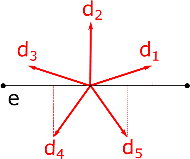
(a) No direction eliminated, orthogonal direction already included.

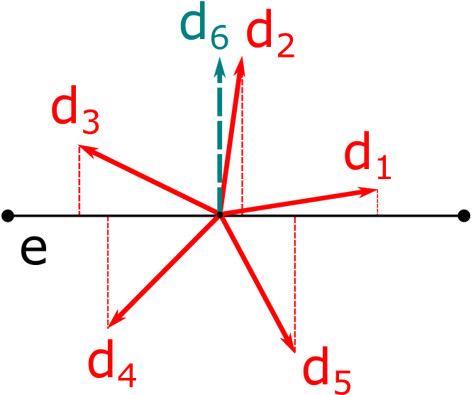
(b) No direction eliminated, orthogonal direction not yet included.

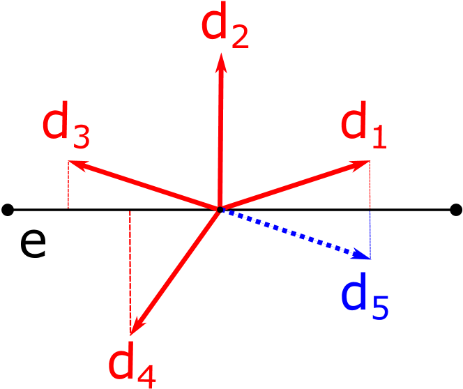
(c) One direction eliminated, orthogonal direction already included.

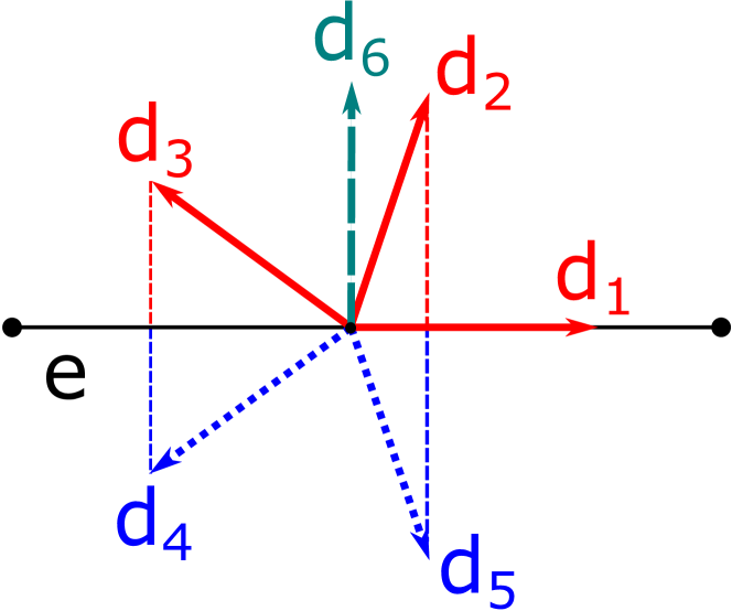
(d) Two directions eliminated, orthogonal direction not yet included.

Figure 1: Filtering process. We depict all the possible configurations. In solid lines, the directions that are kept; in dotted lines, the directions that are eliminated accordingly with (13); in dashed lines, the orthogonal direction that has to be possibly added in order to include constants.

We finally introduce the global nonconforming Sobolev space $H^{1,nc}(\mathcal{T}_{n})$. To this end, we need to fix some additional notation. In particular, given any internal edge $e\in\mathcal{E}_{n}^{I}$ shared by the polygons $K^{-}$ and $K^{+}$ in $\mathcal{T}_{n}$, we denote by $\mathbf{n}_{K^{\pm}}^{e}$ the two outer normal unit vectors with respect to $\partial K^{\pm}$. For the sake of simplicity, when no confusion occurs, we will write $\mathbf{n}_{K^{\pm}}$ in lieu of $\mathbf{n}_{K^{\pm}}^{e}$. Having this, for any $v\in H^{1}(\mathcal{T}_{n})$, we define the jump operator across an edge $e\in\mathcal{E}^{I}_{n}$ as

$$\llbracket v\rrbracket:=v_{|_{K^{+}}}\mathbf{n}_{K^{+}}+v_{|_{K^{-}}}\mathbf{n}_{K^{-}}.$$

Notice that $\llbracket v\rrbracket$ is vector-valued.

The global nonconforming Sobolev space with respect to the decomposition $\mathcal{T}_{n}$ and underlying plane wave spaces with parameter $p\in\mathbb{N}$, reads

$$H^{1,nc}(\mathcal{T}_{n}):=\left\{v\in H^{1}(\mathcal{T}_{n}):\,\int_{e}\llbracket v\rrbracket\cdot\mathbf{n}^{e}\,\overline{w^{e}}\,\text{d}s=0\,\quad\forall w^{e}\in\mathbb{PW}_{p}^{c}(e),\,\forall e\in\mathcal{E}_{n}^{I}\right\},$$ (17)

where $\mathbf{n}^{e}$ is either $\mathbf{n}_{K^{+}}^{e}$ or $\mathbf{n}_{K^{-}}^{e}$, but fixed.

3 Nonconforming Trefftz virtual element methods

In this section, we construct a nonconforming Trefftz-VEM for the approximation of solutions to the Helmholtz boundary value problem (2) and derive a priori error estimates.

Our aim is to design a numerical method having the following structure:

$$\begin{cases}\text{find }u_{h}\in V_{h}\text{ such that}\\ b_{h}(u_{h},v_{h})=F_{h}(v_{h})\quad\forall v_{h}\in V_{h},\\ \end{cases}$$ (18)

where, for all $n\in\mathbb{N}$, $V_{h}$ is a finite dimensional space subordinated to the mesh $\mathcal{T}_{n}$, $b_{h}(\cdot,\cdot)\leavevmode\nobreak\ :V_{h}\times V_{h}\to\mathbb{C}$ is a computable sesquilinear form mimicking its continuous counterpart $b(\cdot,\cdot)$ defined in (3), and the functional $F_{h}(\cdot):\,V_{h}\to\mathbb{C}$ is a computable counterpart of $\int_{\partial\Omega}g\overline{v}\,\text{d}s$.

The reason why we do not employ the continuous sesquilinear forms and right-hand side is that the functions in the nonconforming Trefftz-VE spaces are not known in closed form; therefore, the continuous sesquilinear forms and right-hand side are not computable.

The outline of this section is the following. In Section 3.1, local Trefftz-VE spaces, as well as the global space $V_{h}$ in (18), are introduced. Then, in Section 3.2, local projectors mapping from the local Trefftz-VE spaces into spaces of plane waves are defined; such projectors will allow to define suitable $b_{h}(\cdot,\cdot)$ and $F_{h}(\cdot)$ in (18), see Section 3.3. We point out that we do not discuss here the details of the implementation, but we refer the reader to [34].

3.1 Nonconforming Trefftz virtual element spaces

The aim of this section is to specify the nonconforming Trefftz-VE space $V_{h}$ that defines the method in (18).

Given $p\in\mathbb{N}$, for every $n\in\mathbb{N}$ and $K\in\mathcal{T}_{n}$, we first introduce the local Trefftz-VE space

$$V_{h}(K):=\left\{v_{h}\in H^{1}(K)\,\,|\,\,\Delta v_{h}+k^{2}v_{h}=0\,\text{ in }K,\quad\gamma_{I}^{K}(v_{h})_{|_{e}}\in\mathbb{PW}_{p}^{c}(e)\;\forall e\in\mathcal{E}^{K}\right\},$$ (19)

where we recall that $\gamma_{I}^{K}$ is defined in (5) and $\mathbb{PW}_{p}^{c}(e)$ is given in (15). In words, this space consists of all functions in $H^{1}(K)$ in the kernel of the Helmholtz operator, whose impedance traces are edgewise equal to traces of plane waves including constants.

It can be easily seen that $\mathbb{PW}_{p}(K)\subset V_{h}(K)$. However, the space $V_{h}(K)$ also contains other functions not available in closed form, whence the term virtual in the name of the method.

For each $K\in\mathcal{T}_{n}$, the dimension $p_{K}$ of the discrete space $V_{h}(K)$ in (19) coincides with the sum over all $e\in\mathcal{E}^{K}$ of the dimension $p_{e}$ of the edge plane wave spaces $\mathbb{PW}_{p}^{c}(e)$ in (15). Therefore, we have

$$p_{K}:=\dim V_{h}(K)=\sum_{e\in\mathcal{E}^{K}}p_{e},$$

where we recall that $p_{e}\leq p+1$.

Having this, we define the set of local degrees of freedom on $K\in\mathcal{T}_{n}$ as the moments on each edge $e\in\mathcal{E}^{K}$ with respect to functions in the space $\mathbb{PW}_{p}^{c}(e)$ defined in (15). More precisely, given $v_{h}\in V_{h}(K)$, its degrees of freedom are

$$\textup{dof}_{e,\ell}(v_{h})=\frac{1}{h_{e}}\int_{e}v_{h}\overline{w_{\ell}^{e}}\,\text{d}s\quad\forall e\in\mathcal{E}^{K},\,\forall\ell\in\mathcal{J}_{e}.$$ (20)

Besides, we denote by $\{\varphi_{e,\ell}\}_{e\in\mathcal{E}^{K},\,\ell\in\mathcal{J}_{e}}$ the local canonical basis, where

$$\textup{dof}_{\widetilde{e},\widetilde{\ell}}(\varphi_{e,\ell})=\delta_{(e,\ell),(\widetilde{e},\widetilde{\ell})}=\begin{cases}1&\text{if }(e,\ell)=(\widetilde{e},\widetilde{\ell})\\ 0&\text{otherwise}.\\ \end{cases}$$ (21)

We prove that the set of degrees of freedom (20) is unisolvent for all $K\in\mathcal{T}_{n}$, provided that the following assumption on the wave number $k$ is satisfied:

• the wave number $k$ is such that $k^{2}$ is not a Dirichlet-Laplace eigenvalue on $K$ for all $K\in\mathcal{T}_{n}$.

For a given $K\in\mathcal{T}_{n}$, the assumption (A1) results in a condition on the product $h_{K}k$. To be more precise, for any simply connected element $K$, the smallest Dirichlet-Laplace eigenvalue on $K$ satisfies

$$\lambda_{1}\geq\frac{a}{\rho_{K}^{2}},$$

where $\rho_{K}$ denotes the radius of the largest ball contained in $K$ and where $a\geq 0.6197$, see e.g. [5].

As a consequence, assuming that

$$h_{K}k\leq\sqrt{c_{0}a}$$ (22)

for some $c_{0}\in(0,1]$, we deduce

$$k^{2}=\frac{h_{K}^{2}k^{2}}{h_{K}^{2}}\leq\frac{c_{0}a}{h_{K}^{2}}\leq\frac{c_{0}a}{\rho_{K}^{2}}\leq\lambda_{1},$$

which means that the condition (22) guarantees that $k^{2}$ is not a Dirichlet-Laplace eigenvalue on $K$.

Lemma 3.1.

Suppose that the assumption (A1) holds true. Then, for every $K\in\mathcal{T}_{n}$, the set of degrees of freedom (20) is unisolvent for $V_{h}(K)$.

Proof.

Given $K\in\mathcal{T}_{n}$, we first observe that the dimension of the local space $V_{h}(K)$ is equal to the number of functionals in (20). Thus, we only need to prove that, given any $v_{h}\in V_{h}(K)$ such that all degrees of freedom (20) are zero, then $v_{h}=0$.

To this end, we observe that an integration by parts, together with the fact that $v_{h}$ belongs to the kernel of the Helmholtz operator, yields

$$\begin{split}&|v_{h}|^{2}_{1,K}-k^{2}\|v_{h}\|^{2}_{0,K}-\textup{i}k\|v_{h}\|^{2}_{0,\partial K}=\int_{K}\nabla v_{h}\cdot\overline{\nabla v_{h}}\,\text{d}x-k^{2}\int_{K}v_{h}\overline{v_{h}}\,\text{d}x-\textup{i}k\int_{\partial K}v_{h}\overline{v_{h}}\,\text{d}s\\ &=\int_{K}v_{h}\overline{\underbrace{(-\Delta v_{h}-k^{2}v_{h})}_{=0}}\,\text{d}x+\int_{\partial K}v_{h}\overline{(\nabla v_{h}\cdot\textbf{{n}}_{K}+\textup{i}kv_{h})}\,\text{d}s=\sum_{e\in\mathcal{E}^{K}}\int_{e}v_{h}\overline{\gamma_{I}^{K}(v_{h})_{|_{e}}}\,\text{d}s=0,\\ \end{split}$$ (23)

where in the last identity we also used the facts that, owing to the definition of the space $V_{h}(K)$ in (19), the impedance trace of $v_{h}$ is an element of the space (16), and that the degrees of freedom (20) of $v_{h}$ are zero. Thus, the imaginary part on the left-hand side of (23) is zero and one deduces that $v_{h}=0$ on $\partial K$. Since $v_{h}$ is also solution to a homogeneous Helmholtz equation, the assertion follows thanks to the assumption (A1). ∎

The global Trefftz-VE space is given by

$$V_{h}:=\{v_{h}\in H^{1,nc}(\mathcal{T}_{n}):\,v_{h|_{K}}\in V_{h}(K)\quad\forall K\in\mathcal{T}_{n}\},$$ (24)

where $H^{1,nc}(\mathcal{T}_{n})$ is defined in (17) with the same uniform $p$ as in the definition of the local Trefftz-VE spaces in (19). Consequently, the set of global degrees of freedom is obtained by coupling the local degrees of freedom on the interfaces between elements.

We underline that the definition of the degrees of freedom (20) is actually tailored for building discrete trial and test spaces that are nonconforming in the sense of (17). Besides, they will be used in the construction of projectors mapping onto spaces of plane waves. This is the topic of the next Section 3.2.

Remark 2.

Under the choice of the degrees of freedom in (20), the dimension of the global space is larger than that of plane wave discontinuous Galerkin methods [37]. However, at the practical level, an edge-by-edge orthogonalization-and-filtering process can be implemented, in order to reduce the dimension of the nonconforming Trefftz-VE space without losing in terms of accuracy. This procedure is described in detail in [34]. There, it is also observed that the two methods have a comparable behavior in terms of accuracy versus number of degrees of freedom and, in some occasions, the method presented herein performs better.

3.2 Local projectors

In this section, we introduce local projectors mapping functions in local Trefftz-VE spaces (19) onto plane waves. Such projectors will play a central role in the construction of the computable sesquilinear form $b_{h}(\cdot,\cdot)$ and functional $F_{h}(\cdot)$ for the method (18).

To start with, given $K\in\mathcal{T}_{n}$, we define the local projector

$$\begin{split}\Pi_{p}^{K}:\,&V_{h}(K)\rightarrow\mathbb{PW}_{p}(K)\\ &a^{K}(\Pi_{p}^{K}u_{h},w^{K})=a^{K}(u_{h},w^{K})\quad\forall u_{h}\in V_{h}(K),\,\forall w^{K}\in\mathbb{PW}_{p}(K).\end{split}$$ (25)

Note that this projector is computable by means of the degrees of freedom (20) without the need of explicit knowledge of the functions of $V_{h}(K)$. Indeed, an integration by parts and the fact that any plane wave $w^{K}\in\mathbb{PW}_{p}(K)$ belongs to the kernel of the Helmholtz operator lead to

$$\begin{split}a^{K}(u_{h},w^{K})&=\int_{K}\nabla u_{h}\cdot\overline{\nabla w^{K}}\,\text{d}x-k^{2}\int_{K}u_{h}\overline{w^{K}}\,\text{d}x\\ &=\sum_{e\in\mathcal{E}^{K}}\int_{e}u_{h}\overline{(\nabla w^{K}\cdot\textbf{{n}}_{K})}\,\text{d}s\quad\forall u_{h}\in V_{h}(K),\,\forall w^{K}\in\mathbb{PW}_{p}(K).\\ \end{split}$$

Since $(\nabla w^{K}\cdot\mathbf{n})_{K|_{e}}\in\mathbb{PW}_{p}^{c}(e)$ for all $e\in\mathcal{E}^{K}$, computability is guaranteed by the choice of the degrees of freedom in (20).

In the following proposition we prove that $\Pi_{p}^{K}$ is well-defined.

Proposition 3.2.

Assume that $K$ is an element of a mesh that satisfies the assumption (G1). Then, the following two statements hold true:

1. Denoting by $\mu_{2}$ the smallest positive Neumann-Laplace eigenvalue in $K$, it holds

   $$\mu_{2}\geqslant\frac{C_{\Delta}\pi^{2}}{h^{2}_{K}},$$

   where $C_{\Delta}\in(0,1]$ only depends on the shape of $K$, i.e., on $\rho_{0}$ and $\rho$ in the assumption (G1).

2. Assume that the assumption (D1) holds true. If $h_{K}k$ is such that there exists a constant $C_{1}>0$ with

   $$0<h_{K}k<C_{1}\leq\min\left\{\frac{\sqrt{C_{\Delta}}\pi}{\sqrt{2}},0.5538\right\},$$

   then $k^{2}<\mu_{2}$, and in particular it follows that $\Pi_{p}^{K}$ is well-defined and continuous. More precisely, there exists a constant $\beta(h_{K}k)>0$, uniformly bounded away from zero as $h_{K}k\to 0$, such that

   $$\lVert\Pi_{p}^{K}u_{h}\rVert_{1,k,K}\leq\frac{1}{\beta(h_{K}k)}\lVert u_{h}\rVert_{1,k,K}\quad\forall u_{h}\in V_{h}(K).$$

Note that, whenever $K$ is convex, $C_{\Delta}=1$, see e.g. [40], and hence $\min\left\{\frac{\sqrt{C_{\Delta}}\pi}{\sqrt{2}},0.5538\right\}=0.5538.$

Proof.

For the proof of the first part, one can refer to [12, 29], and for the second part, to [41, Propositions 2.1 and 2.3]. ∎

Given a function $v_{h}\in V_{h}(K)$, in addition to the projector $\Pi_{p}^{K}$, we define on every edge $e\in\mathcal{E}^{K}$ the projector

$$\begin{split}\Pi^{0,e}_{p}:\,&V_{h}(K)_{|_{e}}\rightarrow\mathbb{PW}_{p}^{c}(e)\\ &\int_{e}\Pi^{0,e}_{p}(v_{h}{}_{|e})\overline{w^{e}}\,\text{d}s=\int_{e}v_{h}{}_{|_{e}}\overline{w^{e}}\,\text{d}s\quad\forall v_{h}\in V_{h}(K),\,\forall w^{e}\in\mathbb{PW}_{p}^{c}(e).\end{split}$$ (26)

The computability of this projector for functions in $V_{h}(K)$ is again provided by the choice of the degrees of freedom in (20). Clearly, $\Pi^{0,e}_{p}(u_{h}{}_{|e})$ coincides with the $L^{2}(e)$ projection of $u_{h}{}_{|_{e}}$ onto $\mathbb{PW}_{p}^{c}(e)$.

Remark 3.

The projector $\Pi^{0,e}_{p}$ is not defined for functions in the nonconforming space $V_{h}$ in (24), but rather for the restrictions of such functions to the elements of the mesh. However, in order to avoid a cumbersome notation in the following, we will not highlight such restrictions whenever it is clear from the context.

The following approximation result holds true.

Proposition 3.3.

Let $K\in\mathcal{T}_{n}$ and $e\in\mathcal{E}^{K}$. For all $u\in H^{1}(K)$, it holds

$$\|u-\Pi^{0,e}_{p}u\|_{0,e}\leq C_{0}h_{K}^{\frac{1}{2}}|u-w^{K}|_{1,K}\quad\forall w^{K}\in\mathbb{PW}_{p}(K),$$ (27)

where the constant $C_{0}>0$ only depends on the shape of $K$.

Proof.

We first note that, for each $K\in\mathcal{T}_{n}$ and $e\in\mathcal{E}^{K}$, the definition of $\Pi^{0,e}_{p}$ in (26) yields

$$\|u-\Pi^{0,e}_{p}u\|_{0,e}\leq\|u-c-w^{K}\|_{0,e}\leq\|u-c-w^{K}\|_{0,\partial K}\quad\forall w^{K}\in\mathbb{PW}_{p}(K),\,\forall c\in\mathbb{C}.$$

By selecting

$$c=\frac{1}{|K|}\int_{K}(u-w^{K})\,\text{d}x,$$

and by using the trace inequality (6) together with the Poincaré-Friedrichs inequality (8), we get

$$\begin{split}\lVert u-c-w^{K}\rVert^{2}_{0,\partial K}&\leq C_{T}\left(h_{K}^{-1}\lVert u-c-w^{K}\rVert^{2}_{0,K}+h_{K}\lvert u-w^{K}\rvert^{2}_{1,K}\right)\\ &\leq C_{T}(C_{P}^{2}+1)h_{K}\lvert u-w^{K}\rvert^{2}_{1,K},\end{split}$$

from which we have (27) with $C_{0}^{2}:=C_{T}(C_{P}^{2}+1)$. ∎

For future use, we also denote by $\Pi^{0,\partial\Omega}_{p}$ the $L^{2}$ projector

$$\begin{split}\Pi^{0,\partial\Omega}_{p}:\,L^{2}(\partial\Omega)\rightarrow\prod_{e\in\mathcal{E}_{n}^{B}}\mathbb{PW}_{p}^{c}(e).\end{split}$$ (28)

We highlight that, for any $v_{h}\in V_{h}$, the identity $(\Pi^{0,\partial\Omega}_{p}(v_{h}{}_{|_{\partial\Omega}}))_{|_{e}}=\Pi^{0,e}_{p}(v_{h}{}_{|_{e}})$ holds for all boundary edges $e\in\mathcal{E}_{n}^{B}$.

3.3 Discrete sesquilinear forms and right-hand side

We introduce the sesquilinear form $b_{h}(\cdot,\cdot)$ and the functional $F_{h}(\cdot)$ characterizing the method (18).

Construction of $b_{h}(\cdot,\cdot)$

Following the VEM gospel [6], the definition of $\Pi_{p}^{K}$ in (25) gives

$$a^{K}(u_{h},v_{h})=a^{K}(\Pi_{p}^{K}u_{h},\Pi_{p}^{K}v_{h})+a^{K}((I-\Pi_{p}^{K})u_{h},(I-\Pi_{p}^{K})v_{h})\quad\forall u_{h},\,v_{h}\in V_{h}(K).$$ (29)

The first term on the right-hand side of (29) is computable, whereas the second one is not, and thus has to be replaced by a proper computable sesquilinear form $S^{K}(\cdot,\cdot)$, which henceforth goes under the name of stabilization; see (106) for an explicit choice. Having this, we set

$$a^{K}_{h}(u_{h},v_{h}):=a^{K}(\Pi_{p}^{K}u_{h},\Pi_{p}^{K}v_{h})+S^{K}\left((I-\Pi_{p}^{K})u_{h},(I-\Pi_{p}^{K})v_{h}\right)\quad\forall u_{h},\,v_{h}\in V_{h}(K).$$ (30)

We point out that the local sesquilinear form $a^{K}_{h}(\cdot,\cdot)$ satisfies the following plane wave consistency property:

$$a^{K}_{h}(w^{K},v_{h})=a^{K}(w^{K},v_{h}),\quad a^{K}_{h}(v_{h},w^{K})=a^{K}(v_{h},w^{K})\quad\forall w^{K}\in\mathbb{PW}_{p}(K),\,\forall v_{h}\in V_{h}(K).$$ (31)

Moreover, we replace the boundary integral term in $b(\cdot,\cdot)$ in (3) with

$$\textup{i}k\int_{\partial\Omega}u_{h}\overline{v_{h}}\,\text{d}s\quad\mapsto\quad\textup{i}k\int_{\partial\Omega}(\Pi^{0,\partial\Omega}_{p}u_{h})\overline{(\Pi^{0,\partial\Omega}_{p}v_{h})}\,\text{d}s\quad\forall u_{h},v_{h}\in V_{h},$$

where $\Pi^{0,\partial\Omega}_{p}$ is defined in (28). Altogether, the global sesquilinear form $b_{h}(\cdot,\cdot)$ in (18) is given by

$$b_{h}(u_{h},v_{h}):=a_{h}(u_{h},v_{h})+\textup{i}k\int_{\partial\Omega}(\Pi^{0,\partial\Omega}_{p}u_{h})\overline{(\Pi^{0,\partial\Omega}_{p}v_{h})}\,\text{d}s\quad\forall u_{h},v_{h}\in V_{h},$$ (32)

where

$$a_{h}(u_{h},v_{h}):=\sum_{K\in\mathcal{T}_{n}}a^{K}_{h}(u_{h},v_{h}).$$

In the subsequent error analysis of the method (18), see Theorem 4.4 below, we will require continuity of the local sesquilinear forms $a^{K}_{h}(\cdot,\cdot)$ given in (30), as well as a discrete Gårding inequality for $b_{h}(\cdot,\cdot)$ defined in (32).

If the stabilization forms $S^{K}(\cdot,\cdot)$ satisfy

$$\alpha_{h}\|v_{h}\|_{1,k,K}^{2}-2k^{2}\|v_{h}\|^{2}_{0,K}\leq S^{K}(v_{h},v_{h})\leq\gamma_{h}\|v_{h}\|^{2}_{1,k,K}\quad\forall v_{h}\in\ker(\Pi_{p}^{K}),\,\forall K\in\mathcal{T}_{n},$$ (33)

for some positive constants $\alpha_{h}$ and $\gamma_{h}$, then, by proceeding as in Theorem [41, Proposition 4.1], one can prove that the local continuity assumptions and the local Gårding inequalities of Theorem 4.4 are satisfied.

Construction of $F_{h}(\cdot)$

We set $g_{h}:=\Pi^{0,\partial\Omega}_{p}g$, where $\Pi^{0,\partial\Omega}_{p}$ is defined in (28). Using the approximation $g_{h}$ instead of $g$, allows us to define the computable functional

$$F_{h}(v_{h}):=\int_{\partial\Omega}g_{h}\overline{v_{h}}\,\text{d}s=\int_{\partial\Omega}g\overline{(\Pi^{0,\partial\Omega}_{p}v_{h})}\,\text{d}s.$$ (34)

In order to avoid additional complications in the forthcoming analysis, we will assume that the integral in (34) can be computed exactly. In practice, one approximates such integrals using high order quadrature formulas.

4 A priori error analysis

In this section, we first prove approximation properties of functions in Trefftz-VE spaces in Section 4.1. Then, in Section 4.2, we deduce an abstract error result which is instrumental for the derivation of a priori error estimates in Section 4.3.

4.1 Approximation properties of functions in Trefftz virtual element spaces

In order to discuss the approximation properties for the nonconforming Trefftz-VE spaces, we recall the following local $h$-version best approximation result from [26, Theorem 5.2] for plane wave spaces in two dimensions.

Theorem 4.1.

Assume that $K$ is an element of a mesh $\mathcal{T}_{n}$ satisfying the assumption (G1). In addition, let $u\in H^{s+1}(K)$, $s\in\mathbb{R}_{\geq 1}$, be such that $\Delta u+k^{2}u=0$, and let $\mathbb{PW}_{p}(K)$ be the plane wave space with directions $\{\textbf{{d}}_{\ell}\}_{\ell=1,\dots,p}$, $p=2q+1$, $q\in\mathbb{N}_{\geq 2}$, satisfying the assumption (D1). Then, for every $L\in\mathbb{R}$ with $1\leq L\leq\min(q,s)$, there exists $w^{K}\in\mathbb{PW}_{p}(K)$ such that, for every $0\leq j\leq L$, it holds

$$\lVert u-w^{K}\rVert_{j,k,K}\leq c_{PW}(kh_{K})h_{K}^{L+1-j}\lVert u\rVert_{L+1,k,K},$$

where

$$c_{PW}(t):=Ce^{\left(\frac{7}{4}-\frac{3}{4}\rho\right)t}\left(1+t^{j+q+8}\right),$$ (35)

and the constant $C>0$ depends on $q$, $j$, $L$, $\rho$, $\rho_{0}$, and the directions $\{\textbf{{d}}_{\ell}\}$, but is independent of $k$, $h_{K}$, and $u$. Note that the constant $c_{PW}(kh_{K})$ in (35) is uniformly bounded as $h_{K}\to 0$.

In the ensuing result, we prove that the best approximation error of functions in the nonconforming Trefftz-VE space $V_{h}$ can be bounded by the best error in (discontinuous) plane wave spaces.

Theorem 4.2.

Consider a family of meshes $\{\mathcal{T}_{n}\}_{n\in\mathbb{N}}$ satisfying the assumptions (G1)-(G3) and (A1), and let $V_{h}$ be the nonconforming Trefftz-VE space defined in (24) with directions $\{\textbf{{d}}_{\ell}\}_{\ell=1,\dots,p}$, $p=2q+1$, $q\in\mathbb{N}_{\geq 2}$, satisfying the assumption (D1). Further, assume that, on every element $K\in\mathcal{T}_{n}$, $k$ and $h_{K}$ are such that $kh_{K}$ is sufficiently small, see condition (51) below. Then, for any $u\in H^{1}(\Omega)$, there exists a function $u_{I}\in V_{h}$ such that

$$\|u-u_{I}\|_{1,k,\mathcal{T}_{n}}\leq c_{BA}(kh)\lVert u-w^{\mathcal{T}_{n}}\rVert_{1,k,\mathcal{T}_{n}}\quad\forall w^{\mathcal{T}_{n}}\in\mathbb{PW}_{p}(\mathcal{T}_{n}),$$ (36)

where

$$c_{BA}(t):=2\frac{\delta}{\delta-1}(1+C_{P}^{2}t^{2})\left(C_{T}(C_{P}^{2}+1)t+2\right),$$ (37)

with $C_{T}$ from (6), $C_{P}$ from (7), and $\delta>1$ from condition (51) below, remains uniformly bounded as $t\to 0$.

Proof.

Given $u\in H^{1}(\Omega)$, we define its “interpolant” $u_{I}$ in $V_{h}$ in terms of its degrees of freedom as follows:

$$\int_{e}(u_{I}-u)\overline{w_{\ell}^{e}}\,\text{d}s=0\quad\forall\ell\in\mathcal{J}_{e},\,\forall e\in\mathcal{E}^{K},\,\forall K\in\mathcal{T}_{n},$$ (38)

where the functions $w_{\ell}^{e}$ are defined in (12).

We stress that, with this definition, $u_{I}$ is automatically an element of $H^{1,nc}(\mathcal{T}_{n})$ introduced in (17). Moreover, the definition (38) implies that the average of $u-u_{I}$ on every edge $e\in\mathcal{E}^{K}$, $K\in\mathcal{T}_{n}$, is zero, thanks to the fact that the space $\mathbb{PW}_{p}^{c}(e)$ contains the constants for all edges $e$. This, together with the Poincaré-Friedrichs inequality (7), gives, for each element $K\in\mathcal{T}_{n}$,

$$\|u-u_{I}\|_{0,K}\leq C_{P}h_{K}|u-u_{I}|_{1,K}.$$ (39)

In order to obtain (36), we start by proving local approximation estimates. To this end, let $K\in\mathcal{T}_{n}$ be fixed. By using the triangle inequality, we obtain

$$|u-u_{I}|_{1,K}\leq|u-w^{K}|_{1,K}+|u_{I}-w^{K}|_{1,K}\quad\forall w^{K}\in\mathbb{PW}_{p}(K).$$ (40)

For what concerns the second term, by using an integration by parts, taking into account that both $u_{I}$ and $w^{K}$ belong to the kernel of the Helmholtz operator, and by employing the definition of the impedance trace $\gamma_{I}^{K}$, we get, for every constant $c_{K}\in\mathbb{C}$,

$$\begin{split}|u_{I}-w^{K}|^{2}_{1,K}&=\int_{K}\nabla(u_{I}-w^{K})\cdot\overline{\nabla(u_{I}-w^{K})}\,\text{d}x\\ &=-\int_{K}\Delta(u_{I}-w^{K})\overline{(u_{I}-w^{K})}\,\text{d}x+\int_{\partial K}\nabla(u_{I}-w^{K}-c_{K})\cdot\textbf{{n}}_{K}\,\overline{(u_{I}-w^{K})}\,\text{d}s\\ &=k^{2}\int_{K}(u_{I}-w^{K})\overline{(u_{I}-w^{K})}\,\text{d}x+\int_{\partial K}\gamma_{I}^{K}(u_{I}-w^{K}-c_{K})\overline{(u_{I}-w^{K})}\,\text{d}s\\ &\quad-\textup{i}k\int_{\partial K}(u_{I}-w^{K}-c_{K})\overline{(u_{I}-w^{K})}\,\text{d}s.\end{split}$$ (41)

Taking now into account that $\gamma_{I}^{K}(u_{I}-w^{K}-c_{K})_{|_{e}}$ belongs to the space $\mathbb{PW}_{p}^{c}(e)$ introduced in (15), for each edge $e\in\mathcal{E}^{K}$, the definition of $u_{I}$ in (38) implies

$$\int_{\partial K}\gamma_{I}^{K}(u_{I}-w^{K}-c_{K})\overline{(u_{I}-w^{K})}\,\text{d}s=\int_{\partial K}\gamma_{I}^{K}(u_{I}-w^{K}-c_{K})\overline{(u-w^{K})}\,\text{d}s.$$ (42)

Using the definition of impedance traces, inserting (42) in (41), integrating by parts back, and using that both $u_{I}$ and $w^{K}$ belong to the kernel of the Helmholtz operator lead to

$$\begin{split}|u_{I}-w^{K}|^{2}_{1,K}&=k^{2}\int_{K}(u_{I}-w^{K})\overline{(u_{I}-w^{K})}\,\text{d}x+\int_{K}\nabla(u_{I}-w^{K})\cdot\overline{\nabla(u-w^{K})}\,\text{d}x\\ &\quad+\int_{K}\Delta(u_{I}-w^{K})\overline{(u-w^{K})}\,\text{d}x+\textup{i}k\int_{\partial K}(u_{I}-w^{K}-c_{K})\overline{(u-u_{I})}\,\text{d}s\\ &=k^{2}\int_{K}(u_{I}-w^{K})\overline{(u_{I}-u)}\,\text{d}x+\int_{K}\nabla(u_{I}-w^{K})\cdot\overline{\nabla(u-w^{K})}\,\text{d}x\\ &\quad+\textup{i}k\int_{\partial K}(u_{I}-w^{K}-c_{K})\overline{(u-u_{I})}\,\text{d}s=:Z_{1}+Z_{2}+Z_{3}.\end{split}$$ (43)

We bound the three terms on the right-hand side of (43) separately. For $Z_{1}$, we use the Cauchy-Schwarz and the triangle inequalities, the inequality (39), and the bound $a^{2}+ab\leqslant\frac{1}{2}(3a^{2}+b^{2})$, to get

$$\begin{split}|Z_{1}|&=\left|k^{2}\int_{K}(u_{I}-w^{K})\overline{(u_{I}-u)}\,\text{d}x\right|\leq k^{2}\left(\|u-u_{I}\|^{2}_{0,K}+\|u-w^{K}\|_{0,K}\|u-u_{I}\|_{0,K}\right)\\ &\leq k^{2}\left\{C_{P}^{2}h_{K}^{2}|u-u_{I}|^{2}_{1,K}+C_{P}h_{K}|u-u_{I}|_{1,K}\|u-w^{K}\|_{0,K}\right\}\\ &\leq\frac{k^{2}}{2}\left\{3C_{P}^{2}h_{K}^{2}|u-u_{I}|^{2}_{1,K}+\|u-w^{K}\|^{2}_{0,K}\right\}.\end{split}$$ (44)

The term $Z_{2}$ can be bounded by applying the Cauchy-Schwarz inequality and the bound $ab\leq\frac{1}{2}(a^{2}+b^{2})$:

$$\begin{split}|Z_{2}|=\left|\int_{K}\nabla(u_{I}-w^{K})\cdot\overline{\nabla(u-w^{K})}\,\text{d}x\right|\leq\frac{1}{2}\left(|u_{I}-w^{K}|^{2}_{1,K}+|u-w^{K}|^{2}_{1,K}\right).\end{split}$$ (45)

Finally, for the term $Z_{3}$, by employing the Cauchy-Schwarz and the triangle inequalities, and again the bound $a^{2}+ab\leqslant\frac{1}{2}(3a^{2}+b^{2})$, we obtain

$$\begin{split}|Z_{3}|&=\left|\textup{i}k\int_{\partial K}(u_{I}-w^{K}-c_{K})\overline{(u-u_{I})}\,\text{d}s\right|\\ &\leq k\left(\|u-u_{I}\|^{2}_{0,\partial K}+\|u-w^{K}-c_{K}\|_{0,\partial K}\|u-u_{I}\|_{0,\partial K}\right)\\ &\leq\frac{k}{2}\left(3\|u-u_{I}\|^{2}_{0,\partial K}+\|u-w^{K}-c_{K}\|^{2}_{0,\partial K}\right).\end{split}$$ (46)

Combining the trace inequality (6) with (39) yields

$$\|u-u_{I}\|^{2}_{0,\partial K}\leq C_{T}\left(h_{K}^{-1}\lVert u-u_{I}\rVert^{2}_{0,K}+h_{K}\lvert u-u_{I}\rvert^{2}_{1,K}\right)\leq C_{T}(C_{P}^{2}+1)h_{K}|u-u_{I}|^{2}_{1,K}.$$ (47)

Similarly, making use of the trace inequality (6) and the Poincaré-Friedrichs inequality (8), after selecting $c_{K}=\frac{1}{|K|}\int_{K}(u-w^{K})\,\text{d}x$, leads to

$$\begin{split}\|u-w^{K}-c_{K}\|^{2}_{0,\partial K}&\leq C_{T}\left(h_{K}^{-1}\lVert u-w^{K}-c_{K}\rVert^{2}_{0,K}+h_{K}\lvert u-w^{K}\rvert^{2}_{1,K}\right)\\ &\leq C_{T}(C_{P}^{2}+1)h_{K}\lvert u-w^{K}\rvert^{2}_{1,K}.\end{split}$$ (48)

By plugging (47) and (48) into (46), we obtain

$$|Z_{3}|\leq\frac{1}{2}C_{T}(C_{P}^{2}+1)kh_{K}\left(3|u-u_{I}|^{2}_{1,K}+|u-w^{K}|^{2}_{1,K}\right).$$ (49)

Inserting the three bounds (44), (45), and (49) into (43), and moving the contribution $\frac{1}{2}|u_{I}-w^{K}|^{2}_{1,K}$ to the left-hand side, yield

$$\begin{split}\frac{1}{2}|u_{I}-w^{K}|^{2}_{1,K}&\leq\frac{3}{2}kh_{K}\left(C_{P}^{2}kh_{K}+C_{T}(C_{P}^{2}+1)\right)|u-u_{I}|^{2}_{1,K}\\ &\quad+\frac{k^{2}}{2}\|u-w^{K}\|^{2}_{0,K}+\frac{1}{2}\left(1+C_{T}(C_{P}^{2}+1)kh_{K}\right)|u-w^{K}|^{2}_{1,K}.\end{split}$$ (50)

From (40), the bound $(a+b)^{2}\leqslant 2(a^{2}+b^{2})$, and (50), we get, further taking the definition of the norm $\lVert\cdot\rVert_{1,k,K}$ into account,

$$\begin{split}|u-u_{I}|^{2}_{1,K}&\leq 2|u-w^{K}|^{2}_{1,K}+2|u_{I}-w^{K}|^{2}_{1,K}\\ &\leq 6kh_{K}(C_{P}^{2}kh_{K}+C_{T}(C_{P}^{2}+1))|u-u_{I}|^{2}_{1,K}+2k^{2}\lVert u-w^{K}\rVert^{2}_{0,K}\\ &\quad+2\left(C_{T}(C_{P}^{2}+1)kh_{K}+2\right)\lvert u-w^{K}\rvert^{2}_{1,K}\\ &\leq 6kh_{K}(C_{P}^{2}kh_{K}+C_{T}(C_{P}^{2}+1))|u-u_{I}|^{2}_{1,K}+2\left(C_{T}(C_{P}^{2}+1)kh_{K}+2\right)\lVert u-w^{K}\rVert^{2}_{1,k,K}.\end{split}$$

Under the assumption that $k$ and $h_{K}$ are such that

$$6kh_{K}(C_{P}^{2}kh_{K}+C_{T}(C_{P}^{2}+1))\leq\frac{1}{\delta}$$ (51)

for some $\delta>1$, we obtain

$$\begin{split}|u-u_{I}|^{2}_{1,K}&\leq 2\frac{\delta}{\delta-1}\left(C_{T}(C_{P}^{2}+1)kh_{K}+2\right)\lVert u-w^{K}\rVert^{2}_{1,k,K}\quad\forall w^{K}\in\mathbb{PW}_{p}(K).\end{split}$$ (52)

From the definition of the norm $\lVert\cdot\rVert_{1,k,K}$ in (9), inequality (39), and the estimate (52), we get

$$\begin{split}\lVert&u-u_{I}\rVert_{1,k,K}^{2}=\lvert u-u_{I}\rvert_{1,K}^{2}+k^{2}\lVert u-u_{I}\rVert_{0,K}^{2}\leq(1+C_{P}^{2}(kh_{K})^{2})|u-u_{I}|^{2}_{1,K}\\ &\leq 2\frac{\delta}{\delta-1}(1+C_{P}^{2}(kh_{K})^{2})\left(C_{T}(C_{P}^{2}+1)kh_{K}+2\right)\lVert u-w^{K}\rVert^{2}_{1,k,K}.\end{split}$$

The assertion follows by summing over all elements $K\in\mathcal{T}_{n}$ and taking the square root. ∎

By combining Theorem 4.1 with Theorem 4.2, we have the following best approximation error bound.

Corollary 4.3.

Under the assumptions of Theorems 4.1 and 4.2, for $u\in H^{s+1}(\Omega)$, $s\in\mathbb{R}_{\geq 1}$, satisfying $\Delta u+k^{2}u=0$, the following holds true:

$$\begin{split}\|u-u_{I}\|_{1,k,\mathcal{T}_{n}}\leq C^{\ast}(kh)h^{\zeta}\lVert u\rVert_{\zeta+1,k,\mathcal{T}_{n}},\end{split}$$

where $\zeta:=\min(q,s)$ and

$$C^{\ast}(t):=Ce^{\left(\frac{7}{4}-\frac{3}{4}\rho\right)t}\left(1+t^{q+9}\right)2\frac{\delta}{\delta-1}(1+C_{P}^{2}t^{2})\left(C_{T}(C_{P}^{2}+1)t+2\right),$$

with $C>0$ depending on $q$, $\rho$, $\rho_{0}$, and $\{\textbf{{d}}_{\ell}\}_{\ell=1,\dots,p}$, but independent of $k$, $h$, and $u$, and with $\delta$ being as in Theorem 4.2.

4.2 Abstract error analysis

In this section, we prove existence and uniqueness of the discrete solution to the method (18), and derive a priori error bounds, provided that the mesh size is sufficiently small.

To this purpose, we consider a variational formulation of (1) obtained by testing (1) with functions in $V_{h}$. Given $u$ the exact solution to problem (1), we have, for all functions $v_{h}\in V_{h}$,

$$0=\sum_{K\in\mathcal{T}_{n}}\int_{K}(-\Delta u-k^{2}u)\overline{v_{h}}\,\text{d}x=\sum_{K\in\mathcal{T}_{n}}\left[\int_{K}\left(\nabla u\cdot\overline{\nabla v_{h}}-k^{2}u\overline{v_{h}}\right)\,\text{d}x-\int_{\partial K}(\nabla u\cdot\textbf{{n}}_{K})\overline{v_{h}}\,\text{d}s\right]$$

and therefore

$$\sum_{K\in\mathcal{T}_{n}}a^{K}(u,v_{h})-\mathcal{N}_{h}(u,v_{h})+\textup{i}k\int_{\partial\Omega}u\overline{v_{h}}\,\text{d}s=\int_{\partial\Omega}g\overline{v_{h}}\,\text{d}s,$$ (53)

where the nonconformity term $\mathcal{N}_{h}(\cdot,\cdot)$ is defined as

$$\mathcal{N}_{h}(u,v_{h}):=\sum_{K\in\mathcal{T}_{n}}\int_{\partial K\backslash\partial\Omega}(\nabla u\cdot\textbf{{n}}_{K})\,\overline{v_{h}}\,\text{d}s=\sum_{e\in\mathcal{E}_{n}^{I}}\int_{e}\nabla u\cdot\overline{\llbracket v_{h}\rrbracket}\,\text{d}s.$$ (54)

We have now all the ingredients to prove the following abstract error result.

Theorem 4.4.

Let the assumptions (G1)-(G3), (D1) and (A1) hold true; moreover, assume that the solution $u$ to (2) belongs to $H^{2}(\Omega)$. Further, let the number of plane waves be $p=2q+1$, $q\in\mathbb{N}_{\geq 2}$, and the local stabilization forms $S^{K}(\cdot,\cdot)$ be such that the following properties are valid:

• (local discrete continuity) there exists a constant $\gamma_{h}>0$ such that

  $$|a^{K}_{h}(v_{h},z_{h})|\leq\gamma_{h}\lVert v_{h}\rVert_{1,k,K}\lVert z_{h}\rVert_{1,k,K}\quad\forall v_{h},z_{h}\in V_{h}(K),\,\forall K\in\mathcal{T}_{n};$$ (55)

• (discrete Gårding inequality) there exists a constant $\alpha_{h}>0$ such that

  $$\text{Re}[b_{h}(v_{h},v_{h})]+2k^{2}\lVert v_{h}\rVert_{0,\Omega}^{2}\geq\alpha_{h}\lVert v_{h}\rVert^{2}_{1,k,\mathcal{T}_{n}}\quad\forall v_{h}\in V_{h}.$$ (56)

Then, provided that $k$ and $h$ are chosen such that $k^{2}h$ is sufficiently small, see condition (99) below, the method (18) admits a unique solution $u_{h}\in V_{h}$ which satisfies

$$\begin{split}\|u-u_{h}\|_{1,k,\mathcal{T}_{n}}&\lesssim\aleph_{1}(k,h)\|u-w^{\mathcal{T}_{n}}\|_{1,k,\mathcal{T}_{n}}+h\,\aleph_{2}(k,h)|u-w^{\mathcal{T}_{n}}|_{2,\mathcal{T}_{n}}\\ &\quad+h^{\frac{1}{2}}\,\aleph_{2}(k,h)\|g-\Pi^{0,\partial\Omega}_{p}g\|_{0,\partial\Omega}\quad\forall w^{\mathcal{T}_{n}}\in\mathbb{PW}_{p}(\mathcal{T}_{n}),\end{split}$$ (57)

with

$$\begin{split}\aleph_{1}(k,h)&:=\left\{\frac{(kh+\gamma_{h}+1)(k(\varsigma(k,h)+\vartheta(k,h))+c_{BA}(kh)+1)}{\alpha_{h}}+c_{BA}(kh)\right\},\\ \aleph_{2}(k,h)&:=\frac{k(1+\vartheta(k,h))+1}{\alpha_{h}},\end{split}$$ (58)

where $\Pi^{0,\partial\Omega}_{p}$ is defined in (28), the hidden constants in (57) are independent of $h$ and $k$, and

$$\varsigma(k,h):=(1+kh)(1+d_{\Omega}k)h,\quad\vartheta(k,h):=c_{BA}(kh)\varsigma(k,h),$$ (59)

$c_{BA}(kh)$ being given in (37) and $d_{\Omega}$ a positive constant depending only on $\Omega$.

Proof.

We prove the error bound (57) under a condition on $k^{2}h$ in five steps. Existence and uniqueness of discrete solutions, under the same assumption on $k^{2}h$, will follow as in [43].

Step 1: Triangle inequality: Let $u_{h}$ satisfy (18). By the triangle inequality, we get

$$\|u-u_{h}\|_{1,k,\mathcal{T}_{n}}\leq\|u-u_{I}\|_{1,k,\mathcal{T}_{n}}+\|u_{h}-u_{I}\|_{1,k,\mathcal{T}_{n}},$$ (60)

where $u_{I}\in V_{h}$ is defined as in (38). The first term on the right-hand side of (60) can be bounded by using Theorem 4.2. We focus on the second one. By setting $\delta_{h}:=u_{h}-u_{I}\in V_{h}$ and using the discrete Gårding inequality (56), we obtain

$$\alpha_{h}\|\delta_{h}\|^{2}_{1,k,\mathcal{T}_{n}}\leq\text{Re}\left[b_{h}(\delta_{h},\delta_{h})\right]+2k^{2}\|\delta_{h}\|_{0,\Omega}^{2}=:I+II.$$ (61)

Step 2: Estimate of the term $I$ in (61): The identity in (18), the definitions of $b_{h}(\cdot,\cdot)$ in (32), of $F_{h}(\cdot)$ in (34), and of the projector $\Pi^{0,\partial\Omega}_{p}$ in (28), together with the plane wave consistency property (31) yield

$$\begin{split}b_{h}(\delta_{h},\delta_{h})&=b_{h}(u_{h}-u_{I},\delta_{h})=b_{h}(u_{h},\delta_{h})-b_{h}(u_{I},\delta_{h})\\ &=\int_{\partial\Omega}g\overline{(\Pi^{0,\partial\Omega}_{p}\delta_{h})}\,\text{d}s-a_{h}(u_{I},\delta_{h})-\textup{i}k\int_{\partial\Omega}(\Pi^{0,\partial\Omega}_{p}u_{I})\overline{(\Pi^{0,\partial\Omega}_{p}\delta_{h})}\,\text{d}s\\ &=\int_{\partial\Omega}(\Pi^{0,\partial\Omega}_{p}g)\overline{\delta_{h}}\,\text{d}s-\sum_{K\in\mathcal{T}_{n}}a^{K}_{h}(u_{I},\delta_{h})-\textup{i}k\int_{\partial\Omega}(\Pi^{0,\partial\Omega}_{p}u_{I})\overline{(\Pi^{0,\partial\Omega}_{p}\delta_{h})}\,\text{d}s\\ &=\int_{\partial\Omega}(\Pi^{0,\partial\Omega}_{p}g-g)\overline{\delta_{h}}\,\text{d}s+\int_{\partial\Omega}g\overline{\delta_{h}}\,\text{d}s-\sum_{K\in\mathcal{T}_{n}}a^{K}_{h}(u_{I}-w^{\mathcal{T}_{n}},\delta_{h})-\sum_{K\in\mathcal{T}_{n}}a^{K}(w^{\mathcal{T}_{n}},\delta_{h})\\ &\quad\quad-\textup{i}k\int_{\partial\Omega}(\Pi^{0,\partial\Omega}_{p}u_{I})\overline{\delta_{h}}\,\text{d}s,\\ \end{split}$$

where $w^{\mathcal{T}_{n}}\in\mathbb{PW}_{p}(\mathcal{T}_{n})$; whence, by applying the identity (53), we get

$$\begin{split}b_{h}(\delta_{h},\delta_{h})&=\int_{\partial\Omega}(\Pi^{0,\partial\Omega}_{p}g-g)\overline{\delta_{h}}\,\text{d}s+\sum_{K\in\mathcal{T}_{n}}a^{K}(u,\delta_{h})-\mathcal{N}_{h}(u,\delta_{h})+\textup{i}k\int_{\partial\Omega}u\overline{\delta_{h}}\,\text{d}s\\ &\quad\quad-\sum_{K\in\mathcal{T}_{n}}a^{K}_{h}(u_{I}-w^{\mathcal{T}_{n}},\delta_{h})-\sum_{K\in\mathcal{T}_{n}}a^{K}(w^{\mathcal{T}_{n}},\delta_{h})-\textup{i}k\int_{\partial\Omega}(\Pi^{0,\partial\Omega}_{p}u_{I})\overline{\delta_{h}}\,\text{d}s\\ &=\sum_{K\in\mathcal{T}_{n}}a^{K}(u-w^{\mathcal{T}_{n}},\delta_{h})-\sum_{K\in\mathcal{T}_{n}}a^{K}_{h}(u_{I}-w^{\mathcal{T}_{n}},\delta_{h})+\textup{i}k\int_{\partial\Omega}(u-\Pi^{0,\partial\Omega}_{p}u_{I})\overline{\delta_{h}}\,\text{d}s\\ &\quad\quad+\int_{\partial\Omega}(\Pi^{0,\partial\Omega}_{p}g-g)\overline{\delta_{h}}\,\text{d}s-\mathcal{N}_{h}(u,\delta_{h})=:R_{1}+R_{2}+R_{3}+R_{4}+R_{5}.\end{split}$$

We note that

$$I=\text{Re}\left[b_{h}(\delta_{h},\delta_{h})\right]\leq|b_{h}(\delta_{h},\delta_{h})|\leq|R_{1}|+|R_{2}|+|R_{3}|+|R_{4}|+|R_{5}|,$$ (62)

and we proceed by bounding each of the five terms appearing on the right-hand side of (62). The term $R_{1}$ can be bounded by using the continuity of the local continuous sesquilinear forms:

$$|R_{1}|=\bigg{|}\sum_{K\in\mathcal{T}_{n}}a^{K}(u-w^{\mathcal{T}_{n}},\delta_{h})\bigg{|}\leq\|u-w^{\mathcal{T}_{n}}\|_{1,k,\mathcal{T}_{n}}\|\delta_{h}\|_{1,k,\mathcal{T}_{n}}.$$ (63)

For $R_{2}$, we make use of the local discrete continuity assumption (55):

$$\begin{split}|R_{2}|&\leq\bigg{|}\sum_{K\in\mathcal{T}_{n}}a^{K}_{h}(u_{I}-w^{\mathcal{T}_{n}},\delta_{h})\bigg{|}\leq\gamma_{h}\|u_{I}-w^{\mathcal{T}_{n}}\|_{1,k,\mathcal{T}_{n}}\|\delta_{h}\|_{1,k,\mathcal{T}_{n}}\\ &\leq\gamma_{h}\left\{\|u-u_{I}\|_{1,k,\mathcal{T}_{n}}+\|u-w^{\mathcal{T}_{n}}\|_{1,k,\mathcal{T}_{n}}\right\}\|\delta_{h}\|_{1,k,\mathcal{T}_{n}}.\end{split}$$ (64)

For the term $R_{3}$, we consider the following splitting:

$$\begin{split}R_{3}&=\textup{i}k\int_{\partial\Omega}(u-\Pi^{0,\partial\Omega}_{p}u_{I})\overline{\delta_{h}}\,\text{d}s=\textup{i}k\int_{\partial\Omega}(u-\Pi^{0,\partial\Omega}_{p}u)\overline{\delta_{h}}\,\text{d}s+\textup{i}k\int_{\partial\Omega}\Pi^{0,\partial\Omega}_{p}(u-u_{I})\overline{\delta_{h}}\,\text{d}s\\ &=:R_{3}^{A}+R_{3}^{B}.\end{split}$$ (65)

By using the definition and the properties of the $L^{2}$ projector $\Pi^{0,\partial\Omega}_{p}$ in (28), and by applying the $L^{2}(e)$, for all $e\in\mathcal{E}_{n}^{B}$, and the $\ell^{2}$ Cauchy-Schwarz inequalities, we derive

$$\begin{split}|R_{3}^{A}|&=\left|\textup{i}k\int_{\partial\Omega}(u-\Pi^{0,\partial\Omega}_{p}u)\overline{\delta_{h}}\,\text{d}s\right|=\left|\textup{i}k\sum_{e\in\mathcal{E}_{n}^{B}}\int_{e}(u-\Pi^{0,e}_{p}u)\overline{(\delta_{h}-c)}\,\text{d}s\right|\\ &\leq k\sum_{e\in\mathcal{E}_{n}^{B}}\|u-\Pi^{0,e}_{p}u\|_{0,e}\|\delta_{h}-c\|_{0,e}\leq k\left(\sum_{e\in\mathcal{E}_{n}^{B}}\|u-\Pi^{0,e}_{p}u\|^{2}_{0,e}\right)^{\frac{1}{2}}\left(\sum_{e\in\mathcal{E}_{n}^{B}}\|\delta_{h}-c\|^{2}_{0,e}\right)^{\frac{1}{2}},\end{split}$$ (66)

for any edgewise complex constant function $c$.

We bound the two terms on the right-hand side of (66) as follows. Given $e\in\mathcal{E}_{n}^{B}$ an arbitrary edge on $\partial\Omega$, using (27) and the definition of the norm $\lVert\cdot\rVert_{1,k,K}$, we have

$$\|u-\Pi^{0,e}_{p}u\|_{0,e}\lesssim h_{K}^{\frac{1}{2}}|u-w^{K}|_{1,K}\leq h_{K}^{\frac{1}{2}}\|u-w^{K}\|_{1,k,K}\quad\forall w^{K}\in\mathbb{PW}_{p}(K),$$

where $K$ is the unique polygon in $\mathcal{T}_{n}$ such that $e\in\mathcal{E}^{K}\cap\mathcal{E}_{n}^{B}$.

Concerning the second term on the right-hand side of (66), we make use of the trace inequality (6) and of the Poincaré-Friedrichs inequality (8), choosing $c=\frac{1}{|K|}\int_{K}\delta_{h}\,\text{d}x\in\mathbb{C}$, to obtain

$$\rVert\delta_{h}-c\lVert_{0,e}\leq\rVert\delta_{h}-c\lVert_{0,\partial K}\lesssim h_{K}^{-\frac{1}{2}}\lVert\delta_{h}-c\rVert_{0,K}+h_{K}^{\frac{1}{2}}|\delta_{h}|_{1,K}\lesssim h_{K}^{\frac{1}{2}}|\delta_{h}|_{1,K}\leq h_{K}^{\frac{1}{2}}\|\delta_{h}\|_{1,k,K}.$$ (67)

Thus,

$$|R_{3}^{A}|\lesssim kh\lVert u-w^{\mathcal{T}_{n}}\rVert_{1,k,\mathcal{T}_{n}}\|\delta_{h}\|_{1,k,\mathcal{T}_{n}}\quad\forall w^{\mathcal{T}_{n}}\in\mathbb{PW}_{p}(\mathcal{T}_{n}).$$ (68)

The term $R_{3}^{B}$ on the right-hand side of (65) can be bounded in a similar fashion. More precisely, we first note that, due to the definitions of $\Pi^{0,e}_{p}$ in $\eqref{projector edge L2}$ and of $u_{I}$ in (38), we have

$$\int_{e}\Pi^{0,e}_{p}(u-u_{I})\,\overline{c}\,\text{d}s=\int_{e}(u-u_{I})\,\overline{c}\,\text{d}s=0,$$ (69)

for all complex constant functions $c$. Owing to (69), it follows

$$\begin{split}|R_{3}^{B}|&=k\left|\int_{\partial\Omega}\Pi^{0,\partial\Omega}_{p}(u-u_{I})\overline{\delta_{h}}\,\text{d}s\right|=k\left|\sum_{e\in\mathcal{E}_{n}^{B}}\int_{e}\Pi^{0,e}_{p}(u-u_{I})\overline{(\delta_{h}-c)}\,\text{d}s\right|\\ &\leq k\sum_{e\in\mathcal{E}_{n}^{B}}\|u-u_{I}\|_{0,e}\|\delta_{h}-c\|_{0,e}\leq k\left(\sum_{e\in\mathcal{E}_{n}^{B}}\|u-u_{I}\|^{2}_{0,e}\right)^{\frac{1}{2}}\left(\sum_{e\in\mathcal{E}_{n}^{B}}\|\delta_{h}-c\|^{2}_{0,e}\right)^{\frac{1}{2}},\end{split}$$ (70)

where the stability of the projector $\Pi^{0,e}_{p}$ in the $L^{2}(e)$ norm was used in the first inequality.

Due to the trace inequality (6), the Poincaré-Friedrichs inequality for $u-u_{I}$ in (39), and the definition of the norm $\|\cdot\|_{1,k,K}$, we obtain

$$\|u-u_{I}\|_{0,e}\leq\|u-u_{I}\|_{0,\partial K}\lesssim h_{K}^{\frac{1}{2}}|u-u_{I}|_{1,K}\leq h_{K}^{\frac{1}{2}}\|u-u_{I}\|_{1,k,K}.$$

The term $\|\delta_{h}-c\|^{2}_{0,e}$ in (70) can be estimated, for all boundary edges $e\in\mathcal{E}_{n}^{B}$, as in (67), by fixing $c$ as the average of $\delta_{h}$ over $K$, with $K$ being the unique polygon in $\mathcal{T}_{n}$ such that $e\in\mathcal{E}^{K}\cap\mathcal{E}_{n}^{B}$. After inserting these estimates into (70), one gets

$$|R_{3}^{B}|\lesssim kh\lVert u-u_{I}\rVert_{1,k,\mathcal{T}_{n}}\|\delta_{h}\|_{1,k,\mathcal{T}_{n}}.$$ (71)

Combining (68) and (71) leads to

$$|R_{3}|\lesssim kh\left(\|u-w^{\mathcal{T}_{n}}\|_{1,k,\mathcal{T}_{n}}+\|u-u_{I}\|_{1,k,\mathcal{T}_{n}}\right)\|\delta_{h}\|_{1,k,\mathcal{T}_{n}}.$$ (72)

For the term $R_{4}$, by mimicking what was done in (66) and (67), i.e., making appear an edgewise constant on $\partial\Omega$ and using the Poincaré inequality, we get

$$|R_{4}|=\left|\int_{\partial\Omega}(g-\Pi^{0,\partial\Omega}_{p}g)\overline{\delta_{h}}\,\text{d}s\right|\lesssim h^{\frac{1}{2}}\|g-\Pi^{0,\partial\Omega}_{p}g\|_{0,\partial\Omega}\|\delta_{h}\|_{1,k,\mathcal{T}_{n}}.$$ (73)

Finally, we have to study the nonconformity term $R_{5}$ on the right-hand side of (62).

Using the definitions of the nonconforming space $V_{h}$ in (24) and of the projector $\Pi^{0,e}_{p}$ in (26), together with the Cauchy-Schwarz inequality, yield

$$\begin{split}|R_{5}|&=\left|\mathcal{N}_{h}(u,\delta_{h})\right|=\left|\sum_{e\in\mathcal{E}^{I}_{n}}\int_{e}\nabla u\cdot\overline{\llbracket\delta_{h}\rrbracket}\,\text{d}s\right|=\left|\sum_{e\in\mathcal{E}_{n}^{I}}\int_{e}(\nabla u-\Pi^{0,e}_{p}(\nabla u))\cdot\textbf{{n}}_{e}\overline{(\delta_{h}^{+}-\delta_{h}^{-})}\,\text{d}s\right|\\ &\leq\left|\sum_{e\in\mathcal{E}_{n}^{I}}\int_{e}(\nabla u-\Pi^{0,e}_{p}(\nabla u))\cdot\textbf{{n}}_{e}\overline{(\delta_{h}^{+}-{c}^{+})}\,\text{d}s\right|+\left|\sum_{e\in\mathcal{E}_{n}^{I}}\int_{e}(\nabla u-\Pi^{0,e}_{p}(\nabla u))\cdot\textbf{{n}}_{e}\overline{(\delta_{h}^{-}-{c}^{-})}\,\text{d}s\right|\\ &\leq\left(\sum_{e\in\mathcal{E}_{n}^{I}}\|\nabla u\cdot\textbf{{n}}_{e}-\Pi^{0,e}_{p}(\nabla u\cdot\textbf{{n}}_{e})\|^{2}_{0,e}\right)^{\frac{1}{2}}\left(\sum_{e\in\mathcal{E}_{n}^{I}}\|\delta_{h}^{+}-c^{+}\|^{2}_{0,e}\right)^{\frac{1}{2}}\\ &\quad+\left(\sum_{e\in\mathcal{E}_{n}^{I}}\|\nabla u\cdot\textbf{{n}}_{e}-\Pi^{0,e}_{p}(\nabla u\cdot\textbf{{n}}_{e})\|^{2}_{0,e}\right)^{\frac{1}{2}}\left(\sum_{e\in\mathcal{E}_{n}^{I}}\|\delta_{h}^{-}-c^{-}\|^{2}_{0,e}\right)^{\frac{1}{2}},\\ \end{split}$$ (74)

for any edgewise complex constant functions ${c}^{+}$ and ${c}^{-}\in\mathbb{C}$.

After applying the Cauchy-Schwarz inequality to both terms on the right-hand side of (74), we bound the resulting terms as follows. We begin with the bounds on the terms involving $\nabla u$. Denoting by $K^{+}$ and $K^{-}$ the two polygons in $\mathcal{T}_{n}$ with $e\in\mathcal{E}^{K^{+}}\cap\mathcal{E}^{K^{-}}$, owing to the trace inequality (6) and the inequality (8) for any $w^{K^{\pm}}\in\mathbb{PW}(K^{\pm})$ and $(\mathbf{c}^{\pm})_{i}=\frac{1}{|K^{\pm}|}\int_{K^{\pm}}\nabla(u-w^{K^{\pm}})\,\text{d}x$, $i=1,2$, it holds

$$\begin{split}\sum_{e\in\mathcal{E}_{n}^{I}}\|\nabla u\cdot\textbf{{n}}_{e}-\Pi^{0,e}_{p}(\nabla u\cdot\textbf{{n}}_{e})\|^{2}_{0,e}&\leq\sum_{e\in\mathcal{E}_{n}^{I}}\|(\nabla u-\nabla w^{K^{\pm}}-\textbf{c}^{\pm})\cdot\textbf{{n}}_{e}\|^{2}_{0,e}\\ &\leq\sum_{K\in\mathcal{T}_{n}}\|(\nabla u-\nabla w^{K^{\pm}}-\textbf{c}^{\pm})\cdot\textbf{{n}}_{e}\|_{0,\partial K}^{2}\\ &\lesssim\sum_{K\in\mathcal{T}_{n}}h_{K}|u-w|^{2}_{2,K}.\end{split}$$

For the terms involving $\delta_{h}$, we take ${c}^{\pm}=\frac{1}{|K^{\pm}|}\int_{K^{\pm}}\delta_{h}^{\pm}\,\text{d}x$, follow the computations in (67), and obtain

$$\|\delta_{h}^{\pm}-{c}^{\pm}\|^{2}_{0,e}\lesssim h\|\delta_{h}^{\pm}\|^{2}_{1,k,K^{\pm}},$$

Thus, a bound on the nonconformity term $R_{5}$ is given by

$$|R_{5}|=\left|\mathcal{N}_{h}(u,\delta_{h})\right|\lesssim h|u-w^{\mathcal{T}_{n}}|_{2,\mathcal{T}_{n}}\|\delta_{h}\|_{1,k,\mathcal{T}_{n}}\quad\forall w^{\mathcal{T}_{n}}\in\mathbb{PW}_{p}(\mathcal{T}_{n}).$$ (75)

Collecting (63), (64), (72), (73), and (75) (62), we get

$$\begin{split}I=\text{Re}\left[b_{h}(\delta_{h},\delta_{h})\right]&\lesssim\{(kh+\gamma_{h}+1)\|u-w^{\mathcal{T}_{n}}\|_{1,k,\mathcal{T}_{n}}+(kh+\gamma_{h})\|u-u_{I}\|_{1,k,\mathcal{T}_{n}}\\ &\quad\quad+h^{\frac{1}{2}}\|g-\Pi^{0,e}_{p}g\|_{0,\partial\Omega}+h|u-w^{\mathcal{T}_{n}}|_{2,\mathcal{T}_{n}}\}\|\delta_{h}\|_{1,k,\mathcal{T}_{n}}.\end{split}$$ (76)

Step 3: Estimate of the term $II$ in (61): By using simple algebra and the definitions of $\delta_{h}$ and the norm $\lVert\cdot\rVert_{1,k,\mathcal{T}_{n}}$, we obtain

$$\begin{split}II&=2k^{2}\|\delta_{h}\|^{2}_{0,\Omega}=2k^{2}\|u_{h}-u_{I}\|_{0,\Omega}\|\delta_{h}\|_{0,\Omega}\leq 2k^{2}\left\{\|u-u_{h}\|_{0,\Omega}+\|u-u_{I}\|_{0,\Omega}\right\}\|\delta_{h}\|_{0,\Omega}\\ &\leq 2\left\{k\|u-u_{h}\|_{0,\Omega}+\|u-u_{I}\|_{1,k,\mathcal{T}_{n}}\right\}\|\delta_{h}\|_{1,k,\mathcal{T}_{n}}.\end{split}$$ (77)

We plug (76) and (77) into (61) and divide by $\|\delta_{h}\|_{1,k,\mathcal{T}_{n}}$, deducing

$$\begin{split}\alpha_{h}\|u_{h}-u_{I}\|_{1,k,\mathcal{T}_{n}}&\lesssim(kh+\gamma_{h}+1)\|u-w^{\mathcal{T}_{n}}\|_{1,k,\mathcal{T}_{n}}+(kh+\gamma_{h}+1)\|u-u_{I}\|_{1,k,\mathcal{T}_{n}}\\ &\quad+h^{\frac{1}{2}}\|g-\Pi^{0,e}_{p}g\|_{0,\partial\Omega}+h|u-w^{\mathcal{T}_{n}}|_{2,\mathcal{T}_{n}}+k\|u-u_{h}\|_{0,\Omega}.\end{split}$$ (78)

Step 4: Estimate of $\lVert u-u_{h}\rVert_{0,\Omega}$: We consider the auxiliary dual problem: find $\psi$ such that

$$\left\{\begin{aligned} -\Delta\psi-k^{2}\psi&=u-u_{h}&&\quad\text{in }\Omega\\ \nabla\psi\cdot\mathbf{n}_{\Omega}-\textup{i}k\psi&=0&&\quad\text{on }\partial\Omega.\end{aligned}\right.$$ (79)

The convexity of $\Omega$ and [36, Proposition 8.1.4] imply that the solution $\psi$ to the weak formulation of (79) belongs to $H^{2}(\Omega)$ and that the stability bounds

$$\|\psi\|_{1,k,\mathcal{T}_{n}}\leq d_{\Omega}\|u-u_{h}\|_{0,\Omega},\quad\quad|\psi|_{2,\Omega}\lesssim(1+d_{\Omega}k)\|u-u_{h}\|_{0,\Omega}$$ (80)

are valid, with $d_{\Omega}$ being a positive universal constant depending only on $\Omega$.

In addition, for all $K\in\mathcal{T}_{n}$, there exists $\psi^{K}\in\mathbb{PW}_{p}(K)$ such that, see [25, Propositions 3.12 and 3.13],

$$\lVert\psi-\psi^{K}\rVert_{0,K}\lesssim h_{K}^{2}(|\psi|_{2,K}+k^{2}\|\psi\|_{0,K}),\quad\lvert\psi-\psi^{K}\rvert_{1,K}\lesssim h_{K}(kh_{K}+1)(|\psi|_{2,K}+k^{2}\|\psi\|_{0,K}),$$ (81)

where the hidden constants depend only on the shape of the element $K$ and on $p$.

Hence, combining (81) with (80), there exists $\psi^{\mathcal{T}_{n}}\in\mathbb{PW}_{p}(\mathcal{T}_{n})$ such that

$$\|\psi-\psi^{\mathcal{T}_{n}}\|_{1,k,\mathcal{T}_{n}}\lesssim h(1+hk)(1+d_{\Omega}k)\|u-u_{h}\|_{0,\Omega}=:\varsigma(k,h)\|u-u_{h}\|_{0,\Omega},$$ (82)

where the hidden constant is independent of $h$, $k$, and $\psi$.

Besides, thanks to Theorem 4.2, together with (80) and (81), defining the “interpolant” $\psi_{I}$ of $\psi$ as in (38),

$$\begin{split}\|\psi-\psi_{I}\|_{1,k,\mathcal{T}_{n}}\leq c_{BA}(kh)\lVert\psi-\psi^{\mathcal{T}_{n}}\rVert_{1,k,\mathcal{T}_{n}}\lesssim\vartheta(k,h)\|u-u_{h}\|_{0,\Omega},\end{split}$$ (83)

where $c_{BA}(kh_{K})$ and $\vartheta(k,h)$ are defined in (37) and (59), respectively.

From the definition of the dual problem (79), integrating by parts and using the definition of $\mathcal{N}_{h}(\cdot,\cdot)$ in (54), we get

$$\begin{split}&\|u-u_{h}\|^{2}_{0,\Omega}=\sum_{K\in\mathcal{T}_{n}}\int_{K}(-\Delta\psi-k^{2}\psi)\overline{(u-u_{h})}\,\text{d}x\\ &=\sum_{K\in\mathcal{T}_{n}}\left(\int_{K}\left(\nabla\psi\cdot\overline{\nabla(u-u_{h})}-k^{2}\psi\overline{(u-u_{h})}\right)\,\text{d}x-\int_{\partial K}(\nabla\psi\cdot\textbf{{n}}_{K})\overline{(u-u_{h})}\,\text{d}s\right)\\ &=\sum_{K\in\mathcal{T}_{n}}a^{K}(\psi,u-u_{h})-\mathcal{N}_{h}(\psi,u-u_{h})-\int_{\partial\Omega}(\nabla\psi\cdot\mathbf{n}_{\Omega})\overline{(u-u_{h})}\,\text{d}s\\ &=\sum_{K\in\mathcal{T}_{n}}a^{K}(\psi-\psi_{I},u-u_{h})+\sum_{K\in\mathcal{T}_{n}}a^{K}(\psi_{I},u-u_{h})-\mathcal{N}_{h}(\psi,u-u_{h})\\ &\quad-\textup{i}k\int_{\partial\Omega}\psi\overline{(u-u_{h})}\,\text{d}s=:S_{1}+S_{2}+S_{3}+S_{4}.\end{split}$$ (84)

Hence, we need to bound the four terms on the right-hand side of (84). We begin with $S_{1}$. Using the continuity of the continuous local sesquilinear forms, together with (83), we have

$$\begin{split}|S_{1}|=\bigg{|}\sum_{K\in\mathcal{T}_{n}}a^{K}(\psi-\psi_{I},u-u_{h})\bigg{|}&\leq\|\psi-\psi_{I}\|_{1,k,\mathcal{T}_{n}}\|u-u_{h}\|_{1,k,\mathcal{T}_{n}}\\ &\lesssim\vartheta(k,h)\|u-u_{h}\|_{0,\Omega}\|u-u_{h}\|_{1,k,\mathcal{T}_{n}}.\\ \end{split}$$ (85)

The nonconformity term $S_{3}$ can be bounded analogously as the term $R_{5}$ in (75). By taking the special choice $w^{\mathcal{T}_{n}}={0}$ and using (80), we arrive at

$$|S_{3}|=|\mathcal{N}_{h}(\psi,u-u_{h})|\lesssim h(1+d_{\Omega}k)\|u-u_{h}\|_{0,\Omega}\|u-u_{h}\|_{1,k,\mathcal{T}_{n}}.$$ (86)

It remains to control the terms $S_{2}$ and $S_{4}$. For $S_{2}$, we observe that using the identity (53) and taking the complex conjugated of (18), with the definitions (32) and (34), give

$$\begin{split}S_{2}&=\sum_{K\in\mathcal{T}_{n}}a^{K}(\psi_{I},u-u_{h})=\sum_{K\in\mathcal{T}_{n}}\overline{a^{K}(u,\psi_{I})}-\sum_{K\in\mathcal{T}_{n}}a^{K}(\psi_{I},u_{h})\\ &=\overline{\mathcal{N}_{h}(u,\psi_{I})}+\int_{\partial\Omega}\overline{g}\psi_{I}\,\text{d}s+\textup{i}k\int_{\partial\Omega}\overline{u}\psi_{I}\,\text{d}s+\sum_{K\in\mathcal{T}_{n}}\left\{-a^{K}_{h}(\psi_{I},u_{h})+a^{K}_{h}(\psi_{I},u_{h})-a^{K}(\psi_{I},u_{h})\right\}\\ &=\overline{\mathcal{N}_{h}(u,\psi_{I})}+\int_{\partial\Omega}\overline{g}(\psi_{I}-\Pi^{0,\partial\Omega}_{p}\psi_{I})\,\text{d}s+\textup{i}k\int_{\partial\Omega}\overline{(u-\Pi^{0,\partial\Omega}_{p}u_{h})}\psi_{I}\,\text{d}s\\ &\quad\quad+\sum_{K\in\mathcal{T}_{n}}\left\{a^{K}_{h}(\psi_{I},u_{h})-a^{K}(\psi_{I},u_{h})\right\}.\end{split}$$

We deduce

$$\begin{split}S_{2}+S_{4}&=\overline{\mathcal{N}_{h}(u,\psi_{I})}+\int_{\partial\Omega}\overline{g}(\psi_{I}-\Pi^{0,\partial\Omega}_{p}\psi_{I})\,\text{d}s+\textup{i}k\left(\int_{\partial\Omega}\psi_{I}\overline{(u-\Pi^{0,\partial\Omega}_{p}u_{h})}\,\text{d}s-\int_{\partial\Omega}\psi\overline{(u-u_{h})}\,\text{d}s\right)\\ &\quad+\sum_{K\in\mathcal{T}_{n}}\left\{a^{K}_{h}(\psi_{I},u_{h})-a^{K}(\psi_{I},u_{h})\right\}=:T_{1}+T_{2}+T_{3}+T_{4}.\end{split}$$ (87)

The term $T_{1}$ can be bounded by using (75), (80), and (83):

$$\begin{split}|T_{1}|&=|\overline{\mathcal{N}_{h}(u,\psi_{I})}|\leq h|u-w^{\mathcal{T}_{n}}|_{2,\mathcal{T}_{n}}\|\psi_{I}\|_{1,k,\mathcal{T}_{n}}\\ &\leq h|u-w^{\mathcal{T}_{n}}|_{2,\mathcal{T}_{n}}\left(\|\psi\|_{1,k,\mathcal{T}_{n}}+\|\psi-\psi_{I}\|_{1,k,\mathcal{T}_{n}}\right)\\ &\lesssim h(1+\vartheta(k,h))|u-w^{\mathcal{T}_{n}}|_{2,\mathcal{T}_{n}}\|u-u_{h}\|_{0,\Omega}\end{split}$$ (88)

for any $w^{\mathcal{T}_{n}}\in\mathbb{PW}_{p}(\mathcal{T}_{n})$.

For $T_{2}$, we observe that, with the definition of the projector $\Pi^{0,e}_{p}$ given in (26), it follows

$$|T_{2}|=\left|\int_{\partial\Omega}g\overline{(\psi_{I}-\Pi^{0,\partial\Omega}_{p}\psi_{I})}\,\text{d}s\right|=\left|\int_{\partial\Omega}(g-\Pi^{0,\partial\Omega}_{p}g)\overline{(\psi_{I}-c)}\,\text{d}s\right|,$$

where $c$ is any edgewise complex constant.

By doing similar computations as in (66) and (67), and employing also (80) and (83), we get

$$\begin{split}|T_{2}|&\lesssim h^{\frac{1}{2}}\|g-\Pi^{0,\partial\Omega}_{p}g\|_{0,\partial\Omega}\|\psi_{I}\|_{1,k,\mathcal{T}_{n}}\leq h^{\frac{1}{2}}\|g-\Pi^{0,\partial\Omega}_{p}g\|_{0,\partial\Omega}\left(\|\psi\|_{1,k,\mathcal{T}_{n}}+\|\psi-\psi_{I}\|_{1,k,\mathcal{T}_{n}}\right)\\ &\leq h^{\frac{1}{2}}(1+\vartheta(k,h))\|g-\Pi^{0,\partial\Omega}_{p}g\|_{0,\partial\Omega}\|u-u_{h}\|_{0,\Omega}.\end{split}$$ (89)

The term $T_{4}$ can be bounded using the plane wave consistency property (31), the continuity of the sesquilinear forms $a_{h}(\cdot,\cdot)$ and $a^{K}(\cdot,\cdot)$, and the approximation estimates (82) and (83):

$$\begin{split}|T_{4}|&=\left|\sum_{K\in\mathcal{T}_{n}}\left\{a^{K}_{h}(u_{h},\psi_{I})-a^{K}(u_{h},\psi_{I})\right\}\right|\\ &\leq\sum_{K\in\mathcal{T}_{n}}\left|a^{K}_{h}(u_{h}-w^{\mathcal{T}_{n}},\psi_{I}-\psi^{\mathcal{T}_{n}})-a^{K}(u_{h}-w^{\mathcal{T}_{n}},\psi_{I}-\psi^{\mathcal{T}_{n}})\right|\\ &\leq(\gamma_{h}+1)\|u_{h}-w^{\mathcal{T}_{n}}\|_{1,k,\mathcal{T}_{n}}\|\psi_{I}-\psi^{\mathcal{T}_{n}}\|_{1,k,\mathcal{T}_{n}}\\ &\leq(\gamma_{h}+1)\left\{\|u-w^{\mathcal{T}_{n}}\|_{1,k,\mathcal{T}_{n}}+\|u-u_{h}\|_{1,k,\mathcal{T}_{n}}\right\}\left\{\|\psi-\psi_{I}\|_{1,k,\mathcal{T}_{n}}+\|\psi-\psi^{\mathcal{T}_{n}}\|_{1,k,\mathcal{T}_{n}}\right\}\\ &\lesssim(\gamma_{h}+1)\left\{\|u-w^{\mathcal{T}_{n}}\|_{1,k,\mathcal{T}_{n}}+\|u-u_{h}\|_{1,k,\mathcal{T}_{n}}\right\}\{\vartheta(k,h)+\varsigma(k,h)\}\|u-u_{h}\|_{0,\Omega}\end{split}$$ (90)

for all $w^{\mathcal{T}_{n}},\psi^{\mathcal{T}_{n}}\in\mathbb{PW}_{p}(\mathcal{T}_{n})$.

Finally, we bound $T_{3}$. We compute

$$\begin{split}|T_{3}|&=k\left|\int_{\partial\Omega}\psi\overline{(u-u_{h})}\,\text{d}s-\int_{\partial\Omega}\psi_{I}\overline{(u-\Pi^{0,\partial\Omega}_{p}u_{h})}\,\text{d}s\right|\\ &=k\left|\int_{\partial\Omega}(\psi-\psi_{I})\overline{(u-u_{h})}\,\text{d}s-\int_{\partial\Omega}\psi_{I}\overline{(u_{h}-\Pi^{0,\partial\Omega}_{p}u_{h})}\,\text{d}s\right|.\end{split}$$

Using the definitions of $\psi_{I}$ as in (38) and of $\Pi^{0,\partial\Omega}_{p}$ in (28), we obtain

$$\begin{split}|T_{3}|&=k\left|\int_{\partial\Omega}(\psi-\psi_{I})\overline{(u-u_{h}-\Pi^{0,\partial\Omega}_{p}(u-u_{h}))}\,\text{d}s-\int_{\partial\Omega}(\psi_{I}-\Pi^{0,\partial\Omega}_{p}\psi_{I})\overline{(u_{h}-\Pi^{0,\partial\Omega}_{p}u_{h})}\,\text{d}s\right|\\ &=k\bigg{|}\int_{\partial\Omega}(\psi-\psi_{I})\overline{(u-u_{h}-\Pi^{0,\partial\Omega}_{p}(u-u_{h}))}\,\text{d}s-\int_{\partial\Omega}(\psi_{I}-\Pi^{0,\partial\Omega}_{p}\psi_{I})\overline{(u_{h}-u)}\,\text{d}s\\ &\quad\quad-\int_{\partial\Omega}(\psi_{I}-\Pi^{0,\partial\Omega}_{p}\psi_{I})\overline{(u-\Pi^{0,\partial\Omega}_{p}u)}\,\text{d}s\bigg{|}\\ &=:k|T_{3}^{A}-T_{3}^{B}-T_{3}^{C}|\leq k\left(|T_{3}^{A}|+|T_{3}^{B}|+|T_{3}^{C}|\right).\end{split}$$ (91)

We bound the three terms on the right-hand side of (91) with tools analogous to those employed so far. The term $T_{3}^{A}$ can be estimated using the Cauchy-Schwarz inequality, the trace inequality (6), the definition of $\psi_{I}$, the Poincaré-Friedrichs inequality (39), and the identity (27) with $w^{K}=0$:

$$\begin{split}|T_{3}^{A}|&=\left|\int_{\partial\Omega}(\psi-\psi_{I})\overline{(u-u_{h}-\Pi^{0,\partial\Omega}_{p}(u-u_{h}))}\,\text{d}s\right|\leq\|\psi-\psi_{I}\|_{0,\partial\Omega}\|u-u_{h}-\Pi^{0,\partial\Omega}_{p}(u-u_{h})\|_{0,\partial\Omega}\\ &\lesssim h\lVert\psi-\psi_{I}\rVert_{1,k,\mathcal{T}_{n}}\lVert u-u_{h}\rVert_{1,k,\mathcal{T}_{n}}.\end{split}$$ (92)

For $T_{3}^{B}$, we can do analogous computations as in (66) and (67), getting

$$\begin{split}|T_{3}^{B}|&=\left|\int_{\partial\Omega}(\psi_{I}-\Pi^{0,\partial\Omega}_{p}\psi_{I})\overline{(u-u_{h})}\,\text{d}s\right|\lesssim h\lVert\psi_{I}-\psi^{\mathcal{T}_{n}}\rVert_{1,k,\mathcal{T}_{n}}\lVert u-u_{h}\rVert_{1,k,\mathcal{T}_{n}}\\ &\leq h(\lVert\psi-\psi_{I}\rVert_{1,k,\mathcal{T}_{n}}+\lVert\psi-\psi^{\mathcal{T}_{n}}\rVert_{1,k,\mathcal{T}_{n}})\lVert u-u_{h}\rVert_{1,k,\mathcal{T}_{n}}\quad\forall\psi^{\mathcal{T}_{n}}\in\mathbb{PW}_{p}(\mathcal{T}_{n}).\end{split}$$ (93)

The term $T_{3}^{C}$ is bounded by using (27):

$$\begin{split}|T_{3}^{C}|&=\left|\int_{\partial\Omega}(\psi_{I}-\Pi^{0,\partial\Omega}_{p}\psi_{I})\overline{(u-\Pi^{0,\partial\Omega}_{p}u)}\,\text{d}s\right|\lesssim h\lVert\psi_{I}-\psi^{\mathcal{T}_{n}}\rVert_{1,k,\mathcal{T}_{n}}\lVert u-w^{\mathcal{T}_{n}}\rVert_{1,k,\mathcal{T}_{n}}\\ &\leq h(\lVert\psi-\psi_{I}\rVert_{1,k,\mathcal{T}_{n}}+\lVert\psi-\psi^{\mathcal{T}_{n}}\rVert_{1,k,\mathcal{T}_{n}})\lVert u-w^{\mathcal{T}_{n}}\rVert_{1,k,\mathcal{T}_{n}}\quad\forall w^{\mathcal{T}_{n}},\,\psi^{\mathcal{T}_{n}}\in\mathbb{PW}_{p}(\mathcal{T}_{n}).\end{split}$$ (94)

Plugging (92), (93), and (94) in (91), and using the approximation properties (82) and (83), yield

$$\begin{split}|T_{3}|&\lesssim kh(\lVert\psi-\psi^{\mathcal{T}_{n}}\rVert_{1,k,\mathcal{T}_{n}}+\lVert\psi-\psi_{I}\rVert_{1,k,\mathcal{T}_{n}})\left(\lVert u-w^{\mathcal{T}_{n}}\rVert_{1,k,\mathcal{T}_{n}}+\lVert u-u_{h}\rVert_{1,k,\mathcal{T}_{n}}\right)\\ &\lesssim kh\left(\lVert u-w^{\mathcal{T}_{n}}\rVert_{1,k,\mathcal{T}_{n}}+\lVert u-u_{h}\rVert_{1,k,\mathcal{T}_{n}}\right)(\varsigma(k,h)+\vartheta(k,h))\|u-u_{h}\|_{0,\Omega}.\end{split}$$ (95)

Collecting and inserting (88), (89), (90), and (95) into (87), we obtain the following bound:

$$\begin{split}|S_{2}+S_{4}|&\lesssim\big{\{}(1+\vartheta(k,h))(h|u-w^{\mathcal{T}_{n}}|_{2,\mathcal{T}_{n}}+h^{\frac{1}{2}}\|g-\Pi^{0,e}_{p}g\|_{0,\partial\Omega})\\ &\quad+(\gamma_{h}+1+kh)(\varsigma(k,h)+\vartheta(k,h))\left[\|u-w^{\mathcal{T}_{n}}\|_{1,k,\mathcal{T}_{n}}+\|u-u_{h}\|_{1,k,\mathcal{T}_{n}}\right]\big{\}}\|u-u_{h}\|_{0,\Omega}\end{split}$$ (96)

for all $w^{\mathcal{T}_{n}}\in\mathbb{PW}_{p}(\mathcal{T}_{n})$.

Plugging next (85), (86), and (96) into (84), and dividing by $\|u-u_{h}\|_{0,\Omega}$, we arrive at

$$\begin{split}\|u-u_{h}\|_{0,\Omega}&\lesssim(1+\vartheta(k,h))(h|u-w^{\mathcal{T}_{n}}|_{2,\mathcal{T}_{n}}+h^{\frac{1}{2}}\|g-\Pi^{0,e}_{p}g\|_{0,\partial\Omega})\\ &\quad+(\gamma_{h}+1+kh)(\varsigma(k,h)+\vartheta(k,h))\|u-w^{\mathcal{T}_{n}}\|_{1,k,\mathcal{T}_{n}}\\ &\quad+\left\{(\gamma_{h}+1+kh)(\varsigma(k,h)+\vartheta(k,h))+h(1+d_{\Omega}k)\right\}\|u-u_{h}\|_{1,k,\mathcal{T}_{n}}\end{split}$$ (97)

for all $w^{\mathcal{T}_{n}}\in\mathbb{PW}_{p}(\mathcal{T}_{n})$.
Step 5: Conclusion: We plug (97) in (78) and (78) in (60), obtaining

$$\begin{split}\|u-u_{h}\|_{1,k,\mathcal{T}_{n}}&\lesssim\frac{(kh+\gamma_{h}+1)(1+k(\varsigma(k,h)+\vartheta(k,h)))}{\alpha_{h}}\|u-w^{\mathcal{T}_{n}}\|_{1,k,\mathcal{T}_{n}}\\ &+\left(\frac{(kh+\gamma_{h}+1)}{\alpha_{h}}+1\right)\|u-u_{I}\|_{1,k,\mathcal{T}_{n}}+\frac{(k(1+\vartheta(k,h))+1)h}{\alpha_{h}}|u-w^{\mathcal{T}_{n}}|_{2,\mathcal{T}_{n}}\\ &+\frac{(k(1+\vartheta(k,h))+1)h^{\frac{1}{2}}}{\alpha_{h}}\|g-\Pi^{0,e}_{p}g\|_{0,\partial\Omega}\\ &+\frac{k\left\{(\gamma_{h}+1+kh)(\varsigma(k,h)+\vartheta(k,h))+h(1+d_{\Omega}k)\right\}}{\alpha_{h}}\|u-u_{h}\|_{1,k,\mathcal{T}_{n}}\end{split}$$ (98)

for all plane waves $w^{\mathcal{T}_{n}}\in\mathbb{PW}_{p}(\mathcal{T}_{n})$, where $\varsigma(k,h)$ and $\vartheta(k,h)$ are given in (59).

Assuming that $k^{2}h$ is sufficiently small, for instance, having set $\widetilde{c}$ the hidden constant in (98),

$$\widetilde{c}\,\frac{k\left\{(\gamma_{h}+1+kh)(\varsigma(k,h)+\vartheta(k,h))+h(1+d_{\Omega}k)\right\}}{\alpha_{h}}\leq\frac{1}{\nu},$$ (99)

for some $\nu>1$, we can bring the last term on the right-hand side of (98) to the left-hand side and obtain, further using (36), the desired bound (57). ∎

4.3 A priori error bounds

From Theorem 4.4, we deduce a priori error bounds in terms of $h$. The best approximation terms with respect to plane waves on the right-hand side of (57), namely $\|u-w^{\mathcal{T}_{n}}\|_{1,k,\mathcal{T}_{n}}$ and $|u-w^{\mathcal{T}_{n}}|_{2,\mathcal{T}_{n}}$, can be bounded using Theorem 4.1. A bound for the third term, namely $\|g-\Pi^{0,\partial\Omega}_{p}g\|_{0,\partial\Omega}$, is given in the following proposition.

Proposition 4.5.

Let $\mathcal{T}_{n}$ satisfy the assumptions (G1)-(G3) and let $\{\textbf{{d}}_{\ell}\}_{\ell=1,\dots,p}$, $p=2q+1$, $q\in\mathbb{N}_{\geq 2}$, be a given set of plane wave directions fulfilling the assumption (D1). Assuming that $h$ is sufficiently small, see (100) below, and given $g$ defined on $\partial\Omega$ with $g_{e}:=g_{|_{e}}\in H^{s-\frac{1}{2}}(e)$ for all $e\in\mathcal{E}_{n}^{B}$ and for some $s\in\mathbb{R}_{\geq 1}$, we have

$$\|g-\Pi^{0,\partial\Omega}_{p}g\|_{0,\partial\Omega}\lesssim e^{\left(\frac{7}{4}-\frac{3}{4}\rho_{\max}\right)\sigma(kh)}\left(1+[\sigma(kh)]^{q+9}\right)h^{\zeta+\frac{1}{2}}\sum_{e\in\mathcal{E}_{n}^{B}}\lVert G\rVert_{\zeta+1,k,D_{e}},$$

where $\zeta:=\min(q,s)$, $\Pi^{0,\partial\Omega}_{p}$ is defined in (28), the constant $\sigma>1$ with $\sigma\approx 1$, and $G$ and $\rho_{\max}$ are set in (101) and (102) below, respectively.

Proof.

Associated with every boundary edge $e\in\mathcal{E}_{n}^{B}$, we consider a domain $D_{e}$ with $C^{\infty}$-boundary and diameter $h_{D_{e}}=\sigma h$, where $\sigma>1$ is such that $h_{D_{e}}\approx h$, and $D_{e}$ satisfies

• $e\in\partial D_{e}$;

• there exist $\rho_{D_{e}}\in(0,\frac{1}{2}]$ and $0<\rho_{0,D_{e}}\leq\rho_{D_{e}}$, such that the ball $B_{\rho_{D_{e}}h_{D_{e}}}$ is contained in $D_{e}$, and $D_{e}$ is star-shaped with respect to $B_{\rho_{0,D_{e}}h_{D_{e}}}$;

• it holds that

  $$\text{$k^{2}$ is not a Dirichlet-Laplace eigenvalue in $D_{e}$},$$ (100)

  which means that $k^{2}$ fulfils the counterpart of the condition (22) on $D_{e}$.

A graphical example of $D_{e}$ with smooth boundary is provided in Figure 2. The construction of such domains is based on convolution techniques, as done in [20].

Figure 2: A possible construction for the domain $D_{e}$ with smooth boundary, given a boundary edge $e\in\mathcal{E}_{n}^{B}\cap K_{e}$, for some polygon $K_{e}$ belonging to a mesh $\mathcal{T}_{n}$.

Note that the requirement on $\sigma$ guarantees a uniformly bounded overlapping of the collection of extended domains $D_{e}$ associated with all the boundary edges $e\in\mathcal{E}_{n}^{B}$. More precisely, there exists $N\in\mathbb{N}$ such that, for all $\textbf{{x}}\in\mathbb{R}^{2}$, x belongs to the intersection of at most $N$ domains $D_{e}$, $e\in\mathcal{E}_{n}^{B}$. Owing to the smoothness of $\partial D_{e}$, $e\in\mathcal{E}_{n}^{B}$, it is possible to extend $g_{e}$ to an $H^{s-\frac{1}{2}}(\partial D_{e})$ function, following e.g. [21, Sect. 5.4], which we denote by $\widetilde{g_{e}}$. Note that $\widetilde{g_{e}}_{|_{e}}=g_{e}$.

Next, we consider the Helmholtz problem

$$\left\{\begin{aligned} -\Delta G-k^{2}G&=0&&\quad\text{in }D_{e}\\ G&=\widetilde{g_{e}}&&\quad\text{on }\partial D_{e}.\end{aligned}\right.$$ (101)

Well-posedness follows from the fact that $k^{2}$ is not a Dirichlet-Laplace eigenvalue in $D_{e}$, see (100). Denoting by $\gamma^{-1}$ the continuous right-inverse trace operator [35, Theorem 3.37] and introducing $G_{0}:=G-\gamma^{-1}\widetilde{g_{e}}$, we can rewrite (101) as a Helmholtz problem with zero Dirichlet boundary conditions:

$$\left\{\begin{aligned} -\Delta G_{0}-k^{2}G_{0}&=f_{0}&&\quad\text{in }D_{e}\\ G_{0}&=0&&\quad\text{on }\partial D_{e},\end{aligned}\right.$$

with right-hand side $f_{0}:=(\Delta+k^{2})(\gamma^{-1}\widetilde{g_{e}})\in H^{s-2}(D_{e})$.

Standard regularity theory [21, Sect. 6.3] implies $G_{0}\in H^{s}(D_{e})$ and therefore $G\in H^{s}(D_{e})$. Then, by using the definition of the projector $\Pi^{0,\partial\Omega}_{p}$ in (28) on every edge $e\in\mathcal{E}_{n}^{B}$, we obtain

$$\|g-\Pi^{0,\partial\Omega}_{p}g\|_{0,e}\leq\|g_{e}-w^{D_{e}}-c_{e}\|_{0,e}\quad\forall w^{D_{e}}\in\mathbb{PW}_{p}(D_{e}),\,\forall c_{e}\in\mathbb{C}.$$

By applying the trace inequality (6), selecting $c_{e}=\frac{1}{|D_{e}|}\int_{D_{e}}(G-w^{D_{e}})\,\text{d}x$, and using the Poincaré inequality (8), we get

$$\|g-\Pi^{0,\partial\Omega}_{p}g\|_{0,e}\leq C_{T}^{\frac{1}{2}}(C_{P}^{2}+1)^{\frac{1}{2}}h^{\frac{1}{2}}|G-w^{D_{e}}|_{1,D_{e}}\quad\forall w^{D_{e}}\in\mathbb{PW}_{p}(D_{e}).$$

For $s=1$, this can be bounded by simply taking $w^{D_{e}}=0$. Provided that $s\in\mathbb{R}_{>1}$, we can use Theorem 4.1 to get

$$\|g-\Pi^{0,\partial\Omega}_{p}g\|_{0,e}\lesssim e^{\left(\frac{7}{4}-\frac{3}{4}\rho_{D_{e}}\right)kh_{D_{e}}}\left(1+(kh_{D_{e}})^{q+9}\right)h_{D_{e}}^{\zeta+\frac{1}{2}}\lVert G\rVert_{\zeta+1,k,D_{e}},$$

where $\zeta:=\min(q,s-1)$, and the hidden constant is independent of $k$, $h_{D_{e}}$, and $G$. Defining

$$\rho_{\max}:=\max_{D_{e}}\rho_{D_{e}},$$ (102)

and summing over all edges $e\in\mathcal{E}_{n}^{B}$ give the desired result. ∎

The following theorem states the a priori error estimate associated with the method (18).

Theorem 4.6.

Let $u\in H^{s+1}(\Omega)$, $s\in\mathbb{R}_{\geq 1}$, be the exact solution to (2). Under the same assumptions as in Theorem 4.4 and Proposition 4.5, the following a priori error bound is valid:

$$\begin{split}\|u-u_{h}\|_{1,k,\mathcal{T}_{n}}&\lesssim c_{PW}(kh)h^{\zeta_{1,2}}\left(\aleph_{1}(k,h)+\aleph_{2}(k,h)\right)\lVert u\rVert_{\zeta_{1,2}+1,k,\mathcal{T}_{n}}\\ &\quad+h^{\zeta_{3}+1}\,\aleph_{2}(k,h)e^{\left(\frac{7}{4}-\frac{3}{4}\rho_{\max}\right)\sigma(kh)}\left(1+[\sigma(kh)]^{q+9}\right)\sum_{e\in\mathcal{E}_{n}^{B}}\lVert G\rVert_{\zeta_{3}+1,k,D_{e}},\end{split}$$

where $\zeta_{1,2}:=\min(q,s)$, $\zeta_{3}:=\min(q,s-1)$, the constants $c_{PW}(kh)$, $\aleph_{1}(k,h)$, and $\aleph_{2}(k,h)$ are defined in (35) and (58), respectively, and where $\rho_{\max}$, $\sigma$, $G$, and $D_{e}$ are constructed in Proposition 4.5.

Proof.

The assertion follows directly by combining the abstract error estimate (57) in Theorem 4.4 with best approximation estimates. More precisely, the first and second terms on the right-hand side of (57) can be bounded by means of Theorem 4.1. For the third term, Theorem 4.5 can be applied. ∎

5 A numerical experiment

Having recalled that the implementation details and a wide number of numerical experiments will be presented in [34], we test the convergence of the method (18) on a test case with domain $\Omega=(0,1)^{2}$ and exact solution

$$u(\mathbf{x})=H_{0}^{(1)}(k|\mathbf{x}-\mathbf{x}_{0}|),\quad\quad\mathbf{x}_{0}=(-0.25,0),$$ (103)

where $H_{0}^{(1)}$ denotes the $0$-th order Hankel function of the first kind, see [1, Chapter 9]. Notice that $u$ is analytic in $\Omega$.

We aim at studying the relative $L^{2}$ error

$$\frac{\|u-u_{h}\|_{0,\Omega}}{\|u\|_{0,\Omega}},$$ (104)

$u_{h}$ being the solution to (18) when approximating $u$.

As $u_{h}$ is not available in closed form, the quantity (104) is not computable. We consider instead the following quantity:

$$\frac{\|u-\Pi_{p}u_{h}\|_{0,\Omega}}{\|u\|_{0,\Omega}},$$ (105)

where we recall that $\Pi_{p}$, which is defined piecewise as the projector $\Pi_{p}^{K}$ in (25), is explicitly computable via the degrees of freedom.

Besides, we employ the following explicit local stabilization forms:

$$S^{K}(u_{h},v_{h})=\sigma\sum_{e\in\mathcal{E}^{K}}\sum_{\ell\in\mathcal{J}_{e}}a^{K}(\Pi_{p}^{K}\varphi_{e,\ell},\Pi_{p}^{K}\varphi_{e,\ell})\,\textup{dof}_{e,\ell}(u_{h})\overline{\textup{dof}_{e,\ell}(v_{h})}\quad\forall u_{h},\,v_{h}\in V_{h}(K),\;\forall K\in\mathcal{T}_{n}$$ (106)

for some positive constant $\sigma$.

The reason why we employ such $S^{K}(\cdot,\cdot)$, rather than the more standard choice

$$\widetilde{S}^{K}(u_{h},v_{h})=\sum_{e\in\mathcal{E}^{K}}\sum_{\ell\in\mathcal{J}_{e}}\textup{dof}_{e,\ell}(u_{h})\overline{\textup{dof}_{e,\ell}(v_{h})}\quad\forall u_{h},\,v_{h}\in V_{h}(K),\;\forall K\in\mathcal{T}_{n},$$ (107)

introduced in [6] for the Poisson problem, is that we aim at satisfying (33) with e.g. $\alpha_{h}=1$. In particular, given $\{\varphi_{e,\ell}\}_{e\in\mathcal{E}^{K},\,\ell\in\mathcal{J}_{e}}$ the canonical basis (21) on an element $K$, we want that

$$a^{K}(\varphi_{e,\ell},\varphi_{e,\ell})\leq S^{K}(\varphi_{e,\ell},\varphi_{e,\ell})=\sigma a^{K}(\Pi_{p}^{K}\varphi_{e,\ell},\Pi_{p}^{K}\varphi_{e,\ell})\leq\gamma_{h}\|\varphi_{e,\ell}\|_{1,k,K}^{2}\quad\forall e\in\mathcal{E}^{K},\,\forall\ell\in\mathcal{J}_{e}.$$

In standard polynomial based VEM, a careful choice of the degrees of freedom guarantees that the energy of the basis functions scales like $1$. This is not the case in our setting, since the method hinges upon plane wave spaces. Therefore, the standard choice (107) is corrected here by inserting the factor $a^{K}(\Pi_{p}^{K}\varphi_{e,\ell},\Pi_{p}^{K}\varphi_{e,\ell})$ as in (106), which mimics $a^{K}(\varphi_{e,\ell},\varphi_{e,\ell})$. This approach is inspired by the so called diagonal recipe [9, 32, 32] employed in the original VEM for the Poisson problem. In the numerical experiments below, we fix $\sigma=1$.

We highlight that the nonconforming Trefftz-VEM, as presented in Section 3, suffers of strong ill-conditioning. This is essentially because the basis functions become close to be linearly dependent as the edges of the elements shrink or as the number of plane waves grows. In order to overcome this drawback, we employ an edgewise orthogonalization-and-filtering procedure. Such procedure, described in detail in [34], leads to a reduction of the number of degrees of freedom. Here, we limit ourselves to mention that this strategy makes the method applicable for the same range of parameters as other plane wave methods; moreover, it speeds up the convergence rate of the method in terms of the number of degrees of freedom.

We test the method on a sequence of Voronoi-Lloyd meshes, obtained using the algorithm in [44], with decreasing mesh size; see Figure 3. Note that such meshes are not nested by construction.

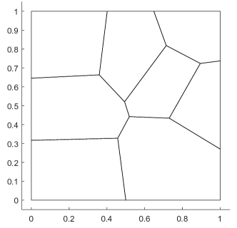
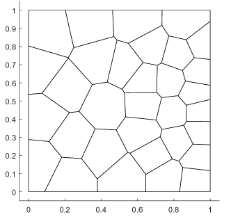
Figure 3: Examples of Voronoi meshes with $8$ and $32$ elements.

In Figure 4, we plot the computable quantity (105) obtained by employing $p=2q+1$ plane waves in the definition of the local spaces $\mathbb{PW}_{p}(K)$ in (11), with $q=4$ and 7, against the inverse of the product $hk$. We tested the method for different wave numbers $k$.

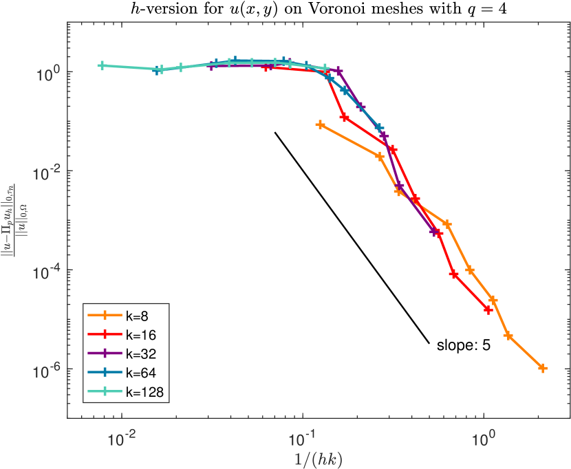
Figure 4: $h$-convergence of the nonconforming Trefftz-VEM on the Voronoi-Lloyd meshes for different values of the wave number $k$. The computable quantity (105) is plotted against the inverse of the product $hk$. Local spaces with $p=9$ (left) and $p=15$ (right) plane waves are used.

Firstly, we notice that the error curves are not precisely straight; this is due to the fact that the Voronoi meshes (even after some Lloyd iterations) contain elements with substantially different size. We remark that similar tests on Cartesian meshes led to straight lines. Moreover, the decreasing behavior stops once the product $hk$ becomes “too small”, as compared to $p$; this can be traced back to the ill-conditioning of the plane wave basis (similar results are obtained employing plane wave-discontinuous Galerkin methods, see [25]). The tests indicate algebraic convergence rate of order $\mathcal{O}((hk)^{q+1})$ (see also Figure 5) and, as typical of plane wave based methods, a delayed onset of convergence for higher values of $k$.

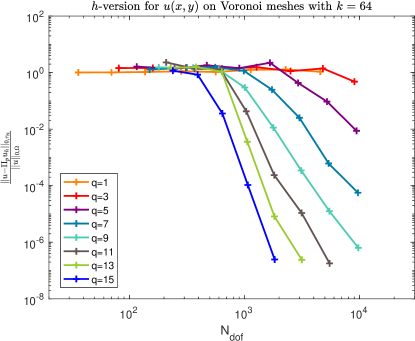
Figure 5: $h$-convergence of the nonconforming Trefftz-VEM on the Voronoi-Lloyd meshes for different values of $q$ and fixed wave number $k=64$. The computable quantity (105) is plotted against the number of degrees of freedom.

6 Conclusions

In the present work, we have introduced a nonconforming Trefftz virtual element method based on polygonal grids for the two dimensional Helmholtz problem. We do not hereby use fully discontinuous trial and test functions, but rather the jumps across interfaces are imposed to zero in a nonconforming sense. In addition, local spaces are Trefftz, which implies that less degrees of freedom are needed for reaching a certain accuracy, as compared to standard polynomial based methods. The definition of the nonconforming Trefftz-VEM requires computable projectors, which map functions in the local approximation spaces into plane wave spaces, and computable stabilizations, which guarantee a discrete Gårding inequality. Importantly, only degrees of freedom on the mesh interfaces are used.

The construction of nonconforming Trefftz-VE spaces is based on the following strategy, which generalizes that of nonconforming harmonic VE spaces of [18], and which we deem can be extended to other (linear) settings:

1. on each element $K\in\mathcal{T}_{n}$, one introduces local discrete spaces $V_{h}(K)$ made of implicitly defined functions in the kernel of the target differential operator and whose traces on each element edge are defined such that $V_{h}(K)$ contains a finite dimensional space, say, $W(K)$, with good approximation properties and whose functions are available in closed form;

2. the degrees of freedom are defined so that the global trial and test spaces $V_{h}$ can be built in a nonconforming fashion, and so that the best approximation error for functions in $V_{h}$ is bounded by the best approximation error for functions in $\Pi_{K\in\mathcal{T}_{n}}W(K)$.

We underline that, differently from Trefftz discontinuous methods, the nonconforming Trefftz-VEM allows to recover information on the solution over the mesh skeleton, via edge projection operators. Moreover, differently from standard partition of unity methods, its construction neither requires explicit knowledge of basis functions nor quadrature formulas. The implementation of the nonconforming Trefftz-VEM is described in [34], together with an extensive discussion of its numerical performance, and a comparison with other methods in the literature.

References

- [1] M. Abramowitz and I. A. Stegun. Handbook of Mathematical Functions with Formulas, Graphs, and Mathematical Tables. 1964.
- [2] P. F. Antonietti, G. Manzini, and M. Verani. The fully nonconforming virtual element method for biharmonic problems. Math. Models Methods Appl. Sci., 28(02):387–407, 2018.
- [3] B. Ayuso, K. Lipnikov, and G. Manzini. The nonconforming virtual element method. ESAIM Math. Model. Numer. Anal., 50(3):879–904, 2016.
- [4] I. Babuška and J. M. Melenk. The partition of unity finite element method: basic theory and applications. Comput. Methods Appl. Mech. Engrg., 139(1-4):289–314, 1996.
- [5] R. Bañuelos and T. Carroll. Brownian motion and the fundamental frequency of a drum. Duke Math. J., 75(3):575–602, 1994.
- [6] L. Beirão da Veiga, F. Brezzi, A. Cangiani, G. Manzini, L.D. Marini, and A. Russo. Basic principles of virtual element methods. Math. Models Methods Appl. Sci., 23(01):199–214, 2013.
- [7] L. Beirão da Veiga, F. Brezzi, L.D. Marini, and A. Russo. The hitchhiker’s guide to the virtual element method. Math. Models Methods Appl. Sci., 24(8):1541–1573, 2014.
- [8] L. Beirão da Veiga, A. Chernov, L. Mascotto, and A. Russo. Basic principles of virtual elements on quasiuniform meshes. Math. Models Methods Appl. Sci., 26(8):1567–1598, 2016.
- [9] L. Beirão da Veiga, F. Dassi, and A. Russo. High-order virtual element method on polyhedral meshes. Comput. Math. Appl., 74(5):1110–1122, 2017.
- [10] L. Beirão da Veiga, C. Lovadina, and G. Vacca. Divergence free virtual elements for the Stokes problem on polygonal meshes. ESAIM Math. Model. Numer. Anal., 51(2):509–535, 2017.
- [11] M.F. Benedetto, S. Berrone, S. Pieraccini, and S. Scialò. The virtual element method for discrete fracture network simulations. Comput. Meth. Appl. Mech. Engrg., 280:135–156, 2014.
- [12] J. Bramble and L. Payne. Bounds in the Neumann problem for second order uniformly elliptic operators. Pac. J. Math., 12(3):823–833, 1962.
- [13] S. C. Brenner. Poincaré–Friedrichs inequalities for piecewise functions. SIAM J. Numer. Anal., 41(1):306–324, 2003.
- [14] S. C. Brenner and L.-Y.. Sung. Virtual element methods on meshes with small edges or faces. Math. Models Methods Appl. Sci., 268(07):1291–1336, 2018.
- [15] A. Cangiani, V. Gyrya, and G. Manzini. The nonconforming virtual element method for the Stokes equations. SIAM J. Numer. Anal., 54(6):3411–3435, 2016.
- [16] A. Cangiani, G. Manzini, and O. J. Sutton. Conforming and nonconforming virtual element methods for elliptic problems. IMA J. Numer. Anal., 37(3):1317–1354, 2016.
- [17] O. Cessenat and B. Despres. Application of an ultra weak variational formulation of elliptic PDEs to the two-dimensional Helmholtz problem. SIAM J. Numer. Anal., 35(1):255–299, 1998.
- [18] A. Chernov and L. Mascotto. The harmonic virtual element method: stabilization and exponential convergence for the Laplace problem on polygonal domains, 2018. doi: https://doi.org/10.1093/imanum/dry038.
- [19] E. Deckers, O. Atak, L. Coox, R. D’Amico, H. Devriendt, S. Jonckheere, K. Koo, B. Pluymers, D. Vandepitte, and W. Desmet. The wave based method: An overview of 15 years of research. Wave Motion, 51(4):550–565, 2014.
- [20] C. L. Epstein and M. O’Neil. Smoothed corners and scattered waves. SIAM J. Sci. Comput., 38(5):A2665–A2698, 2016.
- [21] L. C. Evans. Partial Differential Equations. American Mathematical Society, 2010.
- [22] C. Farhat, I. Harari, and L. P. Franca. The discontinuous enrichment method. Comput. Methods Appl. Mech. Engrg., 190(48):6455–6479, 2001.
- [23] E. Gagliardo. Caratterizzazioni delle tracce sulla frontiera relative ad alcune classi di funzioni in n variabili. Rend. Sem. Mat. Univ. Padova, 27(405):284–305, 1957.
- [24] F. Gardini, G. Manzini, and G. Vacca. The nonconforming virtual element method for eigenvalue problems. http://arxiv.org/abs/1802.02942, 2018.
- [25] C. J. Gittelson, R. Hiptmair, and I. Perugia. Plane wave discontinuous Galerkin methods: analysis of the -version. ESAIM Math. Model. Numer. Anal., 43(2):297–331, 2009.
- [26] R. Hiptmair, A. Moiola, and I Perugia. Plane wave approximation of homogeneous Helmholtz solutions. Z. Angew. Math. Phys., 62(5):809, 2011.
- [27] R. Hiptmair, A. Moiola, and I. Perugia. Plane wave discontinuous Galerkin methods for the 2D Helmholtz equation: analysis of the -version. SIAM J. Numer. Anal., 49(1):264–284, 2011.
- [28] R. Hiptmair, A. Moiola, and I. Perugia. A survey of Trefftz methods for the Helmholtz equation. In Building bridges: connections and challenges in modern approaches to numerical partial differential equations, pages 237–279. Springer, 2016.
- [29] J. Ladevèze and P. Ladevèze. Bounds of the Poincaré constant with respect to the problem of star-shaped membrane regions. Z. Angew. Math. Phys., 29(4):670–683, 1978.
- [30] X. Liu and Z. Chen. The nonconforming virtual element method for the Navier-Stokes equations. Adv. Comput. Math., 2018.
- [31] L. Mascotto. The version of the Virtual Element Method. PhD thesis, 2018.
- [32] L. Mascotto. Ill-conditioning in the virtual element method: stabilizations and bases. Numer. Methods Partial Differential Equations, 34(4):1258–1281, 2018.
- [33] L. Mascotto, I. Perugia, and A. Pichler. Non-conforming harmonic virtual element method: - and -versions, 2018. https://doi.org/10.1007/s10915-018-0797-4.
- [34] L. Mascotto, I. Perugia, and A. Pichler. A nonconforming Trefftz virtual element method for the Helmholtz problem: numerical aspects. https://arxiv.org/abs/1807.11237, 2018.
- [35] W. C. H. McLean. Strongly Elliptic Systems and Boundary Integral Equations. Cambridge University Press, 2000.
- [36] M. Melenk. On generalized Finite Element Methods. PhD thesis, University of Maryland, 1995.
- [37] A. Moiola. Trefftz-discontinuous Galerkin methods for time-harmonic wave problems. PhD thesis, ETH Zürich, 2011.
- [38] P. Monk and D.-Q. Wang. A least-squares method for the Helmholtz equation. Comput. Methods Appl. Mech. Engrg., 175(1-2):121–136, 1999.
- [39] D. Mora, G. Rivera, and R. Rodríguez. A virtual element method for the Steklov eigenvalue problem. Math. Models Methods Appl. Sci., 25(08):1421–1445, 2015.
- [40] L. E. Payne and H. F. Weinberger. An optimal Poincaré inequality for convex domains. Arch. Ration. Mech. Anal., 5(1):286–292, 1960.
- [41] I. Perugia, P. Pietra, and A. Russo. A plane wave virtual element method for the Helmholtz problem. ESAIM Math. Model. Numer. Anal., 50(3):783–808, 2016.
- [42] H. Riou, P. Ladeveze, and B. Sourcis. The multiscale VTCR approach applied to acoustics problems. J. Comput. Acoust., 16(04):487–505, 2008.
- [43] A. H. Schatz. An observation concerning Ritz-Galerkin methods with indefinite bilinear forms. Math. Comp., 28(128):959–962, 1974.
- [44] C. Talischi, G. H. Paulino, A. Pereira, and I. F. M. Menezes. PolyMesher: a general-purpose mesh generator for polygonal elements written in Matlab. Struct. Multidiscip. Optim., 45(3):309–328, 2012.
- [45] H. Triebel. Interpolation theory, function spaces, differential operators. North-Holland, 1978.
- [46] G. Vacca. An -conforming virtual element for Darcy and Brinkman equations. Math. Models Methods Appl. Sci., 28(01):159–194, 2018.
- [47] J. Zhao, S. Chen, and B. Zhang. The nonconforming virtual element method for plate bending problems. Math. Models Methods Appl. Sci., 26(09):1671–1687, 2016.