Some problems of arithmetic origin in rational dynamics

Abstract.

These are lecture notes from a course in arithmetic dynamics given in Grenoble in June 2017. The main purpose of this text is to explain how arithmetic equidistribution theory can be used in the dynamics of rational maps on $\mathbf{P}^{1}$. We first briefly introduce the basics of the iteration theory of rational maps on the projective line over $\mathbf{C}$, as well as some elements of iteration theory over an arbitrary complete valued field and the construction of dynamically defined height functions for rational functions defined over $\overline{\mathbf{Q}}$. The equidistribution of small points gives some original information on the distribution of preperiodic orbits, leading to some non-trivial rigidity statements. We then explain some consequences of arithmetic equidistribution to the study of the geometry of parameter spaces of such dynamical systems, notably pertaining to the distribution of special parameters and the classification of special subvarieties.

Introduction

In the recent years a number of classical ideas and problems in arithmetics have been transposed to the setting of rational dynamics in one and several variables. A main source of motivation in these developments is the analogy between torsion points on an Abelian variety and (pre-)periodic points of rational maps. This is actually more than an analogy since torsion points on an Abelian variety $A$ are precisely the preperiodic points of the endomorphism of $A$ induced by multiplication by 2. Thus, problems about the distribution or structure of torsion points can be translated to dynamical problems. This analogy also applies to spaces of such objects: in this way elliptic curves with complex multiplication would correspond to post-critically finite rational maps. Again one may ask whether results about the distribution of these “special points” do reflect each other. This point of view was in particular put forward by J. Silverman (see [39, 40] for a detailed presentation and references).

Our goal is to present a few recent results belonging to this line of research. More precisely we will concentrate on some results in which potential theory and arithmetic equidistribution, as presented in this volume by P. Autissier and A. Chambert-Loir (see [2, 11]), play a key role. This includes:

• an arithmetic proof of the equidistribution of periodic orbits towards the equilibrium measure as well as some consequences (Section 6);

• the equidistribution of post-critically finite mappings in the parameter space of degree 2 (Section 7) and degree $d\geq 3$ polynomials (Section 8);

• the classification of special curves in the space of cubic polynomials (Section 9).

A large part of these results is based on the work of Baker-DeMarco [4, 3] and Favre-Gauthier [21, 22].

These notes are based on a series of lectures given by the author in a summer school in Grenoble in June 2017, which were intended for an audience with minimal knowledge in complex analysis and dynamical systems. The style is deliberately informal and favors reading flow against precision, in order to arrive rather quickly at some recent advanced topics. In particular the proofs are mostly sketched, with an emphasis on the dynamical parts of the arguments. The material in Part I is standard and covered with much greater detail in classical textbooks: see e.g. Milnor [35] or Carleson-Gamelin [10] for holomorphic dynamics, and Silverman [39] for the arithmetic side. Silverman’s lecture notes [40] and DeMarco’s 2018 ICM address [13] contain similar but more advanced material.

Part I Basic holomorphic and arithmetic dynamics on ${\mathbf{P}^{1}}$

1. A few useful geometric tools

Uniformization

Theorem (Uniformization Theorem).

Every simply connected Riemann surface is biholomorphic to the open unit disk $\mathbf{D}$, the complex plane $\mathbf{C}$ or the Riemann sphere ${\mathbf{P}^{1}}(\mathbf{C})$.

See [14] for a beautiful and thorough treatment of this result and of its historical context. A Riemann surface $S$ is called hyperbolic (resp. parabolic) if its universal cover is the unit disk (resp. the complex plane). Note that in this terminology, an elliptic curve $E\simeq\mathbf{C}/\Lambda$ is parabolic. In a sense, “generic” Riemann surfaces are hyperbolic, however, interesting complex dynamics occurs only on parabolic Riemann surfaces or on ${\mathbf{P}^{1}}(\mathbf{C})$.

Theorem.

If $a$, $b$, $c$ are distinct points on ${\mathbf{P}^{1}}(\mathbf{C})$, then ${\mathbf{P}^{1}}(\mathbf{C})\setminus\left\{a,b,c\right\}$ is hyperbolic.

Proof.

Since the Möbius group acts transitively on triples of points, we may assume that $\left\{a,b,c\right\}=\left\{0,1,\infty\right\}$. Fix a base point $\star\in\mathbf{C}\setminus\left\{0,1\right\}$, then the fundamental group $\pi_{1}(\mathbf{C}\setminus\left\{0,1\right\},\star)$ is free on two generators. Let $S\to\mathbf{C}\setminus\left\{0,1\right\}$ be a universal cover. Since $\mathbf{C}\setminus\left\{0,1\right\}$ is non-compact, then $S$ is biholomorphic to $\mathbf{D}$ or $\mathbf{C}$. The deck transformation group is a group of automorphisms of $S$ acting discretely and isomorphic to the free group on two generators. The affine group $\mathrm{Aut}(\mathbf{C})$ has no free subgroups (since for instance its commutator subgroup is Abelian) so necessarily $S\simeq\mathbf{D}$. ∎

Corollary.

If $\Omega$ is an open subset of ${\mathbf{P}^{1}}(\mathbf{C})$ whose complement contains at least 3 points, then $\Omega$ is hyperbolic.

Recall that a family $\mathcal{F}$ of meromorphic functions on some open set $\Omega$ is said normal if it is equicontinuous w.r.t. the spherical metric, or equivalently, if it is relatively compact in the compact-open topology. Concretely, if $(f_{n})$ is a sequence in a normal family $\mathcal{F}$, then there exists a subsequence converging locally uniformly on $\Omega$ to a meromorphic function.

Theorem (Montel).

If $\Omega$ is an open subset of ${\mathbf{P}^{1}}(\mathbf{C})$ and $\mathcal{F}$ is a family of meromorphic functions in $\Omega$ avoiding 3 values, then $\mathcal{F}$ is normal.

Proof.

By post-composing with a Möbius transformation we may assume that $\mathcal{F}$ avoids $\left\{0,1,\infty\right\}$. Pick a disk $D\subset\Omega$ and a sequence $(f_{n})\in\mathcal{F}^{\mathbf{N}}$. It is enough to show that $(f_{n}\arrowvert_{D})$ is normal. A first possibility is that $(f_{n}\arrowvert_{D})$ diverges uniformly in $\mathbf{C}\setminus\left\{0,1\right\}$, that is is converges to $\left\{0,1,\infty\right\}$, and in this case we are done. Otherwise there exists $t_{0}\in D$, $z_{0}\in\Omega$ and a subsequence $(n_{j})$ such that $f_{n_{j}}(t_{0})\to z_{0}$. Then if $\psi:\mathbf{D}\to\mathbf{C}\setminus\left\{0,1\right\}$ is a universal cover such that $\psi(0)=z_{0}$, lifting $(f_{n_{j}})$ under $\psi$ yields a sequence $\hat{f}_{n_{j}}:D\to\mathbf{D}$ such that $\hat{f}_{n_{j}}(t_{0})\to 0$. The Cauchy estimates imply that $(\hat{f}_{n_{j}})$ is locally uniformly Lipschitz in $D$ so by the Ascoli-Arzela theorem, extracting further if necessary, $(\hat{f}_{n_{j}})$ converges to some $\hat{f}:D\to\mathbf{D}$. Finally, $f_{n_{j}}$ converges to $\psi\circ\hat{f}$ and we are done. ∎

The hyperbolic metric

First recall the Schwarz-Lemma: if $f:\mathbf{D}\to\mathbf{D}$ is a holomorphic map such that $f(0)=0$, then $\left|f^{\prime}(0)\right|\leq 1$, with equality if and only if $f$ is an automorphism, which must then be a rotation.

More generally, any automorphism of $\mathbf{D}$ is of the form $f(z)=e^{i\theta}\frac{z-\alpha}{1-\bar{\alpha}z}$, for some $\theta\in\mathbf{R}$ and $\left|\alpha\right|<1$, and the inequality in the Schwarz Lemma can then be propagated as follows: let $\rho$ be the Riemannian metric on $\mathbf{D}$ defined by the formula $\rho(z)=\frac{2\left|dz\right|}{1-\left|z\right|^{2}}$, i.e. if $v$ is a tangent vector at $z$, $v\in T_{z}\mathbf{D}\simeq\mathbf{C}$, then $\left\|v\right\|_{\rho}=\frac{2\left|v\right|}{1-\left|z\right|^{2}}$. This metric is referred to as the hyperbolic (or Poincaré) metric and the Riemannian manifold $(\mathbf{D},\rho)$ is the hyperbolic disk.

Theorem (Schwarz-Pick Lemma).

Any holomorphic map $f:\mathbf{D}\to\mathbf{D}$ is a weak contraction for the hyperbolic metric. It is a strict contraction unless $f$ is an automorphism.

If now $S$ is any hyperbolic Riemann surface, since the deck transformation group of the universal cover $\mathbf{D}\to S$ acts by isometries, we can push $\rho$ to a well-defined hyperbolic metric on $S$. As before any holomorphic map $f:S\to S^{\prime}$ between hyperbolic Riemann surfaces is a weak contraction, and it is a strict contraction unless $f$ lifts to an isometry between their universal covers.

2. Review of rational dynamics on ${\mathbf{P}^{1}}(\mathbf{C})$

Let $f:{\mathbf{P}^{1}}(\mathbf{C})\to{\mathbf{P}^{1}}(\mathbf{C})$ be a rational map of degree $d$, that is $f$ can be written in homogeneous coordinates as $[P(z,w):Q(z,w)]$, where $P$ and $Q$ are homogeneous polynomials of degree $d$ without common factors. Equivalently, $f(z)=\frac{P(z)}{Q(z)}$ in some affine chart. It is an elementary fact that any holomorphic self-map on ${\mathbf{P}^{1}}(\mathbf{C})$ is rational. In particular the group of automorphisms of ${\mathbf{P}^{1}}(\mathbf{C})$ is the Möbius group $\mathrm{PGL}(2,\mathbf{C})$.

We consider $f$ as a dynamical system, that is we wish to understand the asymptotic behavior of the iterates $f\circ\cdots\circ f=:f^{n}$. General references for the results of this section include [35, 10]. Throughout these notes, we make the standing assumption that $d\geq 2$.

Fatou-Julia dichotomy

The Fatou set $F(f)$ is the set of points $z\in{\mathbf{P}^{1}}(\mathbf{C})$ such that there exists a neighborhood $N\ni z$ on which the sequence of iterates $(f^{n}\arrowvert_{N})$ is normal. It is open by definition. A typical situation occurring in the Fatou set is that of an attracting orbit: that is an invariant finite set $A$ such that every nearby point converges under iteration to $A$. The locus of non-normality or Julia set $J(f)$ is the complement of the Fatou set: $J(f)=F(f)^{\complement}$. When there is no danger of confusion we feel free to drop the dependence on $f$.

The Fatou and Julia sets are invariant ($f(X)\subset X$, where $X=F(f)$ or $J(f)$) and even totally invariant ($f^{-1}(X)=X$). Since $d\geq 2$ it easily follows that $J(f)$ is nonempty. On the other hand the Fatou set may be empty.

If $z\in J(f)$ and $N$ is a neighborhood of $z$, it follows from Montel’s theorem that $\bigcup_{n\geq 0}f^{n}(N)$ avoids at most 2 points. Define

$$E_{z}=\bigcap_{N\ni z}\left({\mathbf{P}^{1}}(\mathbf{C})\setminus\bigcup_{n\geq 0}f^{n}(N)\right).$$

Proposition 2.1.

The set $E:=E_{z}$ is independent of $z\in J(f)$. Its cardinality is at most 2 and it is the maximal totally invariant finite subset. Furthermore:

• If $\#E=1$ then $f$ is conjugate in $\mathrm{PGL}(2,\mathbf{C})$ to a polynomial.

• If $\#E=2$ then $f$ is conjugate in $\mathrm{PGL}(2,\mathbf{C})$ to $z\mapsto z^{\pm d}$.

The set $E(f)$ is called the exceptional set of $f$. Note that it is always an attracting periodic orbit, in particular it is contained in the Fatou set.

Proof.

It is immediate that $f^{-1}(E_{z})\subset E_{z}$ and by Montel’s Theorem $\#E_{z}\leq 2$. If $\#E_{z}=1$, then we may conjugate so that $E_{z}=\left\{\infty\right\}$ and since $f^{-1}(\infty)=\infty$ it follows that $f$ is a polynomial. If $\#E_{z}=2$ we conjugate so that $E_{z}=\left\{0,\infty\right\}$. If both points are fixed then it is easy to see that $f(z)=z^{d}$, and in the last case that $f(z)=z^{-d}$. The independence with respect to $z$ follows easily. ∎

The following is an immediate consequence of the definition of $E$.

Corollary 2.2.

For every $z\notin E$, $\displaystyle\overline{\bigcup\nolimits_{n\geq 0}f^{-n}(z)}\supset J$.

Let us also note the following consequence of Montel’s Theorem.

Corollary 2.3.

If the Julia set $J$ has non-empty interior, then $J={\mathbf{P}^{1}}(\mathbf{C})$.

What does $J(f)$ look like?

The Julia set is closed, invariant, and infinite (apply Corollary 2.2 to $z\in J$). It can be shown that $J$ is perfect (i.e. has no isolated points).

A first possibility is that $J$ is the whole sphere ${\mathbf{P}^{1}}(\mathbf{C})$. It is a deep result by M. Rees [37] that this occurs with positive probability if a rational map is chosen at random in the space of all rational maps of a given degree. Note that this never happens for polynomials because $\infty$ is an attracting point.

Important explicit examples of rational maps with $J={\mathbf{P}^{1}}$ are Lattès mappings, which are rational maps coming from multiplication on an elliptic curve. In a nutshell: let $E$ be an elliptic curve, viewed as a torus $\mathbf{C}/\Lambda$, where $\Lambda$ is a lattice, and let $m:\mathbf{C}\to\mathbf{C}$ be a $\mathbf{C}$-linear map such that $m(\Lambda)\subset\Lambda$. Then $m$ commutes with the involution $z\mapsto-z$, so it descends to a self-map of the quotient Riemann surface $E/(z\sim(-z))$ which turns out to be ${\mathbf{P}^{1}}(\mathbf{C})$. The calculations can be worked out explicitly for the doubling map using elementary properties of the Weierstraß $\wp$-function, and one finds for instance that $f(z)=\frac{(z^{2}+1)^{2}}{4z(z^{2}-1)}$ is a Lattès example (see e.g. [36] for this and more about Lattès mappings).

It can also happen that $J$ is a smooth curve (say of class $C^{1}$). A classical theorem of Fatou then asserts that $J$ must be contained in a circle (this includes lines in $\mathbf{C}$), and more precisely:

• either it is a circle: this happens for $z\mapsto z^{\pm d}$ but also for some Blaschke products;

• or it is an interval in a circle: this happens for interval maps such as the Chebychev polynomial $z\mapsto z^{2}-2$ for which $J=[-2,2]$.

Otherwise $J$ is a self-similar “fractal” set with often complicated topological structure (see Figure 1).

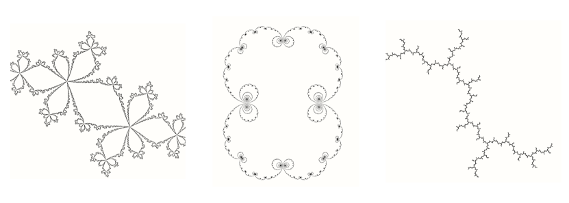
Figure 1. Gallery of quadratic Julia sets $J(f_{c})$ with $f_{c}(z)=z^{2}+c$. Left: $z^{2}+(-.5+.556i)$, middle: $z^{2}+.2531$, right: $z^{2}+i$.

Periodic points

A point $z\in{\mathbf{P}^{1}}(\mathbf{C})$ is periodic if there exists $n$ such that $f^{n}(z)=z$. The period of $z$ is the minimal such positive $n$, And a fixed point is a point of period 1. Elementary algebra shows that $f^{n}$ admits $d^{n}+1$ fixed points counting multiplicities. If $z_{0}$ has exact period $n$, the multiplier of $z_{0}$ is the complex number $(f^{n})^{\prime}(z_{0})$ (which does not depend on the chosen Riemannian metric on the sphere). It determines a lot of the local dynamics of $f^{n}$ near $z_{0}$. There are three main cases:

• attracting: $\left|(f^{n})^{\prime}(z_{0})\right|<1$: then $z_{0}\in F$ and for $z$ near $z_{0}$, $f^{nk}(z)\to z_{0}$ as $k\to\infty$;

• repelling: $\left|(f^{n})^{\prime}(z_{0})\right|>1$: then $z_{0}\in J$ since $\left|(f^{nk})^{\prime}(z_{0})\right|\to\infty$ as $k\to\infty$;

• neutral: $\left|(f^{n})^{\prime}(z_{0})\right|=1$: then $z_{0}$ belongs to either $F$ or $J$.

The neutral case subdivides further into rationally neutral (or parabolic) when $(f^{n})^{\prime}(z_{0})$ is a root of unity and irrationally neutral otherwise. Parabolic points belong to the Julia set. The dynamical classification of irrationally neutral points, which essentially boils down to the question whether they belong to the Fatou or Julia set, is quite delicate (and actually still not complete) and we will not need it.

Theorem 2.4 (Fatou, Julia).

Repelling periodic points are dense in $J(f)$.

This is an explanation for the local self-similarity of $J$. In particular we see that if $z_{0}$ is repelling with a non-real multiplier, then $J$ has a “spiralling structure” at $z_{0}$, in particular it cannot be smooth. A delicate result by Eremenko and Van Strien [20] asserts conversely that if all periodic points multipliers are real, then $J$ is contained in a circle.

Idea of proof.

The first observation is that if $g$ is a holomorphic self-map of an open topological disk $\Delta$ such that $\overline{g(\Delta)}\subset\Delta$, then by contraction of the Poincaré metric, $g$ must have an attracting fixed point. If now $z_{0}\in J$ is arbitrary we know from Montel’s Theorem and the classification of exceptional points that for any neighborhood $N\ni z_{0}$, $\bigcup_{n\geq 0}f^{n}(N)$ eventually covers $J$, hence $z_{0}$. With some more work, it can be ensured that there exists a small open disk $D$ close to $z_{0}$ and an integer $n$ such that $f^{n}$ is univalent on $D$ and $\overline{D}\subset f^{n}(D)$. Then the result follows from the initial observation. ∎

In particular a rational map admits infinitely many repelling points. It turns out that conversely the number of non-repelling periodic points is finite. The first step is the following basic result.

Theorem 2.5 (Fatou).

Every attracting periodic orbit attracts a critical point.

By this mean that for every attracting periodic orbit $A$ there exists a critical point $c$ such that $f^{n}(c)$ tends to $A$ as $n\to\infty$. This is a basic instance of a general heuristic principle: the dynamics is determined by the behavior of critical points.

Proof.

Let $z_{0}$ be an attracting point of period $n$. For expositional ease we replace $f$ by $f^{n}$ so assume $n=1$. Let

$$\mathcal{B}=\left\{z\in{\mathbf{P}^{1}},\ f^{k}(z)\underset{k\to\infty}{\longrightarrow}z_{0}\right\}$$

be the basin of $z_{0}$ and $\mathcal{B}_{0}$ be the immediate basin, that is the connected component of $z_{0}$ in $\mathcal{B}$. Then $f$ maps $\mathcal{B}_{0}$ into itself and $\mathcal{B}_{0}$ is hyperbolic since $\mathcal{B}_{0}\cap J=\emptyset$. If $f\arrowvert_{\mathcal{B}_{0}}$ had no critical points, then $f\arrowvert_{\mathcal{B}_{0}}$ would be a covering, hence a local isometry for the hyperbolic metric. This contradicts the fact that $z_{0}$ is attracting. ∎

Since $f$ has $2d-2$ critical points we infer:

Corollary 2.6.

A rational map of degree $d$ admits at most $2d-2$ attracting periodic orbits.

Theorem 2.7 (Fatou, Shishikura).

A rational map admits only finitely many non-repelling periodic orbits.

Idea of proof.

The bound $6d-6$ was first obtained by Fatou by a beautiful perturbative argument. First, the previous theorem (and its corollary) can be easily extended to the case of periodic orbits with multiplier equal to 1 (these are attracting in a certain direction). So there are at most $2d-2$ periodic points with multiplier 1. Let now $N$ be the number of neutral periodic points with multiplier different from 1. Fatou shows that under a generic perturbation of $f$, at least half of them become attracting. Hence $N/2\leq 2d-2$ and the result follows.

The sharp bound $2d-2$ for the total number of non-repelling cycles was obtained by Shishikura. ∎

Fatou dynamics

The dynamics in the Fatou set can be understood completely. Albeit natural, this is far from obvious: one can easily imagine an open set $U$ on which the iterates form a normal family, yet the asymptotic behavior of $(f^{n}\arrowvert_{U})$ is complicated to analyze. Such a phenomenon actually happens in transcendental or higher dimensional dynamics, but not in our setting: the key point is the following deep and celebrated “non-wandering domain theorem”.

Theorem 2.8 (Sullivan).

Every component $U$ of the Fatou set is ultimately periodic, i.e. there exist integers $l>k$ such that $f^{l}(U)=f^{k}(U)$.

It remains to classify periodic components.

Theorem 2.9.

Every component $U$ of period $k$ of the Fatou set is

• either an attraction domain: as $n\to\infty$, $(f^{nk})$ converges locally uniformly on $U$ to a periodic cycle (attracting or parabolic);

• or a rotation domain: $U$ is biholomorphic to a disk or an annulus and $f^{k}\arrowvert_{U}$ is holomorphically conjugate to an irrational rotation.

3. Equilibrium measure

In many arithmetic applications the most important dynamical object is the equilibrium measure. The following theorem summarizes its construction and main properties.

Theorem 3.1 (Brolin, Lyubich, Freire-Lopes-Mañé).

Let $f$ be a rational map on ${\mathbf{P}^{1}}(\mathbf{C})$ of degree $d\geq 2$. Then for any $z\notin E(f)$, the sequence of probability measures

$$\mu_{n,z}=\frac{1}{d^{n}}\sum_{w\in f^{-n}(z)}\delta_{w}$$

(where pre-images are counted with their multiplicity) converges weakly to a Borel probability measure $\mu=\mu_{f}$ on ${\mathbf{P}^{1}}(\mathbf{C})$ enjoying the following properties:

1. $\mu$ is invariant, that is $f_{*}\mu=\mu$, and has the “constant Jacobian” property $f^{*}\mu=d\mu$;

2. $\mu$ is ergodic;

3. $\operatorname{Supp}(\mu)=J(f)$;

4. $\mu$ is repelling, that is for $\mu$-a.e. $z$, $\displaystyle\liminf_{n\to\infty}\frac{1}{n}\log\left\|df^{n}_{z}\right\|\geq\frac{\log d}{2}$, where the norm of the differential is computed with respect to any smooth Riemannian metric on ${\mathbf{P}^{1}}(\mathbf{C})$;

5. $\mu$ describes the asymptotic distribution of repelling periodic orbits, that is, if $\mathrm{RPer}_{n}$ denotes the set of repelling periodic points of exact period $n$, then $\frac{1}{d^{n}}\sum_{z\in\mathrm{RPer}_{n}}\delta_{z}$ converges to $\mu$ as $n\to\infty$.

Recall that if $\mu$ is a probability measure, its image $f_{*}\mu$ under $f$ is defined by $f_{*}\mu(A)=\mu(f^{-1}(A))$ for any Borel set $A$. The pull-back $f^{*}\mu$ is conveniently defined by its action on continuous functions: $\langle f^{*}\mu,\varphi\rangle=\langle\mu,f_{*}\varphi\rangle$, where $f_{*}\varphi$ is defined by $f_{*}\varphi(x)=\sum_{y\in f^{-1}(x)}\varphi(y)$. Recall also that ergodicity means that any measurable invariant subset has measure 0 or 1. A stronger form of ergodicity actually holds: $\mu$ is exact, that is, if $A$ is any measurable subset of positive measure, then $\mu(f^{n}(A))\to 1$ as $n\to\infty$.

The proof of this theorem is too long to be explained in these notes (see [26] for a detailed treatment). Let us only discuss the convergence statement.

Proof of the convergence of the $\mu_{n,z}$.

Consider the Fubini-Study $(1,1)$ form $\omega$ associated to the spherical metric on ${\mathbf{P}^{1}}$. It expresses in coordinates as $\omega=\frac{i}{\pi}\partial\overline{\partial}\log\left\|\sigma\right\|^{2}$ where $\sigma:{\mathbf{P}^{1}}\to{\mathbf{C}^{2}}\setminus\left\{0\right\}$ is any local section of the canonical projection ${\mathbf{C}^{2}}\setminus\left\{0\right\}\to{\mathbf{P}^{1}}$ and $\left\|\cdot\right\|$ is the standard Hermitian norm on ${\mathbf{C}^{2}}$, i.e $\left\|(z,w)\right\|^{2}=\left|z\right|^{2}+\left|w\right|^{2}$. Then

$$f^{*}\omega-d\omega=\frac{i}{\pi}\partial\overline{\partial}\log\frac{\left\|\left(P(z,w),Q(z,w)\right)\right\|^{2}}{\left\|(z,w)\right\|^{2d}}=:\frac{i}{\pi}\partial\overline{\partial}g_{0},$$

where by homogeneity of the polynomials $P$ and $Q$, $g_{0}$ is a globally well-defined smooth function on ${\mathbf{P}^{1}}$. Thus we infer that

$$\frac{1}{d^{n}}(f^{n})^{*}\omega-\omega =\sum_{k=0}^{n-1}\left(\frac{1}{d^{k+1}}(f^{k+1})^{*}\omega-\frac{1}{d^{k}}(f^{k})^{*}\omega\right)$$

$$=\sum_{k=0}^{n-1}\frac{1}{d^{k+1}}(f^{k})^{*}(f^{*}\omega-d\omega)$$

$$=\frac{i}{\pi}\partial\overline{\partial}\left(\sum_{k=0}^{n-1}\frac{1}{d^{k+1}}g_{0}\circ f^{k}\right)=:\frac{i}{\pi}\partial\overline{\partial}g_{k}.$$

One readily sees that the sequence of functions $g_{k}$ converges uniformly to a continuous function $g_{\infty}$, therefore basic distributional calculus implies that

$$\frac{1}{d^{n}}(f^{n})^{*}\omega\underset{n\to\infty}{\longrightarrow}\omega+\frac{i}{\pi}\partial\overline{\partial}g_{\infty}.$$

Being a limit in the sense of distributions of a sequence of probability measures, this last term can be identified to a positive measure $\mu$ by declaring that

$$\langle\mu,\varphi\rangle=\int_{{\mathbf{P}^{1}}}\varphi\,\omega+\frac{i}{\pi}\int_{\pi}g_{\infty}\,\partial\overline{\partial}\varphi$$

for any smooth function $\varphi$. By definition this measure is the equilibrium measure $\mu_{f}$.

Now for any $z\in{\mathbf{P}^{1}}$, identifying (1,1) forms and signed measures as above we write

$$\frac{1}{d^{n}}\sum_{w\in f^{-n}(z)}\delta_{w}=\frac{1}{d^{n}}(f^{n})^{*}\delta_{z}=\frac{1}{d^{n}}(f^{n})^{*}\omega+\frac{1}{d^{n}}(f^{n})^{*}(\delta_{z}-\omega).$$

There exists a $L^{1}$ function on ${\mathbf{P}^{1}}$ such that in the sense of distributions $\frac{i}{\pi}\partial\overline{\partial}g_{z}=\delta_{z}-\omega$, so that

$$\frac{1}{d^{n}}(f^{n})^{*}(\delta_{z}-\omega)=\frac{i}{\pi}\partial\overline{\partial}\left(\frac{1}{d^{n}}g_{z}\circ f^{n}\right)$$

and to establish the convergence of the $\mu_{n,z}$ the problem is to show that for $z\notin E$, ${d^{-n}}g_{z}\circ f^{n}$ converges to 0 in $L^{1}$. It is rather easy to prove that this convergence holds for a.e. $z$ with respect to Lebesgue measure. Indeed, suppose that the $g_{z}$ are chosen with some uniformity, for instance by assuming $\sup_{{\mathbf{P}^{1}}}{g_{z}}=0$. In this case the average $\int g_{z}\mathrm{Leb}(dz)$ is a bounded function $g$ (such that $\frac{i}{\pi}\partial\overline{\partial}g=\mathrm{Leb}$) and the result essentially follows from the Borel-Cantelli Lemma: indeed, on average, ${d^{-n}}g_{z}\circ f^{n}$ is bounded by ${C}^{st}/d^{n}$.

Proving the convergence for every $z\notin E$ requires a finer analysis, see [26] for details. ∎

The case of polynomials

If $f$ is a polynomial, rather than the Fubini-Study measure, we can use the Dirac mass at the totally invariant point $\infty$, to give another formulation of these results. Indeed, if $\nu$ is any probability measure (say with compact support) in $\mathbf{C}$, write $\nu-\delta_{\infty}=\frac{i}{\pi}\partial\overline{\partial}g$ as before. In $\mathbf{C}$, this rewrites as $\nu=\Delta g$, where $g$ is a subharmonic function with logarithmic growth at infinity: $g(z)=\log\left|z\right|+c+o(1)$. If $\nu_{S^{1}}$ be the normalized Lebesgue measure on the unit circle, then $\nu_{S^{1}}=\Delta\left(\log^{+}\left|z\right|\right)$ (where $\log^{+}t=\max(\log t,0)$), so

$$\frac{1}{d^{n}}(f^{n})^{*}(\nu_{S^{1}})=\frac{1}{d^{n}}\Delta\left(\log^{+}\left|f^{n}(z)\right|\right).$$

An argument similar to that of the proof of Theorem 3.1 yields the following:

Proposition 3.2.

If $f$ is a polynomial of degree $d$, the sequence of functions $d^{-n}\log^{+}\left|f^{n}\right|$ converges locally uniformly to a subharmonic function $G:\mathbf{C}\to\mathbf{R}$ satisfying $G\circ f=dG$.

The function $G=G_{f}$ is by definition the dynamical Green function of $f$. Introduce the filled Julia set

$$K(f) =\left\{z\in\mathbf{C},\ (f^{n}(z))\text{ is bounded in }\mathbf{C}\right\}$$

$$=\left\{z\in\mathbf{C},\ (f^{n}(z))\text{ does not tend to }\infty\right\}.$$

It is easy to show that $J(f)=\partial K(f)$.

Proposition 3.3.

The dynamical Green function has the following properties:

1. $G_{f}$ is continuous, non-negative and subharmonic in $\mathbf{C}$;

2. $\left\{G_{f}=0\right\}=K(f)$;

3. $\Delta G_{f}=\mu_{f}$ is the equilibrium measure (in particular $\operatorname{Supp}(\Delta G_{f})=\partial\left\{G_{f}=0\right\}$);

4. if $f$ is a monic polynomial, then $G_{f}(z)=\log\left|z\right|+o(1)$ as $z\to\infty$.

Properties (i)-(iii) show that the dynamically defined function $G_{f}$ coincides with the Green function of $K(f)$ from classical potential theory. Property (iv) implies that if $f$ is monic, then $K(f)$ is of capacity 1, which is important in view of its number-theoretic properties (see the lectures by P. Autissier in this volume [2]).

Another useful consequence is that the Green function $G_{f}$ is completely determined by the compact set $K(f)$ (or by its boundary $J(f)$). In particular if $f$ and $g$ are polynomials of degree at least 2 then

$$J(f)=J(g)\Leftrightarrow\mu_{f}=\mu_{g}.$$ (1)

The same is not true for rational maps: $J(f)$ does not determine $\mu_{f}$ in general. For instance there are many rational maps $f$ such that $J={\mathbf{P}^{1}}(\mathbf{C})$, however Zdunik [42] proved that $\mu_{f}$ is absolutely continuous with respect to the Lebesgue measure on ${\mathbf{P}^{1}}(\mathbf{C})$ (in this case automatically $J(f)={\mathbf{P}^{1}}(\mathbf{C})$) if and only if $f$ is a Lattès example.

4. Non-Archimedean dynamical Green function

Dynamics of rational functions over non-Archimedean valued fields has been developing rapidly during the past 20 years, greatly inspired by the analogy with holomorphic dynamics. Most of the results of the previous section have analogues in the non-Archimedean setting. We will not dwell upon the details in these notes, and rather refer the interested reader to [39, 5]. We shall content ourselves with recalling the vocabulary of valued fields and heights, and the construction of the dynamical Green function.

Vocabulary of valued fields

To fix notation and terminology let us first recall a few standard notions and facts.

Definition 4.1.

An absolute value $\left|\cdot\right|$ on a field $K$ is a function $K\to\mathbf{R}^{+}$ such that

• for every $\alpha\in K$, $\left|\alpha\right|\geq 0$ and $\left|\alpha\right|=0$ iff $\alpha=0$;

• for all $\alpha$, $\beta$, $\left|\alpha\beta\right|=\left|\alpha\right|\cdot\left|\beta\right|$;

• for all $\alpha$, $\beta$, $\left|\alpha+\beta\right|\leq\left|\alpha\right|+\left|\beta\right|$.

If in addition $\left|\cdot\right|$ satisfies the ultrametric triangle inequality $\left|\alpha+\beta\right|\leq\max(\left|\alpha\right|,\left|\beta\right|)$, then it is said non-Archimedean.

Besides the usual modulus on $\mathbf{C}$, a basic example is the $p$-adic norm on $\mathbf{Q}$, defined by $\left|\alpha\right|_{p}=p^{-v_{p}(\alpha)}$ where $v_{p}$ is the $p$-adic valuation: $v_{p}(a/b)=\ell$ where $a/b=p^{\ell}(a^{\prime}/b^{\prime})$ and $p$ does not divide $a^{\prime}$ nor $b^{\prime}$. On any field we can define the trivial absolute value by $\left|0\right|=0$ and $\left|x\right|=1$ if $x\neq 0$.

If $(K,\left|\cdot\right|)$ is a non-Archimedean valued field, we define the spherical metric on $\mathbf{P}^{1}(K)$ by

$$\rho(p_{1},p_{2})=\frac{\left|x_{1}y_{2}-x_{2}y_{1}\right|}{\max(\left|x_{1}\right|,\left|y_{1}\right|)\max(\left|x_{2}\right|,\left|y_{2}\right|)},$$

where $p_{1}=[x_{1}:y_{1}]$ and $p_{2}=[x_{2}:y_{2}]$. From the ultrametric inequality we infer that the $\rho$-diameter of $\mathbf{P}^{1}(K)$ equals 1.

Definition 4.2.

Two absolute values $\left|\cdot\right|_{1}$ and $\left|\cdot\right|_{2}$ on $K$ are said equivalent if there exists a positive real number $r$ such that $\left|\cdot\right|_{1}=\left|\cdot\right|_{2}^{r}$.

An equivalence class of absolute values on $K$ is called a place. The set of places of $K$ is denoted by $\mathcal{M}_{K}$.

Theorem 4.3 (Ostrowski).

A set of representatives of the set of places of $\mathbf{Q}$ is given by

• the trivial absolute value;

• the usual Archimedean absolute value $\left|\cdot\right|_{\infty}$;

• the set of $p$-adic absolute values $\left|\cdot\right|_{p}$.

Decomposition into prime factors yields the product formula

$$\forall x\in\mathbf{Q}^{*},\ \prod_{p\in\mathcal{P}\cup\left\{\infty\right\}}\left|x\right|_{p}=1,$$

where $\mathcal{P}$ denotes the set of prime numbers.

For number fields, places can also be described. First one considers $\mathbf{Q}_{p}$ the completion of $\mathbf{Q}$ relative to the distance induced by $\left|\cdot\right|_{p}$. The $p$-adic absolute value extends to an algebraic closure of $\mathbf{Q}_{p}$, so we may consider $\mathbf{C}_{p}$ the completion of this algebraic closure. (For $p=\infty$ of course $\mathbf{C}_{p}=\mathbf{C}$.)

A number field $K$ admits a number of embeddings $\sigma:K\hookrightarrow\mathbf{C}_{p}$, which define by restriction a family of absolute values $a\mapsto\left|\sigma(a)\right|_{p}$ on $K$. Distinct embeddings may induce the same absolute value. For any non-trivial absolute value $\left|\cdot\right|_{v}$ on $K$ there exists $p_{v}\in\mathcal{P}\cup\left\{\infty\right\}$ such that $\left|\cdot\right|_{v}\arrowvert_{\mathbf{Q}}$ is equivalent to $\left|\cdot\right|_{p_{v}}$ and $\varepsilon_{v}$ distinct embeddings $\sigma:K\hookrightarrow\mathbf{C}_{p_{v}}$ such that the restriction of $\left|\cdot\right|_{\mathbf{C}_{p_{v}}}$ to ${\sigma(K)}$ induces $\left|\cdot\right|_{v}$ up to equivalence. Thus for each place of $K$ we can define an absolute value $\left|\cdot\right|_{v}$ on $K$ that is induced by $\left|\cdot\right|_{\mathbf{C}_{p_{v}}}$ by embedding $K$ in $\mathbf{C}_{p_{v}}$ and the following product formula holds

$$\forall x\in K^{*},\ \prod_{v\in\mathcal{M}_{K}}\left|x\right|_{v}^{\varepsilon_{v}}=\prod_{p\in\mathcal{P}\cup\left\{\infty\right\}}\prod_{\sigma:K\hookrightarrow\mathbf{C}_{p}}\left|\sigma(x)\right|_{p}=1.$$ (2)

A similar formalism holds for certain non-algebraic extensions of $\mathbf{Q}$, giving rise to a general notion of product formula field.

Dynamical Green function

Let $(K,\left|\cdot\right|)$ be a complete valued field. If $f$ is a rational map on $\mathbf{P}^{1}(K)$ we can define a dynamical Green function as before, by working with homogeneous lifts to $\mathbf{A}^{2}(K)$. For $(x,y)\in\mathbf{A}^{2}(K)$ we put $\left\|(x,y)\right\|=\max(\left|x\right|,\left|y\right|)$, and fix a lift $F:\mathbf{A}^{2}(K)\to\mathbf{A}^{2}(K)$ of $f$.

Theorem 4.4.

For every $(x,y)\in\mathbf{A}^{2}(K)$, the limit

$$G_{F}(x,y):=\lim_{n\to\infty}\frac{1}{d^{n}}\log\left\|F^{n}(x,y)\right\|$$

exists.

The function $G_{F}$ is continuous on $\mathbf{A}^{2}(K)$ (relative to the norm topology) and satisfies

• $G_{F}\circ F=dG_{F}$;

• $G_{F}(x,y)=\log{\left\|(x,y)\right\|}+O(1)$ at infinity;

• $G_{F}(\lambda x,\lambda y)=\log\left|\lambda\right|+G_{F}(x,y)$.

Note that the function $G_{F}$ depends on the chosen lift, more precisely $G_{\alpha F}=\frac{1}{d-1}\log\left|\alpha\right|+G_{F}$. The proof of the theorem is similar to that of the Archimedean case. The key point is that there exists positive numbers $c_{1}$ and $c_{2}$ such that the inequality

$$c_{1}\leq\frac{\left\|F(x,y)\right\|}{\left\|(x,y)\right\|^{d}}\leq c_{2}$$ (3)

holds. The upper bound in (3) is obvious, and the lower bound is a consequence of the Nullstellensatz.

What is more delicate is to make sense of the measure theoretic part, i.e. to give a meaning to $\Delta G$. For this one has to introduce the formalism of Berkovich spaces, which is well-suited to measure theory (see [39, 5] for details).

If $f$ is a polynomial, instead of lifting to $\mathbf{A}^{2}$, we can directly consider the Green function on $K$ as in the complex case. More precisely: if $f$ is a polynomial of degree $d$, the sequence of functions $d^{-n}\log^{+}\left|f^{n}\right|$ converges locally uniformly to a function $G_{f}$ on $K$ satisfying $G_{f}\circ f=dG_{f}$.

5. Logarithmic height

We refer to [12, 39] for details and references on the material in this section. For $x\in\mathbf{P}^{1}(\mathbf{Q})$ we can write $x=[a:b]$ with $(a,b)\in\mathbf{Z}^{2}$ and $\mathrm{gcd}(a,b)=1$, we define the naive height $h(x)=h_{\mathrm{naive}}(x)=\log\max(\left|a\right|_{\infty},\left|b\right|_{\infty})$. A fundamental (obvious) property is that for every $M\geq 0$

$$\left\{x\in\mathbf{P}^{1}(\mathbf{Q}),h(x)\leq M\right\}$$

is finite.

We now explain how to extend $h$ to $\mathbf{P}^{1}(\overline{\mathbf{Q}})$ using the formalism of places. The key observation (left as an exercise to the reader) is that the product formula implies that

$$h(x)=\sum_{p\in\mathcal{P}\cup\left\{\infty\right\}}\log^{+}\left|x\right|_{p}\ .$$

This formula can be generalized to number fields, giving rise to a notion of logarithmic height in that setting. Let $K$ be a number field and $x=[x_{0},x_{1}]\in\mathbf{P}^{1}(K)$. Then with notation as above we define

$$h(x) =\frac{1}{[K:\mathbf{Q}]}\sum_{p\in\mathcal{P}\cup\left\{\infty\right\}}\sum_{\sigma:K\hookrightarrow\mathbf{C}_{p}}\log\left\|(\sigma(x_{0}),\sigma(x_{1}))\right\|_{p}$$

$$=\frac{1}{[K:\mathbf{Q}]}\sum_{v\in\mathcal{M}_{K}}\varepsilon_{v}\log\left\|(\sigma(x_{0}),\sigma(x_{1}))\right\|_{v},$$

where as before $\left\|(x_{0},x_{1})\right\|_{v}=\max(\left|x_{0}\right|_{v},\left|x_{1}\right|_{v})$.Note that by the product formula, $h(x)$ does not depend on the lift $(x_{0},x_{1})\in\mathbf{A}^{2}$. By construction, $h$ is invariant under the action of the Galois group $\mathrm{Gal}(K:\mathbf{Q})$. Furthermore, the normalization in the definition of $h$ was chosen in such a way that $h(x)$ does not depend on the choice of the number field containing $x$, therefore $h$ is a well-defined function on $\mathbf{P}^{1}(\overline{\mathbf{Q}})$ invariant under the absolute Galois group of $\mathbf{Q}$.

If $x\in K$ we can write $x=[x:1]$ and we recover

$$\log\left\|(x,1)\right\|_{p}=\log\max(\left|x_{0}\right|_{p},\left|x_{1}\right|_{p})=\log^{+}\left|x\right|_{p}\;.$$

Theorem 5.1 (Northcott).

For all $M>0$ and $D\leq 1$, the set

$$\left\{x\in\mathbf{P}^{1}(\overline{\mathbf{Q}}),h(x)\leq M\text{ and }[\mathbf{Q}(x):\mathbf{Q}]\leq D\right\}$$

is finite.

Corollary 5.2.

For $x\in\overline{\mathbf{Q}}^{*}$, $h(x)=0$ if and only if $x$ is a root of unity.

Proof.

Indeed, note that by construction $h(x^{N})=Nh(x)$ and also $h(1)=0$. In particular if $x$ is a root of unity, then $h(x)=0$. Conversely if $x\neq 0$ and $h(x)=0$ then by Northcott’s Theorem, $\left\{x^{N},\ N\geq 1\right\}$ is finite so there exists $M<N$ such that $x^{M}=x^{N}$ and we are done. ∎

Action under rational maps

Let now $f:\mathbf{P}^{1}(\overline{\mathbf{Q}})\to\mathbf{P}^{1}(\overline{\mathbf{Q}})$ be a rational map defined on $\overline{\mathbf{Q}}$, of degree $d$.

Proposition 5.3 (Northcott).

There exists a constant $C$ depending only on $f$ such that

$$\forall x\in\mathbf{P}^{1}(\overline{\mathbf{Q}}),\ \left|h(f(x))-dh(x)\right|\leq C.$$

In other words, $h$ is almost multiplicative. The proof follows from the decomposition of $h$ as a sum of local contributions together with the Nullstellensatz as in (3) (note that $h(f(x))=h(x)$ for all but finitely many places).

We are now in position to define the canonical height associated to $f$.

Theorem 5.4 (Call-Silverman).

There exists a unique function $h_{f}:\mathbf{P}^{1}(\overline{\mathbf{Q}})\to\mathbf{R}_{+}$ such that:

• $h-h_{f}$ is bounded;

• $h_{f}\circ f=d\,h_{f}$.

Note that the naive height $h$ is the canonical height associated to $x\mapsto x^{d}$.

Proof.

This is similar to the construction of the dynamical Green function. For every $n\geq 0$, let $h_{n}=d^{-n}h\circ f^{n}$. By Proposition 5.3 we have that $\left|h_{n+1}-h_{n}\right|\leq C/d^{n}$, so the sequence $h_{n}$ converges pointwise. We define $h_{f}$ to be its limit, and the announced properties are obvious. ∎

Proposition 5.5.

The canonical height $h_{f}$ enjoys the following properties:

• $h_{f}\geq 0$;

• for $x\in K^{*}$, $h_{f}(x)=0$ if and only if $x$ is preperiodic, i.e. there exists $k<l$ such that $f^{k}(x)=f^{l}(x)$.

• the set $\displaystyle\left\{x\in\mathbf{P}^{1}(\mathbf{Q}),h(x)\leq M\text{ and }[\mathbf{Q}(x):\mathbf{Q}]\leq D\right\}$ is finite.

Proof.

The first item follows from the positivity of $h$ and the formula $h_{f}(x)=\lim_{n}d^{-n}h(f^{n}(x))$. The second one is proved exactly as Corollary 5.2, and the last one follows from the estimate $h_{f}-h=O(1)$. ∎

It is often useful to know that the logarithmic height expresses as a sum of local contributions coming from the places of $K$. For the canonical height, the existence of such a decomposition does not clearly follow from the Call-Silverman definition. On the other hand the construction of the dynamical Green function from the previous paragraph implies that a similar description holds for $h_{f}$.

Proposition 5.6.

Let $f$ be a rational map on ${\mathbf{P}^{1}}(\overline{\mathbf{Q}})$ and $F$ be a homogeneous lift of $f$ on $\mathbf{A}^{2}(\overline{\mathbf{Q}})$. Then for every $x\in{\mathbf{P}^{1}}(\overline{\mathbf{Q}})$, we have that

$$h_{f}(x)=\frac{1}{[K:\mathbf{Q}]}\sum_{v\in\mathcal{M}_{K}}\varepsilon_{v}G_{F,v}(x_{0},x_{1}),\text{ where }x=[x_{0}:x_{1}]$$

where $K$ is any number field such that $x\in{\mathbf{P}^{1}}(K)$, $G_{F,v}$ is the dynamical Green function associated to $(K,\left|\cdot\right|_{v})$ and $\varepsilon_{v}$ is as in (2).

Proof.

Let $\kappa(x_{0},x_{1})$ denote the right hand side of the formula. The product formula together with the identities $G_{F}(\lambda x,\lambda y)=\log\left|\lambda\right|+G_{F}(x,y)$ and $G_{\alpha F}=G_{F}+\frac{1}{d-1}\log\left|\alpha\right|$ imply that $\kappa$ is independent of the lifts $F$ of $f$ and $[x_{0}:x_{1}]$ of $x$. In particular $\kappa$ is a function of $x$ only.

The invariance relations for the local Green functions imply that $\kappa\circ f=d\;\kappa$. Since furthermore $G_{F,v}(x_{0},x_{1})=\log\left\|(x_{0},x_{1})\right\|_{v}$ for all but finitely many places, we infer from the second property of Theorem 4.4 that $\kappa-h=O(1)$. Then the result follows from the uniqueness assertion in Theorem 5.4. ∎

6. Dynamical consequences of arithmetic equidistribution

Equidistribution of preperiodic points

It turns out that the Call-Silverman canonical height satisfies the assumptions of Yuan’s equidistribution theorem for points of small height (see [11, Thm. 7.4]). From this for rational maps defined over number fields we can obtain refined versions of previously known equidistribution theorems.

Theorem 6.1.

Let $f\in\overline{\mathbf{Q}}(X)$ be a rational map of degree $d\geq 2$ and $(x_{n})$ be any infinite sequence of preperiodic points of $f$. Then in ${\mathbf{P}^{1}}(\mathbf{C})$ we have that

$$\frac{1}{[\mathbf{Q}(x_{n}):\mathbf{Q}]}\sum_{y\in G(x_{n})}\delta_{y}\underset{n\to\infty}{\longrightarrow}\mu_{f},$$ (4)

where $G(x_{n})$ denotes the set of Galois conjugates of $x_{n}$.

The reason of the appearance of $\mu_{f}$ in (4) is to be found in the description of the canonical height given in Proposition 5.6. When $G(x_{n})$ is the set of all periodic points of a given period, this result is a direct consequence of the last item of Theorem 3.1. Indeed, by Theorem 2.7, $f$ admits at most finitely many non-repelling points. Likewise, we may also obtain in the same way an arithmetic proof of the convergence of the measures $\mu_{n,z}$ of Theorem 3.1.

Rigidity

As an immediate consequence of Theorem 6.1 we obtain the following rigidity statement.

Corollary 6.2.

If $f$ and $g$ are rational maps defined over $\overline{\mathbf{Q}}$ of degree at least 2 are such that $f$ and $g$ have infinitely many common preperiodic points, then $\mu_{f}=\mu_{g}$ (so in particular $J(f)=J(g)$).

Rational maps with the same equilibrium measure were classified by Levin and Przytycki [29]. The classification is a bit difficult to state precisely, but the idea is that if $f$ and $g$ have the same equilibrium measure and do not belong to a small list of well understood exceptional examples (monomial maps, Chebychev polynomials, and Lattès maps) then some iterates $f^{n}$ and $g^{m}$ are related by a certain correspondence. If $f$ and $g$ are polynomials of the same degree, then the answer becomes simple: $\mu_{f}=\mu_{g}$ if and only if there exists a linear transformation $L$ in $\mathbf{C}$ such that $g=L\circ f$ and $L(J)=J$, where $J=J(f)=J(g)$. A consequence of this classification is that for non-exceptional $f$ and $g$, if $\mu_{f}=\mu_{g}$ then $f$ and $g$ have the same sets of preperiodic points (see [29, Rmk 2]).

Note also that Yuan’s equidistribution theorem says more: a meaning can be given to the convergence (4) at finite places, and indeed Theorem 6.1 holds at all places. It then follows from the description of the canonical height given in Proposition 5.6 that if $f$ and $g$ are as in Corollary 6.2, then $h_{f}=h_{g}$, in particular the sets of preperiodic points of $f$ and $g$ coincide. Denote by $\operatorname{Preper}(f)$ the set of preperiodic points of $f$.

Theorem 6.3.

If $f$ and $g$ are rational maps of degree at least 2, defined over $\mathbf{C}$. Consider the following conditions:

1. $\#\operatorname{Preper}(f)\cap\operatorname{Preper}(g)=\infty$;

2. $\operatorname{Preper}(f)=\operatorname{Preper}(g)$;

3. $\mu_{f}=\mu_{g}$.

Then (1) is equivalent to (2) and both imply (3). If $f$ and $g$ are not exceptional then the converse implication holds as well.

Proof.

This statement was already fully justified when $f$ and $g$ have their coefficients in $\overline{\mathbf{Q}}$. Note also that the implication $(3)\Rightarrow(2)$ proven in [29] and mentioned above holds for arbitrary non-exceptional rational maps. The equivalence between (1) and (2) for maps with complex coefficients was established by Baker and DeMarco [4] (see also [41, Thm. 1.3]), using some equidistribution results over arbitrary valued fields as well as specialization arguments. Finally, the implication $(2)\Rightarrow(3)$ in this general setting was obtained by Yuan and Zhang [41, Thm. 1.5]. ∎

Part II Parameter space questions

The general setting in this second part is the following: let $(f_{\lambda})_{\lambda\in\Lambda}$ be a holomorphic family of rational maps of degree $d\geq 2$ on ${\mathbf{P}^{1}}(\mathbf{C})$, that is for every $\lambda$, $f_{\lambda}(z)=\frac{P_{\lambda}(z)}{Q_{\lambda}(z)}$ and $P_{\lambda}$ and $Q_{\lambda}$ depend holomorphically on $\lambda$ and have no common factors for every $\lambda$. Here the parameter space $\Lambda$ is an arbitrary complex manifold (which may be the space of all rational maps of degree $d$). From the dynamical point of view we can define a natural dichotomy $\Lambda=\operatorname{Stab}\cup\operatorname{Bif}$ of the parameter space into an open stability locus $\operatorname{Stab}$, where the dynamics is in a sense locally constant, and its complement the bifurcation locus $\operatorname{Bif}$. Our purpose is to show how arithmetic ideas can give interesting information on these parameter spaces.

7. The quadratic family

The most basic example of this parameter dichotomy is given by the family of quadratic polynomials. Any degree 2 polynomial is affinely conjugate to a (unique) polynomial of the form $z\mapsto z^{2}+c$. so dynamically speaking the family of quadratic polynomials is $\left\{f_{c}:z\mapsto z^{2}+c,c\in\mathbf{C}\right\}$. It was studied in great depth since the beginning of the 1980’s, starting with the classic monograph by Douady and Hubbard [17].

Let $f_{c}(z)=z^{2}+c$ as above. A first observation is that if $\left|z\right|>\sqrt{\left|c\right|}+3$ then

$$\left|z^{2}+c\right|\geq\left|z\right|^{2}-\left|c\right|\geq 2\left|z\right|+1$$ (5)

so $f_{c}^{n}(z)\to\infty$. Hence we deduce that the filled Julia set $K_{c}=K({f_{c}})$ is contained in $D(0,\sqrt{\left|c\right|}+3)$. Recall that the Julia set of $f_{c}$ is $J_{c}=\partial K_{c}$. Note that the critical point is 0.

Connectivity of $J$

Fix $R$ large enough so that $f^{-1}(D(0,R))\Subset D(0,R)$ ($R=(\left|c\right|+1)^{2}+1$ is enough) then by the maximum principle, $f^{-1}(D(0,R))$ is a union of simply connected open sets (topological disks). Since $f:f^{-1}(D(0,R))\to D(0,R)$ is proper it is a branched covering of degree 2 so the topology of $f^{-1}(D(0,R))$ can be determined from the Riemann-Hurwitz formula. There are two possible cases:

• Either $f(0)\notin D(0,R)$. Then $f\arrowvert_{f^{-1}(D(0,R))}$ is a covering and $f^{-1}(D(0,R))=U_{1}\cup U_{2}$ is the union of two topological disks on which $f\arrowvert_{U_{i}}$ is a biholomorphism. Let $g_{i}=(f\arrowvert_{U_{i}})^{-1}:D(0,R)\to U_{1}$, which is a contraction for the Poincaré metric in $D(0,R)$. It follows that

  $$K_{c}=\bigcap_{n\geq 1}\bigcup_{(\varepsilon_{i})\in\left\{1,2\right\}^{n}}g_{\varepsilon_{n}}\circ\cdots\circ g_{\varepsilon_{1}}(D(0,R))$$

  is a Cantor set.

• Or $f(0)\notin D(0,R)$. Then $f^{-1}(D(0,R))$ is a topological disk and $f:f^{-1}(D(0,R))\to D(0,R)$ is a branched covering of degree 2.

More generally, start with $D(0,R)$ and pull back under $f$ until $0\notin f^{-n}((D(0,R))$. Again there are two possibilities:

• Either this never happens. Then $K_{c}$ is a nested intersection of topological disks, so it is a connected compact set which may or may not have interior.

• Or this happens for some $n\geq 1$. Then the above reasoning shows that $K_{c}=J_{c}$ is a Cantor set.

Summarizing the above discussion, we get the following alternative:

• either $0$ escapes under iteration and $K_{c}=J_{c}$ is a Cantor set;

• or $0$ does not escape under iteration and $K_{c}$ is connected (and so is $J_{c}$).

We define the Mandelbrot set $M$ to be the set of $c\in\mathbf{C}$ such that $K_{c}$ is connected. From the previous alternative we see that the complement of $M$ is an open subset of the plane. Furthermore it is easily seen from (5) that 0 escapes when $\left|c\right|>4$, so $M$ is a compact set in $\mathbf{C}$. The Mandelbrot set is full (that is, its complement has bounded component) and has non-empty interior: indeed if the critical point is attracted by a periodic cycle for $c=c_{0}$, then this behavior persists for $c$ close to $c_{0}$ and $K_{c}$ is connected in this case.

The following proposition is an easy consequence of the previous discussion.

Proposition 7.1.

$c$ belongs to $\partial M$ if and only if for every open neighborhood $N\ni c$, $(c\mapsto f^{n}_{c}(0))_{n\geq 1}$ is not a normal family on $N$.

Aside: active and passive critical points

We will generalize the previous observation to turn it into a quite versatile concept. Let $(f_{\lambda})_{\lambda\in\Lambda}$ be a holomorphic family of rational maps as before. In such a family a critical point for $f_{{\lambda_{0}}}$ cannot always be followed holomorphically due to ramification problems (think of $f_{\lambda}(z)=z^{3}+\lambda z$), however this can always be arranged by passing to a branched cover of $\Lambda$ (e.g. by replacing $z^{3}+\lambda z$ by $z^{3}+\mu^{2}z$). We say that a holomorphically moving critical point $c(\lambda)$ is marked.

Definition 7.2.

Let $(f_{\lambda},c(\lambda))_{\lambda\in\Lambda}$ be a holomorphic family of rational maps with a marked critical point. We say that $c$ is passive on some open set $\Omega$ if the sequence of meromorphic mappings $(\lambda\mapsto f_{\lambda}^{n}(c(\lambda)))_{n\geq 0}$ is normal in $\Omega$. Likewise we say that $c$ is passive at ${\lambda_{0}}$ if it is passive in some neighborhood of ${\lambda_{0}}$. Otherwise $c$ is said active at ${\lambda_{0}}$.

This is an important concept in the study of the stability/bifurcation theory of rational maps, according to the principle “the dynamics is governed by that of critical points”. The terminology is due to McMullen. The next proposition is a kind of parameter analogue of the density of periodic points in the Julia set.

Proposition 7.3.

Let $(f_{\lambda},c(\lambda))_{\lambda\in\Lambda}$ be a holomorphic family of rational maps of degree $d\geq 2$ with a marked critical point. If $c$ is active at ${\lambda_{0}}$ there exists an infinite sequence $(\lambda_{n})$ converging to ${\lambda_{0}}$ such that $c(\lambda_{n})$ is preperiodic for $f_{\lambda_{n}}$. More precisely we can arrange so that

• either $c(\lambda_{n})$ falls under iteration onto a repelling periodic point;

• or $c(\lambda_{n})$ is periodic.

Proof.

Fix a repelling cycle of length at least 3 for $f_{{\lambda_{0}}}$. By the implicit function theorem, this cycle persists and stays repelling in some neighborhood of ${\lambda_{0}}$. More precisely if we fix 3 distinct points $\alpha_{i}({\lambda_{0}})$, $i=1,2,3$ in this cycle, there exists an open neighborhood $N({\lambda_{0}})$ and holomorphic maps $\alpha_{i}:N({\lambda_{0}})\to{\mathbf{P}^{1}}$ such that $\alpha_{i}(\lambda)$ are holomorphic continuations of $\alpha_{i}({\lambda_{0}})$ as periodic points. Since the family $(f_{\lambda}^{n}(c(\lambda)))_{n\geq 1}$ is not normal in $N({\lambda_{0}})$ by Montel’s theorem, there exists $\lambda_{1}\in N({\lambda_{0}})$, $n\geq 1$ and $i\in\left\{1,2,3\right\}$ such that $f_{\lambda_{1}}^{n}(c(\lambda_{1}))=\alpha_{i}(\lambda_{1})$. Thus the first assertion is proved, and the other one is similar (see [30] or [19] for details). ∎

The previous result may be interpreted by saying that an active critical point is a source of bifurcations. Indeed, given any holomorphic family $(f_{\lambda})_{\lambda\in\Lambda}$ of rational maps, $\Lambda$ can be written as the union of an open stability locus $\operatorname{Stab}$ where the dynamics is (essentially) locally constant on ${\mathbf{P}^{1}}$ and its complement, the bifurcation locus $\operatorname{Bif}$ where the dynamics changes drastically. When all critical points are marked, the bifurcation locus is exactly the union of the activity loci of the critical points. It is a fact that in any holomorphic family, the bifurcation locus is a fractal set with rich topological structure.

Theorem 7.4 (Shishikura [38], Tan Lei [28], McMullen [34]).

If $(f_{\lambda})_{\lambda\in\Lambda}$ is any holomorphic family of rational maps with non-empty bifurcation locus, the Hausdorff dimension of $\operatorname{Bif}$ is equal to that of $\Lambda$.

Recall that the Hausdorff dimension of a metric space is a non-negative number which somehow measures the scaling behavior of the metric. For a manifold, it coincides with its topological dimension, but for a fractal set it is typically not an integer. In the quadratic family, the bifurcation locus is the boundary of the Mandelbrot set, and Shishikura [38] proved that $\mathrm{HDim}(\partial M)=2$. Therefore $\partial M$ is a nowhere dense subset which in a sense locally fills the plane. It was then shown in [28, 34] that this topological complexity can be transferred to any holomorphic family, resulting in the above theorem.

Post-critically finite parameters in the quadratic family

A rational map is said post-critically finite if its critical set has a finite orbit, that is, every critical point is periodic or preperiodic. The post-critically finite parameters in the quadratic family are the solutions of the countable family of polynomial equations $f_{c}^{k}(0)=f_{c}^{l}(0)$, with $k>l\geq 0$, and form a countable set of “special points” in parameter space.

As a consequence of Proposition 7.3 in the quadratic family we get

Corollary 7.5.

$\partial M$ is contained in the closure of the set of post-critically finite parameters.

Post-critically finite quadratic polynomials can be of two different types:

• either the critical point 0 is periodic. in this case $c$ lies in the interior of $M$. Indeed the attracting periodic orbit persists in some neighborhood of $c$, thus persistently attracts the critical point and $K_{c}$ remains connected;

• or $0$ is strictly preperiodic. Then it can be shown that it must fall on a repelling cycle, so it is active and $c\in\partial M$.

The previous corollary can be strengthened to an equidistribution statement.

Theorem 7.6.

Post-critically finite parameters are asymptotically equidistributed.

There are several ways of formalizing this. For a pair of integers $k>l\geq 0$, denote by $\operatorname{PerCrit}(k,l)$ the (0-dimensional) variety defined by the polynomial equation $f_{c}^{k}(0)=f_{c}^{l}(0)$, and by $[\operatorname{PerCrit}(k,l)]$ the sum of point masses at the corresponding points, counting multiplicities.

Then the precise statement of the theorem is that there exists a probability measure $\mu_{M}$ on the Mandelbrot set such that if $0\leq k(n)<n$ is an arbitrary sequence, then $2^{-n}[\operatorname{PerCrit}(n,k(n))]\to\mu_{M}$ as $n\to\infty$. Originally proved by Levin [31] (see also [32] for $k(n)=0$), this result was generalized by several authors (see e.g. [19, 6]). Quantitative estimates on the speed of convergence are also available [23, 24].

We present an approach to this result based on arithmetic equidistribution, along the lines of [6, 23].

Recall the dynamical Green function

$$G_{f_{c}}(z)=\lim_{n\to\infty}\frac{1}{2^{n}}\log^{+}\left|f_{c}^{n}(z)\right|,$$

which is a non-negative continuous and plurisubharmonic function of $(c,z)\in\mathbf{C}^{2}$. Put $G_{M}(c)=G_{f_{c}}(c)=2G_{f_{c}}(0)$. This function is easily shown to have the following properties:

• $G_{M}$ is non-negative, continuous and subharmonic on $\mathbf{C}$;

• $G_{M}(c)=\log\left|c\right|+o(1)$ when $c\to\infty$;

• $\left\{G_{M}=0\right\}$ is the Mandelbrot set;

• $G_{M}$ is harmonic on $\left\{G_{M}>0\right\}=M^{\complement}$.

Therefore $G_{M}$ is the (potential-theoretic) Green function of the Mandelbrot set and $\mu_{M}:=\Delta G_{M}$ is the harmonic measure of $M$.

To apply arithmetic equidistribution theory, we need to understand what happens at the non-Archimedean places. For a prime number $p$, let

$$M_{p}=\left\{c\in\mathbf{C}_{p},\ (f^{n}_{c}(0))_{n\geq 0}\text{ is bounded in }\mathbf{C}_{p}\right\}.$$

Proposition 7.7.

1. For every $p\in\mathcal{P}$, $M_{p}$ is the closed unit ball of $\mathbf{C}_{p}$.

2. For every $p\in\mathcal{P}$, for every $c\in\mathbf{C}_{p}$,

   $$G_{M_{p}}(c)=G_{f_{c}}(c)=\lim_{n\to\infty}2^{-n}\log^{+}\left|f^{n}_{c}(c)\right|_{p}=\log^{+}\left|c\right|_{p}.$$

3. The associated height function $h_{\mathbf{M}}$ defined for $c\in\overline{\mathbf{Q}}$ by

   $$h_{\mathbf{M}}(c)=\frac{1}{[\mathbf{Q}(c):\mathbf{Q}]}\sum_{p\in\mathcal{P}\cup\left\{\infty\right\}}\sum_{\sigma:\mathbf{Q}(c)\hookrightarrow\mathbf{C}_{p}}G_{M_{p}}(\sigma(c))$$

   satisfies

   $$\left\{c\in\overline{\mathbf{Q}},\ h_{\mathbf{M}}(c)=0\right\}=\bigcup_{0\leq k<n}\operatorname{PerCrit}(k,n).$$

The collection $\mathbf{M}$ of the sets $M_{p}$ for $p\in\mathcal{P}\cup\left\{\infty\right\}$ is called the adelic Mandelbrot set, and $h_{\mathbf{M}}$ will be referred to as the parameter height function associated to the critical point 0.

Proof.

Using the ultrametric property, we see that $\left|c\right|_{p}\leq 1$ implies that $\left|f_{c}(c)\right|_{p}=\left|c^{2}+c\right|_{p}\leq 1$. Conversely $\left|c\right|_{p}>1$ implies $\left|c^{2}+c\right|_{p}=\left|c\right|_{p}^{2}$ hence $f_{c}^{n}(c)\to\infty$. This proves (i) and (ii).

For the last assertion, we observe that the canonical height of $f_{c}$ is given by

$$h_{f_{c}}(z)=\frac{1}{[\mathbf{Q}(z):\mathbf{Q}]}\sum_{p\in\mathcal{P}\cup\left\{\infty\right\}}\sum_{\sigma:\mathbf{Q}(z)\hookrightarrow\mathbf{C}_{p}}G_{f_{c},p}(\sigma(z)).$$

Indeed it is clear from this formula that $h_{f_{c}}(z)=2h_{f_{c}}(z)$ and $h_{f_{c}}-h_{\rm naive}=O(1)$ so the result follows from the Call-Silverman Theorem 5.4. Recall that $h_{f_{c}}(z)=0$ if and only if $z$ is preperiodic. Assertion (iii) follows from these properties by simply plugging $c$ into the formulas. ∎

An adelic set (this terminology is due to Rumely) $\mathbf{E}=\left\{E_{p},p\in\mathcal{P}\cup\infty\right\}$ is a collection of sets $E_{p}\subset\mathbf{C}_{p}$ such that

• $E_{\infty}$ is a full compact set in $\mathbf{C}$;

• for every $p\in\mathcal{P}$, $E_{p}$ is closed and bounded in $\mathbf{C}_{p}$, and $E_{p}$ is the closed unit ball for all but finitely many $p$;

• for every $p\in\mathcal{P}\cup\infty$, $E_{p}$ admits a Green function $g_{p}$ that is continuous on $\mathbf{C}_{p}$ and satisfies $E_{p}=\left\{g_{p}=0\right\}$, $g_{p}(z)=\log^{+}\left|z\right|_{p}-c_{p}+o(1)$ when $z\to\infty$, and $g_{p}$ is “harmonic” outside $E_{p}$.

The capacity of an adelic $\mathbf{E}$ is defined to be $\gamma(\mathbf{E})=\prod_{p\in\mathcal{P}\cup\infty}e^{c_{p}}$. We will typically assume that $\gamma(\mathbf{E})=1$. Under these assumptions one defines a height function from the local Green functions $g_{p}$ exactly as before

$$h_{\mathbf{E}}(z)=\frac{1}{[\mathbf{Q}(z):\mathbf{Q}]}\sum_{p\in\mathcal{P}\cup\left\{\infty\right\}}\sum_{\sigma:\mathbf{Q}(z)\hookrightarrow\mathbf{C}_{p}}g_{p}(\sigma(z)),$$

and we have the following equidistribution theorem (see [2, 11] for details and references).

Theorem 7.8 (Bilu, Rumely).

Let $\mathbf{E}$ be an adelic set such that $\gamma(\mathbf{E})=1$, and $(x_{n})\in\mathbf{C}^{\mathbf{N}}$ be a sequence of points with disjoint Galois orbits $X_{n}$ and such that $h(x_{n})$ tends to 0. Then the sequence of equidistributed probability measures on the sets $X_{n}$ converges weakly in $\mathbf{C}$ to the potential-theoretic equilibrium measure of $E_{\infty}$.

This convergence also holds at finite places, provided one is able to make sense of measure theory in this context. Theorem 7.6 follows immediately.

8. Higher degree polynomials and equidistribution

In this and the next section we investigate the asymptotic distribution of special points in spaces of higher degree polynomials. The situation is far less understood for spaces of rational functions. Polynomials of the form $P(z)=\sum_{k=0}^{d}a_{k}z^{k}$ can be obviously parameterized by their coefficients so that the space $\mathcal{P}_{d}$ of polynomials of degree $d$ is $\mathbf{C}^{*}\times\mathbf{C}^{d}$. By an affine conjugacy we can arrange that $a_{d}=1$ and $a_{d-1}=0$ (monic and centered polynomials).

Assume now that $P$ and $Q$ are monic, centered and conjugate by the affine transformation $z\mapsto az+b$, that is, $P(z)=a^{-1}Q(az+b)-ba^{-1}$. Since $P$ and $Q$ are monic we infer that $a^{d-1}=1$ and from the centering we get $b=0$. It follows that the space $\mathcal{MP}_{d}$ of polynomials of degree $d$ modulo affine conjugacy is naturally isomorphic to $\mathbf{C}^{d-1}/\langle\zeta\rangle$, where $\zeta=e^{2i\pi/(d-1)}$. In practice it is easier to work on its $(d-1)$-covering by $\mathbf{C}^{d-1}$.

Special points

The special points in $\mathcal{MP}_{d}$ are the post-critically finite maps. They are dynamically natural since classical results of Thurston, Douady-Hubbard and others (see e.g. [18, 27]) show that the geography of $\mathcal{MP}_{d}$ is somehow organized around them.

Proposition 8.1.

1. The set $\mathrm{PCF}$ of post-critically finite polynomials is countable and Zariski-dense in $\mathcal{MP}_{d}$.

2. $\mathrm{PCF}$ is relatively compact in the usual topology.

Proof.

For $d=2$ this follows from the properties of the Mandelbrot set so it is enough to deal with $d\geq 3$. To prove the result it is useful to work in the space $\mathcal{MP}_{c}^{\mathrm{cm}}$ of critically marked polynomials modulo affine conjugacy, which is a branched covering of $\mathcal{MP}_{d}$. Again this space is singular so we work on the following parameterization. For $(c,a)=(c_{1},\ldots,c_{d-2},a)\in\mathbf{C}^{d-1}$ we consider the polynomial $P_{c,a}$ with critical points at $(c_{0}=0,,c_{1},\ldots,c_{d-2})$ and such that $P(0)=a^{d}$, that is $P_{c,a}$ is the primitive of $z\prod_{i=1}^{d-2}(z-c_{i})$ such that $P(0)=a^{d}$. This defines a map $\mathbf{C}^{d-1}\to\mathcal{MP}_{c}^{\mathrm{cm}}$ which is a branched cover of degree $d(d-1)$.

Let $G_{P_{c,a}}$ be the dynamical Green function of $P_{c,a}$, and define

$$G(c,a)=\max\left\{G_{P_{c,a}}(c_{i}),\ i=0,\ldots,d-2\right\}.$$

The asymptotic behavior of $G$ is well understood.

Theorem 8.2 (Branner-Hubbard [8]).

As $(c,a)\to\infty$ in $\mathbf{C}^{d-1}$ we have that

$$G(c,a)=\log^{+}\max\left\{\left|a\right|,\left|c_{i}\right|,i=1,\ldots,d-2\right\}+O(1).$$

The seemingly curious normalization $P(0)=a^{d}$ was motivated by this neat expansion. See [19] for a proof using these coordinates, based on explicit asymptotic expansions of the $P_{(c,a)}(c_{i})$. In particular $G(c,a)\to\infty$ as $(c,a)\to\infty$ and it follows that the connectedness locus

$$\mathcal{C}:=\left\{(c,a),\ K(P_{c,a})\text{ is connected}\right\}=\left\{(c,a),\ G(c,a)=0\right\}$$

is compact. Since post-critically finite parameters belong to $\mathcal{C}$, this proves the second assertion of Proposition 8.1. For the first one, note that the set of post-critically finite parameters is defined by countably many algebraic equations in $\mathbf{C}^{d}$, and since each component is bounded in $\mathbf{C}^{d-1}$ it must be a point.

The Zariski density of post-critically finite polynomials is a direct consequence of the equidistribution results of [7, 19], based on pluripotential theory. Here we present a simpler argument due to Baker and DeMarco [3]. This requires the following result, whose proof will be skipped.

Theorem 8.3 (McMullen [33], Dujardin-Favre [19]).

Let $(f_{\lambda},c(\lambda))_{\lambda\in\Lambda}$ be a holomorphic family of rational maps of degree $d$ with a marked critical point , parameterized by a quasiprojective variety $\Lambda$. If $c$ is passive along $\Lambda$, then:

• either the family is isotrivial, that is the $f_{\lambda}$ are conjugate by Möbius transformations

• or $c$ is persistently preperiodic, that is there exists $m<n$ such that $f^{m}_{\lambda}(c(\lambda))\equiv f^{n}_{\lambda}(c(\lambda))$.

Let now $S$ be any proper algebraic subvariety of $\mathcal{MP}_{d}^{\mathrm{cm}}=:X$, we want to show that there exists a post-critically finite parameter in $X\setminus S$. Consider the first marked critical point $c_{0}$ on $\Lambda=X\setminus S$. Since the family $(P_{c,a})$ is not isotrivial on $\Lambda$, by the previous theorem, either it is persistently preperiodic or it must be active somewhere and by perturbation we can make it preperiodic by Proposition 7.3. In any case we can find $\lambda_{0}\in\Lambda$ and $m_{0}<n_{0}$ such that $f^{m_{0}}_{\lambda_{0}}(c_{0}({\lambda_{0}}))\equiv f^{m_{0}}_{\lambda_{0}}(c_{0}({\lambda_{0}}))$. Now define $\Lambda_{1}$ to be the subvariety of codimension $\leq 1$ of $X\setminus S$ where this equation is satisfied. It is quasiprojective and $c_{0}$ is persistently preperiodic on it. We now consider the behaviour of $c_{1}$ on $\Lambda_{1}$ and continue inductively to get a nested sequence of quasiprojective varieties $\Lambda_{k}\subset X$ on which $c_{0},\ldots,c_{k}$ are persistently preperiodic. Since the dimension drops by at most 1 at each step and $\dim(X)=d-1$, we can continue until $k=d-2$ and we finally find the desired parameter. ∎

Equidistribution of special points

Pluripotential theory (see e.g. [15, Chap. III]) allows to give a meaning to the exterior product $\left(\frac{i}{\pi}\partial\overline{\partial}G\right)^{\wedge(d-1)}$. This defines a probability measure with compact support in $\mathcal{MP}_{d}^{\mathrm{cm}}$ which will be referred to as the bifurcation measure, denoted by $\mu_{\rm bif}$.

The next theorem asserts that post-critically finite parameters are asymptotically equidistributed. For $0\leq i\leq d-2$ and $m<n$ define the subvariety $\operatorname{Per}_{c_{i}}(m,n)$ to be the closure of the set of parameters at which $f^{k}(c_{i})$ is periodic exactly for $k\geq m$, with exact period $n-m$.

Theorem 8.4 (Favre-Gauthier [21]).

Consider a $(2d-2)$-tuple of sequences of integers $((n_{k,0},m_{k,0}),\ldots,(n_{k,d-2},m_{k,d-2}))_{k\geq 0}$ such that:

• either the $m_{k,i}$ are equal to 0 and for fixed $k$ the $n_{k,i}$ are distinct and $\min_{i}(n_{k,i})$ tends to $\infty$ with $k$;

• or for every $(k,i)$, $n_{k,i}>m_{k,i}>0$ and $\min_{i}(n_{k,i}-m_{k,i})\to\infty$ when $k\to\infty$.

Then, letting $Z_{k}=\operatorname{Per}_{c_{0}}(m_{k,0},n_{k,0})\cap\cdots\cap\operatorname{Per}_{c_{d-2}}(m_{k,d-2},n_{k,d-2})$, the sequence of probability measures uniformly distributed on $Z_{k}$ converges to the bifurcation measure as $k\to\infty$.

This puts forward the bifurcation measure as the natural analogue in higher degree of the harmonic measure of the Mandelbrot set. It was first defined and studied in [7, 19]. It follows from its pluripotential-theoretic construction that $\mu_{\rm bif}$ carries no mass on analytic sets. In particular this gives another argument for the Zariski density of post-critically finite parameters .

The result is a consequence of arithmetic equidistribution. Using the function $G(c,a)$ and its adelic analogues, we can define as before a parameter height function on $\mathcal{MP}_{d}^{\mathrm{cm}}(\overline{\mathbf{Q}})$ satisfying $h(c,a)=0$ iff $P_{c,a}$ is critically finite. Then Yuan’s equidistribution theorem for points of small height (see [11]) applies in this situation –this requires some non-trivial work on understanding the properties of $G$ at infinity. Specialized to our setting it takes the following form.

Theorem 8.5 (Yuan).

Let $Z_{k}\subset\mathcal{MP}_{d}^{\mathrm{cm}}(\overline{\mathbf{Q}})$ be a sequence of Galois invariant subsets such that:

1. $\displaystyle h(Z_{k})=\frac{1}{\#Z_{k}}\sum_{x\in Z_{k}}h(x)\underset{k\to\infty}{\longrightarrow}0$;

2. For every algebraic hypersurface $H$ over $\mathbf{Q}$, $H\cap Z_{k}$ is empty for large enough $k$.

Then $\frac{1}{\#Z_{k}}\sum_{x\in Z_{k}}\delta_{x}$ converges to the bifurcation measure $\mu_{\rm bif}$ as $k\to\infty$.

Actually in the application to post-critically finite maps the genericity assumption (ii) is not satisfied. Indeed we shall see in the next section that there are “special subvarieties” containing infinitely many post-critically finite parameters. Fortunately the following variant is true.

Corollary 8.6.

In Theorem 8.5, if (ii) is replaced by the weaker condition:

• For every algebraic hypersurface $H$ over $\mathbf{Q}$, $\displaystyle\lim_{k\to\infty}\frac{\#H\cap Z_{k}}{\#Z_{k}}=0$,

then the same conclusion holds.

Proof of the corollary.

This is based on a diagonal extraction argument. First, enumerate all hypersurfaces defined over $\mathbf{Q}$ to form a sequence $(H_{q})_{q\geq 0}$. Fix $\varepsilon>0$. For $q=0$ we have that $\frac{\#H_{0}\cap Z_{k}}{\#Z_{k}}\to 0$ as $k\to\infty$ so if for $k\geq k_{0}$ we remove from $Z_{k}$ the (Galois invariant) set of points belonging to $H_{0}$ to get a subset $Z_{k}^{(0)}$ such that

$$Z_{k}^{(0)}\cap H_{0}=\emptyset\text{ and }\frac{\#Z_{k}^{(0)}}{\#Z_{k}}\geq 1-\frac{\varepsilon}{4}.$$

For $k\leq k_{0}$ we put $Z_{k}^{(0)}=Z_{k}$.

Now for $H_{1}$ we do the same. There exists $k_{1}>k_{0}$ and for $k\geq k_{1}$ a Galois invariant subset $Z_{k}^{(1)}$ extracted from $Z_{k}^{(0)}$ such that

$$Z_{k}^{(1)}\cap H_{1}=\emptyset\text{ and }\frac{\#Z_{k}^{(1)}}{\#Z_{k}^{(0)}}\geq 1-\frac{\varepsilon}{8}.$$

For $k<k_{0}$ we set $Z_{k}^{(1)}=Z_{k}$ and for $k_{0}\leq k<k_{1}$ we set $Z_{k}^{(1)}=Z_{k}^{(0)}$ Note that for $k\geq k_{0}$, $Z_{k}^{(1)}\cap H_{0}=\emptyset$.

Continuing inductively this procedure, for every $q\geq 0$ we get a sequence of subsets $(Z_{k}^{(q)})_{k\geq 0}$ with $Z_{k}^{(q)}\subset Z_{k}$ such that

$$\#Z_{k}^{(q)}\geq\prod_{j=0}^{q}\left(1-\frac{\varepsilon}{2^{j+2}}\right)\#Z_{k}\geq(1-\varepsilon)\#Z_{k}$$

and $Z_{k}$ is disjoint from $H_{0},\ldots,H_{q}$ for $k\geq k_{q}$. Finally we define $Z_{k}^{(\infty)}=\bigcap_{q}Z_{k}^{(q)}$, which satisfies that for every $q$ and every $k\geq k_{q}$, $Z_{k}^{(\infty)}$ is disjoint from $H_{0},\ldots,H_{q}$ and for every $k\geq 0$, $\#Z_{k}^{(\infty)}\geq(1-\varepsilon)\#Z_{k}$. Therefore $Z_{k}^{(\infty)}$ satisfies the assumptions of Yuan’s Theorem so

$$\mu_{k}^{(\infty)}:=\frac{1}{\#Z_{k}^{(\infty)}}\sum_{x\in Z_{k}^{(\infty)}}\delta_{x}\underset{k\to\infty}{\longrightarrow}\left(\frac{i}{\pi}\partial\overline{\partial}G\right)^{\wedge(d-1)}.$$

Finally if we let $\mu_{k}$ be the uniform measure on $Z_{k}$, we have that for every continuous function $\varphi$ with compact support,

$$\left|\mu_{k}^{(\infty)}(\varphi)-\mu_{k}(\varphi)\right|\leq 2\varepsilon\left\|\varphi\right\|_{L^{\infty}}$$

and we conclude that $\mu_{k}$ converges to the bifurcation measure as well. This finishes the proof. ∎

Proof of Theorem 8.4.

We treat the first set of assumptions $m_{k,i}=0$, and denote put $\operatorname{Per}_{c_{i}}(n_{k,i})=\operatorname{Per}_{c_{i}}(0,n_{k,i})$. It is convenient to assume that the $n_{k,i}$ are prime numbers, which simplifies the issues about prime periods. We have to check that the hypotheses Corollary 8.6 are satisfied. First $X_{k}$ is defined by $(d-1)$ equations over $\mathbf{Q}$ so it is certainly Galois invariant, and it is a set of post-critically finite parameters so its parameter height vanishes. So the point is to check condition (ii’). For every $0\leq i\leq d-2$ the variety $\operatorname{Per}_{c_{i}}(n_{k,i})$ is defined by the equation $P^{n_{k,i}}_{c,a}(c_{i})-c_{i}=0$ which is of degree $d^{n_{k,i}}$. Recall from Proposition 8.1 that $Z_{k}$ is of dimension 0 and relatively compact in $\mathcal{MP}_{d}^{\mathrm{cm}}$. Furthermore the analysis leading to Theorem 8.2 shows that these hypersurfaces do not intersect at infinity so by Bézout’s theorem the cardinality of $Z_{k}$ equals $d^{n_{k,0}+\cdots+n_{k,d-1}}$ counting multiplicities. Actually multiplicities do not account, due to the following deep result, which is based on dynamical and Teichmüller-theoretic techniques.

Theorem 8.7 (Buff-Epstein [9]).

For every $x\in Z_{k}$, the varieties $\operatorname{Per}_{c_{0}}(n_{k,0})$, …, $\operatorname{Per}_{c_{d-2}}(n_{k,d-2})$ are smooth and transverse at $x$.

Finally, for every hypersurface $H$ we need to bound $\#H\cap Z_{k}$. Let $x\in H\cap Z_{k}$ and assume that $x$ is a regular point of $H$. A first possibility is that locally (and thus also globally) $H\equiv\operatorname{Per}_{c_{i}}(n_{k,i})$ for some $i$. Since $n_{k,i}\to\infty$ this situation can happen only for finitely many $k$ so considering large enough $k$ we may assume that $H$ is distinct from the $\operatorname{Per}_{c_{i}}(n_{k,i})$. By the transversality Theorem 8.7, $H$ must be transverse to $(d-2)$ of the $\operatorname{Per}_{c_{i}}(n_{k,i})$ at $x$ (this is the incomplete basis theorem!). So we can bound $\#H\cap Z_{k}$ by applying Bézout’s theorem to all possible intersections of $H$ with $(d-2)$ of the $\operatorname{Per}_{c_{i}}(n_{k,i})$, that is

$$\#\mathrm{Reg} (H)\cap Z_{k}$$

$$\leq\sum_{i=0}^{d-2}\#H\cap\operatorname{Per}_{c_{0}}(n_{k,0})\cap\cdots\cap\widehat{\operatorname{Per}_{c_{i}}(n_{k,i})}\cap\cdots\cap\operatorname{Per}_{c_{d-2}}(n_{k,d-2})$$

$$\leq\sum_{i=0}^{d-2}\deg(H)\cdot d^{\left(\sum_{j=0}^{d-2}n_{k,j}\right)-n_{k,i}}=o\left(d^{{\sum_{j=0}^{d-2}n_{k,j}}}\right)=o\left(\#Z_{k}\right).$$

To deal with the singular part of $H$, we write $\mathrm{Sing}(H)=\mathrm{Reg}(\mathrm{Sing}(H))\cup\mathrm{Sing}(\mathrm{Sing}(H))$, and using the above argument in codimension 2, by we get a similar estimate for $\#\mathrm{Reg}(\mathrm{Sing}(H))\cap Z_{k}$. Repeating inductively this idea we finally conclude that $\#H\cap Z_{k}=o\left(\#Z_{k}\right)$, as required. ∎

9. Special subvarieties

Prologue

There are a number of situations in algebraic geometry where the following happens: an algebraic variety $X$ is given containing countably many “special subvarieties” (possibly of dimension 0). Assume that a subvariety $Y$ admits a Zariski-dense subset of special points, then must it be special, too? Two famous instances of this problem are:

• torsion points on Abelian varieties (and the Manin-Mumford conjecture);

• CM points on Shimura varieties (and the André-Oort conjecture).

The Manin-Mumford conjecture admits a dynamical analogue which will not be discussed in these notes. We will consider an analogue of the André-Oort conjecture which has been put forward by Baker and DeMarco [3]. Without entering into the details of what “André-Oort” refers exactly to let us just mention one positive result which motivates the general conjecture. Let us identify the space of pairs of elliptic curves with ${\mathbf{C}^{2}}$ via the $j$-invariant.

Theorem 9.1 (André [1]).

Let $Y\subset{\mathbf{C}^{2}}$ be an algebraic curve containing infinitely many points both coordinates of which are “singular moduli”, that is, $j$-invariants of CM elliptic curves. Then $Y$ is special in the sense that $Y$ is either a vertical or a horizontal line, or a modular curve $X_{0}(N)$.

Recall that $X_{0}(N)$ is the irreducible algebraic curve in ${\mathbf{C}^{2}}$ uniquely defined by the property that $(E,E^{\prime})\in X_{0}(N)$ if there exists a cyclic isogeny $E\to E^{\prime}$ of degree $N$ (this property is actually symmetric in $E$ and $E^{\prime}$). Likewise, it is characterized by the property that for every $\tau\in\mathbf{H}$, $(j(N\tau),j(\tau))\in X_{0}(N)$.

Classification of special curves

In view of the above considerations it is natural to attempt to classify special subvarieties, that is subvarieties $\Lambda$ of $\mathcal{MP}_{d}$ (or $\mathcal{M}_{d}$) with a Zariski dense subset of post-critically finite parameters. Examples are easy to find: assume that the $k$ critical points $c_{0},\ldots,c_{k-1}$ critical points are “dynamically related” on a subvariety $\Lambda$ of codimension $k-1$. This happens for instance if they satisfy a relation of the form $P^{k_{i}}(c_{i})=P^{l_{i}}(c_{0})$ for some integers $k_{i},l_{i}$ (say $\Lambda$ is the subvariety cut out by $k-1$ such equations, thus $\dim(\Lambda)=d-k$). Then $c_{0},c_{k+1},\ldots,c_{d-2}$ are $(d-1-k)+1=d-k$ “independent” critical points on $\Lambda$ and arguing as in Proposition 8.1 shows that post-critically finite maps are Zariski dense on $\Lambda$.

A “dynamical André-Oort conjecture” was proposed by Baker and DeMarco [3] which says precisely that a subvariety $\Lambda$ of dimension $q$ in the moduli space of rational maps of degree $d$ with marked critical points $\mathcal{M}_{d}^{\mathrm{cm}}$ is special if and only if at most $q$ critical points are “dynamically independent” on $\Lambda$ (the precise notion of dynamical dependence is slightly delicate to formalize).

Some partial results towards this conjecture are known, including a complete proof for the space of cubic polynomials. Recall that $\mathcal{MP}_{3}^{\mathrm{cm}}$ is parameterized by $(c,a)\in{\mathbf{C}^{2}}$.

Theorem 9.2 (Favre-Gauthier [22], Ghioca-Ye [25]).

An irreducible curve $C$ in the space $\mathcal{MP}_{3}^{\mathrm{cm}}$ is special if and only if one of the of the following holds:

• one of the two critical points is persistently preperiodic along $C$;

• There is a persistent collision between the critical orbits, that is, there exists $(k,l)\in\mathbf{N}^{2}$ such that $P_{c,a}^{k}(c_{0})=P_{c,a}^{l}(c_{1})$ on $C$;

• $C$ is the curve of cubic polynomials $P_{c,a}$ commuting with $Q_{c}:z\mapsto-c+z$ (which is given by an explicit equation).

The proof is too long to be described in these notes, let us just say a few words on how arithmetic equidistribution (again!) enters into play. For $i=0,1$, we define the function $G_{i}$ by $G_{i}(c,a)=G_{c,a}(c_{i})$, which again admit adelic versions. Since $C$ admits infinitely many post-critically finite parameters, Yuan’s theorem applies to show that they are equidistributed inside $C$. Now there are two parameter height functions on $C$, one associated to $c_{0}$ and the other one associated to $c_{1}$. Since post-critically finite parameters are of height 0 relative to both functions, we infer that the limiting measure must be proportional to both $\Delta(G_{0}\arrowvert_{C})$ and $\Delta(G_{1}\arrowvert_{C})$, thus $\Delta(G_{0}\arrowvert_{C})=\alpha\Delta(G_{1}\arrowvert_{C})$ for some $\alpha>0$. This defines a first dynamical relation between $c_{0}$ and $c_{1}$, which after some work (which involves in particular equidistribution at finite places), is promoted to an analytic relation between the $c_{i}$, and finally to the desired dynamical relation.

We give a more detailed argument in a particular case of Theorem 9.2, which had previously been obtained by Baker and DeMarco [3]. We let $\operatorname{Per}_{n}(\kappa)$ be the algebraic curve in $\mathcal{MP}_{3}^{\mathrm{cm}}$ defined by the property that polynomials in $\operatorname{Per}_{n}(\kappa)$ admit a periodic point of exact period $n$ and multiplier $\kappa$.

Theorem 9.3 (Baker-DeMarco [3]).

The curve $\operatorname{Per}_{1}(\kappa)$ in $\mathcal{MP}_{3}^{\mathrm{cm}}$ is special if and only if $\kappa=0$.

The same result actually holds for $\operatorname{Per}_{n}(\kappa)$ for every $n\geq 1$ by [22, Thm B].

Proof.

The “if” implication is easy: $\operatorname{Per}_{1}(0)$ is the set of cubic polynomials where some critical point is fixed. Consider an irreducible component of $\operatorname{Per}_{1}(0)$, then one critical point, say $c_{0}$ is fixed. We claim that $c_{1}$ is not passive along that component. Indeed otherwise by Theorem 8.3 it would be persistently preperiodic and we would get a curve of post-critically finite parameters. So there exists a parameter ${\lambda_{0}}\in\operatorname{Per}_{1}(0)$ at which $c_{1}$ is active, hence by Proposition 7.3 we get an infinite sequence $\lambda_{n}\to{\lambda_{0}}$ for which $c_{1}(\lambda_{n})$ is preperiodic. In particular $\operatorname{Per}_{1}(0)$ contains infinitely many post-critically finite parameters and we are done.

Before starting the proof of the direct implication, observe that if $0<\left|\kappa\right|<1$ by Theorem 2.5 a critical point must be attracted by the attracting fixed point so $\operatorname{Per}_{1}(\kappa)$ is not special. A related argument also applies for $\left|\kappa\right|=1$, so the result is only interesting when $\left|\kappa\right|>1$. The proof will be divided in several steps. We fix $\kappa\neq 0$.

Step 1: adapted parameterization. We first change coordinates in order to find a parameterization of $C$ that is convenient for the calculations to come. First we can conjugate by a translation so that the fixed point is $0$. The general form of cubic polynomials with a fixed point at 0 of multiplier $\kappa$ is $\kappa z+az^{2}+bz^{3}$ with $b\neq 0$. Now by a homothety we can adjust $b=1$ to get $\kappa z+az^{2}+z^{3}$. In this form the critical points are not marked. It turns out that a convenient parameterization of $C$ is given by $(f_{s})_{s\in\mathbf{C}^{*}}$ defined by

$$f_{s}(z)=\kappa\left(z-\frac{1}{2}\left(s+\frac{1}{s}\right)z^{2}+\frac{1}{3}z^{3}\right),$$

whose critical points are $s$ and $1/s$. Denote $c^{+}(s)=s$ and $c^{-}(s)=s^{-1}$. The parameterization has 2-fold symmetry $s\leftrightarrow s^{-1}$.

Step 2: Green function estimates. We consider as usual the values of the dynamical Green function at critical points and define $G^{+}(s)=G_{f_{s}}(s)$ and $G^{-}(s)=G_{f_{s}}(s^{-1})$. An elementary calculation shows that $s\mapsto f^{n}_{s}(s)$ is a polynomial in $s$, with the following leading coefficient

$$f_{s}^{n}(s) =\frac{\kappa}{3}\left(\frac{\kappa}{3}\right)^{3}\cdots\left(\frac{\kappa}{3}\right)^{3^{n-2}}\left(-\frac{\kappa}{6}\right)^{3^{n-1}}s^{3^{n}}+O\left(s^{3^{n-1}}\right)$$

$$=\left(\frac{\kappa}{3}\right)^{\frac{1}{6}(3^{n-2}-1)}\left(-\frac{\kappa}{6}\right)^{3^{n-1}}s^{3^{n}}+O\left(s^{3^{n-1}}\right).$$

It follows that

$$G^{+}(s)=G_{f_{s}}(s) =\lim_{n\to\infty}\log^{+}\left|f^{n}_{s}(s)\right|$$ (6)

$$=\log\left|s\right|+\log\left|\frac{\kappa}{6}\right|^{1/3}+\log\left|\frac{\kappa}{3}\right|^{1/6}+O(1)$$

when $s\to\infty$ (I am cheating here because the coefficient in $O(s^{3^{n-1}})$ is not uniform in $n$). On the other hand, since $f^{n}_{s}(s)$ is a polynomial, for $\left|s\right|\leq 1$ we have $\left|f^{n}_{s}(s)\right|\leq\left|f^{n}_{1}(1)\right|$ so $G^{+}(s)\leq G^{+}(1)$ and it follows that $G^{+}$ is bounded near $s=0$. By symmetry $G^{-}$ is bounded near $\infty$ and tends to $+\infty$ when $s\to 0$.

Step 3: bifurcations. We now claim that $c^{+}$ and $c^{-}$ are not passive along $C$. Indeed as before otherwise they would be persistently preperiodic, contradicting the fact that $G^{+}$ and $G^{-}$ are unbounded. So we can define two bifurcation measures $\mu^{+}=\Delta G^{+}$ and $\mu^{-}=\Delta G^{-}$ in $\mathbf{C}^{*}$. Note that $\mu^{+}$ is a probability measure (because the coefficient of the log in (6) equals 1) and its support is bounded in $\mathbf{C}$ (i.e. does not contain $\infty$) because the dynamical Green function is harmonic when it is positive. A similar description holds for $\mu^{-}$, whose support is away from 0.

We saw in §8 that the bifurcation locus is the union of the activity loci of critical points. It follows that it is contained in $\operatorname{Supp}(\mu^{+})\cup\operatorname{Supp}(\mu^{-})$ –this is actually an equality by a theorem of DeMarco [16].

Step 4: equidistribution argument and conclusion. Assume now that $\operatorname{Per}_{1}(\kappa)$ contains infinitely many post-critically finite parameters. Note that the existence of a post-critically finite map in $\operatorname{Per}_{1}(\kappa)$ implies that $\kappa\in\overline{\mathbf{Q}}$ so $\operatorname{Per}_{1}(\kappa)$ is defined over some number field $K$. It can be shown that the functions $G^{\pm}$ (in their adelic version) satisfy the assumptions of the Yuan’s arithmetic equidistribution theorem. Thus if $(s_{k})_{k\geq 0}$ is any infinite sequence such that $c^{+}(s_{k})$ is preperiodic, the uniform measures on the $\mathrm{Gal}(\overline{K}/K)$ conjugates of $s_{k}$ equidistribute towards $\mu^{+}$. Applying this fact along a sequence of post-critically finite parameters we conclude that $\mu^{+}=\mu^{-}$. We want to derive a contradiction from this equality.

We have that $\operatorname{Supp}(\mu^{+})=\operatorname{Supp}(\mu^{-})$ so this set must be compact in $\mathbf{C}^{*}$. The function $G^{+}-G^{-}$ is harmonic on $\mathbf{C}^{*}$ with $G^{+}(s)-G^{-}(s)=\log\left|s\right|+O(1)$ at $+\infty$ and 0. Therefore $G^{+}-G^{-}-\log\left|\cdot\right|$ is harmonic and bounded on $\mathbf{C}^{*}$ so it is constant, and we conclude that $G^{+}(s)-G^{-}(s)=\log\left|s\right|+C$ for some $C$. Now recall that the bifurcation locus $\operatorname{Bif}$ is contained in $\operatorname{Supp}(\mu^{+})\cup\operatorname{Supp}(\mu^{-})=\operatorname{Supp}(\mu^{+})$, so $\operatorname{Bif}\subset\left\{G^{+}=0\right\}$. Likewise $\operatorname{Bif}\subset\left\{G^{-}=0\right\}$ so $\operatorname{Bif}$ is contained in $\left\{G^{+}-G^{-}=0\right\}$ which is a circle. On the other hand it follows from Theorem 7.4 that for the family $(f_{s})_{s\in\mathbf{C}^{*}}$, the Hausdorff dimension of $\operatorname{Bif}$ is equal to 2. This contradiction finishes the proof. ∎

References

- [1] Yves André. Finitude des couples d’invariants modulaires singuliers sur une courbe algébrique plane non modulaire. J. Reine Angew. Math., 505:203–208, 1998.
- [2] Pascal Autissier. Autour du théorème de Fekete-Szegö. In This volume.
- [3] Matthew Baker and Laura De Marco. Special curves and postcritically finite polynomials. Forum Math. Pi, 1:e3, 35, 2013.
- [4] Matthew Baker and Laura DeMarco. Preperiodic points and unlikely intersections. Duke Math. J., 159(1):1–29, 2011.
- [5] Matthew Baker and Robert Rumely. Potential theory and dynamics on the Berkovich projective line, volume 159 of Mathematical Surveys and Monographs. American Mathematical Society, Providence, RI, 2010.
- [6] Matthew H. Baker and Liang-Chung Hsia. Canonical heights, transfinite diameters, and polynomial dynamics. J. Reine Angew. Math., 585:61–92, 2005.
- [7] Giovanni Bassanelli and François Berteloot. Bifurcation currents in holomorphic dynamics on . J. Reine Angew. Math., 608:201–235, 2007.
- [8] Bodil Branner and John H. Hubbard. The iteration of cubic polynomials. I. The global topology of parameter space. Acta Math., 160(3-4):143–206, 1988.
- [9] Xavier Buff and Adam Epstein. Bifurcation measure and postcritically finite rational maps. In Complex dynamics, pages 491–512. A K Peters, Wellesley, MA, 2009.
- [10] Lennart Carleson and Theodore W. Gamelin. Complex dynamics. Universitext: Tracts in Mathematics. Springer-Verlag, New York, 1993.
- [11] Antoine Chambert-Loir. Arakelov geometry, heights, equidistribution, and the Bogomolov conjecture. In This volume.
- [12] Antoine Chambert-Loir. Théorèmes d’équidistribution pour les systèmes dynamiques d’origine arithmétique. In Quelques aspects des systèmes dynamiques polynomiaux, volume 30 of Panor. Synthèses, pages 203–294. Soc. Math. France, Paris, 2010.
- [13] Laura De Marco. Critical orbits and arithmetic equidistribution. In Proceedings of the International Congress of Mathematicians, 2018.
- [14] Henri Paul de Saint-Gervais. Uniformisation des surfaces de Riemann. Retour sur un théorème centenaire. ENS Éditions, Lyon, 2010.
- [15] Jean-Pierre Demailly. Complex analytic and differential geometry. disponible à l’adresse https://www-fourier.ujf-grenoble.fr/demailly/manuscripts/agbook.pdf.
- [16] Laura DeMarco. Dynamics of rational maps: a current on the bifurcation locus. Math. Res. Lett., 8(1-2):57–66, 2001.
- [17] Adrien Douady and John H. Hubbard. Étude dynamique des polynômes complexes, parties I et II. Publications mathématiques d’Orsay, 1984-85.
- [18] Adrien Douady and John H. Hubbard. A proof of Thurston’s topological characterization of rational functions. Acta Math., 171(2):263–297, 1993.
- [19] Romain Dujardin and Charles Favre. Distribution of rational maps with a preperiodic critical point. Amer. J. Math., 130(4):979–1032, 2008.
- [20] Alexandre Eremenko and Sebastian Van Strien. Rational maps with real multipliers. Trans. Am. Math. Soc., 363(12):6453–6463, 2011.
- [21] Charles Favre and Thomas Gauthier. Distribution of postcritically finite polynomials. Israel J. Math., 209(1):235–292, 2015.
- [22] Charles Favre and Thomas Gauthier. Classification of special curves in the space of cubic polynomials. Intern. Math. Res. Not. (IMRN), pages 362–411, 2018.
- [23] Charles Favre and Juan Rivera-Letelier. équidistribution quantitative des points de petite hauteur sur la droite projective. Math. Ann., 335(2):311–361, 2006.
- [24] Thomas Gauthier and Gabriel Vigny. Distribution of postcritically finite polynomials II: Speed of convergence. J. Mod. Dyn., 11:57–98, 2017.
- [25] Dragos Ghioca and Hexi Ye. A dynamical variant of the André-Oort conjecture. Int. Math. Res. Not. IMRN, (8):2447–2480, 2018.
- [26] Vincent Guedj. Propriétés ergodiques des applications rationnelles. In Quelques aspects des systèmes dynamiques polynomiaux, volume 30 of Panor. Synthèses, pages 97–202. Soc. Math. France, Paris, 2010.
- [27] John Hamal Hubbard. Teichmüller theory and applications to geometry, topology, and dynamics. Volume 2: Surface homeomorphisms and rational functions. Ithaca, NY: Matrix Editions, 2016.
- [28] Tan Lei. Hausdorff dimension of subsets of the parameter space for families of rational maps. (A generalization of Shishikura’s result). Nonlinearity, 11(2):233–246, 1998.
- [29] G. Levin and F. Przytycki. When do two rational functions have the same Julia set? Proc. Amer. Math. Soc., 125(7):2179–2190, 1997.
- [30] Genadi M. Levin. Irregular values of the parameter of a family of polynomial mappings. Uspekhi Mat. Nauk, 36(6(222)):219–220, 1981.
- [31] Genadi M. Levin. On the theory of iterations of polynomial families in the complex plane. Teor. Funktsiĭ Funktsional. Anal. i Prilozhen., (51):94–106, 1989.
- [32] Curtis T. McMullen. The motion of the maximal measure of a polynomial. 1985.
- [33] Curtis T. McMullen. Families of rational maps and iterative root-finding algorithms. Ann. of Math. (2), 125(3):467–493, 1987.
- [34] Curtis T. McMullen. The Mandelbrot set is universal. In The Mandelbrot set, theme and variations, volume 274 of London Math. Soc. Lecture Note Ser., pages 1–17. Cambridge Univ. Press, Cambridge, 2000.
- [35] John Milnor. Dynamics in one complex variable, volume 160 of Annals of Mathematics Studies. Princeton University Press, Princeton, NJ, third edition, 2006.
- [36] John Milnor. On Lattès maps. In Dynamics on the Riemann sphere, pages 9–43. Eur. Math. Soc., Zürich, 2006.
- [37] Mary Rees. Positive measure sets of ergodic rational maps. Ann. Sci. École Norm. Sup. (4), 19(3):383–407, 1986.
- [38] Mitsuhiro Shishikura. The Hausdorff dimension of the boundary of the Mandelbrot set and Julia sets. Ann. of Math. (2), 147(2):225–267, 1998.
- [39] Joseph H. Silverman. The arithmetic of dynamical systems, volume 241 of Graduate Texts in Mathematics. Springer, New York, 2007.
- [40] Joseph H. Silverman. Moduli spaces and arithmetic dynamics., volume 30. Providence, RI: American Mathematical Society (AMS), 2012.
- [41] Xinyi Yuan and Shou-Wu Zhang. The arithmetic hodge index theorem for adelic line bundles ii. arXiv:1304.3539, 2013.
- [42] Anna Zdunik. Parabolic orbifolds and the dimension of the maximal measure for rational maps. Invent. Math., 99(3):627–649, 1990.