Non Gaussianities from Quantum Decoherence during Inflation

Abstract

Inflationary cosmological perturbations of quantum-mechanical origin generically interact with all degrees of freedom present in the early Universe. Therefore, they must be viewed as an open quantum system in interaction with an environment. This implies that, under some conditions, decoherence can take place. The presence of the environment can also induce modifications in the power spectrum, thus offering an observational probe of cosmic decoherence. Here, we demonstrate that this also leads to non Gaussianities that we calculate using the Lindblad equation formalism. We show that, while the bispectrum remains zero, the four-point correlation functions become non-vanishing. Using the Cosmic Microwave Background measurements of the trispectrum by the Planck satellite, we derive constraints on the strength of the interaction between the perturbations and the environment and show that, in some regimes, they are more stringent than those arising from the power spectrum.

1 Introduction

Decoherence is a universal phenomenon that applies to all quantum systems in interaction with an environment [1, 2, 3]. It is now a well-understood mechanism that has even been observed in the laboratory [4]. It is usually believed to be especially relevant for microphysical systems. More recently however, it has also been shown to be of interest in cosmology [5, 6, 7, 8, 9, 10, 11, 12, 13, Burgess:2014eoa, 14, 15, 16]. The reason is that, according to the theory of cosmic inflation [17, 18, 19], all structures originate from quantum fluctuations in the early universe [20, 21]. Generically, those fluctuations do not exhaust all degrees of freedom present at early times and, therefore, if one wants to correctly describe the evolution of quantum cosmological perturbations, it is mandatory to consider their interaction with those extra degrees of freedom. In other words, treating the fluctuations as a closed quantum system is arguably not the most realistic approach and describing them as an open quantum system seems to be necessary.

On generic grounds, the evolution of an open quantum system is described by the Lindblad equation [22]. The application of this equation to cosmology has been considered in various works [8, 10, 11, 23], usually in order to study the quantum-to-classical transition that arises from the suppression of the off-diagonal terms of the system density matrix, when expressed in the eigenbasis selected by the form of the interaction with the environment. More recently, in LABEL:Martin:2018zbe, it has be shown that the Lindblad equation also implies changes in the evolution of the diagonal terms themselves, which give rise to a modification of the power spectrum of the fluctuations. This entails that decoherence of the cosmological perturbations can be tested experimentally. Typically, this leads to constraints on the strength of the interaction between the system and the environment, which have been worked out in LABEL:Martin:2018zbe.

However, decoherence and the Lindblad equation do not only lead to a modification of the two-point correlation function, but, a priori, also manifests itself in the higher-order correlators. This is why, in practice, decoherence or the presence of an interaction between an environment and the quantum cosmological fluctuations should give rise to non Gaussianities. The goal of this article is to calculate them and to use them in order to further constraint cosmic decoherence, thus complementing and possibly improving the results of LABEL:Martin:2018zbe.

This paper is organised as follows. In Sec. 2, we discuss the Lindblad equation and recall how it can be used in the context of cosmology. In particular, we explain how it can be applied in order to calculate the modifications of the power spectrum caused by decoherence. Then, in Sec. 3, we show how the higher-order correlation functions can be calculated with the help of the Lindblad equation. In particular, in Sec. 3.1, we show that the trispectrum carries information about the interaction of the perturbation with the environment and in Sec. 3.2 we calculate the corresponding parameter $g_{{}_{\mathrm{NL}}}^{\mathrm{local}}$. In Sec. 4, we use the above result to set new limits on the strength of the interaction between the system and the environment. Finally, in Sec. 5, we present our conclusions. The paper ends with a series of technical appendices. In Appendix A, we present the calculation of the equations of motion of the correlators (up to the four point correlation function) in the case of a linear interaction between the system and the environment. In Appendix B, we give the same equations but, this time, for a quadratic interaction between cosmological perturbations and an environment. The equations for the three-point correlation functions are shown in Appendix B.1 and for the four-point correlation functions in Appendix B.2. In Appendix B.3, we derive a master equation for the trispectrum and in Appendix B.4 we explain how to solve it.

2 The Lindblad equation

Inflationary cosmological perturbations are usually assumed to form an isolated quantum system. At leading order in perturbation theory, they are then described by the Hamiltonian $\hat{H}_{v}=\frac{1}{2}\int\mathrm{d}^{3}\bm{k}\left[\hat{p}_{\bm{k}}\hat{p}_{\bm{k}}^{\dagger}+\omega^{2}\left(\eta,\bm{k}\right)\hat{v}_{\bm{k}}\hat{v}_{\bm{k}}^{\dagger}\right]$, where $\hat{v}_{\bm{k}}(\eta)$ is the Fourier transform of the Mukhanov-Sasaki variable $v(\eta,{\bm{x}})$, $\hat{p}_{\bm{k}}(\eta)$ is its conjugated momentum and $\omega(\eta,{\bm{k}})$ is the time-dependent frequency of the Mukhanov-Sasaki variable which reads $\omega^{2}(\eta,{\bm{k}})=k^{2}-z^{\prime\prime}/z$ (a prime denotes a derivative with respect to conformal time) with $z\propto a\mathchoice{{\hbox{$\displaystyle\sqrt{\epsilon_{1}\,}$}\lower 0.4pt\hbox{\vrule height=4.30554pt,depth=-3.44446pt}}}{{\hbox{$\textstyle\sqrt{\epsilon_{1}\,}$}\lower 0.4pt\hbox{\vrule height=4.30554pt,depth=-3.44446pt}}}{{\hbox{$\scriptstyle\sqrt{\epsilon_{1}\,}$}\lower 0.4pt\hbox{\vrule height=3.01389pt,depth=-2.41113pt}}}{{\hbox{$\scriptscriptstyle\sqrt{\epsilon_{1}\,}$}\lower 0.4pt\hbox{\vrule height=2.15277pt,depth=-1.72223pt}}}$ where $\epsilon_{1}$ is the first Hubble flow parameter, $\epsilon_{1}=-\dot{H}/H^{2}$, $H$ being the Hubble parameter, $H=\dot{a}/a$ (and a dot denotes a derivative with respect to cosmic time).

This is obviously just an approximation since many other degrees of freedom should generically be present in the early Universe and interact with them. This means that the Hamiltonian describing the evolution of the total system is in fact given by

$$\hat{H}=\hat{H}_{v}\otimes\hat{\mathbb{I}}_{\mathrm{env}}+\hat{\mathbb{I}}_{v}\otimes\hat{H}_{\mathrm{env}}+g\hat{H}_{\mathrm{int}},$$ (2.1)

where $\hat{H}_{v}$ is the Hamiltonian of cosmological fluctuations given above, $\hat{H}_{\mathrm{env}}$ is the Hamiltonian of all the other degrees of freedom, that, in the following, we collectively denotes as the environment and $\hat{H}_{\mathrm{int}}$ is the interaction Hamiltonian between them. The strength of this interaction is set by the coupling constant $g$. If the environment is large compared to the system (namely contains many more degrees of freedom), then cosmological perturbations should be viewed as an open quantum system rather than an isolated one. Moreover, if other reasonable physical conditions are satisfied, then one can derive a relatively simple equation of motion for the density matrix of the system (here the cosmological perturbations). In this case, the master equation controlling $\hat{\rho}_{v}$, obtained from the full density matrix by tracing out the environmental degrees of freedom, is the Lindblad equation [22]

$$\frac{{\rm d}\hat{\rho}_{v}}{{\rm d}\eta}=-i\left[\hat{H}_{v},\hat{\rho}_{v}\right]-\frac{\gamma}{2}\int{\rm d}^{3}{\bm{x}}\,{\rm d}^{3}{\bm{y}}\,C_{R}({\bm{x}},{\bm{y}})\left[\hat{A}({\bm{x}}),\left[\hat{A}({\bm{y}}),\hat{\rho}_{v}\right]\right]\,.$$ (2.2)

In this expression, we have assumed a local interaction of the form $\hat{H}_{\mathrm{int}}(\eta)=\int{\rm d}^{3}{\bm{x}}\,\hat{A}(\eta,{\bm{x}})\otimes\hat{R}(\eta,{\bm{x}})$, $\eta$ being the conformal time, and defined the environmental correlation function by $C_{R}({\bm{x}},{\bm{y}})\equiv\left\langle\hat{R}(\eta,{\bm{x}})\hat{R}(\eta,{\bm{y}})\right\rangle$. The parameter $\gamma$ is given by $\gamma=2g^{2}\eta_{\mathrm{c}}$, where $\eta_{\mathrm{c}}$ is the autocorrelation time of the environment. In a cosmological context, $\gamma$ is generically a function of time and can be written as $\gamma=\gamma_{*}(a/a_{*})^{p}$, where $p$ is a free index and a star refers to a reference time.

Despite its simplicity the Lindblad equation remains difficult to solve. The only situation where an exact solution is available is when the interaction is linear in the Mukhanov-Sasaki variable, $\hat{A}=\hat{v}$. Indeed, it was shown in LABEL:Martin:2018zbe that, in that case, the density matrix of the system remains Gaussian, and an explicit expression was derived. However, knowing the entire density matrix is not necessarily mandatory if one is only interested in some of the system’s correlation functions. From the Lindblad equation indeed, one can derive an equation of evolution for the quantum expectation value $\langle\hat{O}\rangle=\mathrm{Tr}(\hat{\rho}_{v}\hat{O})$ of an arbitrary operator $\hat{O}$ acting in the Hilbert space of the system. This equation, written in Fourier space, reads

$$\frac{\mathrm{d}\left\langle\hat{O}\right\rangle}{\mathrm{d}\eta} =\left\langle\frac{\partial\hat{O}}{\partial\eta}\right\rangle-i\left\langle\left[\hat{O},\hat{H}_{v}\right]\right\rangle-\frac{\gamma}{2}(2\pi)^{3/2}\int\mathrm{d}^{3}\bm{k}\,\tilde{C}_{R}\left({\bm{k}}\right)\left\langle\left[\left[\hat{O},\hat{A}_{\bm{k}}\right],\hat{A}_{-{\bm{k}}}\right]\right\rangle\,.$$ (2.3)

In the above formula, we have assumed that the environment is placed in a statistically homogeneous configuration such that $C_{R}(\bm{x},\bm{y})=C_{R}(\bm{x}-\bm{y})$. As a consequence, the Fourier transform of the environmental correlation function is performed against $\bm{x}-\bm{y}$.

Endowed with Eq. (2.3), one can then calculate various correlators of the system. For the mean value of the operators $\hat{v}_{\bm{k}}$ and $\hat{p}_{\bm{k}}$, one always has

$$\frac{\mathrm{d}\left\langle\hat{v}_{\bm{k}}\right\rangle}{\mathrm{d}\eta}=\left\langle\hat{p}_{\bm{k}}\right\rangle\,,\qquad\frac{\mathrm{d}\left\langle\hat{p}_{\bm{k}}\right\rangle}{\mathrm{d}\eta}=-\omega^{2}(\eta,{\bm{k}})\left\langle\hat{v}_{\bm{k}}\right\rangle\,.$$ (2.4)

Combining these two equations, one obtains $\langle\hat{v}_{\bm{k}}\rangle^{\prime\prime}+\omega^{2}\langle\hat{v}_{\bm{k}}\rangle=0$, i.e. $\left\langle\hat{v}_{\bm{k}}\right\rangle$ follows the classical equation of motion (the so-called Mukhanov-Sasaki equation).

One can then go on and determine the two-point correlation functions $\langle\hat{O}\rangle=\langle\hat{O}_{{\bm{k}}_{1}}\hat{O}_{{\bm{k}}_{2}}\rangle$, with $\hat{O}_{{\bm{k}}_{i}}=\hat{v}_{\bm{k}_{i}}$ or $\hat{p}_{\bm{k}_{i}}$. This was done explicitly in LABEL:Martin:2018zbe. These correlators, due to statistical homogeneity, can always be written as $\left\langle\hat{O}_{{\bm{k}}_{1}}\hat{O}^{\prime}_{{\bm{k}}_{2}}\right\rangle=P_{OO^{\prime}}(\bm{k}_{1})\,\delta({\bm{k}}_{1}+{\bm{k}}_{2})$. Clearly, one is mostly interested in $P_{vv}$ since it is directly related to the power spectrum of curvature perturbations that one can probe observationally. It was shown to obey a third-order differential equation given by

$$P_{vv}^{\prime\prime\prime}\left(\eta,\bm{k}\right)+4\,\omega^{2}(\eta,{\bm{k}})P_{vv}^{\prime}\left(\eta,\bm{k}\right)+4\,\omega^{\prime}(\eta,{\bm{k}})\omega(\eta,{\bm{k}})P_{vv}\left(\eta,\bm{k}\right)=S_{n}(\eta,{\bm{k}})\,,$$ (2.5)

where $S_{n}$ is a source function that depends on the order $n$ of the interaction $\hat{A}=\hat{v}^{n}(\eta,{\bm{x}})$. In LABEL:Martin:2018zbe, the solution to this equation was found to be

$$P_{vv}(\eta,{\bm{k}})=v_{\bm{k}}(\eta)v_{\bm{k}}^{*}(\eta)+\frac{2}{-W^{2}}\int_{-\infty}^{\eta}\mathrm{d}\eta^{\prime}S_{n}(\eta^{\prime},{\bm{k}})\,\Im\mathrm{m}\,^{2}\left[v_{\bm{k}}\left(\eta^{\prime}\right)v_{\bm{k}}^{*}\left(\eta\right)\right]\,,$$ (2.6)

where $v_{\bm{k}}$ is a solution of the Mukhanov-Sasaki equation mentioned above and $W=v^{*}_{\bm{k}}v_{\bm{k}}^{\prime}-v^{\prime*}_{\bm{k}}v_{\bm{k}}$ is its conserved Wronskian. Different solutions $v_{\bm{k}}$ to the Mukhanov-Sasaki equation correspond to different initial conditions. For instance, if one wishes to start in the Bunch-Davies vacuum, one needs to take the solution for which, in the sub-Hubble regime, $v_{\bm{k}}=e^{-ik\eta}/\mathchoice{{\hbox{$\displaystyle\sqrt{2k\,}$}\lower 0.4pt\hbox{\vrule height=6.94444pt,depth=-5.55559pt}}}{{\hbox{$\textstyle\sqrt{2k\,}$}\lower 0.4pt\hbox{\vrule height=6.94444pt,depth=-5.55559pt}}}{{\hbox{$\scriptstyle\sqrt{2k\,}$}\lower 0.4pt\hbox{\vrule height=4.8611pt,depth=-3.8889pt}}}{{\hbox{$\scriptscriptstyle\sqrt{2k\,}$}\lower 0.4pt\hbox{\vrule height=3.47221pt,depth=-2.77779pt}}}$ and $W=i$. In Eq. (2.6), the first term corresponds to the standard result and the second term is a correction caused by the interaction with the environment. In LABEL:Martin:2018zbe, the source function was calculated using different techniques, either directly (for $n=1$ and $n=2$) or diagrammatically (for arbitrary $n$), leading to an explicit calculation of the modification of the power spectrum originating from quantum decoherence. As mentioned before, our goal in this paper is to extend this analysis to higher-order correlators.

Before turning to this question, let us mention that the amount of decoherence the system undergoes has also been studied in LABEL:Martin:2018zbe. It can be characterised by the decoherence parameter $\delta_{\bm{k}}$ that measures the deviation from a pure state through $\mathrm{Tr}\left(\hat{\rho}_{\bm{k}}{}^{2}\right)=(1+4\delta_{\bm{k}})^{-1/2}$, where $\hat{\rho}_{\bm{k}}$ is the density matrix of the system traced over all wavenumbers but $\bm{k}$. It can be expressed in terms of the same source function that appears in the correction to the power spectrum,

$$\delta_{\bm{k}}\left(\eta\right)=\frac{1}{2}\int_{-\infty}^{\eta}S_{n}\left(\eta^{\prime},\bm{k}\right)P_{vv}\left(\eta^{\prime},\bm{k}\right)\mathrm{d}\eta^{\prime}\,.$$ (2.7)

The system is said to have decohered when $\delta_{\bm{k}}\gg 1$. In that case, the off-diagonal element of the density matrix that carries the phase information between two realisations $v_{\bm{k}}+\Delta v_{\bm{k}}$ and $v_{\bm{k}}-\Delta v_{\bm{k}}$ is suppressed by a factor $e^{-\delta_{\bm{k}}/2}$ if the two realisations are separated by the typical fluctuation amplitude $\Delta v_{\bm{k}}=\mathchoice{{\hbox{$\displaystyle\sqrt{P_{vv}\,}$}\lower 0.4pt\hbox{\vrule height=6.83331pt,depth=-5.46667pt}}}{{\hbox{$\textstyle\sqrt{P_{vv}\,}$}\lower 0.4pt\hbox{\vrule height=6.83331pt,depth=-5.46667pt}}}{{\hbox{$\scriptstyle\sqrt{P_{vv}\,}$}\lower 0.4pt\hbox{\vrule height=4.78333pt,depth=-3.82668pt}}}{{\hbox{$\scriptscriptstyle\sqrt{P_{vv}\,}$}\lower 0.4pt\hbox{\vrule height=3.41666pt,depth=-2.73334pt}}}(\bm{k})$.

3 Higher-order correlation functions

Let us first notice that the case of a linear interaction in the Mukhanov-Sasaki variable is peculiar. Indeed, as already mentioned, it was shown in LABEL:Martin:2018zbe that the Lindblad equation can be solved exactly and that the density matrix of the system remains Gaussian. Therefore, although the power spectrum receives corrections (the system remains Gaussian but the variance of the Gaussian needs not to be the same), the higher-order correlators remain exactly zero. These considerations are confirmed explicitly in Appendix A where we show that the three- and four-point connected correlators vanish. This can also be understood diagrammatically by noticing that one cannot build a connected diagram with more than two external system’s propagators and vertices that only involve one system’s propagator and one environment’s propagator.

For this reason, one needs to consider more complicated, non-linear types of interaction. In the following, we study quadratic interactions for which the operator $\hat{A}$ is given by $\hat{v}^{2}(\eta,{\bm{x}})$. The general situation $\hat{A}=\hat{v}^{n}(\eta,{\bm{x}})$ is technically more complicated but can in principle be addressed along similar lines and we comment on this case in the conclusion. Moreover, we restrict our considerations to the three-point (bispectrum) and four-point (trispectrum) correlation functions since higher connected correlators vanish for quadratic interactions. The details of the calculations are presented in Appendix B.

Let us start with the bispectrum. In Appendix B.1, we have calculated the three-point correlators $\langle\hat{O}\rangle=\langle\hat{O}_{{\bm{k}}_{1}}\hat{O}_{{\bm{k}}_{2}}\hat{O}_{{\bm{k}}_{3}}\rangle$ with $\hat{O}_{{\bm{k}}_{i}}=\hat{v}_{\bm{k}_{i}}$ or $\hat{p}_{\bm{k}_{i}}$. At leading order in $\gamma$ (an assumption which is made in the derivation of the Lindblad equation, see footnote 1), the general solution is such that these correlators remain zero. This means that the bispectrum vanishes at leading order in $\gamma$ even if the interaction is quadratic. This can again be understood diagrammatically by noticing that one cannot draw a connected diagram with three external system’s legs, since vertices involve two system’s propagators and one environment’s propagator.

3.1 The trispectrum

As a consequence, non Gaussianities can only be encountered by considering higher-order correlation functions. In Appendix B.2, we have studied the four-point correlators, namely $\langle\hat{O}\rangle=\langle\hat{O}_{{\bm{k}}_{1}}\hat{O}_{{\bm{k}}_{2}}\hat{O}_{{\bm{k}}_{3}}\hat{O}_{{\bm{k}}_{4}}\rangle$ with $\hat{O}_{{\bm{k}}_{i}}=\hat{v}_{\bm{k}_{i}}$ or $\hat{p}_{\bm{k}_{i}}$. This time, non Gaussianities are present and, therefore, interaction with an environment is responsible for a non-vanishing trispectrum that we calculate in this section. It is interesting to notice that decoherence is one of the rare examples where the bispectrum is perturbatively suppressed compared to the trispectrum, which therefore contains the relevant signal.

Let us discuss the non linearity-parameters characterising the trispectrum. They can be defined in various ways, but to make easy contact with observations, let us introduce the local $g_{{}_{\mathrm{NL}}}$ parameter as in Refs. [24, 25], defined by

$$\left\langle\zeta_{\bm{k}_{1}}\zeta_{\bm{k}_{2}}\zeta_{\bm{k}_{3}}\zeta_{\bm{k}_{4}}\right\rangle_{\mathrm{c}}= \frac{54}{25}g_{{}_{\mathrm{NL}}}^{\mathrm{local}}\left[P_{\zeta}\left(\bm{k}_{1}\right)P_{\zeta}\left(\bm{k}_{2}\right)P_{\zeta}\left(\bm{k}_{3}\right)+3\,\mathrm{permutations}\right]$$

$$\times\delta\left(\bm{k}_{1}+\bm{k}_{2}+\bm{k}_{3}+\bm{k}_{4}\right)\,,$$ (3.1)

see Eq. (64) in LABEL:Ade:2015ava, where the index “$\mathrm{c}$” denotes the connected part of the correlator. Cosmic Microwave Background (CMB) measurements constraint $g_{{}_{\mathrm{NL}}}^{\mathrm{local}}=(-9.0+7.7)\times 10^{4}$ at the one-sigma level [24]. Since the curvature perturbations $\zeta_{\bm{k}}$ is related to the Mukhanov-Sasaki variable $v_{\bm{k}}$ by $\zeta_{\bm{k}}=v_{\bm{k}}/(a\mathchoice{{\hbox{$\displaystyle\sqrt{2\epsilon_{1}\,}$}\lower 0.4pt\hbox{\vrule height=6.44444pt,depth=-5.15558pt}}}{{\hbox{$\textstyle\sqrt{2\epsilon_{1}\,}$}\lower 0.4pt\hbox{\vrule height=6.44444pt,depth=-5.15558pt}}}{{\hbox{$\scriptstyle\sqrt{2\epsilon_{1}\,}$}\lower 0.4pt\hbox{\vrule height=4.51111pt,depth=-3.6089pt}}}{{\hbox{$\scriptscriptstyle\sqrt{2\epsilon_{1}\,}$}\lower 0.4pt\hbox{\vrule height=3.22221pt,depth=-2.57779pt}}}M_{\scriptscriptstyle{\mathrm{Pl}}})$, the calculation of the trispectrum boils down to the calculation of the four-point correlation function of $\hat{v}_{\bm{k}}$ as done in Appendix B.2. The evolution equations for the four-point correlators yield a single differential equation of order sixteen for $\langle\hat{v}_{{\bm{k}}_{1}}\hat{v}_{{\bm{k}}_{2}}\hat{v}_{{\bm{k}}_{3}}\hat{v}_{{\bm{k}}_{4}}\rangle_{\mathrm{c}}$, which is not especially illuminating. However, if one assumes that the wavenumbers $\bm{k}_{1}$, $\bm{k}_{2}$, $\bm{k}_{3}$ and $\bm{k}_{4}$ all have the same modulus $k$, or, in other words, form a losange (the semi-angle at the top of which – it is the angle between $\bm{k}_{1}$ and $\bm{k}_{1}+\bm{k}_{2}$ – is denoted $\alpha$ in the following), then the system of equations can be reduced to a differential equation of order five only. This equation is derived in Appendix B.3 and reads

$$\biggl{\{}\frac{\mathrm{d}^{5}}{\mathrm{d}\eta^{5}} +20\,\omega^{2}\frac{\mathrm{d}^{3}}{\mathrm{d}\eta^{3}}+60\,\omega\,\omega^{\prime}\frac{\mathrm{d}^{2}}{\mathrm{d}\eta^{2}}+\left[64\,\omega^{4}+18\left(\omega^{2}\right)^{\prime\prime}\right]\frac{\mathrm{d}}{\mathrm{d}\eta}$$

$$+\left[128\,\omega^{3}\omega^{\prime}+4\left(\omega^{2}\right)^{\prime\prime\prime}\right]\biggr{\}}\left\langle\hat{v}_{{\bm{k}}_{1}}\hat{v}_{{\bm{k}}_{2}}\hat{v}_{{\bm{k}}_{3}}\hat{v}_{{\bm{k}}_{4}}\right\rangle_{\mathrm{c}}=\mathfrak{S}(\eta,{\bm{k}},\alpha),$$ (3.2)

where, at leading order in $\gamma$, the source function $\mathfrak{S}(\eta,{\bm{k}},\alpha)$ is given by

$$\mathfrak{S}(\eta,{\bm{k}},\alpha)= \frac{32}{\left(2\pi\right)^{{3/2}}}\left(P_{vv}^{2}(k)\left[\gamma\,\tilde{C}_{R}\left(2k\cos\alpha\right)+\gamma\,\tilde{C}_{R}\left(2k\sin\alpha\right)+\gamma\,\tilde{C}_{R}(0)\right]^{\prime\prime}\right.$$

$$\left.+7P_{vv}(k)\left[P_{vp}(k)+P_{pv}(k)\right]\left[\gamma\,\tilde{C}_{R}\left(2k\cos\alpha\right)+\gamma\,\tilde{C}_{R}\left(2k\sin\alpha\right)+\gamma\,\tilde{C}_{R}(0)\right]^{\prime}\right.$$

$$\left.+2\left\{4\left[P_{vp}(k)+P_{pv}(k)\right]^{2}+5P_{vv}(k)P_{pp}(k)-3\omega^{2}(k)P_{vv}^{2}(k)\right\}\right.$$

$$\left.\times\left[\gamma\,\tilde{C}_{R}\left(2k\cos\alpha\right)+\gamma\,\tilde{C}_{R}\left(2k\sin\alpha\right)+\gamma\,\tilde{C}_{R}(0)\right]\right)\delta\left(\bm{k}_{1}+\bm{k}_{2}+\bm{k}_{3}+\bm{k}_{4}\right)\,.$$ (3.3)

The analogy between Eqs. (3.2) and (2.5) is striking. One can even conjecture that any correlator must obey a linear differential equation with a source term that describes the interaction with the environment. The differential operator should be independent of the interaction and its order $2^{m}$ is determined by the order $m$ of the correlator and possibly reduced by the underlying symmetries (in our case, restricting to equilateral configurations has reduced the order from sixteen to five). On the other hand, the source depends on the interaction and is more complicated to calculate for higher-order interactions.

The analogy between Eqs. (3.2) and (2.5) becomes more explicit if one notices that Eq. (3.2) admits an exact solution that has the same structure as Eq. (2.6) and reads

$$\left\langle\hat{v}_{{\bm{k}}_{1}}\hat{v}_{{\bm{k}}_{2}}\hat{v}_{{\bm{k}}_{3}}\hat{v}_{{\bm{k}}_{4}}\right\rangle_{\mathrm{c}}=\frac{2}{3W^{4}}\int_{-\infty}^{\eta}\mathrm{d}\eta^{\prime}\mathfrak{S}(\eta^{\prime},{\bm{k}},\alpha)\Im\mathrm{m}\,^{4}\left[v_{\bm{k}}\left(\eta^{\prime}\right)v_{\bm{k}}^{*}\left(\eta\right)\right]\,.$$ (3.4)

As before, $v_{\bm{k}}$ is a solution of the Mukhanov-Sasaki equation and $W$ is its (preserved) Wronskian. This means that non Gaussianities caused by decoherence can be calculated analytically exactly, which is a priori highly non trivial. Using the definition of the trispectrum (3.1), the $g_{{}_{\mathrm{NL}}}^{\mathrm{local}}$ parameter can be expressed as

$$g_{{}_{\mathrm{NL}}}^{\mathrm{local}}= \frac{25}{324}\frac{(a\mathchoice{{\hbox{$\displaystyle\sqrt{2\epsilon_{1}\,}$}\lower 0.4pt\hbox{\vrule height=6.44444pt,depth=-5.15558pt}}}{{\hbox{$\textstyle\sqrt{2\epsilon_{1}\,}$}\lower 0.4pt\hbox{\vrule height=6.44444pt,depth=-5.15558pt}}}{{\hbox{$\scriptstyle\sqrt{2\epsilon_{1}\,}$}\lower 0.4pt\hbox{\vrule height=4.51111pt,depth=-3.6089pt}}}{{\hbox{$\scriptscriptstyle\sqrt{2\epsilon_{1}\,}$}\lower 0.4pt\hbox{\vrule height=3.22221pt,depth=-2.57779pt}}}M_{\scriptscriptstyle{\mathrm{Pl}}})^{2}}{P_{vv}^{3}\left(\bm{k}\right)}\int_{-\infty}^{\eta}\mathrm{d}\eta^{\prime}\mathfrak{S}\left(\eta^{\prime},{\bm{k}},\alpha\right)\Im\mathrm{m}\,^{4}\left[v_{\bm{k}}\left(\eta^{\prime}\right)v_{\bm{k}}^{*}\left(\eta\right)\right]\,.$$ (3.5)

3.2 Computing the $g_{{}_{\mathrm{NL}}}$ parameter

In order to calculate the trispectrum, one needs to perform the integral in Eq. (3.5), which, given the formula (3.1), requires the knowledge of the environmental correlation function and its Fourier transform $\tilde{C}_{R}({\bm{k}})$. Following LABEL:Martin:2018zbe, we assume that it takes the form

$$C_{R}\left(\bm{x},\bm{y}\right)=\bar{C}_{R}\,\Theta\left(\frac{a|\bm{x}-\bm{y}|}{\ell_{\mathrm{E}}}\right)\,,$$ (3.6)

where $\Theta(z)=1$ if $z<1$ and zero otherwise. Here $\ell_{\mathrm{E}}$ is the correlation length of the environment. If it is equal to the time scale over which the environment varies, since the system typically varies over Hubble times, $\ell_{\mathrm{E}}$ needs to be much smaller than the Hubble length $(H\ell_{\mathrm{E}}\ll 1)$, see footnote 1. The Fourier transform of the environmental correlation function can be then approximated by $\tilde{C}_{R}({\bm{k}})=\mathchoice{{\hbox{$\displaystyle\sqrt{2/{\pi}\,}$}\lower 0.4pt\hbox{\vrule height=7.5pt,depth=-6.00003pt}}}{{\hbox{$\textstyle\sqrt{2/{\pi}\,}$}\lower 0.4pt\hbox{\vrule height=7.5pt,depth=-6.00003pt}}}{{\hbox{$\scriptstyle\sqrt{2/{\pi}\,}$}\lower 0.4pt\hbox{\vrule height=5.25pt,depth=-4.20003pt}}}{{\hbox{$\scriptscriptstyle\sqrt{2/{\pi}\,}$}\lower 0.4pt\hbox{\vrule height=3.75pt,depth=-3.00002pt}}}\bar{C}_{R}\ell_{\mathrm{E}}^{3}/({3a^{3}})\Theta(k\ell_{\mathrm{E}}/{a})$. It is worth noticing that the above choice does not influence much the final result, the only important feature being the existence of a preferred scale $\ell_{\mathrm{E}}$ beyond which the correlation function vanishes. In practice, it means that the lower bound in the integral (3.5) becomes finite.

The calculation of the solution (3.4) is performed in Appendix B.4. There, it is shown that the amplitude of the trispectrum is controlled by the dimensionless quantity $\sigma_{\gamma}\equiv\bar{C}_{R}\ell_{\mathrm{E}}^{3}\gamma_{*}/a_{*}^{3}$ that parametrises the strength of the interaction with the environment. Approximated formulas can be derived, which depend on where the integral (3.5) receives its main contribution from. Let us give these expressions in the limit where $-k\eta\ll 1$ (the trispectrum is evaluated on super-Hubble scales, where observable modes lie at the end of inflation) and $H\ell_{\mathrm{E}}\ll 1$ for the reason mentioned above.

If $p<4$, one finds

$$\left.g_{{}_{\mathrm{NL}}}^{\mathrm{local}}\right|_{p<4}= \frac{25\sigma_{\gamma}}{1296(4-p)\pi^{4}\mathcal{P}_{\zeta}(k_{*})}\left(\frac{k}{k_{*}}\right)^{p-3}\left[\left(2\cos\alpha H\ell_{\mathrm{E}}\right)^{p-4}+\left(2\sin\alpha H\ell_{\mathrm{E}}\right)^{p-4}\right.$$

$$\left.-2-2\left(p-4\right)\left(\ln 4+\gamma_{{}_{\mathrm{E}}}\right)\right],$$ (3.7)

where $\gamma_{{}_{\mathrm{E}}}$ is the Euler number, $k_{*}$ is the comoving scale that crosses out the Hubble radius at the reference time introduced above, and $\mathcal{P}_{\zeta}(k)\equiv k^{3}P_{\zeta}/(2\pi^{2})$. In this case, the main contribution to the integral (3.5) comes from its lower bound and this is why the environmental correlation length $\ell_{\mathrm{E}}$ explicitly appears. The case $p=4$ is singular and needs to be treated separately, leading to

$$\left.g_{{}_{\mathrm{NL}}}^{\mathrm{local}}\right|_{p=4}= \frac{25\sigma_{\gamma}}{648\pi^{4}\mathcal{P}_{\zeta}(k_{*})}\frac{k}{k_{*}}\left[\gamma_{{}_{\mathrm{E}}}+\ln(2)-\ln\left(\mathchoice{{\hbox{$\displaystyle\sqrt{|\cos\alpha\sin\alpha|\,}$}\lower 0.4pt\hbox{\vrule height=7.5pt,depth=-6.00003pt}}}{{\hbox{$\textstyle\sqrt{|\cos\alpha\sin\alpha|\,}$}\lower 0.4pt\hbox{\vrule height=7.5pt,depth=-6.00003pt}}}{{\hbox{$\scriptstyle\sqrt{|\cos\alpha\sin\alpha|\,}$}\lower 0.4pt\hbox{\vrule height=5.25pt,depth=-4.20003pt}}}{{\hbox{$\scriptscriptstyle\sqrt{|\cos\alpha\sin\alpha|\,}$}\lower 0.4pt\hbox{\vrule height=3.75pt,depth=-3.00002pt}}}H\ell_{\mathrm{E}}\right)\right]\,.$$ (3.8)

Figure 1: Non Gaussianity parameter $g_{{}_{\mathrm{NL}}}$ rescaled by $\sigma_{\gamma}$ and as a function of $p$, for $N-N_{*}=50$ and a few values of $H\ell_{\mathrm{E}}$ (left panel), and for $H\ell_{\mathrm{E}}=10^{-3}$ and a few values of $N-N_{*}$ (right panel). The other parameters have been fixed to $k/k_{*}=1$ and $\alpha=\pi/4$. The coloured lines correspond to a numerical integration of Eq. (3.5) while the black dashed lines correspond to our analytical approximations (3.2)-(3.11).

If $4<p<6$, one has

$$\left.g_{{}_{\mathrm{NL}}}^{\mathrm{local}}\right|_{4<p<6}= \frac{25\sigma_{\gamma}}{243\pi^{4}\mathcal{P}_{\zeta}(k_{*})}\mathcal{O}(1)\left(\frac{k}{k_{*}}\right)^{p-3}\,.$$ (3.9)

In this case, the integral (3.5) receives its dominant contribution from intermediate values $-k\eta^{\prime}\sim 1$, which makes the overall amplitude more difficult to predict and explains why the result is given up to an order of one constant. The case $p=6$ is, as the case $p=4$, peculiar and gives rise to

$$\left.g_{{}_{\mathrm{NL}}}^{\mathrm{local}}\right|_{p=6}= \frac{25\sigma_{\gamma}}{243\pi^{4}\mathcal{P}_{\zeta}(k_{*})}\left(\frac{k}{k_{*}}\right)^{3}\left[1-\frac{\gamma_{{}_{\mathrm{E}}}+\ln 4}{3}-\frac{1}{3}\ln\left(\frac{k}{k_{*}}\right)+\frac{N-N_{*}}{3}\right]\,.$$ (3.10)

Figure 2: Non Gaussianity parameter $g_{{}_{\mathrm{NL}}}$ rescaled by $\sigma_{\gamma}$ and as a function of $k/k_{*}$ and a few values of $p$, for $N-N_{*}=50$, $H\ell_{\mathrm{E}}=10^{-3}$ and $\alpha=\pi/4$. The coloured lines correspond to a numerical integration of Eq. (3.5) while the black dashed lines correspond to our analytical approximations (3.2)-(3.11).

Finally, if $p>6$, one finds

$$\left.g_{{}_{\mathrm{NL}}}^{\mathrm{local}}\right|_{p>6}= \frac{50\sigma_{\gamma}}{81p(p-6)(p-3)\pi^{4}\mathcal{P}_{\zeta}(k_{*})}\left(\frac{k}{k_{*}}\right)^{3}e^{(p-6)\left(N-N_{*}\right)}\,.$$ (3.11)

In this case, the integral (3.5) receives its main contribution from its upper bound. Since this bound corresponds to the time at which the trispectrum is evaluated, the parameter $g_{{}_{\mathrm{NL}}}^{\mathrm{local}}$ is an explicit function of time. It increases on super-Hubble scales, contrary to the cases $p<6$ where it reaches a constant value. Here, we have expressed this time dependence in terms of the number of $e$-folds during inflation $N\equiv\ln a$, $N_{*}$ being $N$ at the time at which the scale $k_{*}$ crosses out the Hubble radius.

These analytical approximations are compared with a numerical integration of Eq. (3.5) in Figs. 1 and 2. One can check that the agreement is excellent (apart from values of $p$ close to but smaller than $p=6$ due to the interpolation mentioned in footnote 3). In the left panel of Fig. 1, $g_{{}_{\mathrm{NL}}}$ is displayed as a function of $p$ for a few values of $H\ell_{\mathrm{E}}$, and one can check that the value of $H\ell_{\mathrm{E}}$ plays a role only for $p<4$. In the right panel, a few values of $N-N_{*}$ are shown and one can check that only for $p>6$ does the value of $N-N_{*}$ play a role (as long as it is positive, i.e. on super-Hubble scales).

4 Observational constraints

Figure 3: Parameter space describing the interaction with the environment ($\sigma_{\gamma}$ parametrises the interaction strength and $p$ parametrises the rate at which it increases). The region where decoherence does not proceed is denoted “no decoherence”, and the one where the modifications to the power spectrum are too large to preserve its quasi scale invariance are denoted “no scale invariance” (“both” referring to where decoherence does not take place and quasi scale invariance is spoilt). The constraints coming from non Gaussianities (trispectrum), $|g_{{}_{\mathrm{NL}}|}<10^{5}$, are such that the region above the black thick dashed line is excluded. This plot corresponds to $H\ell_{\mathrm{E}}=10^{-3}$, $N-N_{*}=50$, $\alpha=\pi/4$ and a total number of inflationary $e$-folds equal to $10^{4}$. The colour bar indicates the number of $e$-folds (with respect to $N_{*}$, the number of e-folds at which $k_{*}$ crosses out the Hubble radius) at which decoherence can be considered to be achieved.

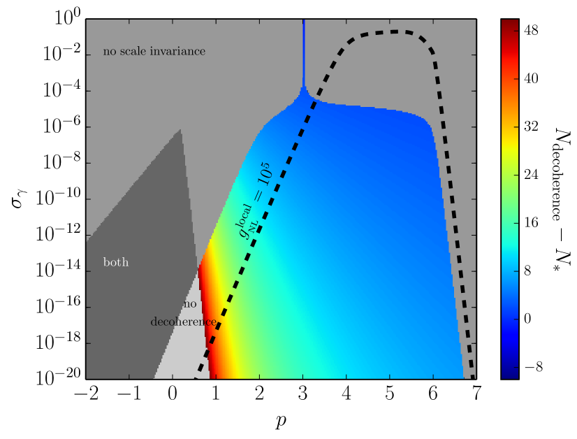
Figure 4: Same as Fig. 3 but with $H\ell_{\mathrm{E}}=10^{-6}$.

In this section, we use the above results to derive observational constraints on the interaction strength with the environment, hence on the amount of decoherence cosmological perturbations can have undergone in the early Universe. Concretely, this means constraints on the parameters $\sigma_{\gamma}$ and $p$. In LABEL:Martin:2018zbe, this was already done using the fact that the power spectrum is also modified by the interaction between the perturbations and the environment. In that reference, the constraints were summarized in figures similar to Figs. 3 and 4 in the present paper (Fig. 3 corresponds to Fig. 8 of LABEL:Martin:2018zbe where we have superimposed the constraint from non Gaussianity). In the space $(p,\sigma_{\gamma})$, the grey region labeled “no scale invariance” is a region that is excluded since the modifications caused by decoherence to the power spectrum spoil the quasi scale invariance to a level which is not observationally acceptable. The light grey region labeled “no decoherence” is a region where the corrections to the power spectrum are acceptable but where the strength of the interaction is so small that decoherence itself does not take place. The region “both” is a region where both actually happen: the interaction strength is too low to yield decoherence, but already too large to preserve the quasi scale invariance of the power spectrum. The coloured region is where decoherence occurs without modifying too much the power spectrum. The colour code, indicated by the colour bar on the right-hand side of the plot, indicates the number of $e$-folds at which decoherence takes place for the scale $k_{*}$, measured with respect to a reference time $N_{*}$ that corresponds to when the scale $k_{*}$ crosses out the Hubble radius during inflation.

A striking property of these figures is the vertical blue thin line centred at $p=3$. This corresponds to a situation where the corrections to the power spectrum originating from decoherence are themselves almost scale invariant [it is interesting to notice that for $p=3$ we also find $g_{{}_{\mathrm{NL}}}$ to be scale invariant, see Eq. (3.2) and Fig. 2]. In that case, clearly, no constraint on $\sigma_{\gamma}$ can be set from the power spectrum. Summarising the results of LABEL:Martin:2018zbe, it was shown that quasi scale invariance imposes $\sigma_{\gamma}\ll(H\ell_{\mathrm{E}})^{2-p}/N_{{}_{\mathrm{T}}}$ if $p<2$, where $N_{{}_{\mathrm{T}}}$ is the total number of $e$-folds during inflation; if $2<p<6$, one has $\sigma_{\gamma}\ll 1/N_{{}_{\mathrm{T}}}$, except if $p=3$ as just mentioned; and for $p>6$, one obtains $\sigma_{\gamma}\ll e^{(6-p)(N-N_{*})}/N_{{}_{\mathrm{T}}}$. Let us notice that the correction to the power spectrum and $g_{{}_{\mathrm{NL}}}$ have similar properties: for $p<2$, both depend on $H\ell_{\mathrm{E}}$, for $p>6$, both increase on super-Hubble scales, while for $4<p<6$ both are independent of $H\ell_{\mathrm{E}}$ and freeze on super-Hubble scales. The only difference is when $2<p<4$, where the corrections to the power spectrum are independent of $H\ell_{\mathrm{E}}$ and roughly independent of $p$, contrary to the trispectrum.

For this reason, the constraints from the trispectrum are qualitatively similar to the ones from the power spectrum, though quantitatively different. As already mentioned, CMB measurements indicate that the parameter $g_{{}_{\mathrm{NL}}}^{\mathrm{local}}$ is such that $g_{{}_{\mathrm{NL}}}^{\mathrm{local}}=(-9.0+7.7)\times 10^{4}$ at the one-sigma level [24]. Let us notice that this constraint only applies to a constant, scale-independent $g_{{}_{\mathrm{NL}}}^{\mathrm{local}}$, which not the case here since $g_{{}_{\mathrm{NL}}}^{\mathrm{local}}$ explicitly depends on $\alpha$ (except if $p>4$) and on $k$ (except if $p=3$, see Fig. 2). In principle, one should redo the Planck analysis and derive new constraints for the specific type of trispectrum originating from decoherence. Such an analysis is interesting but clearly beyond the scope of this paper. In addition, this would only improve the constraints discussed here which can thus be viewed as conservative.

Using the results of Sec. 3.2, in Figs. 3 and 4 we have superimposed the constraint coming from the non observation of a trispectrum in the CMB, see the black dashed line (the region above this line being excluded since it leads to $|g_{{}_{\mathrm{NL}}}|>10^{5}$). Fig. 3 corresponds to $H\ell_{\mathrm{E}}=10^{-3}$ while Fig. 4 is for $H\ell_{\mathrm{E}}=10^{-6}$. Technically, evaluating the expressions of $g_{{}_{\mathrm{NL}}}^{\mathrm{local}}$ derived in Sec. 3.2 at $k=k_{*}$, one finds

$$\sigma_{\gamma}<\begin{cases}\dfrac{81}{25}(4-p)2^{8-p}\pi^{4}\mathcal{P}_{\zeta}\left(k_{*}\right)\sigma\left(g_{{}_{\mathrm{NL}}}^{\mathrm{local}}\right)(H\ell_{\mathrm{E}})^{4-p}\simeq\mathcal{O}\left(10^{-2}\right)(H\ell_{\mathrm{E}})^{4-p}\quad\mathrm{if}\quad p<4\,,\vspace{0.4cm}\\ \dfrac{243}{25}\pi^{4}\mathcal{P}_{\zeta}\left(k_{*}\right)\sigma\left(g_{{}_{\mathrm{NL}}}^{\mathrm{local}}\right)\simeq 0.2\quad\mathrm{if}\quad 4<p<6\,,\vspace{0.4cm}\\ \dfrac{81}{50}\pi^{4}p(p-6)(p-3)\sigma\left(g_{{}_{\mathrm{NL}}}^{\mathrm{local}}\right)\mathcal{P}_{\zeta}\left(k_{*}\right)e^{(6-p)\left(N-N_{*}\right)}\simeq e^{(6-p)\left(N-N_{*}\right)}\quad\mathrm{if}\quad p>6\,,\end{cases}$$ (4.1)

where $\sigma\left(g_{{}_{\mathrm{NL}}}^{\mathrm{local}}\right)\sim 10^{5}$ denotes the one-sigma contraint on $|g_{{}_{\mathrm{NL}}}^{\mathrm{local}}|$. From these expressions and from Figs. 3 and 4, one sees that when $p<4$, the most stringent constraint comes from the trispectrum while when $p>4$, it still comes from the power spectrum. To our knowledge, this is a rare example in cosmology where the constraints coming from the trispectrum can be more efficient than those coming from the power spectrum.

An important conclusion is the fact that, for $p=3$ (which in LABEL:Martin:2018zbe was shown to correspond to the case where the environment is made of a heavy test scalar fied), the vertical blue line discussed before is now excluded, if $H\ell_{\mathrm{E}}$ is sufficiently small (for $H\ell_{\mathrm{E}}\simeq 10^{-3}$ there is still a small portion of the line that is viable). In LABEL:Martin:2018zbe, it was shown that along the blue line, the corrections to the power spectrum are quasi scale-invariant but can still substantially change the predictions of a given model of inflation, thus opening up the possibility to detect decoherence effects in the power spectrum. A non-trivial consequence of the current work is that, because of the constraints on the trispectrum, this cannot happen for sufficiently small $H\ell_{\mathrm{E}}$, since current bounds on non Gaussianities already exclude such a possibility.

5 Conclusions

Let us now recap our main findings. In this article, we have argued that cosmological perturbations should be treated as an open quantum system rather than a close system. In that case, decoherence can take place, which may be important when one tries to understand the quantum-to-classical transition of cosmological perturbations, or if one wonders whether genuine quantum correlations can be observed in cosmological perturbations that would unveil their quantum mechanical origin [27, 28].

The interaction of the system with an environment also induces modifications to observable quantities such as the power spectrum [23]. In this work we have shown that non Gaussianities also unavoidably appear. These non Gaussianities show up at the level of the four-point correlation function (trispectrum) while the bispectrum still vanishes. Using the Planck constraint on $g_{{}_{\mathrm{NL}}}^{\mathrm{local}}$, we have derived new constraints on the strength of the interaction between the cosmological perturbations and the environment. Remarkably, in some regimes, these constraints are more stringent than those inferred from the two-point correlation function.

Despite the generic character of these results, some important questions remain to be addressed. As mentioned before, the Planck constraints on non Gaussianities we have used were derived assuming a scale-invariant $g_{{}_{\mathrm{NL}}}^{\mathrm{local}}$ parameter, while the $g_{{}_{\mathrm{NL}}}^{\mathrm{local}}$ parameter caused by decoherence is generally scale dependent. Let us also recall that we have focused on the trispectrum in the equilateral configuration, since in that case it can be obtained from a differential equation of order five that we could solve analytically. For an arbitrary configuration, one has to solve a differential equation of order sixteen, which makes the analysis more complicated but still numerically achievable. Although our analysis leads to conservative bounds, it would be interesting to improve them by testing the actual trispectrum pattern found in this paper.

Another interesting question is the form of the interaction assumed between the perturbations and the environment. Here, we have considered the cases of linear (for which there are no non Gaussianities at leading order in the interaction strength) and quadratic (for which non Gaussianities show up only in the trispectrum) interactions. Clearly, it would be important to consider higher-order interactions (for which we expect non-Gaussianities in higher correlation functions, since an interaction of order $n$ gives rise to non-vanishing connected $m$-point correlation functions for all $m$ even and smaller than $2n$). This was done for the power spectrum in LABEL:Martin:2018zbe where a diagrammatic calculation of the source $S_{n}$ is available. Unfortunately, such a tool does not seem to be available for non Gaussianities which makes the problem much harder. We hope to come back to these issues in the future.

Appendix A Correlators for linear interactions

As already discussed at the beginning of Sec. 3, the case of a linear interaction is peculiar since it has been shown in LABEL:Martin:2018zbe that the density matrix of cosmological perturbations remains Gaussian. Therefore, there is no need to calculate the higher-order correlation functions since the result is entirely given by the Wick theorem. As a consistency check, it is nevertheless interesting to perform the calculation of the three- and four-point correlation functions using Eq. (2.3) in order to see explicitly how Gaussianity is preserved.

The equations for the two-point correlation functions were established in LABEL:Martin:2018zbe and read

$$\frac{\mathrm{d}}{\mathrm{d}\eta}\left\langle\hat{v}_{{\bm{k}}_{1}}\hat{v}_{{\bm{k}}_{2}}\right\rangle =\left\langle\hat{v}_{{\bm{k}}_{1}}\hat{p}_{{\bm{k}}_{2}}+\hat{p}_{{\bm{k}}_{1}}\hat{v}_{{\bm{k}}_{2}}\right\rangle,$$ (A.1)

$$\frac{\mathrm{d}}{\mathrm{d}\eta}\left\langle\hat{v}_{{\bm{k}}_{1}}\hat{p}_{{\bm{k}}_{2}}\right\rangle =\left\langle\hat{p}_{{\bm{k}}_{1}}\hat{p}_{{\bm{k}}_{2}}\right\rangle-\omega^{2}(k_{2})\left\langle\hat{v}_{{\bm{k}}_{1}}\hat{v}_{{\bm{k}}_{2}}\right\rangle,$$ (A.2)

$$\frac{\mathrm{d}}{\mathrm{d}\eta}\left\langle\hat{p}_{{\bm{k}}_{1}}\hat{v}_{{\bm{k}}_{2}}\right\rangle =\left\langle\hat{p}_{{\bm{k}}_{1}}\hat{p}_{{\bm{k}}_{2}}\right\rangle-\omega^{2}(k_{1})\left\langle\hat{v}_{{\bm{k}}_{1}}\hat{v}_{{\bm{k}}_{2}}\right\rangle,$$ (A.3)

$$\frac{\mathrm{d}}{\mathrm{d}\eta}\left\langle\hat{p}_{{\bm{k}}_{1}}\hat{p}_{{\bm{k}}_{2}}\right\rangle =-\omega^{2}(k_{2})\left\langle\hat{p}_{{\bm{k}}_{1}}\hat{v}_{{\bm{k}}_{2}}\right\rangle-\omega^{2}(k_{1})\left\langle\hat{v}_{{\bm{k}}_{1}}\hat{p}_{{\bm{k}}_{2}}\right\rangle+\gamma(2\pi)^{3/2}\tilde{C}_{R}({\bm{k}}_{1})\delta({\bm{k}}_{1}+{\bm{k}}_{2}).$$ (A.4)

The presence of the environment manifests itself by the term proportional to $\gamma$ only in the evolution equation for $\left\langle\hat{p}_{\bm{k}_{1}}\hat{p}_{{\bm{k}}_{2}}\right\rangle$. It is responsible for the appearance of a modified power spectrum.

The calculation of the three-point correlators proceeds in the same way and one obtains

$$\frac{\mathrm{d}}{\mathrm{d}\eta}\left\langle\hat{v}_{{\bm{k}}_{1}}\hat{v}_{{\bm{k}}_{2}}\hat{v}_{{\bm{k}}_{3}}\right\rangle =\left\langle\hat{v}_{{\bm{k}}_{1}}\hat{v}_{{\bm{k}}_{2}}\hat{p}_{{\bm{k}}_{3}}\right\rangle+\left\langle\hat{v}_{{\bm{k}}_{1}}\hat{p}_{{\bm{k}}_{2}}\hat{v}_{{\bm{k}}_{3}}\right\rangle+\left\langle\hat{p}_{{\bm{k}}_{1}}\hat{v}_{{\bm{k}}_{2}}\hat{v}_{{\bm{k}}_{3}}\right\rangle,$$ (A.5)

$$\frac{\mathrm{d}}{\mathrm{d}\eta}\left\langle\hat{v}_{{\bm{k}}_{1}}\hat{v}_{{\bm{k}}_{2}}\hat{p}_{{\bm{k}}_{3}}\right\rangle =\left\langle\hat{v}_{{\bm{k}}_{1}}\hat{p}_{{\bm{k}}_{2}}\hat{p}_{{\bm{k}}_{3}}\right\rangle+\left\langle\hat{p}_{{\bm{k}}_{1}}\hat{v}_{{\bm{k}}_{2}}\hat{p}_{{\bm{k}}_{3}}\right\rangle-\omega^{2}(k_{3})\left\langle\hat{v}_{{\bm{k}}_{1}}\hat{v}_{{\bm{k}}_{2}}\hat{v}_{{\bm{k}}_{3}}\right\rangle,$$ (A.6)

$$\frac{\mathrm{d}}{\mathrm{d}\eta}\left\langle\hat{v}_{{\bm{k}}_{1}}\hat{p}_{{\bm{k}}_{2}}\hat{v}_{{\bm{k}}_{3}}\right\rangle =\left\langle\hat{v}_{{\bm{k}}_{1}}\hat{p}_{{\bm{k}}_{2}}\hat{p}_{{\bm{k}}_{3}}\right\rangle+\left\langle\hat{p}_{{\bm{k}}_{1}}\hat{p}_{{\bm{k}}_{2}}\hat{v}_{{\bm{k}}_{3}}\right\rangle-\omega^{2}(k_{2})\left\langle\hat{v}_{{\bm{k}}_{1}}\hat{v}_{{\bm{k}}_{2}}\hat{v}_{{\bm{k}}_{3}}\right\rangle,$$ (A.7)

$$\frac{\mathrm{d}}{\mathrm{d}\eta}\left\langle\hat{p}_{{\bm{k}}_{1}}\hat{v}_{{\bm{k}}_{2}}\hat{v}_{{\bm{k}}_{3}}\right\rangle =\left\langle\hat{p}_{{\bm{k}}_{1}}\hat{v}_{{\bm{k}}_{2}}\hat{p}_{{\bm{k}}_{3}}\right\rangle+\left\langle\hat{p}_{{\bm{k}}_{1}}\hat{p}_{{\bm{k}}_{2}}\hat{v}_{{\bm{k}}_{3}}\right\rangle-\omega^{2}(k_{1})\left\langle\hat{v}_{{\bm{k}}_{1}}\hat{v}_{{\bm{k}}_{2}}\hat{v}_{{\bm{k}}_{3}}\right\rangle,$$ (A.8)

$$\frac{\mathrm{d}}{\mathrm{d}\eta}\left\langle\hat{v}_{{\bm{k}}_{1}}\hat{p}_{{\bm{k}}_{2}}\hat{p}_{{\bm{k}}_{3}}\right\rangle =\left\langle\hat{p}_{{\bm{k}}_{1}}\hat{p}_{{\bm{k}}_{2}}\hat{p}_{{\bm{k}}_{3}}\right\rangle-\omega^{2}(k_{3})\left\langle\hat{v}_{{\bm{k}}_{1}}\hat{p}_{{\bm{k}}_{2}}\hat{v}_{{\bm{k}}_{3}}\right\rangle-\omega^{2}(k_{2})\left\langle\hat{v}_{{\bm{k}}_{1}}\hat{v}_{{\bm{k}}_{2}}\hat{p}_{{\bm{k}}_{3}}\right\rangle,$$ (A.9)

$$\frac{\mathrm{d}}{\mathrm{d}\eta}\left\langle\hat{p}_{{\bm{k}}_{1}}\hat{v}_{{\bm{k}}_{2}}\hat{p}_{{\bm{k}}_{3}}\right\rangle =\left\langle\hat{p}_{{\bm{k}}_{1}}\hat{p}_{{\bm{k}}_{2}}\hat{p}_{{\bm{k}}_{3}}\right\rangle-\omega^{2}(k_{1})\left\langle\hat{v}_{{\bm{k}}_{1}}\hat{v}_{{\bm{k}}_{2}}\hat{p}_{{\bm{k}}_{3}}\right\rangle-\omega^{2}(k_{3})\left\langle\hat{p}_{{\bm{k}}_{1}}\hat{v}_{{\bm{k}}_{2}}\hat{v}_{{\bm{k}}_{3}}\right\rangle,$$ (A.10)

$$\frac{\mathrm{d}}{\mathrm{d}\eta}\left\langle\hat{p}_{{\bm{k}}_{1}}\hat{p}_{{\bm{k}}_{2}}\hat{v}_{{\bm{k}}_{3}}\right\rangle =\left\langle\hat{p}_{{\bm{k}}_{1}}\hat{p}_{{\bm{k}}_{2}}\hat{p}_{{\bm{k}}_{3}}\right\rangle-\omega^{2}(k_{2})\left\langle\hat{p}_{{\bm{k}}_{1}}\hat{v}_{{\bm{k}}_{2}}\hat{v}_{{\bm{k}}_{3}}\right\rangle-\omega^{2}(k_{1})\left\langle\hat{v}_{{\bm{k}}_{1}}\hat{p}_{{\bm{k}}_{2}}\hat{v}_{{\bm{k}}_{3}}\right\rangle,$$ (A.11)

$$\frac{\mathrm{d}}{\mathrm{d}\eta}\left\langle\hat{p}_{{\bm{k}}_{1}}\hat{p}_{{\bm{k}}_{2}}\hat{v}_{{\bm{k}}_{3}}\right\rangle =-\omega^{2}(k_{1})\left\langle\hat{v}_{{\bm{k}}_{1}}\hat{p}_{{\bm{k}}_{2}}\hat{p}_{{\bm{k}}_{3}}\right\rangle-\omega^{2}(k_{2})\left\langle\hat{p}_{{\bm{k}}_{1}}\hat{v}_{{\bm{k}}_{2}}\hat{p}_{{\bm{k}}_{3}}\right\rangle-\omega^{2}(k_{3})\left\langle\hat{p}_{{\bm{k}}_{1}}\hat{p}_{{\bm{k}}_{2}}\hat{v}_{{\bm{k}}_{3}}\right\rangle.$$ (A.12)

We notice that no term proportional to $\gamma$ is present in the above equations and this clearly implies that the three-point correlation functions all vanish if they are initially set to zero, in accordance with the fact that the system remains Gaussian if it is initially placed in the (Gaussian) Bunch-Davies vacuum state.

Let us now derive the evolution equations of the four-point correlators. Lengthy but straightforward calculations lead to

$$\frac{\mathrm{d}}{\mathrm{d}\eta}\left\langle\hat{v}_{{\bm{k}}_{1}}\hat{v}_{{\bm{k}}_{2}}\hat{v}_{{\bm{k}}_{3}}\hat{v}_{{\bm{k}}_{4}}\right\rangle =\left\langle\hat{v}_{{\bm{k}}_{1}}\hat{v}_{{\bm{k}}_{2}}\hat{v}_{{\bm{k}}_{3}}\hat{p}_{{\bm{k}}_{4}}\right\rangle+\left\langle\hat{v}_{{\bm{k}}_{1}}\hat{v}_{{\bm{k}}_{2}}\hat{p}_{{\bm{k}}_{3}}\hat{v}_{{\bm{k}}_{4}}\right\rangle+\left\langle\hat{v}_{{\bm{k}}_{1}}\hat{p}_{{\bm{k}}_{2}}\hat{v}_{{\bm{k}}_{3}}\hat{v}_{{\bm{k}}_{4}}\right\rangle+\left\langle\hat{p}_{{\bm{k}}_{1}}\hat{v}_{{\bm{k}}_{2}}\hat{v}_{{\bm{k}}_{3}}\hat{v}_{{\bm{k}}_{4}}\right\rangle,$$ (A.13)

$$\frac{\mathrm{d}}{\mathrm{d}\eta}\left\langle\hat{v}_{{\bm{k}}_{1}}\hat{v}_{{\bm{k}}_{2}}\hat{v}_{{\bm{k}}_{3}}\hat{p}_{{\bm{k}}_{4}}\right\rangle =\left\langle\hat{v}_{{\bm{k}}_{1}}\hat{v}_{{\bm{k}}_{2}}\hat{p}_{{\bm{k}}_{3}}\hat{p}_{{\bm{k}}_{4}}\right\rangle+\left\langle\hat{v}_{{\bm{k}}_{1}}\hat{p}_{{\bm{k}}_{2}}\hat{v}_{{\bm{k}}_{3}}\hat{p}_{{\bm{k}}_{4}}\right\rangle+\left\langle\hat{p}_{{\bm{k}}_{1}}\hat{v}_{{\bm{k}}_{2}}\hat{v}_{{\bm{k}}_{3}}\hat{p}_{{\bm{k}}_{4}}\right\rangle$$

$$-\omega^{2}(k_{4})\left\langle\hat{v}_{{\bm{k}}_{1}}\hat{v}_{{\bm{k}}_{2}}\hat{v}_{{\bm{k}}_{3}}\hat{v}_{{\bm{k}}_{4}}\right\rangle,$$ (A.14)

$$\frac{\mathrm{d}}{\mathrm{d}\eta}\left\langle\hat{v}_{{\bm{k}}_{1}}\hat{v}_{{\bm{k}}_{2}}\hat{p}_{{\bm{k}}_{3}}\hat{v}_{{\bm{k}}_{4}}\right\rangle =\left\langle\hat{p}_{{\bm{k}}_{1}}\hat{v}_{{\bm{k}}_{2}}\hat{p}_{{\bm{k}}_{3}}\hat{v}_{{\bm{k}}_{4}}\right\rangle+\left\langle\hat{v}_{{\bm{k}}_{1}}\hat{v}_{{\bm{k}}_{2}}\hat{p}_{{\bm{k}}_{3}}\hat{p}_{{\bm{k}}_{4}}\right\rangle+\left\langle\hat{v}_{{\bm{k}}_{1}}\hat{p}_{{\bm{k}}_{2}}\hat{p}_{{\bm{k}}_{3}}\hat{v}_{{\bm{k}}_{4}}\right\rangle$$

$$-\omega^{2}(k_{3})\left\langle\hat{v}_{{\bm{k}}_{1}}\hat{v}_{{\bm{k}}_{2}}\hat{v}_{{\bm{k}}_{3}}\hat{v}_{{\bm{k}}_{4}}\right\rangle,$$ (A.15)

$$\frac{\mathrm{d}}{\mathrm{d}\eta}\left\langle\hat{v}_{{\bm{k}}_{1}}\hat{p}_{{\bm{k}}_{2}}\hat{v}_{{\bm{k}}_{3}}\hat{v}_{{\bm{k}}_{4}}\right\rangle =\left\langle\hat{v}_{{\bm{k}}_{1}}\hat{p}_{{\bm{k}}_{2}}\hat{v}_{{\bm{k}}_{3}}\hat{p}_{{\bm{k}}_{4}}\right\rangle+\left\langle\hat{v}_{{\bm{k}}_{1}}\hat{p}_{{\bm{k}}_{2}}\hat{p}_{{\bm{k}}_{3}}\hat{v}_{{\bm{k}}_{4}}\right\rangle+\left\langle\hat{p}_{{\bm{k}}_{1}}\hat{p}_{{\bm{k}}_{2}}\hat{v}_{{\bm{k}}_{3}}\hat{v}_{{\bm{k}}_{4}}\right\rangle$$

$$-\omega^{2}(k_{2})\left\langle\hat{v}_{{\bm{k}}_{1}}\hat{v}_{{\bm{k}}_{2}}\hat{v}_{{\bm{k}}_{3}}\hat{v}_{{\bm{k}}_{4}}\right\rangle,$$ (A.16)

$$\frac{\mathrm{d}}{\mathrm{d}\eta}\left\langle\hat{p}_{{\bm{k}}_{1}}\hat{v}_{{\bm{k}}_{2}}\hat{v}_{{\bm{k}}_{3}}\hat{v}_{{\bm{k}}_{4}}\right\rangle =\left\langle\hat{p}_{{\bm{k}}_{1}}\hat{v}_{{\bm{k}}_{2}}\hat{v}_{{\bm{k}}_{3}}\hat{p}_{{\bm{k}}_{4}}\right\rangle+\left\langle\hat{p}_{{\bm{k}}_{1}}\hat{v}_{{\bm{k}}_{2}}\hat{p}_{{\bm{k}}_{3}}\hat{v}_{{\bm{k}}_{4}}\right\rangle+\left\langle\hat{p}_{{\bm{k}}_{1}}\hat{p}_{{\bm{k}}_{2}}\hat{v}_{{\bm{k}}_{3}}\hat{v}_{{\bm{k}}_{4}}\right\rangle$$

$$-\omega^{2}(k_{1})\left\langle\hat{v}_{{\bm{k}}_{1}}\hat{v}_{{\bm{k}}_{2}}\hat{v}_{{\bm{k}}_{3}}\hat{v}_{{\bm{k}}_{4}}\right\rangle,$$ (A.17)

$$\frac{\mathrm{d}}{\mathrm{d}\eta}\left\langle\hat{v}_{{\bm{k}}_{1}}\hat{v}_{{\bm{k}}_{2}}\hat{p}_{{\bm{k}}_{3}}\hat{p}_{{\bm{k}}_{4}}\right\rangle =\left\langle\hat{v}_{{\bm{k}}_{1}}\hat{p}_{{\bm{k}}_{2}}\hat{p}_{{\bm{k}}_{3}}\hat{p}_{{\bm{k}}_{4}}\right\rangle+\left\langle\hat{p}_{{\bm{k}}_{1}}\hat{v}_{{\bm{k}}_{2}}\hat{p}_{{\bm{k}}_{3}}\hat{p}_{{\bm{k}}_{4}}\right\rangle-\omega^{2}(k_{4})\left\langle\hat{v}_{{\bm{k}}_{1}}\hat{v}_{{\bm{k}}_{2}}\hat{p}_{{\bm{k}}_{3}}\hat{v}_{{\bm{k}}_{4}}\right\rangle$$

$$-\omega^{2}(k_{3})\left\langle\hat{v}_{{\bm{k}}_{1}}\hat{v}_{{\bm{k}}_{2}}\hat{v}_{{\bm{k}}_{3}}\hat{p}_{{\bm{k}}_{4}}\right\rangle+\gamma(2\pi)^{3/2}\tilde{C}_{R}(k_{3})\left\langle\hat{v}_{{\bm{k}}_{1}}\hat{v}_{{\bm{k}}_{2}}\right\rangle\delta\left({\bm{k}}_{3}+{\bm{k}}_{4}\right),$$ (A.18)

$$\frac{\mathrm{d}}{\mathrm{d}\eta}\left\langle\hat{v}_{{\bm{k}}_{1}}\hat{p}_{{\bm{k}}_{2}}\hat{v}_{{\bm{k}}_{3}}\hat{p}_{{\bm{k}}_{4}}\right\rangle =\left\langle\hat{v}_{{\bm{k}}_{1}}\hat{p}_{{\bm{k}}_{2}}\hat{p}_{{\bm{k}}_{3}}\hat{p}_{{\bm{k}}_{4}}\right\rangle+\left\langle\hat{p}_{{\bm{k}}_{1}}\hat{p}_{{\bm{k}}_{2}}\hat{v}_{{\bm{k}}_{3}}\hat{p}_{{\bm{k}}_{4}}\right\rangle-\omega^{2}(k_{4})\left\langle\hat{v}_{{\bm{k}}_{1}}\hat{p}_{{\bm{k}}_{2}}\hat{v}_{{\bm{k}}_{3}}\hat{v}_{{\bm{k}}_{4}}\right\rangle$$

$$-\omega^{2}(k_{2})\left\langle\hat{v}_{{\bm{k}}_{1}}\hat{v}_{{\bm{k}}_{2}}\hat{v}_{{\bm{k}}_{3}}\hat{p}_{{\bm{k}}_{4}}\right\rangle+\gamma(2\pi)^{3/2}\tilde{C}_{R}(k_{2})\left\langle\hat{v}_{{\bm{k}}_{1}}\hat{v}_{{\bm{k}}_{3}}\right\rangle\delta\left({\bm{k}}_{2}+{\bm{k}}_{4}\right),$$ (A.19)

$$\frac{\mathrm{d}}{\mathrm{d}\eta}\left\langle\hat{p}_{{\bm{k}}_{1}}\hat{v}_{{\bm{k}}_{2}}\hat{v}_{{\bm{k}}_{3}}\hat{p}_{{\bm{k}}_{4}}\right\rangle =\left\langle\hat{p}_{{\bm{k}}_{1}}\hat{v}_{{\bm{k}}_{2}}\hat{p}_{{\bm{k}}_{3}}\hat{p}_{{\bm{k}}_{4}}\right\rangle+\left\langle\hat{p}_{{\bm{k}}_{1}}\hat{p}_{{\bm{k}}_{2}}\hat{v}_{{\bm{k}}_{3}}\hat{p}_{{\bm{k}}_{4}}\right\rangle-\omega^{2}(k_{4})\left\langle\hat{p}_{{\bm{k}}_{1}}\hat{v}_{{\bm{k}}_{2}}\hat{v}_{{\bm{k}}_{3}}\hat{v}_{{\bm{k}}_{4}}\right\rangle$$

$$-\omega^{2}(k_{1})\left\langle\hat{v}_{{\bm{k}}_{1}}\hat{v}_{{\bm{k}}_{2}}\hat{v}_{{\bm{k}}_{3}}\hat{p}_{{\bm{k}}_{4}}\right\rangle+\gamma(2\pi)^{3/2}\tilde{C}_{R}(k_{1})\left\langle\hat{v}_{{\bm{k}}_{2}}\hat{v}_{{\bm{k}}_{3}}\right\rangle\delta\left({\bm{k}}_{1}+{\bm{k}}_{4}\right),$$ (A.20)

$$\frac{\mathrm{d}}{\mathrm{d}\eta}\left\langle\hat{v}_{{\bm{k}}_{1}}\hat{p}_{{\bm{k}}_{2}}\hat{p}_{{\bm{k}}_{3}}\hat{v}_{{\bm{k}}_{4}}\right\rangle =\left\langle\hat{v}_{{\bm{k}}_{1}}\hat{p}_{{\bm{k}}_{2}}\hat{p}_{{\bm{k}}_{3}}\hat{p}_{{\bm{k}}_{4}}\right\rangle+\left\langle\hat{p}_{{\bm{k}}_{1}}\hat{p}_{{\bm{k}}_{2}}\hat{p}_{{\bm{k}}_{3}}\hat{v}_{{\bm{k}}_{4}}\right\rangle-\omega^{2}(k_{3})\left\langle\hat{v}_{{\bm{k}}_{1}}\hat{p}_{{\bm{k}}_{2}}\hat{v}_{{\bm{k}}_{3}}\hat{v}_{{\bm{k}}_{4}}\right\rangle$$

$$-\omega^{2}(k_{2})\left\langle\hat{v}_{{\bm{k}}_{1}}\hat{v}_{{\bm{k}}_{2}}\hat{p}_{{\bm{k}}_{3}}\hat{v}_{{\bm{k}}_{4}}\right\rangle+\gamma(2\pi)^{3/2}\tilde{C}_{R}(k_{2})\left\langle\hat{v}_{{\bm{k}}_{1}}\hat{v}_{{\bm{k}}_{4}}\right\rangle\delta\left({\bm{k}}_{2}+{\bm{k}}_{3}\right),$$ (A.21)

$$\frac{\mathrm{d}}{\mathrm{d}\eta}\left\langle\hat{p}_{{\bm{k}}_{1}}\hat{v}_{{\bm{k}}_{2}}\hat{p}_{{\bm{k}}_{3}}\hat{v}_{{\bm{k}}_{4}}\right\rangle =\left\langle\hat{p}_{{\bm{k}}_{1}}\hat{v}_{{\bm{k}}_{2}}\hat{p}_{{\bm{k}}_{3}}\hat{p}_{{\bm{k}}_{4}}\right\rangle+\left\langle\hat{p}_{{\bm{k}}_{1}}\hat{p}_{{\bm{k}}_{2}}\hat{p}_{{\bm{k}}_{3}}\hat{v}_{{\bm{k}}_{4}}\right\rangle-\omega^{2}(k_{3})\left\langle\hat{p}_{{\bm{k}}_{1}}\hat{v}_{{\bm{k}}_{2}}\hat{v}_{{\bm{k}}_{3}}\hat{v}_{{\bm{k}}_{4}}\right\rangle$$

$$-\omega^{2}(k_{1})\left\langle\hat{v}_{{\bm{k}}_{1}}\hat{v}_{{\bm{k}}_{2}}\hat{p}_{{\bm{k}}_{3}}\hat{v}_{{\bm{k}}_{4}}\right\rangle+\gamma(2\pi)^{3/2}\tilde{C}_{R}(k_{1})\left\langle\hat{v}_{{\bm{k}}_{2}}\hat{v}_{{\bm{k}}_{4}}\right\rangle\delta\left({\bm{k}}_{1}+{\bm{k}}_{3}\right),$$ (A.22)

$$\frac{\mathrm{d}}{\mathrm{d}\eta}\left\langle\hat{p}_{{\bm{k}}_{1}}\hat{p}_{{\bm{k}}_{2}}\hat{v}_{{\bm{k}}_{3}}\hat{v}_{{\bm{k}}_{4}}\right\rangle =\left\langle\hat{p}_{{\bm{k}}_{1}}\hat{p}_{{\bm{k}}_{2}}\hat{v}_{{\bm{k}}_{3}}\hat{p}_{{\bm{k}}_{4}}\right\rangle+\left\langle\hat{p}_{{\bm{k}}_{1}}\hat{p}_{{\bm{k}}_{2}}\hat{p}_{{\bm{k}}_{3}}\hat{v}_{{\bm{k}}_{4}}\right\rangle-\omega^{2}(k_{2})\left\langle\hat{p}_{{\bm{k}}_{1}}\hat{v}_{{\bm{k}}_{2}}\hat{v}_{{\bm{k}}_{3}}\hat{v}_{{\bm{k}}_{4}}\right\rangle$$

$$-\omega^{2}(k_{1})\left\langle\hat{v}_{{\bm{k}}_{1}}\hat{p}_{{\bm{k}}_{2}}\hat{v}_{{\bm{k}}_{3}}\hat{v}_{{\bm{k}}_{4}}\right\rangle+\gamma(2\pi)^{3/2}\tilde{C}_{R}(k_{1})\left\langle\hat{v}_{{\bm{k}}_{3}}\hat{v}_{{\bm{k}}_{4}}\right\rangle\delta\left({\bm{k}}_{1}+{\bm{k}}_{2}\right),$$ (A.23)

$$\frac{\mathrm{d}}{\mathrm{d}\eta}\left\langle\hat{v}_{{\bm{k}}_{1}}\hat{p}_{{\bm{k}}_{2}}\hat{p}_{{\bm{k}}_{3}}\hat{p}_{{\bm{k}}_{4}}\right\rangle =\left\langle\hat{p}_{{\bm{k}}_{1}}\hat{p}_{{\bm{k}}_{2}}\hat{p}_{{\bm{k}}_{3}}\hat{p}_{{\bm{k}}_{4}}\right\rangle-\omega^{2}(k_{4})\left\langle\hat{v}_{{\bm{k}}_{1}}\hat{p}_{{\bm{k}}_{2}}\hat{p}_{{\bm{k}}_{3}}\hat{v}_{{\bm{k}}_{4}}\right\rangle-\omega^{2}(k_{3})\left\langle\hat{v}_{{\bm{k}}_{1}}\hat{p}_{{\bm{k}}_{2}}\hat{v}_{{\bm{k}}_{3}}\hat{p}_{{\bm{k}}_{4}}\right\rangle$$

$$-\omega^{2}(k_{2})\left\langle\hat{v}_{{\bm{k}}_{1}}\hat{v}_{{\bm{k}}_{2}}\hat{p}_{{\bm{k}}_{3}}\hat{p}_{{\bm{k}}_{4}}\right\rangle+\gamma(2\pi)^{3/2}\tilde{C}_{R}(k_{3})\left\langle\hat{v}_{{\bm{k}}_{1}}\hat{p}_{{\bm{k}}_{2}}\right\rangle\delta\left({\bm{k}}_{3}+{\bm{k}}_{4}\right)$$

$$+\gamma(2\pi)^{3/2}\tilde{C}_{R}(k_{2})\left\langle\hat{v}_{{\bm{k}}_{1}}\hat{p}_{{\bm{k}}_{3}}\right\rangle\delta\left({\bm{k}}_{2}+{\bm{k}}_{4}\right)$$

$$+\gamma(2\pi)^{3/2}\tilde{C}_{R}(k_{2})\left\langle\hat{v}_{{\bm{k}}_{1}}\hat{p}_{{\bm{k}}_{4}}\right\rangle\delta\left({\bm{k}}_{2}+{\bm{k}}_{3}\right),$$ (A.24)

$$\frac{\mathrm{d}}{\mathrm{d}\eta}\left\langle\hat{p}_{{\bm{k}}_{1}}\hat{v}_{{\bm{k}}_{2}}\hat{p}_{{\bm{k}}_{3}}\hat{p}_{{\bm{k}}_{4}}\right\rangle =\left\langle\hat{p}_{{\bm{k}}_{1}}\hat{p}_{{\bm{k}}_{2}}\hat{p}_{{\bm{k}}_{3}}\hat{p}_{{\bm{k}}_{4}}\right\rangle-\omega^{2}(k_{4})\left\langle\hat{p}_{{\bm{k}}_{1}}\hat{v}_{{\bm{k}}_{2}}\hat{p}_{{\bm{k}}_{3}}\hat{v}_{{\bm{k}}_{4}}\right\rangle-\omega^{2}(k_{3})\left\langle\hat{p}_{{\bm{k}}_{1}}\hat{v}_{{\bm{k}}_{2}}\hat{v}_{{\bm{k}}_{3}}\hat{p}_{{\bm{k}}_{4}}\right\rangle$$

$$-\omega^{2}(k_{1})\left\langle\hat{v}_{{\bm{k}}_{1}}\hat{v}_{{\bm{k}}_{2}}\hat{p}_{{\bm{k}}_{3}}\hat{p}_{{\bm{k}}_{4}}\right\rangle+\gamma(2\pi)^{3/2}\tilde{C}_{R}(k_{3})\left\langle\hat{p}_{{\bm{k}}_{1}}\hat{v}_{{\bm{k}}_{2}}\right\rangle\delta\left({\bm{k}}_{3}+{\bm{k}}_{4}\right)$$

$$+\gamma(2\pi)^{3/2}\tilde{C}_{R}(k_{1})\left\langle\hat{v}_{{\bm{k}}_{2}}\hat{p}_{{\bm{k}}_{3}}\right\rangle\delta\left({\bm{k}}_{1}+{\bm{k}}_{4}\right)$$

$$+\gamma(2\pi)^{3/2}\tilde{C}_{R}(k_{1})\left\langle\hat{v}_{{\bm{k}}_{2}}\hat{p}_{{\bm{k}}_{4}}\right\rangle\delta\left({\bm{k}}_{1}+{\bm{k}}_{3}\right),$$ (A.25)

$$\frac{\mathrm{d}}{\mathrm{d}\eta}\left\langle\hat{p}_{{\bm{k}}_{1}}\hat{p}_{{\bm{k}}_{2}}\hat{v}_{{\bm{k}}_{3}}\hat{p}_{{\bm{k}}_{4}}\right\rangle =\left\langle\hat{p}_{{\bm{k}}_{1}}\hat{p}_{{\bm{k}}_{2}}\hat{p}_{{\bm{k}}_{3}}\hat{p}_{{\bm{k}}_{4}}\right\rangle-\omega^{2}(k_{4})\left\langle\hat{p}_{{\bm{k}}_{1}}\hat{p}_{{\bm{k}}_{2}}\hat{v}_{{\bm{k}}_{3}}\hat{v}_{{\bm{k}}_{4}}\right\rangle-\omega^{2}(k_{2})\left\langle\hat{p}_{{\bm{k}}_{1}}\hat{v}_{{\bm{k}}_{2}}\hat{v}_{{\bm{k}}_{3}}\hat{p}_{{\bm{k}}_{4}}\right\rangle$$

$$-\omega^{2}(k_{1})\left\langle\hat{v}_{{\bm{k}}_{1}}\hat{p}_{{\bm{k}}_{2}}\hat{v}_{{\bm{k}}_{3}}\hat{p}_{{\bm{k}}_{4}}\right\rangle+\gamma(2\pi)^{3/2}\tilde{C}_{R}(k_{2})\left\langle\hat{p}_{{\bm{k}}_{1}}\hat{v}_{{\bm{k}}_{3}}\right\rangle\delta\left({\bm{k}}_{2}+{\bm{k}}_{4}\right)$$

$$+\gamma(2\pi)^{3/2}\tilde{C}_{R}(k_{1})\left\langle\hat{p}_{{\bm{k}}_{2}}\hat{v}_{{\bm{k}}_{3}}\right\rangle\delta\left({\bm{k}}_{1}+{\bm{k}}_{4}\right)$$

$$+\gamma(2\pi)^{3/2}\tilde{C}_{R}(k_{1})\left\langle\hat{v}_{{\bm{k}}_{3}}\hat{p}_{{\bm{k}}_{4}}\right\rangle\delta\left({\bm{k}}_{1}+{\bm{k}}_{2}\right),$$ (A.26)

$$\frac{\mathrm{d}}{\mathrm{d}\eta}\left\langle\hat{p}_{{\bm{k}}_{1}}\hat{p}_{{\bm{k}}_{2}}\hat{p}_{{\bm{k}}_{3}}\hat{v}_{{\bm{k}}_{4}}\right\rangle =\left\langle\hat{p}_{{\bm{k}}_{1}}\hat{p}_{{\bm{k}}_{2}}\hat{p}_{{\bm{k}}_{3}}\hat{p}_{{\bm{k}}_{4}}\right\rangle-\omega^{2}(k_{3})\left\langle\hat{p}_{{\bm{k}}_{1}}\hat{p}_{{\bm{k}}_{2}}\hat{v}_{{\bm{k}}_{3}}\hat{v}_{{\bm{k}}_{4}}\right\rangle-\omega^{2}(k_{2})\left\langle\hat{p}_{{\bm{k}}_{1}}\hat{v}_{{\bm{k}}_{2}}\hat{p}_{{\bm{k}}_{3}}\hat{v}_{{\bm{k}}_{4}}\right\rangle$$

$$-\omega^{2}(k_{1})\left\langle\hat{v}_{{\bm{k}}_{1}}\hat{p}_{{\bm{k}}_{2}}\hat{p}_{{\bm{k}}_{3}}\hat{v}_{{\bm{k}}_{4}}\right\rangle+\gamma(2\pi)^{3/2}\tilde{C}_{R}(k_{1})\left\langle\hat{p}_{{\bm{k}}_{1}}\hat{v}_{{\bm{k}}_{4}}\right\rangle\delta\left({\bm{k}}_{2}+{\bm{k}}_{3}\right)$$

$$+\gamma(2\pi)^{3/2}\tilde{C}_{R}(k_{1})\left\langle\hat{p}_{{\bm{k}}_{2}}\hat{v}_{{\bm{k}}_{4}}\right\rangle\delta\left({\bm{k}}_{1}+{\bm{k}}_{3}\right)$$

$$+\gamma(2\pi)^{3/2}\tilde{C}_{R}(k_{1})\left\langle\hat{p}_{{\bm{k}}_{3}}\hat{v}_{{\bm{k}}_{4}}\right\rangle\delta\left({\bm{k}}_{1}+{\bm{k}}_{2}\right),$$ (A.27)

$$\frac{\mathrm{d}}{\mathrm{d}\eta}\left\langle\hat{p}_{{\bm{k}}_{1}}\hat{p}_{{\bm{k}}_{2}}\hat{p}_{{\bm{k}}_{3}}\hat{p}_{{\bm{k}}_{4}}\right\rangle =-\omega^{2}(k_{4})\left\langle\hat{p}_{{\bm{k}}_{1}}\hat{p}_{{\bm{k}}_{2}}\hat{p}_{{\bm{k}}_{3}}\hat{v}_{{\bm{k}}_{4}}\right\rangle-\omega^{2}(k_{3})\left\langle\hat{p}_{{\bm{k}}_{1}}\hat{p}_{{\bm{k}}_{2}}\hat{v}_{{\bm{k}}_{3}}\hat{p}_{{\bm{k}}_{4}}\right\rangle$$

$$-\omega^{2}(k_{2})\left\langle\hat{p}_{{\bm{k}}_{1}}\hat{v}_{{\bm{k}}_{2}}\hat{p}_{{\bm{k}}_{3}}\hat{p}_{{\bm{k}}_{4}}\right\rangle-\omega^{2}(k_{1})\left\langle\hat{v}_{{\bm{k}}_{1}}\hat{p}_{{\bm{k}}_{2}}\hat{p}_{{\bm{k}}_{3}}\hat{p}_{{\bm{k}}_{4}}\right\rangle$$

$$+\gamma(2\pi)^{3/2}\tilde{C}_{R}(k_{3})\left\langle\hat{p}_{{\bm{k}}_{1}}\hat{p}_{{\bm{k}}_{2}}\right\rangle\delta\left({\bm{k}}_{3}+{\bm{k}}_{4}\right)$$

$$+\gamma(2\pi)^{3/2}\tilde{C}_{R}(k_{2})\left\langle\hat{p}_{{\bm{k}}_{1}}\hat{p}_{{\bm{k}}_{3}}\right\rangle\delta\left({\bm{k}}_{2}+{\bm{k}}_{4}\right)$$

$$+\gamma(2\pi)^{3/2}\tilde{C}_{R}(k_{1})\left\langle\hat{p}_{{\bm{k}}_{2}}\hat{p}_{{\bm{k}}_{3}}\right\rangle\delta\left({\bm{k}}_{1}+{\bm{k}}_{4}\right)$$

$$+\gamma(2\pi)^{3/2}\tilde{C}_{R}(k_{2})\left\langle\hat{p}_{{\bm{k}}_{1}}\hat{p}_{{\bm{k}}_{4}}\right\rangle\delta\left({\bm{k}}_{2}+{\bm{k}}_{4}\right)$$

$$+\gamma(2\pi)^{3/2}\tilde{C}_{R}(k_{1})\left\langle\hat{p}_{{\bm{k}}_{2}}\hat{p}_{{\bm{k}}_{4}}\right\rangle\delta\left({\bm{k}}_{1}+{\bm{k}}_{3}\right)$$

$$+\gamma(2\pi)^{3/2}\tilde{C}_{R}(k_{1})\left\langle\hat{p}_{{\bm{k}}_{3}}\hat{p}_{{\bm{k}}_{4}}\right\rangle\delta\left({\bm{k}}_{1}+{\bm{k}}_{2}\right).$$ (A.28)

We notice that, contrary to the three-point correlators, the above equations contain terms proportional to $\gamma$. This is because these correlators contain disconnected diagrams, i.e. products of power spectra which we have shown are affected by the environment, see Eq. (A.4). Non Gaussianities are however not present in the connected four-point correlators that one obtains from subtracting the contribution of Wick theorem (for instance, $\left\langle\hat{v}_{{\bm{k}}_{1}}\hat{p}_{{\bm{k}}_{2}}\hat{p}_{{\bm{k}}_{3}}\hat{v}_{{\bm{k}}_{4}}\right\rangle_{\mathrm{c}}=\left\langle\hat{v}_{{\bm{k}}_{1}}\hat{p}_{{\bm{k}}_{2}}\hat{p}_{{\bm{k}}_{3}}\hat{v}_{{\bm{k}}_{4}}\right\rangle-\left\langle\hat{v}_{{\bm{k}}_{1}}\hat{p}_{{\bm{k}}_{2}}\right\rangle\left\langle\hat{p}_{{\bm{k}}_{3}}\hat{v}_{{\bm{k}}_{4}}\right\rangle-\left\langle\hat{v}_{{\bm{k}}_{1}}\hat{p}_{{\bm{k}}_{3}}\right\rangle\left\langle\hat{p}_{{\bm{k}}_{2}}\hat{v}_{{\bm{k}}_{4}}\right\rangle-\left\langle\hat{v}_{{\bm{k}}_{1}}\hat{v}_{{\bm{k}}_{4}}\right\rangle\left\langle\hat{p}_{{\bm{k}}_{2}}\hat{p}_{{\bm{k}}_{3}}\right\rangle$, where the index $\mathrm{c}$ denotes the connected part of the correlator). The evolution equations for the connected four-point correlators can be derived from the previous set of equations making use of Eqs. (A.1)-(A.4), and one can check that the corresponding system of equations no longer contains terms proportional to $\gamma$ (one may have noticed that the terms proportional to $\gamma$ have the same form in the equations for the two-point and for the four-point correlators). This is again consistent with the fact that the density matrix of the system remains Gaussian.

Appendix B Correlators for quadratic interactions

In this section, we derive the equations for the three- and four-point correlation functions in the case where the interaction between the system and the environment is proportional to the square of the Mukhanov-Sasaki variable. Let us recall that the equations for the two-point correlators have been established in LABEL:Martin:2018zbe and are given by

$$\frac{\mathrm{d}}{\mathrm{d}\eta}\left\langle\hat{v}_{{\bm{k}}_{1}}\hat{v}_{{\bm{k}}_{2}}\right\rangle =\left\langle\hat{v}_{{\bm{k}}_{1}}\hat{p}_{{\bm{k}}_{2}}+\hat{p}_{{\bm{k}}_{1}}\hat{v}_{{\bm{k}}_{2}}\right\rangle,$$ (B.1)

$$\frac{\mathrm{d}}{\mathrm{d}\eta}\left\langle\hat{v}_{{\bm{k}}_{1}}\hat{p}_{{\bm{k}}_{2}}\right\rangle =\left\langle\hat{p}_{{\bm{k}}_{1}}\hat{p}_{{\bm{k}}_{2}}\right\rangle-\omega^{2}(k_{2})\left\langle\hat{v}_{{\bm{k}}_{1}}\hat{v}_{{\bm{k}}_{2}}\right\rangle,$$ (B.2)

$$\frac{\mathrm{d}}{\mathrm{d}\eta}\left\langle\hat{p}_{{\bm{k}}_{1}}\hat{v}_{{\bm{k}}_{2}}\right\rangle =\left\langle\hat{p}_{{\bm{k}}_{1}}\hat{p}_{{\bm{k}}_{2}}\right\rangle-\omega^{2}(k_{1})\left\langle\hat{v}_{{\bm{k}}_{1}}\hat{v}_{{\bm{k}}_{2}}\right\rangle,$$ (B.3)

$$\frac{\mathrm{d}}{\mathrm{d}\eta}\left\langle\hat{p}_{{\bm{k}}_{1}}\hat{p}_{{\bm{k}}_{2}}\right\rangle =-\omega^{2}(k_{2})\left\langle\hat{p}_{{\bm{k}}_{1}}\hat{v}_{{\bm{k}}_{2}}\right\rangle-\omega^{2}(k_{1})\left\langle\hat{v}_{{\bm{k}}_{1}}\hat{p}_{{\bm{k}}_{2}}\right\rangle$$ (B.4)

$$+\frac{4\gamma}{(2\pi)^{3/2}}\int\mathrm{d}^{3}{\bm{k}}\,\tilde{C}_{R}(\bm{k})\left\langle\hat{v}_{{\bm{k}}+{\bm{k}}_{1}}\hat{v}_{-{\bm{k}}+{\bm{k}}_{2}}\right\rangle.$$ (B.5)

B.1 Three-point correlators

Using the Lindblad equation (2.3), the equations controlling the evolution of the three-point correlators can be expressed as

$$\frac{\mathrm{d}}{\mathrm{d}\eta}\left\langle\hat{v}_{{\bm{k}}_{1}}\hat{v}_{{\bm{k}}_{2}}\hat{v}_{{\bm{k}}_{3}}\right\rangle =\left\langle\hat{v}_{{\bm{k}}_{1}}\hat{v}_{{\bm{k}}_{2}}\hat{p}_{{\bm{k}}_{3}}\right\rangle+\left\langle\hat{v}_{{\bm{k}}_{1}}\hat{p}_{{\bm{k}}_{2}}\hat{v}_{{\bm{k}}_{3}}\right\rangle+\left\langle\hat{p}_{{\bm{k}}_{1}}\hat{v}_{{\bm{k}}_{2}}\hat{v}_{{\bm{k}}_{3}}\right\rangle,$$ (B.6)

$$\frac{\mathrm{d}}{\mathrm{d}\eta}\left\langle\hat{v}_{{\bm{k}}_{1}}\hat{v}_{{\bm{k}}_{2}}\hat{p}_{{\bm{k}}_{3}}\right\rangle =\left\langle\hat{v}_{{\bm{k}}_{1}}\hat{p}_{{\bm{k}}_{2}}\hat{p}_{{\bm{k}}_{3}}\right\rangle+\left\langle\hat{p}_{{\bm{k}}_{1}}\hat{v}_{{\bm{k}}_{2}}\hat{p}_{{\bm{k}}_{3}}\right\rangle-\omega^{2}(k_{3})\left\langle\hat{v}_{{\bm{k}}_{1}}\hat{v}_{{\bm{k}}_{2}}\hat{v}_{{\bm{k}}_{3}}\right\rangle,$$ (B.7)

$$\frac{\mathrm{d}}{\mathrm{d}\eta}\left\langle\hat{v}_{{\bm{k}}_{1}}\hat{p}_{{\bm{k}}_{2}}\hat{v}_{{\bm{k}}_{3}}\right\rangle =\left\langle\hat{v}_{{\bm{k}}_{1}}\hat{p}_{{\bm{k}}_{2}}\hat{p}_{{\bm{k}}_{3}}\right\rangle+\left\langle\hat{p}_{{\bm{k}}_{1}}\hat{p}_{{\bm{k}}_{2}}\hat{v}_{{\bm{k}}_{3}}\right\rangle-\omega^{2}(k_{2})\left\langle\hat{v}_{{\bm{k}}_{1}}\hat{v}_{{\bm{k}}_{2}}\hat{v}_{{\bm{k}}_{3}}\right\rangle,$$ (B.8)

$$\frac{\mathrm{d}}{\mathrm{d}\eta}\left\langle\hat{p}_{{\bm{k}}_{1}}\hat{v}_{{\bm{k}}_{2}}\hat{v}_{{\bm{k}}_{3}}\right\rangle =\left\langle\hat{p}_{{\bm{k}}_{1}}\hat{v}_{{\bm{k}}_{2}}\hat{p}_{{\bm{k}}_{3}}\right\rangle+\left\langle\hat{p}_{{\bm{k}}_{1}}\hat{p}_{{\bm{k}}_{2}}\hat{v}_{{\bm{k}}_{3}}\right\rangle-\omega^{2}(k_{1})\left\langle\hat{v}_{{\bm{k}}_{1}}\hat{v}_{{\bm{k}}_{2}}\hat{v}_{{\bm{k}}_{3}}\right\rangle,$$ (B.9)

$$\frac{\mathrm{d}}{\mathrm{d}\eta}\left\langle\hat{v}_{{\bm{k}}_{1}}\hat{p}_{{\bm{k}}_{2}}\hat{p}_{{\bm{k}}_{3}}\right\rangle =\left\langle\hat{p}_{{\bm{k}}_{1}}\hat{p}_{{\bm{k}}_{2}}\hat{p}_{{\bm{k}}_{3}}\right\rangle-\omega^{2}(k_{3})\left\langle\hat{v}_{{\bm{k}}_{1}}\hat{p}_{{\bm{k}}_{2}}\hat{v}_{{\bm{k}}_{3}}\right\rangle-\omega^{2}(k_{2})\left\langle\hat{v}_{{\bm{k}}_{1}}\hat{v}_{{\bm{k}}_{2}}\hat{p}_{{\bm{k}}_{3}}\right\rangle$$

$$+\frac{4\gamma}{(2\pi)^{3/2}}\int{\mathrm{d}}^{3}{\bm{k}}\,\tilde{C}_{R}(k)\left\langle\hat{v}_{{\bm{k}}_{1}}\hat{v}_{{\bm{k}}_{2}-{\bm{k}}}\hat{v}_{{\bm{k}}+{\bm{k}}_{3}}\right\rangle,$$ (B.10)

$$\frac{\mathrm{d}}{\mathrm{d}\eta}\left\langle\hat{p}_{{\bm{k}}_{1}}\hat{v}_{{\bm{k}}_{2}}\hat{p}_{{\bm{k}}_{3}}\right\rangle =\left\langle\hat{p}_{{\bm{k}}_{1}}\hat{p}_{{\bm{k}}_{2}}\hat{p}_{{\bm{k}}_{3}}\right\rangle-\omega^{2}(k_{1})\left\langle\hat{v}_{{\bm{k}}_{1}}\hat{v}_{{\bm{k}}_{2}}\hat{p}_{{\bm{k}}_{3}}\right\rangle-\omega^{2}(k_{3})\left\langle\hat{p}_{{\bm{k}}_{1}}\hat{v}_{{\bm{k}}_{2}}\hat{v}_{{\bm{k}}_{3}}\right\rangle$$

$$+\frac{4\gamma}{(2\pi)^{3/2}}\int{\mathrm{d}}^{3}{\bm{k}}\,\tilde{C}_{R}(k)\left\langle\hat{v}_{{\bm{k}}_{1}-{\bm{k}}}\hat{v}_{{\bm{k}}_{2}}\hat{v}_{{\bm{k}}+{\bm{k}}_{3}}\right\rangle,$$ (B.11)

$$\frac{\mathrm{d}}{\mathrm{d}\eta}\left\langle\hat{p}_{{\bm{k}}_{1}}\hat{p}_{{\bm{k}}_{2}}\hat{v}_{{\bm{k}}_{3}}\right\rangle =\left\langle\hat{p}_{{\bm{k}}_{1}}\hat{p}_{{\bm{k}}_{2}}\hat{p}_{{\bm{k}}_{3}}\right\rangle-\omega^{2}(k_{2})\left\langle\hat{p}_{{\bm{k}}_{1}}\hat{v}_{{\bm{k}}_{2}}\hat{v}_{{\bm{k}}_{3}}\right\rangle-\omega^{2}(k_{1})\left\langle\hat{v}_{{\bm{k}}_{1}}\hat{p}_{{\bm{k}}_{2}}\hat{v}_{{\bm{k}}_{3}}\right\rangle$$

$$+\frac{4\gamma}{(2\pi)^{3/2}}\int{\mathrm{d}}^{3}{\bm{k}}\,\tilde{C}_{R}(k)\left\langle\hat{v}_{{\bm{k}}_{1}-{\bm{k}}}\hat{v}_{{\bm{k}}+{\bm{k}}_{2}}\hat{v}_{{\bm{k}}_{3}}\right\rangle,$$ (B.12)

$$\frac{\mathrm{d}}{\mathrm{d}\eta}\left\langle\hat{p}_{{\bm{k}}_{1}}\hat{p}_{{\bm{k}}_{2}}\hat{v}_{{\bm{k}}_{3}}\right\rangle =-\omega^{2}(k_{1})\left\langle\hat{v}_{{\bm{k}}_{1}}\hat{p}_{{\bm{k}}_{2}}\hat{p}_{{\bm{k}}_{3}}\right\rangle-\omega^{2}(k_{2})\left\langle\hat{p}_{{\bm{k}}_{1}}\hat{v}_{{\bm{k}}_{2}}\hat{p}_{{\bm{k}}_{3}}\right\rangle-\omega^{2}(k_{3})\left\langle\hat{p}_{{\bm{k}}_{1}}\hat{p}_{{\bm{k}}_{2}}\hat{v}_{{\bm{k}}_{3}}\right\rangle$$

$$+\frac{4\gamma}{(2\pi)^{3/2}}\int{\mathrm{d}}^{3}{\bm{k}}\,\tilde{C}_{R}(k)\bigl{(}\left\langle\hat{p}_{{\bm{k}}_{1}}\hat{v}_{{\bm{k}}_{2}-{\bm{k}}}\hat{v}_{{\bm{k}}+{\bm{k}}_{3}}\right\rangle+\left\langle\hat{v}_{{\bm{k}}_{1}-{\bm{k}}}\hat{p}_{{\bm{k}}_{2}}\hat{v}_{{\bm{k}}+{\bm{k}}_{3}}\right\rangle$$

$$+\left\langle\hat{v}_{{\bm{k}}_{1}+{\bm{k}}}\hat{v}_{{\bm{k}}_{2}-{\bm{k}}}\hat{p}_{{\bm{k}}_{3}}\right\rangle\bigr{)}.$$ (B.13)

We notice that the above system of equations contain terms proportional to $\gamma$. As is typical for quadratic interactions, see Eqs. (B.1)-(B.4), and contrary to the case of linear interactions, see Eqs. (A.1)-(A.4), they involve integrals over momentum. However, those terms are also all expressed in terms of three-point correlators [in the very same way, in the case of the equations (B.1)-(B.4) for the two-point correlation functions, the term proportional to $\gamma$ is proportional to the power spectrum]. Since these corrections must be evaluated in the free theory (we recall that the Lindblad equation is established perturbatively in the interaction strength and is valid at first order in $\gamma$ only), this implies that they all vanish at leading order in $\gamma$. As already mentioned in the main text, we conclude that the Lindblad equation does not lead to a non-vanishing bispectrum in that case.

B.2 Four-point correlators

This is why one needs to calculate the four-point correlators (namely the trispectrum) if one wants to exhibit non Gaussianities. As already discussed in Appendix A, the fact that these equations contain terms proportional to $\gamma$ does not necessarily imply that non Gaussianities are present. For this reason, we now directly proceed to the calculation of the connected part of the four-point correlators. Straightforward but lengthy calculations lead to the following expressions

$$\frac{\mathrm{d}}{\mathrm{d}\eta}\left\langle\hat{v}_{{\bm{k}}_{1}}\hat{v}_{{\bm{k}}_{2}}\hat{v}_{{\bm{k}}_{3}}\hat{v}_{{\bm{k}}_{4}}\right\rangle_{\mathrm{c}} =\left\langle\hat{v}_{{\bm{k}}_{1}}\hat{v}_{{\bm{k}}_{2}}\hat{v}_{{\bm{k}}_{3}}\hat{p}_{{\bm{k}}_{4}}\right\rangle_{\mathrm{c}}+\left\langle\hat{v}_{{\bm{k}}_{1}}\hat{v}_{{\bm{k}}_{2}}\hat{p}_{{\bm{k}}_{3}}\hat{v}_{{\bm{k}}_{4}}\right\rangle_{\mathrm{c}}+\left\langle\hat{v}_{{\bm{k}}_{1}}\hat{p}_{{\bm{k}}_{2}}\hat{v}_{{\bm{k}}_{3}}\hat{v}_{{\bm{k}}_{4}}\right\rangle_{\mathrm{c}}$$

$$+\left\langle\hat{p}_{{\bm{k}}_{1}}\hat{v}_{{\bm{k}}_{2}}\hat{v}_{{\bm{k}}_{3}}\hat{v}_{{\bm{k}}_{4}}\right\rangle_{\mathrm{c}},$$ (B.14)

$$\frac{\mathrm{d}}{\mathrm{d}\eta}\left\langle\hat{v}_{{\bm{k}}_{1}}\hat{v}_{{\bm{k}}_{2}}\hat{v}_{{\bm{k}}_{3}}\hat{p}_{{\bm{k}}_{4}}\right\rangle_{\mathrm{c}} =\left\langle\hat{v}_{{\bm{k}}_{1}}\hat{v}_{{\bm{k}}_{2}}\hat{p}_{{\bm{k}}_{3}}\hat{p}_{{\bm{k}}_{4}}\right\rangle_{\mathrm{c}}+\left\langle\hat{v}_{{\bm{k}}_{1}}\hat{p}_{{\bm{k}}_{2}}\hat{v}_{{\bm{k}}_{3}}\hat{p}_{{\bm{k}}_{4}}\right\rangle_{\mathrm{c}}+\left\langle\hat{p}_{{\bm{k}}_{1}}\hat{v}_{{\bm{k}}_{2}}\hat{v}_{{\bm{k}}_{3}}\hat{p}_{{\bm{k}}_{4}}\right\rangle_{\mathrm{c}}$$

$$-\omega^{2}(k_{4})\left\langle\hat{v}_{{\bm{k}}_{1}}\hat{v}_{{\bm{k}}_{2}}\hat{v}_{{\bm{k}}_{3}}\hat{v}_{{\bm{k}}_{4}}\right\rangle_{\mathrm{c}},$$ (B.15)

$$\frac{\mathrm{d}}{\mathrm{d}\eta}\left\langle\hat{v}_{{\bm{k}}_{1}}\hat{v}_{{\bm{k}}_{2}}\hat{p}_{{\bm{k}}_{3}}\hat{v}_{{\bm{k}}_{4}}\right\rangle_{\mathrm{c}} =\left\langle\hat{p}_{{\bm{k}}_{1}}\hat{v}_{{\bm{k}}_{2}}\hat{p}_{{\bm{k}}_{3}}\hat{v}_{{\bm{k}}_{4}}\right\rangle_{\mathrm{c}}+\left\langle\hat{v}_{{\bm{k}}_{1}}\hat{v}_{{\bm{k}}_{2}}\hat{p}_{{\bm{k}}_{3}}\hat{p}_{{\bm{k}}_{4}}\right\rangle_{\mathrm{c}}+\left\langle\hat{v}_{{\bm{k}}_{1}}\hat{p}_{{\bm{k}}_{2}}\hat{p}_{{\bm{k}}_{3}}\hat{v}_{{\bm{k}}_{4}}\right\rangle_{\mathrm{c}}$$

$$-\omega^{2}(k_{3})\left\langle\hat{v}_{{\bm{k}}_{1}}\hat{v}_{{\bm{k}}_{2}}\hat{v}_{{\bm{k}}_{3}}\hat{v}_{{\bm{k}}_{4}}\right\rangle_{\mathrm{c}},$$ (B.16)

$$\frac{\mathrm{d}}{\mathrm{d}\eta}\left\langle\hat{v}_{{\bm{k}}_{1}}\hat{p}_{{\bm{k}}_{2}}\hat{v}_{{\bm{k}}_{3}}\hat{v}_{{\bm{k}}_{4}}\right\rangle_{\mathrm{c}} =\left\langle\hat{v}_{{\bm{k}}_{1}}\hat{p}_{{\bm{k}}_{2}}\hat{v}_{{\bm{k}}_{3}}\hat{p}_{{\bm{k}}_{4}}\right\rangle_{\mathrm{c}}+\left\langle\hat{v}_{{\bm{k}}_{1}}\hat{p}_{{\bm{k}}_{2}}\hat{p}_{{\bm{k}}_{3}}\hat{v}_{{\bm{k}}_{4}}\right\rangle_{\mathrm{c}}+\left\langle\hat{p}_{{\bm{k}}_{1}}\hat{p}_{{\bm{k}}_{2}}\hat{v}_{{\bm{k}}_{3}}\hat{v}_{{\bm{k}}_{4}}\right\rangle_{\mathrm{c}}$$

$$-\omega^{2}(k_{2})\left\langle\hat{v}_{{\bm{k}}_{1}}\hat{v}_{{\bm{k}}_{2}}\hat{v}_{{\bm{k}}_{3}}\hat{v}_{{\bm{k}}_{4}}\right\rangle_{\mathrm{c}},$$ (B.17)

$$\frac{\mathrm{d}}{\mathrm{d}\eta}\left\langle\hat{p}_{{\bm{k}}_{1}}\hat{v}_{{\bm{k}}_{2}}\hat{v}_{{\bm{k}}_{3}}\hat{v}_{{\bm{k}}_{4}}\right\rangle_{\mathrm{c}} =\left\langle\hat{p}_{{\bm{k}}_{1}}\hat{v}_{{\bm{k}}_{2}}\hat{v}_{{\bm{k}}_{3}}\hat{p}_{{\bm{k}}_{4}}\right\rangle_{\mathrm{c}}+\left\langle\hat{p}_{{\bm{k}}_{1}}\hat{v}_{{\bm{k}}_{2}}\hat{p}_{{\bm{k}}_{3}}\hat{v}_{{\bm{k}}_{4}}\right\rangle_{\mathrm{c}}+\left\langle\hat{p}_{{\bm{k}}_{1}}\hat{p}_{{\bm{k}}_{2}}\hat{v}_{{\bm{k}}_{3}}\hat{v}_{{\bm{k}}_{4}}\right\rangle_{\mathrm{c}}$$

$$-\omega^{2}(k_{1})\left\langle\hat{v}_{{\bm{k}}_{1}}\hat{v}_{{\bm{k}}_{2}}\hat{v}_{{\bm{k}}_{3}}\hat{v}_{{\bm{k}}_{4}}\right\rangle_{\mathrm{c}},$$ (B.18)

$$\frac{\mathrm{d}}{\mathrm{d}\eta}\left\langle\hat{v}_{{\bm{k}}_{1}}\hat{v}_{{\bm{k}}_{2}}\hat{p}_{{\bm{k}}_{3}}\hat{p}_{{\bm{k}}_{4}}\right\rangle_{\mathrm{c}} =\left\langle\hat{v}_{{\bm{k}}_{1}}\hat{p}_{{\bm{k}}_{2}}\hat{p}_{{\bm{k}}_{3}}\hat{p}_{{\bm{k}}_{4}}\right\rangle_{\mathrm{c}}+\left\langle\hat{p}_{{\bm{k}}_{1}}\hat{v}_{{\bm{k}}_{2}}\hat{p}_{{\bm{k}}_{3}}\hat{p}_{{\bm{k}}_{4}}\right\rangle_{\mathrm{c}}$$

$$-\omega^{2}(k_{4})\left\langle\hat{v}_{{\bm{k}}_{1}}\hat{v}_{{\bm{k}}_{2}}\hat{p}_{{\bm{k}}_{3}}\hat{v}_{{\bm{k}}_{4}}\right\rangle_{\mathrm{c}}-\omega^{2}(k_{3})\left\langle\hat{v}_{{\bm{k}}_{1}}\hat{v}_{{\bm{k}}_{2}}\hat{v}_{{\bm{k}}_{3}}\hat{p}_{{\bm{k}}_{4}}\right\rangle_{\mathrm{c}}$$

$$+\frac{4\gamma}{(2\pi)^{3/2}}\int{\mathrm{d}}^{3}{\bm{k}}\,\tilde{C}_{R}(k)\left\langle\hat{v}_{{\bm{k}}_{1}}\hat{v}_{{\bm{k}}_{2}}\hat{v}_{{\bm{k}}_{3}-{\bm{k}}}\hat{v}_{{\bm{k}}_{4}+{\bm{k}}}\right\rangle_{\mathrm{c}}$$

$$+\frac{4\gamma}{(2\pi)^{3/2}}P_{vv}\left({\bm{k}}_{1}\right)P_{vv}\left({\bm{k}}_{2}\right)\left[\tilde{C}_{R}\left(\left|{\bm{k}}_{1}+{\bm{k}}_{3}\right|\right)+\tilde{C}_{R}\left(\left|{\bm{k}}_{1}+{\bm{k}}_{4}\right|\right)\right]$$

$$\times\delta\left({\bm{k}}_{1}+{\bm{k}}_{2}+{\bm{k}}_{3}+{\bm{k}}_{4}\right),$$ (B.19)

$$\frac{\mathrm{d}}{\mathrm{d}\eta}\left\langle\hat{v}_{{\bm{k}}_{1}}\hat{p}_{{\bm{k}}_{2}}\hat{v}_{{\bm{k}}_{3}}\hat{p}_{{\bm{k}}_{4}}\right\rangle_{\mathrm{c}} =\left\langle\hat{v}_{{\bm{k}}_{1}}\hat{p}_{{\bm{k}}_{2}}\hat{p}_{{\bm{k}}_{3}}\hat{p}_{{\bm{k}}_{4}}\right\rangle_{\mathrm{c}}+\left\langle\hat{p}_{{\bm{k}}_{1}}\hat{p}_{{\bm{k}}_{2}}\hat{v}_{{\bm{k}}_{3}}\hat{p}_{{\bm{k}}_{4}}\right\rangle_{\mathrm{c}}$$

$$-\omega^{2}(k_{4})\left\langle\hat{v}_{{\bm{k}}_{1}}\hat{p}_{{\bm{k}}_{2}}\hat{v}_{{\bm{k}}_{3}}\hat{v}_{{\bm{k}}_{4}}\right\rangle_{\mathrm{c}}-\omega^{2}(k_{2})\left\langle\hat{v}_{{\bm{k}}_{1}}\hat{v}_{{\bm{k}}_{2}}\hat{v}_{{\bm{k}}_{3}}\hat{p}_{{\bm{k}}_{4}}\right\rangle_{\mathrm{c}}$$

$$+\frac{4\gamma}{(2\pi)^{3/2}}\int{\mathrm{d}}^{3}{\bm{k}}\,\tilde{C}_{R}(k)\left\langle\hat{v}_{{\bm{k}}_{1}}\hat{v}_{{\bm{k}}_{2}-{\bm{k}}}\hat{v}_{{\bm{k}}_{3}}\hat{v}_{{\bm{k}}_{4}+{\bm{k}}}\right\rangle_{\mathrm{c}}$$

$$+\frac{4\gamma}{(2\pi)^{3/2}}P_{vv}\left(\bm{k}_{1}\right)P_{vv}\left(\bm{k}_{3}\right)\left[\tilde{C}_{R}\left(\left|\bm{k}_{1}+\bm{k}_{2}\right|\right)+\tilde{C}_{R}\left(\left|\bm{k}_{1}+\bm{k}_{4}\right|\right)\right]$$

$$\times\delta\left({\bm{k}}_{1}+{\bm{k}}_{2}+{\bm{k}}_{3}+{\bm{k}}_{4}\right),$$ (B.20)

$$\frac{\mathrm{d}}{\mathrm{d}\eta}\left\langle\hat{p}_{{\bm{k}}_{1}}\hat{v}_{{\bm{k}}_{2}}\hat{v}_{{\bm{k}}_{3}}\hat{p}_{{\bm{k}}_{4}}\right\rangle_{\mathrm{c}} =\left\langle\hat{p}_{{\bm{k}}_{1}}\hat{v}_{{\bm{k}}_{2}}\hat{p}_{{\bm{k}}_{3}}\hat{p}_{{\bm{k}}_{4}}\right\rangle_{\mathrm{c}}+\left\langle\hat{p}_{{\bm{k}}_{1}}\hat{p}_{{\bm{k}}_{2}}\hat{v}_{{\bm{k}}_{3}}\hat{p}_{{\bm{k}}_{4}}\right\rangle_{\mathrm{c}}$$

$$-\omega^{2}(k_{4})\left\langle\hat{p}_{{\bm{k}}_{1}}\hat{v}_{{\bm{k}}_{2}}\hat{v}_{{\bm{k}}_{3}}\hat{v}_{{\bm{k}}_{4}}\right\rangle_{\mathrm{c}}-\omega^{2}(k_{1})\left\langle\hat{v}_{{\bm{k}}_{1}}\hat{v}_{{\bm{k}}_{2}}\hat{v}_{{\bm{k}}_{3}}\hat{p}_{{\bm{k}}_{4}}\right\rangle_{\mathrm{c}}$$

$$+\frac{4\gamma}{(2\pi)^{3/2}}\int{\mathrm{d}}^{3}{\bm{k}}\,\tilde{C}_{R}(k)\left\langle\hat{v}_{{\bm{k}}_{1}-{\bm{k}}}\hat{v}_{{\bm{k}}_{2}}\hat{v}_{{\bm{k}}_{3}}\hat{v}_{{\bm{k}}_{4}+{\bm{k}}}\right\rangle_{\mathrm{c}}$$

$$+\frac{4\gamma}{(2\pi)^{3/2}}P_{vv}\left(\bm{k}_{2}\right)P_{vv}\left(\bm{k}_{3}\right)\left[\tilde{C}_{R}\left(\left|\bm{k}_{1}+\bm{k}_{2}\right|\right)+\tilde{C}_{R}\left(\left|\bm{k}_{1}+\bm{k}_{3}\right|\right)\right]$$

$$\times\delta\left({\bm{k}}_{1}+{\bm{k}}_{2}+{\bm{k}}_{3}+{\bm{k}}_{4}\right),$$ (B.21)

$$\frac{\mathrm{d}}{\mathrm{d}\eta}\left\langle\hat{v}_{{\bm{k}}_{1}}\hat{p}_{{\bm{k}}_{2}}\hat{p}_{{\bm{k}}_{3}}\hat{v}_{{\bm{k}}_{4}}\right\rangle_{\mathrm{c}} =\left\langle\hat{v}_{{\bm{k}}_{1}}\hat{p}_{{\bm{k}}_{2}}\hat{p}_{{\bm{k}}_{3}}\hat{p}_{{\bm{k}}_{4}}\right\rangle_{\mathrm{c}}+\left\langle\hat{p}_{{\bm{k}}_{1}}\hat{p}_{{\bm{k}}_{2}}\hat{p}_{{\bm{k}}_{3}}\hat{v}_{{\bm{k}}_{4}}\right\rangle_{\mathrm{c}}$$

$$-\omega^{2}(k_{3})\left\langle\hat{v}_{{\bm{k}}_{1}}\hat{p}_{{\bm{k}}_{2}}\hat{v}_{{\bm{k}}_{3}}\hat{v}_{{\bm{k}}_{4}}\right\rangle_{\mathrm{c}}-\omega^{2}(k_{2})\left\langle\hat{v}_{{\bm{k}}_{1}}\hat{v}_{{\bm{k}}_{2}}\hat{p}_{{\bm{k}}_{3}}\hat{v}_{{\bm{k}}_{4}}\right\rangle_{\mathrm{c}}$$

$$+\frac{4\gamma}{(2\pi)^{3/2}}\int{\mathrm{d}}^{3}{\bm{k}}\,\tilde{C}_{R}(k)\left\langle\hat{v}_{{\bm{k}}_{1}}\hat{v}_{{\bm{k}}_{2}-{\bm{k}}}\hat{v}_{{\bm{k}}_{3}+{\bm{k}}}\hat{v}_{{\bm{k}}_{4}}\right\rangle_{\mathrm{c}}$$

$$+\frac{4\gamma}{(2\pi)^{3/2}}P_{vv}\left(\bm{k}_{1}\right)P_{vv}\left(\bm{k}_{4}\right)\left[\tilde{C}_{R}\left(\left|\bm{k}_{1}+\bm{k}_{2}\right|\right)+\tilde{C}_{R}\left(\left|\bm{k}_{1}+\bm{k}_{3}\right|\right)\right]$$

$$\times\delta\left({\bm{k}}_{1}+{\bm{k}}_{2}+{\bm{k}}_{3}+{\bm{k}}_{4}\right),$$ (B.22)

$$\frac{\mathrm{d}}{\mathrm{d}\eta}\left\langle\hat{p}_{{\bm{k}}_{1}}\hat{v}_{{\bm{k}}_{2}}\hat{p}_{{\bm{k}}_{3}}\hat{v}_{{\bm{k}}_{4}}\right\rangle_{\mathrm{c}} =\left\langle\hat{p}_{{\bm{k}}_{1}}\hat{v}_{{\bm{k}}_{2}}\hat{p}_{{\bm{k}}_{3}}\hat{p}_{{\bm{k}}_{4}}\right\rangle_{\mathrm{c}}+\left\langle\hat{p}_{{\bm{k}}_{1}}\hat{p}_{{\bm{k}}_{2}}\hat{p}_{{\bm{k}}_{3}}\hat{v}_{{\bm{k}}_{4}}\right\rangle_{\mathrm{c}}$$

$$-\omega^{2}(k_{3})\left\langle\hat{p}_{{\bm{k}}_{1}}\hat{v}_{{\bm{k}}_{2}}\hat{v}_{{\bm{k}}_{3}}\hat{v}_{{\bm{k}}_{4}}\right\rangle_{\mathrm{c}}-\omega^{2}(k_{1})\left\langle\hat{v}_{{\bm{k}}_{1}}\hat{v}_{{\bm{k}}_{2}}\hat{p}_{{\bm{k}}_{3}}\hat{v}_{{\bm{k}}_{4}}\right\rangle_{\mathrm{c}}$$

$$+\frac{4\gamma}{(2\pi)^{3/2}}\int{\mathrm{d}}^{3}{\bm{k}}\,\tilde{C}_{R}(k)\left\langle\hat{v}_{{\bm{k}}_{1}-{\bm{k}}}\hat{v}_{{\bm{k}}_{2}}\hat{v}_{{\bm{k}}_{3}+{\bm{k}}}\hat{v}_{{\bm{k}}_{4}}\right\rangle_{\mathrm{c}}$$

$$+\frac{4\gamma}{(2\pi)^{3/2}}P_{vv}\left(\bm{k}_{2}\right)P_{vv}\left(\bm{k}_{4}\right)\left[\tilde{C}_{R}\left(\left|\bm{k}_{1}+\bm{k}_{2}\right|\right)+\tilde{C}_{R}\left(\left|\bm{k}_{1}+\bm{k}_{4}\right|\right)\right]$$

$$\times\delta\left({\bm{k}}_{1}+{\bm{k}}_{2}+{\bm{k}}_{3}+{\bm{k}}_{4}\right),$$ (B.23)

$$\frac{\mathrm{d}}{\mathrm{d}\eta}\left\langle\hat{p}_{{\bm{k}}_{1}}\hat{p}_{{\bm{k}}_{2}}\hat{v}_{{\bm{k}}_{3}}\hat{v}_{{\bm{k}}_{4}}\right\rangle_{\mathrm{c}} =\left\langle\hat{p}_{{\bm{k}}_{1}}\hat{p}_{{\bm{k}}_{2}}\hat{v}_{{\bm{k}}_{3}}\hat{p}_{{\bm{k}}_{4}}\right\rangle_{\mathrm{c}}+\left\langle\hat{p}_{{\bm{k}}_{1}}\hat{p}_{{\bm{k}}_{2}}\hat{p}_{{\bm{k}}_{3}}\hat{v}_{{\bm{k}}_{4}}\right\rangle_{\mathrm{c}}$$

$$-\omega^{2}(k_{2})\left\langle\hat{p}_{{\bm{k}}_{1}}\hat{v}_{{\bm{k}}_{2}}\hat{v}_{{\bm{k}}_{3}}\hat{v}_{{\bm{k}}_{4}}\right\rangle_{\mathrm{c}}-\omega^{2}(k_{1})\left\langle\hat{v}_{{\bm{k}}_{1}}\hat{p}_{{\bm{k}}_{2}}\hat{v}_{{\bm{k}}_{3}}\hat{v}_{{\bm{k}}_{4}}\right\rangle_{\mathrm{c}}$$

$$+\frac{4\gamma}{(2\pi)^{3/2}}\int{\mathrm{d}}^{3}{\bm{k}}\,\tilde{C}_{R}(k)\left\langle\hat{v}_{{\bm{k}}_{1}-{\bm{k}}}\hat{v}_{{\bm{k}}_{2}+{\bm{k}}}\hat{v}_{{\bm{k}}_{3}}\hat{v}_{{\bm{k}}_{4}}\right\rangle_{\mathrm{c}}$$

$$+\frac{4\gamma}{(2\pi)^{3/2}}P_{vv}\left(\bm{k}_{3}\right)P_{vv}\left(\bm{k}_{4}\right)\left[\tilde{C}_{R}\left(\left|\bm{k}_{1}+\bm{k}_{3}\right|\right)+\tilde{C}_{R}\left(\left|\bm{k}_{1}+\bm{k}_{4}\right|\right)\right]$$

$$\times\delta\left({\bm{k}}_{1}+{\bm{k}}_{2}+{\bm{k}}_{3}+{\bm{k}}_{4}\right),$$ (B.24)

$$\frac{\mathrm{d}}{\mathrm{d}\eta}\left\langle\hat{v}_{{\bm{k}}_{1}}\hat{p}_{{\bm{k}}_{2}}\hat{p}_{{\bm{k}}_{3}}\hat{p}_{{\bm{k}}_{4}}\right\rangle_{\mathrm{c}} =\left\langle\hat{p}_{{\bm{k}}_{1}}\hat{p}_{{\bm{k}}_{2}}\hat{p}_{{\bm{k}}_{3}}\hat{p}_{{\bm{k}}_{4}}\right\rangle_{\mathrm{c}}-\omega^{2}(k_{4})\left\langle\hat{v}_{{\bm{k}}_{1}}\hat{p}_{{\bm{k}}_{2}}\hat{p}_{{\bm{k}}_{3}}\hat{v}_{{\bm{k}}_{4}}\right\rangle_{\mathrm{c}}$$

$$-\omega^{2}(k_{3})\left\langle\hat{v}_{{\bm{k}}_{1}}\hat{p}_{{\bm{k}}_{2}}\hat{v}_{{\bm{k}}_{3}}\hat{p}_{{\bm{k}}_{4}}\right\rangle_{\mathrm{c}}-\omega^{2}(k_{2})\left\langle\hat{v}_{{\bm{k}}_{1}}\hat{v}_{{\bm{k}}_{2}}\hat{p}_{{\bm{k}}_{3}}\hat{p}_{{\bm{k}}_{4}}\right\rangle_{\mathrm{c}}$$

$$+\frac{4\gamma}{(2\pi)^{3/2}}\int{\mathrm{d}}^{3}{\bm{k}}\,\tilde{C}_{R}(k)\Bigl{(}\left\langle\hat{v}_{{\bm{k}}_{1}}\hat{p}_{{\bm{k}}_{2}}\hat{v}_{{\bm{k}}_{3}-{\bm{k}}}\hat{v}_{{\bm{k}}_{4}+{\bm{k}}}\right\rangle_{\mathrm{c}}$$

$$+\left\langle\hat{v}_{{\bm{k}}_{1}}\hat{v}_{{\bm{k}}_{2}-{\bm{k}}}\hat{p}_{{\bm{k}}_{3}}\hat{v}_{{\bm{k}}_{4}+{\bm{k}}}\right\rangle_{\mathrm{c}}+\left\langle\hat{v}_{{\bm{k}}_{1}}\hat{v}_{{\bm{k}}_{2}-{\bm{k}}}\hat{v}_{{\bm{k}}_{3}+{\bm{k}}}\hat{p}_{{\bm{k}}_{4}}\right\rangle_{\mathrm{c}}\Bigr{)}$$

$$+\frac{4\gamma}{\left(2\pi\right)^{3/2}}\Bigl{\{}P_{vv}\left(\bm{k}_{1}\right)P_{pv}\left(\bm{k}_{2}\right)\left[\tilde{C}_{R}\left(\left|\bm{k}_{1}+\bm{k}_{3}\right|\right)+\tilde{C}_{R}\left(\left|\bm{k}_{1}+\bm{k}_{4}\right|\right)\right]$$

$$+P_{vv}\left(\bm{k}_{1}\right)\left[\tilde{C}_{R}\left(\left|\bm{k}_{1}+\bm{k}_{2}\right|\right)P_{pv}\left(\bm{k}_{3}\right)+\tilde{C}_{R}\left(\left|\bm{k}_{1}+\bm{k}_{4}\right|\right)P_{vp}\left(\bm{k}_{3}\right)\right]$$

$$+P_{vv}\left(\bm{k}_{1}\right)P_{vp}\left(\bm{k}_{4}\right)\left[\tilde{C}_{R}\left(\left|\bm{k}_{1}+\bm{k}_{2}\right|\right)+\tilde{C}_{R}\left(\left|\bm{k}_{1}+\bm{k}_{3}\right|\right)\right]\Bigr{\}}$$

$$\times\delta\left(\bm{k}_{1}+\bm{k}_{2}+\bm{k}_{3}+\bm{k}_{4}\right),$$ (B.25)

$$\frac{\mathrm{d}}{\mathrm{d}\eta}\left\langle\hat{p}_{{\bm{k}}_{1}}\hat{v}_{{\bm{k}}_{2}}\hat{p}_{{\bm{k}}_{3}}\hat{p}_{{\bm{k}}_{4}}\right\rangle_{\mathrm{c}} =\left\langle\hat{p}_{{\bm{k}}_{1}}\hat{p}_{{\bm{k}}_{2}}\hat{p}_{{\bm{k}}_{3}}\hat{p}_{{\bm{k}}_{4}}\right\rangle_{\mathrm{c}}-\omega^{2}(k_{4})\left\langle\hat{p}_{{\bm{k}}_{1}}\hat{v}_{{\bm{k}}_{2}}\hat{p}_{{\bm{k}}_{3}}\hat{v}_{{\bm{k}}_{4}}\right\rangle_{\mathrm{c}}$$

$$-\omega^{2}(k_{3})\left\langle\hat{p}_{{\bm{k}}_{1}}\hat{v}_{{\bm{k}}_{2}}\hat{v}_{{\bm{k}}_{3}}\hat{p}_{{\bm{k}}_{4}}\right\rangle_{\mathrm{c}}-\omega^{2}(k_{1})\left\langle\hat{v}_{{\bm{k}}_{1}}\hat{v}_{{\bm{k}}_{2}}\hat{p}_{{\bm{k}}_{3}}\hat{p}_{{\bm{k}}_{4}}\right\rangle_{\mathrm{c}}$$

$$+\frac{4\gamma}{(2\pi)^{3/2}}\int{\mathrm{d}}^{3}{\bm{k}}\,\tilde{C}_{R}(k)\Bigl{(}\left\langle\hat{p}_{{\bm{k}}_{1}}\hat{v}_{{\bm{k}}_{2}}\hat{v}_{{\bm{k}}_{3}-{\bm{k}}}\hat{v}_{{\bm{k}}_{4}+{\bm{k}}}\right\rangle_{\mathrm{c}}$$

$$+\left\langle\hat{v}_{{\bm{k}}_{1}-{\bm{k}}}\hat{v}_{{\bm{k}}_{2}}\hat{p}_{{\bm{k}}_{3}}\hat{v}_{{\bm{k}}_{4}+{\bm{k}}}\right\rangle_{\mathrm{c}}+\left\langle\hat{v}_{{\bm{k}}_{1}-{\bm{k}}}\hat{v}_{{\bm{k}}_{2}}\hat{v}_{{\bm{k}}_{3}+{\bm{k}}}\hat{p}_{{\bm{k}}_{4}}\right\rangle_{\mathrm{c}}\Bigr{)}$$

$$+\frac{4\gamma}{\left(2\pi\right)^{3/2}}\Bigl{\{}P_{pv}\left(\bm{k}_{1}\right)P_{vv}\left(\bm{k}_{2}\right)\left[\tilde{C}_{R}\left(\left|\bm{k}_{1}+\bm{k}_{3}\right|\right)+\tilde{C}_{R}\left(\left|\bm{k}_{1}+\bm{k}_{4}\right|\right)\right]$$

$$+P_{vv}\left(\bm{k}_{2}\right)\left[\tilde{C}_{R}\left(\left|\bm{k}_{1}+\bm{k}_{2}\right|\right)P_{pv}\left(\bm{k}_{3}\right)+\tilde{C}_{R}\left(\left|\bm{k}_{1}+\bm{k}_{3}\right|\right)P_{vp}\left(\bm{k}_{3}\right)\right]$$

$$+P_{vp}\left(\bm{k}_{4}\right)P_{vv}\left(\bm{k}_{2}\right)\left[\tilde{C}_{R}\left(\left|\bm{k}_{1}+\bm{k}_{2}\right|\right)+\tilde{C}_{R}\left(\left|\bm{k}_{1}+\bm{k}_{4}\right|\right)\right]\Bigr{\}}$$

$$\times\delta\left(\bm{k}_{1}+\bm{k}_{2}+\bm{k}_{3}+\bm{k}_{4}\right),$$ (B.26)

$$\frac{\mathrm{d}}{\mathrm{d}\eta}\left\langle\hat{p}_{{\bm{k}}_{1}}\hat{p}_{{\bm{k}}_{2}}\hat{v}_{{\bm{k}}_{3}}\hat{p}_{{\bm{k}}_{4}}\right\rangle_{\mathrm{c}} =\left\langle\hat{p}_{{\bm{k}}_{1}}\hat{p}_{{\bm{k}}_{2}}\hat{p}_{{\bm{k}}_{3}}\hat{p}_{{\bm{k}}_{4}}\right\rangle_{\mathrm{c}}-\omega^{2}(k_{4})\left\langle\hat{p}_{{\bm{k}}_{1}}\hat{p}_{{\bm{k}}_{2}}\hat{v}_{{\bm{k}}_{3}}\hat{v}_{{\bm{k}}_{4}}\right\rangle_{\mathrm{c}}$$

$$-\omega^{2}(k_{2})\left\langle\hat{p}_{{\bm{k}}_{1}}\hat{v}_{{\bm{k}}_{2}}\hat{v}_{{\bm{k}}_{3}}\hat{p}_{{\bm{k}}_{4}}\right\rangle_{\mathrm{c}}-\omega^{2}(k_{1})\left\langle\hat{v}_{{\bm{k}}_{1}}\hat{p}_{{\bm{k}}_{2}}\hat{v}_{{\bm{k}}_{3}}\hat{p}_{{\bm{k}}_{4}}\right\rangle_{\mathrm{c}}$$

$$+\frac{4\gamma}{(2\pi)^{3/2}}\int{\mathrm{d}}^{3}{\bm{k}}\,\tilde{C}_{R}(k)\Bigl{(}\left\langle\hat{p}_{{\bm{k}}_{1}}\hat{v}_{{\bm{k}}_{2}-{\bm{k}}}\hat{v}_{{\bm{k}}_{3}}\hat{v}_{{\bm{k}}_{4}+{\bm{k}}}\right\rangle_{\mathrm{c}}$$

$$+\left\langle\hat{v}_{{\bm{k}}_{1}-{\bm{k}}}\hat{p}_{{\bm{k}}_{2}}\hat{v}_{{\bm{k}}_{3}}\hat{v}_{{\bm{k}}_{4}+{\bm{k}}}\right\rangle_{\mathrm{c}}+\left\langle\hat{v}_{{\bm{k}}_{1}-{\bm{k}}}\hat{v}_{{\bm{k}}_{2}+{\bm{k}}}\hat{v}_{{\bm{k}}_{3}}\hat{p}_{{\bm{k}}_{4}}\right\rangle_{\mathrm{c}}\Bigr{)}$$

$$+\frac{4\gamma}{\left(2\pi\right)^{3/2}}\Bigl{\{}P_{pv}\left(\bm{k}_{1}\right)P_{vv}\left(\bm{k}_{3}\right)\left[\tilde{C}_{R}\left(\left|\bm{k}_{1}+\bm{k}_{2}\right|\right)+\tilde{C}_{R}\left(\left|\bm{k}_{1}+\bm{k}_{4}\right|\right)\right]$$

$$+P_{vv}\left(\bm{k}_{3}\right)\left[\tilde{C}_{R}\left(\left|\bm{k}_{1}+\bm{k}_{2}\right|\right)P_{vp}\left(\bm{k}_{2}\right)+\tilde{C}_{R}\left(\left|\bm{k}_{1}+\bm{k}_{3}\right|\right)P_{pv}\left(\bm{k}_{2}\right)\right]$$

$$+P_{vp}\left(\bm{k}_{4}\right)P_{vv}\left(\bm{k}_{3}\right)\left[\tilde{C}_{R}\left(\left|\bm{k}_{1}+\bm{k}_{3}\right|\right)+\tilde{C}_{R}\left(\left|\bm{k}_{1}+\bm{k}_{4}\right|\right)\right]\Bigr{\}}$$

$$\times\delta\left(\bm{k}_{1}+\bm{k}_{2}+\bm{k}_{3}+\bm{k}_{4}\right),$$ (B.27)

$$\frac{\mathrm{d}}{\mathrm{d}\eta}\left\langle\hat{p}_{{\bm{k}}_{1}}\hat{p}_{{\bm{k}}_{2}}\hat{p}_{{\bm{k}}_{3}}\hat{v}_{{\bm{k}}_{4}}\right\rangle_{\mathrm{c}} =\left\langle\hat{p}_{{\bm{k}}_{1}}\hat{p}_{{\bm{k}}_{2}}\hat{p}_{{\bm{k}}_{3}}\hat{p}_{{\bm{k}}_{4}}\right\rangle_{\mathrm{c}}-\omega^{2}(k_{3})\left\langle\hat{p}_{{\bm{k}}_{1}}\hat{p}_{{\bm{k}}_{2}}\hat{v}_{{\bm{k}}_{3}}\hat{v}_{{\bm{k}}_{4}}\right\rangle_{\mathrm{c}}$$

$$-\omega^{2}(k_{2})\left\langle\hat{p}_{{\bm{k}}_{1}}\hat{v}_{{\bm{k}}_{2}}\hat{p}_{{\bm{k}}_{3}}\hat{v}_{{\bm{k}}_{4}}\right\rangle_{\mathrm{c}}-\omega^{2}(k_{1})\left\langle\hat{v}_{{\bm{k}}_{1}}\hat{p}_{{\bm{k}}_{2}}\hat{p}_{{\bm{k}}_{3}}\hat{v}_{{\bm{k}}_{4}}\right\rangle_{\mathrm{c}}$$

$$+\frac{4\gamma}{(2\pi)^{3/2}}\int{\mathrm{d}}^{3}{\bm{k}}\,\tilde{C}_{R}(k)\Bigl{(}\left\langle\hat{p}_{{\bm{k}}_{1}}\hat{v}_{{\bm{k}}_{2}-{\bm{k}}}\hat{v}_{{\bm{k}}_{3}+{\bm{k}}}\hat{v}_{{\bm{k}}_{4}}\right\rangle_{\mathrm{c}}$$

$$+\left\langle\hat{v}_{{\bm{k}}_{1}-{\bm{k}}}\hat{p}_{{\bm{k}}_{2}}\hat{v}_{{\bm{k}}_{3}+{\bm{k}}}\hat{v}_{{\bm{k}}_{4}}\right\rangle_{\mathrm{c}}+\left\langle\hat{v}_{{\bm{k}}_{1}-{\bm{k}}}\hat{v}_{{\bm{k}}_{2}+{\bm{k}}}\hat{p}_{{\bm{k}}_{3}}\hat{v}_{{\bm{k}}_{4}}\right\rangle_{\mathrm{c}}\Bigr{)}$$

$$+\frac{4\gamma}{\left(2\pi\right)^{3/2}}\Bigl{\{}P_{pv}\left(\bm{k}_{1}\right)P_{vv}\left(\bm{k}_{4}\right)\left[\tilde{C}_{R}\left(\left|\bm{k}_{1}+\bm{k}_{2}\right|\right)+\tilde{C}_{R}\left(\left|\bm{k}_{1}+\bm{k}_{3}\right|\right)\right]$$

$$+P_{vv}\left(\bm{k}_{4}\right)\left[\tilde{C}_{R}\left(\left|\bm{k}_{1}+\bm{k}_{2}\right|\right)P_{vp}\left(\bm{k}_{2}\right)+\tilde{C}_{R}\left(\left|\bm{k}_{1}+\bm{k}_{4}\right|\right)P_{pv}\left(\bm{k}_{2}\right)\right]$$

$$+P_{vp}\left(\bm{k}_{3}\right)P_{vv}\left(\bm{k}_{4}\right)\left[\tilde{C}_{R}\left(\left|\bm{k}_{1}+\bm{k}_{3}\right|\right)+\tilde{C}_{R}\left(\left|\bm{k}_{1}+\bm{k}_{4}\right|\right)\right]\Bigr{\}}$$

$$\times\delta\left(\bm{k}_{1}+\bm{k}_{2}+\bm{k}_{3}+\bm{k}_{4}\right),$$ (B.28)

$$\frac{\mathrm{d}}{\mathrm{d}\eta}\left\langle\hat{p}_{{\bm{k}}_{1}}\hat{p}_{{\bm{k}}_{2}}\hat{p}_{{\bm{k}}_{3}}\hat{p}_{{\bm{k}}_{4}}\right\rangle_{\mathrm{c}} =-\omega^{2}(k_{4})\left\langle\hat{p}_{{\bm{k}}_{1}}\hat{p}_{{\bm{k}}_{2}}\hat{p}_{{\bm{k}}_{3}}\hat{v}_{{\bm{k}}_{4}}\right\rangle_{\mathrm{c}}-\omega^{2}(k_{3})\left\langle\hat{p}_{{\bm{k}}_{1}}\hat{p}_{{\bm{k}}_{2}}\hat{v}_{{\bm{k}}_{3}}\hat{p}_{{\bm{k}}_{4}}\right\rangle_{\mathrm{c}}$$

$$-\omega^{2}(k_{2})\left\langle\hat{p}_{{\bm{k}}_{1}}\hat{v}_{{\bm{k}}_{2}}\hat{p}_{{\bm{k}}_{3}}\hat{p}_{{\bm{k}}_{4}}\right\rangle_{\mathrm{c}}-\omega^{2}(k_{1})\left\langle\hat{v}_{{\bm{k}}_{1}}\hat{p}_{{\bm{k}}_{2}}\hat{p}_{{\bm{k}}_{3}}\hat{p}_{{\bm{k}}_{4}}\right\rangle_{\mathrm{c}}$$

$$+\frac{4\gamma}{(2\pi)^{3/2}}\int{\mathrm{d}}^{3}{\bm{k}}\,\tilde{C}_{R}(k)\Bigl{(}\left\langle\hat{p}_{{\bm{k}}_{1}}\hat{p}_{{\bm{k}}_{2}}\hat{v}_{{\bm{k}}_{3}-{\bm{k}}}\hat{v}_{{\bm{k}}_{4}+{\bm{k}}}\right\rangle_{\mathrm{c}}+\left\langle\hat{p}_{{\bm{k}}_{1}}\hat{v}_{{\bm{k}}_{2}-{\bm{k}}}\hat{p}_{{\bm{k}}_{3}}\hat{v}_{{\bm{k}}_{4}+{\bm{k}}}\right\rangle_{\mathrm{c}}$$

$$+\left\langle\hat{v}_{{\bm{k}}_{1}-{\bm{k}}}\hat{p}_{{\bm{k}}_{2}}\hat{p}_{{\bm{k}}_{3}}\hat{v}_{{\bm{k}}_{4}+{\bm{k}}}\right\rangle_{\mathrm{c}}+\left\langle\hat{p}_{{\bm{k}}_{1}}\hat{v}_{{\bm{k}}_{2}-{\bm{k}}}\hat{v}_{{\bm{k}}_{3}+{\bm{k}}}\hat{p}_{{\bm{k}}_{4}}\right\rangle_{\mathrm{c}}$$

$$+\left\langle\hat{v}_{{\bm{k}}_{1}-{\bm{k}}}\hat{p}_{{\bm{k}}_{2}}\hat{v}_{{\bm{k}}_{3}+{\bm{k}}}\hat{p}_{{\bm{k}}_{4}}\right\rangle_{\mathrm{c}}+\left\langle\hat{v}_{{\bm{k}}_{1}-{\bm{k}}}\hat{v}_{{\bm{k}}_{2}+{\bm{k}}}\hat{p}_{{\bm{k}}_{3}}\hat{p}_{{\bm{k}}_{4}}\right\rangle_{\mathrm{c}}\Bigr{)}$$

$$+\frac{4\gamma}{\left(2\pi\right)^{3/2}}\biggl{\{}P_{pv}\left(\bm{k}_{1}\right)P_{pv}\left(\bm{k}_{2}\right)\left[\tilde{C}_{R}\left(\left|\bm{k}_{1}+\bm{k}_{3}\right|\right)+\tilde{C}_{R}\left(\left|\bm{k}_{1}+\bm{k}_{4}\right|\right)\right]$$

$$+P_{pv}\left(\bm{k}_{1}\right)\left[\tilde{C}_{R}\left(\left|\bm{k}_{1}+\bm{k}_{2}\right|\right)P_{pv}\left(\bm{k}_{3}\right)+\tilde{C}_{R}\left(\left|\bm{k}_{1}+\bm{k}_{4}\right|\right)P_{vp}\left(\bm{k}_{3}\right)\right]$$

$$+\tilde{C}_{R}\left(\left|\bm{k}_{1}+\bm{k}_{2}\right|\right)P_{pv}\left(\bm{k}_{3}\right)P_{vp}\left(\bm{k}_{2}\right)+\tilde{C}_{R}\left(\left|\bm{k}_{1}+\bm{k}_{3}\right|\right)P_{vp}\left(\bm{k}_{3}\right)P_{pv}\left(\bm{k}_{2}\right)$$

$$+P_{pv}\left(\bm{k}_{1}\right)P_{vp}\left(\bm{k}_{4}\right)\left[\tilde{C}_{R}\left(\left|\bm{k}_{1}+\bm{k}_{2}\right|\right)+\tilde{C}_{R}\left(\left|\bm{k}_{1}+\bm{k}_{3}\right|\right)\right]$$

$$+P_{vp}\left(\bm{k}_{4}\right)\left[\tilde{C}_{R}\left(\left|\bm{k}_{1}+\bm{k}_{2}\right|\right)P_{vp}\left(\bm{k}_{2}\right)+\tilde{C}_{R}\left(\left|\bm{k}_{1}+\bm{k}_{4}\right|\right)P_{pv}\left(\bm{k}_{2}\right)\right]$$

$$+\tilde{C}_{R}\left(\left|\bm{k}_{1}+\bm{k}_{3}\right|\right)P_{vp}\left(\bm{k}_{3}\right)P_{vp}\left(\bm{k}_{4}\right)+\tilde{C}_{R}\left(\left|\bm{k}_{1}+\bm{k}_{4}\right|\right)P_{vp}\left(\bm{k}_{4}\right)P_{vp}\left(\bm{k}_{3}\right)\biggr{\}}$$

$$\times\delta\left(\bm{k}_{1}+\bm{k}_{2}+\bm{k}_{3}+\bm{k}_{4}\right)\,.$$ (B.29)

Let us now discuss these formulas. Among these $16$ equations, $5$ (the first five equations) are “homogeneous”, in the sense that they do not contain a source term, contrary to the remaining $11$ ones. We also see that the source terms are always made of two pieces. One contains an integral over wavenumbers of the correlation function of the environment times some connected four point correlators and the other one is directly proportional to the product of two power spectra times the environmental correlation function times a Dirac delta function ensuring that the sum of the four wavenumbers is zero. Of course, these source terms are proportional to $\gamma$. The source terms containing the integrals must be ignored since the connected four-point correlators vanish at leading order in $\gamma$. In other words, keeping these terms would lead to subdominant contributions, proportional to $\gamma^{2}$, while the Lindblad formalism is consistent only at order $\gamma$. In the following, we call $\mathfrak{S}_{i}$, for $i=1,\cdots,11$, the $11$ sources terms mentioned above. At leading order in $\gamma$ they are given by

$$\mathfrak{S}_{1} =\frac{4\gamma}{(2\pi)^{3/2}}P_{vv}\left({\bm{k}}_{1}\right)P_{vv}\left({\bm{k}}_{2}\right)\left[\tilde{C}_{R}\left(\left|{\bm{k}}_{1}+{\bm{k}}_{3}\right|\right)+\tilde{C}_{R}\left(\left|{\bm{k}}_{1}+{\bm{k}}_{4}\right|\right)\right]\delta\left({\bm{k}}_{1}+{\bm{k}}_{2}+{\bm{k}}_{3}+{\bm{k}}_{4}\right),$$ (B.30)

$$\mathfrak{S}_{2} =\frac{4\gamma}{(2\pi)^{3/2}}P_{vv}\left(\bm{k}_{1}\right)P_{vv}\left(\bm{k}_{3}\right)\left[\tilde{C}_{R}\left(\left|\bm{k}_{1}+\bm{k}_{2}\right|\right)+\tilde{C}_{R}\left(\left|\bm{k}_{1}+\bm{k}_{4}\right|\right)\right]\delta\left({\bm{k}}_{1}+{\bm{k}}_{2}+{\bm{k}}_{3}+{\bm{k}}_{4}\right),$$ (B.31)

$$\mathfrak{S}_{3} =\frac{4\gamma}{(2\pi)^{3/2}}P_{vv}\left(\bm{k}_{2}\right)P_{vv}\left(\bm{k}_{3}\right)\left[\tilde{C}_{R}\left(\left|\bm{k}_{1}+\bm{k}_{2}\right|\right)+\tilde{C}_{R}\left(\left|\bm{k}_{1}+\bm{k}_{3}\right|\right)\right]\delta\left({\bm{k}}_{1}+{\bm{k}}_{2}+{\bm{k}}_{3}+{\bm{k}}_{4}\right),$$ (B.32)

$$\mathfrak{S}_{4} =\frac{4\gamma}{(2\pi)^{3/2}}P_{vv}\left(\bm{k}_{1}\right)P_{vv}\left(\bm{k}_{4}\right)\left[\tilde{C}_{R}\left(\left|\bm{k}_{1}+\bm{k}_{2}\right|\right)+\tilde{C}_{R}\left(\left|\bm{k}_{1}+\bm{k}_{3}\right|\right)\right]\delta\left({\bm{k}}_{1}+{\bm{k}}_{2}+{\bm{k}}_{3}+{\bm{k}}_{4}\right),$$ (B.33)

$$\mathfrak{S}_{5} =\frac{4\gamma}{(2\pi)^{3/2}}P_{vv}\left(\bm{k}_{2}\right)P_{vv}\left(\bm{k}_{4}\right)\left[\tilde{C}_{R}\left(\left|\bm{k}_{1}+\bm{k}_{2}\right|\right)+\tilde{C}_{R}\left(\left|\bm{k}_{1}+\bm{k}_{4}\right|\right)\right]\delta\left({\bm{k}}_{1}+{\bm{k}}_{2}+{\bm{k}}_{3}+{\bm{k}}_{4}\right),$$ (B.34)

$$\mathfrak{S}_{6} =\frac{4\gamma}{(2\pi)^{3/2}}P_{vv}\left(\bm{k}_{3}\right)P_{vv}\left(\bm{k}_{4}\right)\left[\tilde{C}_{R}\left(\left|\bm{k}_{1}+\bm{k}_{3}\right|\right)+\tilde{C}_{R}\left(\left|\bm{k}_{1}+\bm{k}_{4}\right|\right)\right]\delta\left({\bm{k}}_{1}+{\bm{k}}_{2}+{\bm{k}}_{3}+{\bm{k}}_{4}\right),$$ (B.35)

$$\mathfrak{S}_{7} =\frac{4\gamma}{\left(2\pi\right)^{3/2}}\left\{P_{vv}\left(\bm{k}_{1}\right)P_{pv}\left(\bm{k}_{2}\right)\left[\tilde{C}_{R}\left(\left|\bm{k}_{1}+\bm{k}_{3}\right|\right)+\tilde{C}_{R}\left(\left|\bm{k}_{1}+\bm{k}_{4}\right|\right)\right]\right.$$

$$\left.+P_{vv}\left(\bm{k}_{1}\right)\left[\tilde{C}_{R}\left(\left|\bm{k}_{1}+\bm{k}_{2}\right|\right)P_{pv}\left(\bm{k}_{3}\right)+\tilde{C}_{R}\left(\left|\bm{k}_{1}+\bm{k}_{4}\right|\right)P_{vp}\left(\bm{k}_{3}\right)\right]\right.$$

$$\left.+P_{vv}\left(\bm{k}_{1}\right)P_{vp}\left(\bm{k}_{4}\right)\left[\tilde{C}_{R}\left(\left|\bm{k}_{1}+\bm{k}_{2}\right|\right)+\tilde{C}_{R}\left(\left|\bm{k}_{1}+\bm{k}_{3}\right|\right)\right]\right\}\delta\left({\bm{k}}_{1}+{\bm{k}}_{2}+{\bm{k}}_{3}+{\bm{k}}_{4}\right),$$ (B.36)

$$\mathfrak{S}_{8} =\frac{4\gamma}{\left(2\pi\right)^{3/2}}\left\{P_{pv}\left(\bm{k}_{1}\right)P_{vv}\left(\bm{k}_{2}\right)\left[\tilde{C}_{R}\left(\left|\bm{k}_{1}+\bm{k}_{3}\right|\right)+\tilde{C}_{R}\left(\left|\bm{k}_{1}+\bm{k}_{4}\right|\right)\right]\right.$$

$$\left.+P_{vv}\left(\bm{k}_{2}\right)\left[\tilde{C}_{R}\left(\left|\bm{k}_{1}+\bm{k}_{2}\right|\right)P_{pv}\left(\bm{k}_{3}\right)+\tilde{C}_{R}\left(\left|\bm{k}_{1}+\bm{k}_{3}\right|\right)P_{vp}\left(\bm{k}_{3}\right)\right]\right.$$

$$\left.+P_{vp}\left(\bm{k}_{4}\right)P_{vv}\left(\bm{k}_{2}\right)\left[\tilde{C}_{R}\left(\left|\bm{k}_{1}+\bm{k}_{2}\right|\right)+\tilde{C}_{R}\left(\left|\bm{k}_{1}+\bm{k}_{4}\right|\right)\right]\right\}\delta\left({\bm{k}}_{1}+{\bm{k}}_{2}+{\bm{k}}_{3}+{\bm{k}}_{4}\right),$$ (B.37)

$$\mathfrak{S}_{9} =\frac{4\gamma}{\left(2\pi\right)^{3/2}}\left\{P_{pv}\left(\bm{k}_{1}\right)P_{vv}\left(\bm{k}_{3}\right)\left[\tilde{C}_{R}\left(\left|\bm{k}_{1}+\bm{k}_{2}\right|\right)+\tilde{C}_{R}\left(\left|\bm{k}_{1}+\bm{k}_{4}\right|\right)\right]\right.$$

$$\left.+P_{vv}\left(\bm{k}_{3}\right)\left[\tilde{C}_{R}\left(\left|\bm{k}_{1}+\bm{k}_{2}\right|\right)P_{vp}\left(\bm{k}_{2}\right)+\tilde{C}_{R}\left(\left|\bm{k}_{1}+\bm{k}_{3}\right|\right)P_{pv}\left(\bm{k}_{2}\right)\right]\right.$$

$$\left.+P_{vp}\left(\bm{k}_{4}\right)P_{vv}\left(\bm{k}_{3}\right)\left[\tilde{C}_{R}\left(\left|\bm{k}_{1}+\bm{k}_{3}\right|\right)+\tilde{C}_{R}\left(\left|\bm{k}_{1}+\bm{k}_{4}\right|\right)\right]\right\}\delta\left({\bm{k}}_{1}+{\bm{k}}_{2}+{\bm{k}}_{3}+{\bm{k}}_{4}\right),$$ (B.38)

$$\mathfrak{S}_{10} =\frac{4\gamma}{\left(2\pi\right)^{3/2}}\left\{P_{pv}\left(\bm{k}_{1}\right)P_{vv}\left(\bm{k}_{4}\right)\left[\tilde{C}_{R}\left(\left|\bm{k}_{1}+\bm{k}_{2}\right|\right)+\tilde{C}_{R}\left(\left|\bm{k}_{1}+\bm{k}_{3}\right|\right)\right]\right.$$

$$\left.+P_{vv}\left(\bm{k}_{4}\right)\left[\tilde{C}_{R}\left(\left|\bm{k}_{1}+\bm{k}_{2}\right|\right)P_{vp}\left(\bm{k}_{2}\right)+\tilde{C}_{R}\left(\left|\bm{k}_{1}+\bm{k}_{4}\right|\right)P_{pv}\left(\bm{k}_{2}\right)\right]\right.$$

$$\left.+P_{vp}\left(\bm{k}_{3}\right)P_{vv}\left(\bm{k}_{4}\right)\left[\tilde{C}_{R}\left(\left|\bm{k}_{1}+\bm{k}_{3}\right|\right)+\tilde{C}_{R}\left(\left|\bm{k}_{1}+\bm{k}_{4}\right|\right)\right]\right\}\delta\left({\bm{k}}_{1}+{\bm{k}}_{2}+{\bm{k}}_{3}+{\bm{k}}_{4}\right),$$ (B.39)

$$\mathfrak{S}_{11} =\frac{4\gamma}{\left(2\pi\right)^{3/2}}\left\{P_{pv}\left(\bm{k}_{1}\right)P_{pv}\left(\bm{k}_{2}\right)\left[\tilde{C}_{R}\left(\left|\bm{k}_{1}+\bm{k}_{3}\right|\right)+\tilde{C}_{R}\left(\left|\bm{k}_{1}+\bm{k}_{4}\right|\right)\right]\right.$$

$$\left.+P_{pv}\left(\bm{k}_{1}\right)\left[\tilde{C}_{R}\left(\left|\bm{k}_{1}+\bm{k}_{2}\right|\right)P_{pv}\left(\bm{k}_{3}\right)+\tilde{C}_{R}\left(\left|\bm{k}_{1}+\bm{k}_{4}\right|\right)P_{vp}\left(\bm{k}_{3}\right)\right]\right.$$

$$\left.+\left[\tilde{C}_{R}\left(\left|\bm{k}_{1}+\bm{k}_{2}\right|\right)P_{pv}\left(\bm{k}_{3}\right)P_{vp}\left(\bm{k}_{2}\right)+\tilde{C}_{R}\left(\left|\bm{k}_{1}+\bm{k}_{3}\right|\right)P_{vp}\left(\bm{k}_{3}\right)P_{pv}\left(\bm{k}_{2}\right)\right]\right.$$

$$\left.+P_{pv}\left(\bm{k}_{1}\right)P_{vp}\left(\bm{k}_{4}\right)\left[\tilde{C}_{R}\left(\left|\bm{k}_{1}+\bm{k}_{2}\right|\right)+\tilde{C}_{R}\left(\left|\bm{k}_{1}+\bm{k}_{3}\right|\right)\right]\right.$$

$$\left.+P_{vp}\left(\bm{k}_{4}\right)\left[\tilde{C}_{R}\left(\left|\bm{k}_{1}+\bm{k}_{2}\right|\right)P_{vp}\left(\bm{k}_{2}\right)+\tilde{C}_{R}\left(\left|\bm{k}_{1}+\bm{k}_{4}\right|\right)P_{pv}\left(\bm{k}_{2}\right)\right]\right.$$

$$\left.+\left[\tilde{C}_{R}\left(\left|\bm{k}_{1}+\bm{k}_{3}\right|\right)P_{vp}\left(\bm{k}_{3}\right)P_{vp}\left(\bm{k}_{4}\right)+\tilde{C}_{R}\left(\left|\bm{k}_{1}+\bm{k}_{4}\right|\right)P_{vp}\left(\bm{k}_{4}\right)P_{vp}\left(\bm{k}_{3}\right)\right]\right\}$$

$$\times\delta\left({\bm{k}}_{1}+{\bm{k}}_{2}+{\bm{k}}_{3}+{\bm{k}}_{4}\right).$$ (B.40)

B.3 Master equation for the trispectrum

Combining the first-order differential equation for the sixteen four-point correlators, one can obtain a sixteenth-order differential equation for $\left\langle\hat{v}_{{\bm{k}}_{1}}\hat{v}_{{\bm{k}}_{2}}\hat{v}_{{\bm{k}}_{3}}\hat{v}_{{\bm{k}}_{4}}\right\rangle_{\mathrm{c}}$. In the equilateral configuration, where the four vectors ${\bm{k}}_{1}$, ${\bm{k}}_{2}$, ${\bm{k}}_{3}$ and ${\bm{k}}_{4}$ have the same modulus, the order of that equation can be reduced. In such a case indeed, in the equations of the previous section, we do not need to distinguish between $\omega^{2}(k_{1})$, $\omega^{2}(k_{2})$, $\omega^{2}(k_{3})$ and $\omega^{2}(k_{4})$. In the following, we will simply denote those quantities by $\omega^{2}$. Moreover, in the source terms, the argument of the environmental correlation functions will differ only because, in a losange, the modulus $\left|{\bm{k}}_{i}+{\bm{k}}_{j}\right|$ depends on $\alpha$, the semi angle at the top (the angle between $\bm{k}_{1}$ and $\bm{k}_{1}+\bm{k}_{2}$). The restriction to equilateral configurations is therefore a great technical simplification.

Since we are interested in the four-point correlation function of curvature perturbations, we start with Eq. (B.2). Then, the strategy is to differentiate this expression and use the other equations of Sec. B.2 in order to obtain a closed differential equation in $\left\langle\hat{v}_{{\bm{k}}_{1}}\hat{v}_{{\bm{k}}_{2}}\hat{v}_{{\bm{k}}_{3}}\hat{v}_{{\bm{k}}_{4}}\right\rangle_{\mathrm{c}}$. The very same method led to a third-order differential equation for the power spectrum. Here, we will see that the process stops when the fifth time derivative of $\left\langle\hat{v}_{{\bm{k}}_{1}}\hat{v}_{{\bm{k}}_{2}}\hat{v}_{{\bm{k}}_{3}}\hat{v}_{{\bm{k}}_{4}}\right\rangle_{\mathrm{c}}$ is considered. Differentiating Eq. (B.2), one obtains

$$\frac{\mathrm{d}^{2}}{\mathrm{d}\eta^{2}}\left\langle\hat{v}_{{\bm{k}}_{1}}\hat{v}_{{\bm{k}}_{2}}\hat{v}_{{\bm{k}}_{3}}\hat{v}_{{\bm{k}}_{4}}\right\rangle_{\mathrm{c}} =2\Bigl{(}\left\langle\hat{v}_{{\bm{k}}_{1}}\hat{v}_{{\bm{k}}_{2}}\hat{p}_{{\bm{k}}_{3}}\hat{p}_{{\bm{k}}_{4}}\right\rangle_{\mathrm{c}}+\left\langle\hat{p}_{{\bm{k}}_{1}}\hat{v}_{{\bm{k}}_{2}}\hat{v}_{{\bm{k}}_{3}}\hat{p}_{{\bm{k}}_{4}}\right\rangle_{\mathrm{c}}+\left\langle\hat{p}_{{\bm{k}}_{1}}\hat{v}_{{\bm{k}}_{2}}\hat{p}_{{\bm{k}}_{3}}\hat{v}_{{\bm{k}}_{4}}\right\rangle_{\mathrm{c}}$$

$$+\left\langle\hat{v}_{{\bm{k}}_{1}}\hat{p}_{{\bm{k}}_{2}}\hat{p}_{{\bm{k}}_{3}}\hat{v}_{{\bm{k}}_{4}}\right\rangle_{\mathrm{c}}+\left\langle\hat{v}_{{\bm{k}}_{1}}\hat{p}_{{\bm{k}}_{2}}\hat{v}_{{\bm{k}}_{3}}\hat{p}_{{\bm{k}}_{4}}\right\rangle_{\mathrm{c}}+\left\langle\hat{p}_{{\bm{k}}_{1}}\hat{p}_{{\bm{k}}_{2}}\hat{v}_{{\bm{k}}_{3}}\hat{v}_{{\bm{k}}_{4}}\right\rangle_{\mathrm{c}}\Bigr{)}$$

$$-4\omega^{2}\left\langle\hat{v}_{{\bm{k}}_{1}}\hat{v}_{{\bm{k}}_{2}}\hat{v}_{{\bm{k}}_{3}}\hat{v}_{{\bm{k}}_{4}}\right\rangle_{\mathrm{c}},$$ (B.41)

where one has used Eqs. (B.2), (B.2), (B.2) and (B.2) to express the derivatives of correlators containing three $\hat{v}_{{\bm{k}}_{i}}$ and one $\hat{p}_{{\bm{k}}_{j}}$. Looking at those equations, we see that they are sourceless which explains why the above equation does not contain any source term. Then, we differentiate once more and this leads to

$$\frac{\mathrm{d}^{3}}{\mathrm{d}\eta^{3}}\left\langle\hat{v}_{{\bm{k}}_{1}}\hat{v}_{{\bm{k}}_{2}}\hat{v}_{{\bm{k}}_{3}}\hat{v}_{{\bm{k}}_{4}}\right\rangle_{\mathrm{c}} =6\Bigl{(}\left\langle\hat{v}_{{\bm{k}}_{1}}\hat{p}_{{\bm{k}}_{2}}\hat{p}_{{\bm{k}}_{3}}\hat{p}_{{\bm{k}}_{4}}\right\rangle_{\mathrm{c}}+\left\langle\hat{p}_{{\bm{k}}_{1}}\hat{v}_{{\bm{k}}_{2}}\hat{p}_{{\bm{k}}_{3}}\hat{p}_{{\bm{k}}_{4}}\right\rangle_{\mathrm{c}}+\left\langle\hat{p}_{{\bm{k}}_{1}}\hat{p}_{{\bm{k}}_{2}}\hat{v}_{{\bm{k}}_{3}}\hat{p}_{{\bm{k}}_{4}}\right\rangle_{\mathrm{c}}$$

$$+\left\langle\hat{p}_{{\bm{k}}_{1}}\hat{p}_{{\bm{k}}_{2}}\hat{p}_{{\bm{k}}_{3}}\hat{v}_{{\bm{k}}_{4}}\right\rangle_{\mathrm{c}}\Bigr{)}-6\omega^{2}\Bigl{(}\left\langle\hat{v}_{{\bm{k}}_{1}}\hat{v}_{{\bm{k}}_{2}}\hat{p}_{{\bm{k}}_{3}}\hat{v}_{{\bm{k}}_{4}}\right\rangle_{\mathrm{c}}+\left\langle\hat{v}_{{\bm{k}}_{1}}\hat{v}_{{\bm{k}}_{2}}\hat{v}_{{\bm{k}}_{3}}\hat{p}_{{\bm{k}}_{4}}\right\rangle_{\mathrm{c}}$$

$$+\left\langle\hat{p}_{{\bm{k}}_{1}}\hat{v}_{{\bm{k}}_{2}}\hat{v}_{{\bm{k}}_{3}}\hat{v}_{{\bm{k}}_{4}}\right\rangle_{\mathrm{c}}+\left\langle\hat{v}_{{\bm{k}}_{1}}\hat{p}_{{\bm{k}}_{2}}\hat{v}_{{\bm{k}}_{3}}\hat{v}_{{\bm{k}}_{4}}\right\rangle_{\mathrm{c}}\Bigr{)}-4\frac{\mathrm{d}}{\mathrm{d}\eta}\left(\omega^{2}\left\langle\hat{v}_{{\bm{k}}_{1}}\hat{v}_{{\bm{k}}_{2}}\hat{v}_{{\bm{k}}_{3}}\hat{v}_{{\bm{k}}_{4}}\right\rangle_{\mathrm{c}}\right)$$

$$+2\sum_{i=1}^{6}\mathfrak{S}_{i},$$ (B.42)

where, this time, one has used Eqs. (B.2), (B.2), (B.2), (B.2), (B.2) and (B.2). One notices the appearance, for the first time, of source terms. Then, one needs to differentiate once more, leading to the following expression

$$\frac{\mathrm{d}^{4}}{\mathrm{d}\eta^{4}}\left\langle\hat{v}_{{\bm{k}}_{1}}\hat{v}_{{\bm{k}}_{2}}\hat{v}_{{\bm{k}}_{3}}\hat{v}_{{\bm{k}}_{4}}\right\rangle_{\mathrm{c}} =24\left\langle\hat{p}_{{\bm{k}}_{1}}\hat{p}_{{\bm{k}}_{2}}\hat{p}_{{\bm{k}}_{3}}\hat{p}_{{\bm{k}}_{4}}\right\rangle_{\mathrm{c}}-24\omega^{2}\Bigl{(}\left\langle\hat{v}_{{\bm{k}}_{1}}\hat{p}_{{\bm{k}}_{2}}\hat{p}_{{\bm{k}}_{3}}\hat{v}_{{\bm{k}}_{4}}\right\rangle_{\mathrm{c}}+\left\langle\hat{v}_{{\bm{k}}_{1}}\hat{p}_{{\bm{k}}_{2}}\hat{v}_{{\bm{k}}_{3}}\hat{p}_{{\bm{k}}_{4}}\right\rangle_{\mathrm{c}}$$

$$+\left\langle\hat{v}_{{\bm{k}}_{1}}\hat{v}_{{\bm{k}}_{2}}\hat{p}_{{\bm{k}}_{3}}\hat{p}_{{\bm{k}}_{4}}\right\rangle_{\mathrm{c}}+\left\langle\hat{p}_{{\bm{k}}_{1}}\hat{v}_{{\bm{k}}_{2}}\hat{p}_{{\bm{k}}_{3}}\hat{v}_{{\bm{k}}_{4}}\right\rangle_{\mathrm{c}}+\left\langle\hat{p}_{{\bm{k}}_{1}}\hat{v}_{{\bm{k}}_{2}}\hat{v}_{{\bm{k}}_{3}}\hat{p}_{{\bm{k}}_{4}}\right\rangle_{\mathrm{c}}$$

$$+\left\langle\hat{p}_{{\bm{k}}_{1}}\hat{p}_{{\bm{k}}_{2}}\hat{v}_{{\bm{k}}_{3}}\hat{v}_{{\bm{k}}_{4}}\right\rangle_{\mathrm{c}}\Bigr{)}-6{\omega^{2}}^{\prime}\Bigl{(}\left\langle\hat{v}_{{\bm{k}}_{1}}\hat{v}_{{\bm{k}}_{2}}\hat{p}_{{\bm{k}}_{3}}\hat{v}_{{\bm{k}}_{4}}\right\rangle_{\mathrm{c}}+\left\langle\hat{v}_{{\bm{k}}_{1}}\hat{v}_{{\bm{k}}_{2}}\hat{v}_{{\bm{k}}_{3}}\hat{p}_{{\bm{k}}_{4}}\right\rangle_{\mathrm{c}}$$

$$+\left\langle\hat{p}_{{\bm{k}}_{1}}\hat{v}_{{\bm{k}}_{2}}\hat{v}_{{\bm{k}}_{3}}\hat{v}_{{\bm{k}}_{4}}\right\rangle_{\mathrm{c}}+\left\langle\hat{v}_{{\bm{k}}_{1}}\hat{p}_{{\bm{k}}_{2}}\hat{v}_{{\bm{k}}_{3}}\hat{v}_{{\bm{k}}_{4}}\right\rangle_{\mathrm{c}}\Bigr{)}+24\omega^{4}\left\langle\hat{v}_{{\bm{k}}_{1}}\hat{v}_{{\bm{k}}_{2}}\hat{v}_{{\bm{k}}_{3}}\hat{v}_{{\bm{k}}_{4}}\right\rangle_{\mathrm{c}}$$

$$-4\frac{\mathrm{d}^{2}}{\mathrm{d}\eta^{2}}\left(\omega^{2}\left\langle\hat{v}_{{\bm{k}}_{1}}\hat{v}_{{\bm{k}}_{2}}\hat{v}_{{\bm{k}}_{3}}\hat{v}_{{\bm{k}}_{4}}\right\rangle_{\mathrm{c}}\right)+2\sum_{i=1}^{6}\mathfrak{S}_{i}^{\prime}+6\sum_{i=7}^{10}\mathfrak{S}_{i},$$ (B.43)

where Eqs. (B.2), (B.2, (B.2) and (B.2) but also (B.2), (B.2), (B.2), (B.2) have been used. Finally, one steps remains to be completed and one has to differentiate a last time. One obtains

$$\frac{\mathrm{d}^{5}}{\mathrm{d}\eta^{5}}\left\langle\hat{v}_{{\bm{k}}_{1}}\hat{v}_{{\bm{k}}_{2}}\hat{v}_{{\bm{k}}_{3}}\hat{v}_{{\bm{k}}_{4}}\right\rangle_{\mathrm{c}} =-96\omega^{2}\Bigl{(}\left\langle\hat{p}_{{\bm{k}}_{1}}\hat{p}_{{\bm{k}}_{2}}\hat{p}_{{\bm{k}}_{3}}\hat{v}_{{\bm{k}}_{4}}\right\rangle_{\mathrm{c}}+\left\langle\hat{p}_{{\bm{k}}_{1}}\hat{p}_{{\bm{k}}_{2}}\hat{v}_{{\bm{k}}_{3}}\hat{p}_{{\bm{k}}_{4}}\right\rangle_{\mathrm{c}}+\left\langle\hat{p}_{{\bm{k}}_{1}}\hat{v}_{{\bm{k}}_{2}}\hat{p}_{{\bm{k}}_{3}}\hat{p}_{{\bm{k}}_{4}}\right\rangle_{\mathrm{c}}$$

$$+\left\langle\hat{v}_{{\bm{k}}_{1}}\hat{p}_{{\bm{k}}_{2}}\hat{p}_{{\bm{k}}_{3}}\hat{p}_{{\bm{k}}_{4}}\right\rangle_{\mathrm{c}}\Bigr{)}+72\omega^{4}\Bigl{(}\left\langle\hat{v}_{{\bm{k}}_{1}}\hat{p}_{{\bm{k}}_{2}}\hat{v}_{{\bm{k}}_{3}}\hat{v}_{{\bm{k}}_{4}}\right\rangle_{\mathrm{c}}+\left\langle\hat{v}_{{\bm{k}}_{1}}\hat{v}_{{\bm{k}}_{2}}\hat{p}_{{\bm{k}}_{3}}\hat{v}_{{\bm{k}}_{4}}\right\rangle_{\mathrm{c}}$$

$$+\left\langle\hat{v}_{{\bm{k}}_{1}}\hat{v}_{{\bm{k}}_{2}}\hat{v}_{{\bm{k}}_{3}}\hat{p}_{{\bm{k}}_{4}}\right\rangle_{\mathrm{c}}+\left\langle\hat{p}_{{\bm{k}}_{1}}\hat{v}_{{\bm{k}}_{2}}\hat{v}_{{\bm{k}}_{3}}\hat{v}_{{\bm{k}}_{4}}\right\rangle_{\mathrm{c}}\Bigr{)}-72\omega\omega^{\prime}\Bigl{(}\left\langle\hat{v}_{{\bm{k}}_{1}}\hat{p}_{{\bm{k}}_{2}}\hat{p}_{{\bm{k}}_{3}}\hat{v}_{{\bm{k}}_{4}}\right\rangle_{\mathrm{c}}$$

$$+\left\langle\hat{v}_{{\bm{k}}_{1}}\hat{p}_{{\bm{k}}_{2}}\hat{v}_{{\bm{k}}_{3}}\hat{p}_{{\bm{k}}_{4}}\right\rangle_{\mathrm{c}}+\left\langle\hat{v}_{{\bm{k}}_{1}}\hat{v}_{{\bm{k}}_{2}}\hat{p}_{{\bm{k}}_{3}}\hat{p}_{{\bm{k}}_{4}}\right\rangle_{\mathrm{c}}+\left\langle\hat{p}_{{\bm{k}}_{1}}\hat{v}_{{\bm{k}}_{2}}\hat{p}_{{\bm{k}}_{3}}\hat{v}_{{\bm{k}}_{4}}\right\rangle_{\mathrm{c}}$$

$$+\left\langle\hat{p}_{{\bm{k}}_{1}}\hat{v}_{{\bm{k}}_{2}}\hat{v}_{{\bm{k}}_{3}}\hat{p}_{{\bm{k}}_{4}}\right\rangle_{\mathrm{c}}+\left\langle\hat{p}_{{\bm{k}}_{1}}\hat{p}_{{\bm{k}}_{2}}\hat{v}_{{\bm{k}}_{3}}\hat{v}_{{\bm{k}}_{4}}\right\rangle_{\mathrm{c}}\Bigr{)}-6\left(\omega^{2}\right)^{\prime\prime}\Bigl{(}\left\langle\hat{p}_{{\bm{k}}_{1}}\hat{v}_{{\bm{k}}_{2}}\hat{v}_{{\bm{k}}_{3}}\hat{v}_{{\bm{k}}_{4}}\right\rangle_{\mathrm{c}}$$

$$+\left\langle\hat{v}_{{\bm{k}}_{1}}\hat{p}_{{\bm{k}}_{2}}\hat{v}_{{\bm{k}}_{3}}\hat{v}_{{\bm{k}}_{4}}\right\rangle_{\mathrm{c}}+\left\langle\hat{v}_{{\bm{k}}_{1}}\hat{v}_{{\bm{k}}_{2}}\hat{p}_{{\bm{k}}_{3}}\hat{v}_{{\bm{k}}_{4}}\right\rangle_{\mathrm{c}}+\left\langle\hat{v}_{{\bm{k}}_{1}}\hat{v}_{{\bm{k}}_{2}}\hat{v}_{{\bm{k}}_{3}}\hat{p}_{{\bm{k}}_{4}}\right\rangle_{\mathrm{c}}\Bigr{)}$$

$$+144\omega^{3}\omega^{\prime}\left\langle\hat{v}_{{\bm{k}}_{1}}\hat{v}_{{\bm{k}}_{2}}\hat{v}_{{\bm{k}}_{3}}\hat{v}_{{\bm{k}}_{4}}\right\rangle_{\mathrm{c}}+24\omega^{4}\frac{\mathrm{d}}{\mathrm{d}\eta}\left\langle\hat{v}_{{\bm{k}}_{1}}\hat{v}_{{\bm{k}}_{2}}\hat{v}_{{\bm{k}}_{3}}\hat{v}_{{\bm{k}}_{4}}\right\rangle_{\mathrm{c}}$$

$$-4\frac{\mathrm{d}^{3}}{\mathrm{d}\eta^{3}}\left(\omega^{2}\left\langle\hat{v}_{{\bm{k}}_{1}}\hat{v}_{{\bm{k}}_{2}}\hat{v}_{{\bm{k}}_{3}}\hat{v}_{{\bm{k}}_{4}}\right\rangle_{\mathrm{c}}\right)+24\mathfrak{S}_{11}+2\sum_{i=1}^{6}\mathfrak{S}_{i}^{\prime\prime}+6\sum_{i=7}^{10}\mathfrak{S}_{i}^{\prime}$$

$$-24\omega^{2}\sum_{i=1}^{6}\mathfrak{S}_{i},$$ (B.44)

where all the equations for the derivative of the four-point correlators have been used. The process stops at this stage because combining Eqs. (B.2), (B.3), (B.3), (B.3) and (B.3), the terms arrange themselves such that only the correlator $\left\langle\hat{v}_{{\bm{k}}_{1}}\hat{v}_{{\bm{k}}_{2}}\hat{v}_{{\bm{k}}_{3}}\hat{v}_{{\bm{k}}_{4}}\right\rangle_{\mathrm{c}}$ appears. This leads to

$$\Bigl{\{}\frac{\mathrm{d}^{5}}{\mathrm{d}\eta^{5}} +20\omega^{2}\frac{\mathrm{d}^{3}}{\mathrm{d}\eta^{3}}+60\omega\omega^{\prime}\frac{\mathrm{d}^{2}}{\mathrm{d}\eta^{2}}+\left[64\omega^{4}+18\left(\omega^{2}\right)^{\prime\prime}\right]\frac{\mathrm{d}}{\mathrm{d}\eta}$$

$$+\left[128\omega^{3}\omega^{\prime}+4\left(\omega^{2}\right)^{\prime\prime\prime}\right]\Bigr{\}}\left\langle\hat{v}_{{\bm{k}}_{1}}\hat{v}_{{\bm{k}}_{2}}\hat{v}_{{\bm{k}}_{3}}\hat{v}_{{\bm{k}}_{4}}\right\rangle_{\mathrm{c}}=2\sum_{i=1}^{6}\left(\mathfrak{S}_{i}^{\prime\prime}+4\omega^{2}\mathfrak{S}_{i}\right)+6\sum_{i=7}^{10}\mathfrak{S}_{i}^{\prime}+24\mathfrak{S}_{11},$$ (B.45)

which corresponds to Eq. (3.2) used in the main text. Using the form given above for the source functions, see Eqs. (B.30), (B.31), (B.32), (B.33), (B.34), (B.35), (B.2), (B.2), (B.2), (B.2) and (B.2), one has

$$\sum_{i=1}^{6}\mathfrak{S}_{i} =\frac{16\gamma}{\left(2\pi\right)^{{3/2}}}P_{vv}^{2}(k)\left[\tilde{C}_{R}\left(2k\cos\alpha\right)+\tilde{C}_{R}\left(2k\sin\alpha\right)+\tilde{C}_{R}(0)\right]\delta\left(\bm{k}_{1}+\bm{k}_{2}+\bm{k}_{3}+\bm{k}_{4}\right),$$ (B.46)

$$\sum_{i=7}^{10}\mathfrak{S}_{i} =\frac{16\gamma}{\left(2\pi\right)^{{3/2}}}P_{vv}(k)\left[P_{vp}(k)+P_{pv}(k)\right]\left[\tilde{C}_{R}\left(2k\cos\alpha\right)+\tilde{C}_{R}\left(2k\sin\alpha\right)+\tilde{C}_{R}(0)\right]$$

$$\times\delta\left(\bm{k}_{1}+\bm{k}_{2}+\bm{k}_{3}+\bm{k}_{4}\right),$$ (B.47)

$$\mathfrak{S}_{11} =\frac{4\gamma}{\left(2\pi\right)^{{3/2}}}\left[P_{vp}(k)+P_{pv}(k)\right]^{2}\left[\tilde{C}_{R}\left(2k\cos\alpha\right)+\tilde{C}_{R}\left(2k\sin\alpha\right)+\tilde{C}_{R}(0)\right]$$

$$\times\delta\left(\bm{k}_{1}+\bm{k}_{2}+\bm{k}_{3}+\bm{k}_{4}\right).$$ (B.48)

Notice that if the losange is a square, then $\alpha=\pi/4$ and one checks that the modulus of vectors ${\bm{k}}_{i}+{\bm{k}}_{j}$ appearing in the argument of the correlation function are all equal. Finally, looking at Eq. (B.3), we see that one must define the “total” source function as

$$\mathfrak{S}(\eta,{\bm{k}},\alpha)\equiv 2\sum_{i=1}^{6}\left(\mathfrak{S}_{i}^{\prime\prime}+4\omega^{2}\mathfrak{S}_{i}\right)+6\sum_{i=7}^{10}\mathfrak{S}_{i}^{\prime}+24\mathfrak{S}_{11},$$ (B.49)

the expression of which, using Eqs. (B.46)-(B.3) together with Eqs. (B.1)-(B.4), exactly lead to Eq. (3.1) used in the main text.

B.4 Solution to the master equation

Our goal in this section is to solve Eq. (3.2) [or Eq. (B.3)]. Since we know that the solution is given by Eq. (3.4), the problem is in fact to calculate the integral present in the solution. For our purpose, it is enough to perform this calculation in de Sitter since slow-roll corrections would only affect the constraints we derive in a negligible way. In that case, $\omega^{2}=k^{2}-2/\eta^{2}$ (we recall that $\eta$ is the conformal time) and the mode function is simply given by

$$v_{\bm{k}}(\eta)=\frac{e^{-ik\eta}}{\mathchoice{{\hbox{$\displaystyle\sqrt{2k\,}$}\lower 0.4pt\hbox{\vrule height=6.94444pt,depth=-5.55559pt}}}{{\hbox{$\textstyle\sqrt{2k\,}$}\lower 0.4pt\hbox{\vrule height=6.94444pt,depth=-5.55559pt}}}{{\hbox{$\scriptstyle\sqrt{2k\,}$}\lower 0.4pt\hbox{\vrule height=4.8611pt,depth=-3.8889pt}}}{{\hbox{$\scriptscriptstyle\sqrt{2k\,}$}\lower 0.4pt\hbox{\vrule height=3.47221pt,depth=-2.77779pt}}}}\left(1-\frac{i}{k\eta}\right)\,.$$ (B.50)

This allows us to calculate the two functions appearing in the integrand of Eq. (3.4), namely $\mathfrak{S}(\eta,{\bm{k}},\alpha)$ and $\Im\mathrm{m}\,\left[v_{\bm{k}}(\eta^{\prime})v_{\bm{k}}^{*}(\eta)\right]$.

Let us start with the later since it is obviously very simple. Using Eq. (B.50), one has

$$\Im\mathrm{m}\,\left[v_{\bm{k}}(\eta^{\prime})v_{\bm{k}}^{*}(\eta)\right]=\frac{\cos\left[k\left(\eta-\eta^{\prime}\right)\right]}{2k}\left(\frac{1}{k\eta}-\frac{1}{k\eta^{\prime}}\right)+\frac{\sin\left[k\left(\eta-\eta^{\prime}\right)\right]}{2k}\left(1+\frac{1}{k^{2}\eta\eta^{\prime}}\right)\,.$$ (B.51)

The calculation of the source (3.1) is clearly more involved. We recall that the $\gamma$ parameter depends on time according to $\gamma=\gamma_{*}(a/a_{*})^{p}$ and that the correlation function of the environment is given by Eq. (3.6). It follows that the amplitude of the source is determined by the dimensionless parameter $\sigma_{\gamma}=\bar{C}_{R}\ell_{\mathrm{E}}^{3}\gamma_{*}/a_{*}^{3}$. Since we use the de Sitter solution, one can also evaluate $P_{vv}(k)$, $P_{vp}(k)+P_{pv}(k)$ and $P_{pp}(k)$ exactly and they read

$$P_{vv}(k) =\frac{1}{2k}\left[1+\frac{1}{\left(-k\eta\right)^{2}}\right],\quad P_{vp}(k)+P_{pv}(k)=\frac{1}{\left(-k\eta\right)^{3}},$$ (B.52)

$$P_{pp}(k) =\frac{k}{2}\left[1-\frac{1}{\left(-k\eta\right)^{2}}+\frac{1}{\left(-k\eta\right)^{4}}\right].$$ (B.53)

Inserting these results in Eq. (3.1), one obtains the following expression for the source term

$$\mathfrak{S}(\eta,{\bm{k}},\alpha) =\frac{2\sigma_{\gamma}}{3\pi^{2}}\left(\frac{k}{k_{*}}\right)^{p-3}\biggr{\{}{\cal F}_{1}(-k\eta)\left[\Theta\left(-2k\eta H\ell_{\mathrm{E}}\cos\alpha\right)+\Theta\left(-2k\eta H\ell_{\mathrm{E}}\sin\alpha\right)+1\right]$$

$$+\frac{{\cal F}_{2}(-k\eta)}{k}\left[\delta\left(\eta+\frac{1}{2k\cos\alpha H\ell_{\mathrm{E}}}\right)+\delta\left(\eta+\frac{1}{2k\sin\alpha H\ell_{\mathrm{E}}}\right)\right]$$

$$+\frac{{\cal F}_{3}(-k\eta)}{k^{2}}\left[\delta^{\prime}\left(\eta+\frac{1}{2k\cos\alpha H\ell_{\mathrm{E}}}\right)+\delta^{\prime}\left(\eta+\frac{1}{2k\sin\alpha H\ell_{\mathrm{E}}}\right)\right]\biggr{\}}$$

$$\times\delta\left(\bm{k}_{1}+\bm{k}_{2}+\bm{k}_{3}+\bm{k}_{4}\right),$$ (B.54)

where one has used the de Sitter scale factor, $a=-1/(H\eta)$, and where we have defined

$${\cal F}_{1}(u) =u^{-3-p}\left[8u^{6}+2(p-2)(p-3)uu^{4}-24u^{2}+4p(p+2)u^{2}+2p^{2}+18p+36\right],$$ (B.55)

$${\cal F}_{2}(u) =8u^{-2-p}\left[(p-3)u^{4}+(2p+1)u^{2}+p+4\right],$$ (B.56)

$${\cal F}_{3}(u) =8u^{3-p}\left(1+u^{-2}\right).$$ (B.57)

The appearance of the Dirac delta function and of its derivative is of course related to the fact that the source term contains the derivative and the second derivative of the environmental correlation function with respect to time.

At this stage, in principle, all we have to do is to insert Eqs. (B.51) and (B.4) into Eq. (3.4), which gives three contributions, respectively proportional to ${\cal F}_{1}$, ${\cal F}_{2}$ and ${\cal F}_{3}$. Explicitly, the first contribution reads

$$\left\langle\hat{v}_{{\bm{k}}_{1}}\hat{v}_{{\bm{k}}_{2}}\hat{v}_{{\bm{k}}_{3}}\hat{v}_{{\bm{k}}_{4}}\right\rangle_{\mathrm{c}}^{(1)} =\frac{\sigma_{\gamma}}{36\pi^{2}k^{5}}\left(\frac{k}{k_{*}}\right)^{p-3}\int^{k\eta}_{-\infty}\left[\cos\left(k\eta-z\right)\left(\frac{1}{k\eta}-\frac{1}{z}\right)\right.$$

$$\left.+\sin\left(k\eta-z\right)\left(1+\frac{1}{k\eta z}\right)\right]^{4}{\cal F}_{1}(-z)\left[\Theta\left(-2zH\ell_{\mathrm{E}}\cos\alpha\right)\right.$$

$$\left.+\Theta\left(-2zH\ell_{\mathrm{E}}\sin\alpha\right)+1\right]{\rm d}z\,\delta\left(\bm{k}_{1}+\bm{k}_{2}+\bm{k}_{3}+\bm{k}_{4}\right).$$ (B.58)

A few remarks are in order at this point. First, the infinite lower bound of the integral becomes finite for the two terms proportional to the $\Theta$ functions [and respectively given by $-(2H\ell_{\mathrm{E}}\cos\alpha)^{-1}$ and $-(2H\ell_{\mathrm{E}}\sin\alpha)^{-1}$], which insures that the corresponding integrals are finite. For the third term, proportional to one, convergence is not clear a priori but one can regulate the integral setting the upper bound to $k\eta_{{}_{\mathrm{IR}}}$, $\eta_{{}_{\mathrm{IR}}}$ being e.g. the time at the beginning of inflation. Let us however notice that this term comes from evaluating the environment correlation function for a vanishing momentum. Usually, such terms are viewed as being re-absorbable in the background and thus, on this ground, are often ignored. This is what is done in the results presented in the main text. However, if they were to be included, this would drastically improve the constraints in the case $p<4$. Therefore, discarding these infrared effects in this context yields to conservative constraints. Admittedly, the status of such infrared effects, which is already a matter of debates for the power spectrum, is even more acute for higher correlation functions since the dependence on the infrared cutoff is a power law in that case while it is only logarithmic for the two-point correlation functions [23].

Second, the above integral remains complicated but we are interested in the large-scale limit only, namely $k\eta\rightarrow 0$. Third, in this limit, the behaviour of the correlators can be obtained by identifying the region in the integration domain from where the integral receives its main contribution. When $p<4$, the integral is dominated by the neighbourhood of its lower bound $z_{\mathrm{min}}$. Expanding the integrand in the limit $-k\eta\ll 1$ and $-z\gg 1$, one obtains that each of the three terms (the two terms proportional to $\Theta$ and the one proportional to $1$) are equal to

$$\left\langle\hat{v}_{{\bm{k}}_{1}}\hat{v}_{{\bm{k}}_{2}}\hat{v}_{{\bm{k}}_{3}}\hat{v}_{{\bm{k}}_{4}}\right\rangle_{\mathrm{c}}^{(1)}\supset\frac{2\sigma_{\gamma}}{9k^{5}\pi^{2}}\left(\frac{k}{k_{*}}\right)^{p-3}\frac{3}{8(4-p)}\frac{\left(-z_{\mathrm{min}}\right)^{4-p}}{(-k\eta)^{4}}\delta\left(\bm{k}_{1}+\bm{k}_{2}+\bm{k}_{3}+\bm{k}_{4}\right),$$ (B.59)

where $z_{\mathrm{min}}$ is either $-(2H\ell_{\mathrm{E}}\cos\alpha)^{-1}$, $-(2H\ell_{\mathrm{E}}\sin\alpha)^{-1}$ or $k\eta_{{}_{\mathrm{IR}}}$. The case $p=4$ is singular but can be worked out and one finds

$$\left\langle\hat{v}_{{\bm{k}}_{1}}\hat{v}_{{\bm{k}}_{2}}\hat{v}_{{\bm{k}}_{3}}\hat{v}_{{\bm{k}}_{4}}\right\rangle_{\mathrm{c}}^{(1)}\supset\frac{2\sigma_{\gamma}}{9k^{5}\pi^{2}}\frac{k}{k_{*}}\frac{3}{8(-k\eta)^{4}}\left[\gamma_{{}_{\mathrm{E}}}+\ln\left(-4z_{\mathrm{min}}\right)\right]\delta\left(\bm{k}_{1}+\bm{k}_{2}+\bm{k}_{3}+\bm{k}_{4}\right),$$ (B.60)

where $\gamma_{{}_{\mathrm{E}}}$ is the Euler constant.

If $4<p<6$, the main contribution to the integral comes from the neighbourhood of $z\sim-1$ and no expansion is available. In that case, the result can be worked out only up to an overall order of one prefactor,

$$\left\langle\hat{v}_{{\bm{k}}_{1}}\hat{v}_{{\bm{k}}_{2}}\hat{v}_{{\bm{k}}_{3}}\hat{v}_{{\bm{k}}_{4}}\right\rangle_{\mathrm{c}}^{(1)}\supset\frac{2\sigma_{\gamma}}{9k^{5}\pi^{2}}\left(\frac{k}{k_{*}}\right)^{p-3}\frac{\mathcal{O}(1)}{(k\eta)^{4}}\delta\left(\bm{k}_{1}+\bm{k}_{2}+\bm{k}_{3}+\bm{k}_{4}\right)\,.$$ (B.61)

The $\mathcal{O}(1)$ constant, which depends on $p$, can be calculated analytically for half-integer values of $p$ as pointed out in footnote 3. For $p=5$ it is $7\pi/20\simeq 1.0996$, for $p=9/2$ it is $103\mathchoice{{\hbox{$\displaystyle\sqrt{\pi/2\,}$}\lower 0.4pt\hbox{\vrule height=7.5pt,depth=-6.00003pt}}}{{\hbox{$\textstyle\sqrt{\pi/2\,}$}\lower 0.4pt\hbox{\vrule height=7.5pt,depth=-6.00003pt}}}{{\hbox{$\scriptstyle\sqrt{\pi/2\,}$}\lower 0.4pt\hbox{\vrule height=5.25pt,depth=-4.20003pt}}}{{\hbox{$\scriptscriptstyle\sqrt{\pi/2\,}$}\lower 0.4pt\hbox{\vrule height=3.75pt,depth=-3.00002pt}}}/90\simeq 1.4344$, and for $p=11/2$ it is $194\mathchoice{{\hbox{$\displaystyle\sqrt{2\pi\,}$}\lower 0.4pt\hbox{\vrule height=6.44444pt,depth=-5.15558pt}}}{{\hbox{$\textstyle\sqrt{2\pi\,}$}\lower 0.4pt\hbox{\vrule height=6.44444pt,depth=-5.15558pt}}}{{\hbox{$\scriptstyle\sqrt{2\pi\,}$}\lower 0.4pt\hbox{\vrule height=4.51111pt,depth=-3.6089pt}}}{{\hbox{$\scriptscriptstyle\sqrt{2\pi\,}$}\lower 0.4pt\hbox{\vrule height=3.22221pt,depth=-2.57779pt}}}/385\simeq 1.2631$. This confirms that this constant is indeed of order one and thus its precise value does not matter much.

The case $p=6$ is singular but one can show that the dominant contribution to the correlator reads

$$\left\langle\hat{v}_{{\bm{k}}_{1}}\hat{v}_{{\bm{k}}_{2}}\hat{v}_{{\bm{k}}_{3}}\hat{v}_{{\bm{k}}_{4}}\right\rangle_{\mathrm{c}}^{(1)}\supset\frac{2\sigma_{\gamma}}{9k^{5}\pi^{2}}\left(\frac{k}{k_{*}}\right)^{3}\frac{1}{3\left(k\eta\right)^{4}}\left[3-\gamma_{{}_{\mathrm{E}}}-\ln\left(-4k\eta\right)\right]\delta\left(\bm{k}_{1}+\bm{k}_{2}+\bm{k}_{3}+\bm{k}_{4}\right).$$ (B.62)

Finally remains the case $p>6$ where the integral is dominated by its upper bound. Expanding the integrand in the limit $-k\eta\ll 1$ and $-z\ll 1$, one finds

$$\left\langle\hat{v}_{{\bm{k}}_{1}}\hat{v}_{{\bm{k}}_{2}}\hat{v}_{{\bm{k}}_{3}}\hat{v}_{{\bm{k}}_{4}}\right\rangle_{\mathrm{c}}^{(1)}\supset\frac{2\sigma_{\gamma}}{9k^{5}\pi^{2}}\left(\frac{k}{k_{*}}\right)^{p-3}\frac{6}{(p-6)(p-3)p}\left(-k\eta\right)^{2-p}\delta\left(\bm{k}_{1}+\bm{k}_{2}+\bm{k}_{3}+\bm{k}_{4}\right)\,.$$ (B.63)

This completes our calculation of the first term in Eq. (B.4), i.e. the one proportional to $\mathcal{F}_{1}$.

The second and third terms to the four-point correlator can be worked out in the same way. In fact, the calculation is easier since the integral is trivially performed via the Dirac delta function and its derivative in those terms. It is easy to show that they always lead to subdominant contributions that can, therefore, be safely neglected. These considerations give rise to the formulas given in Sec. 3.2.

References

- [1] W. H. Zurek, Pointer Basis of Quantum Apparatus: Into What Mixture Does the Wave Packet Collapse?, Phys. Rev. D24 (1981) 1516–1525.
- [2] E. Joos and H. D. Zeh, The Emergence of classical properties through interaction with the environment, Z. Phys. B59 (1985) 223–243.
- [3] M. Schlosshauer, Decoherence, the measurement problem, and interpretations of quantum mechanics, Rev. Mod. Phys. 76 (2004) 1267–1305, [quant-ph/0312059].
- [4] M. Brune, E. Hagley, J. Dreyer, X. Maître, A. Maali, C. Wunderlich et al., Observing the progressive decoherence of the “meter” in a quantum measurement, Phys. Rev. Lett. 77 (Dec, 1996) 4887–4890.
- [5] C. Kiefer, D. Polarski and A. A. Starobinsky, Quantum to classical transition for fluctuations in the early universe, Int. J. Mod. Phys. D 07 (1998) 455–462, [gr-qc/9802003].
- [6] M. Bellini, Decoherence of gauge invariant metric fluctuations during inflation, Phys. Rev. D64 (2001) 043507, [gr-qc/0105011].
- [7] F. C. Lombardo and D. Lopez Nacir, Decoherence during inflation: The Generation of classical inhomogeneities, Phys. Rev. D72 (2005) 063506, [gr-qc/0506051].
- [8] C. Kiefer, I. Lohmar, D. Polarski and A. A. Starobinsky, Pointer states for primordial fluctuations in inflationary cosmology, Class. Quant. Grav. 24 (2007) 1699–1718, [astro-ph/0610700].
- [9] P. Martineau, On the decoherence of primordial fluctuations during inflation, Class. Quant. Grav. 24 (2007) 5817–5834, [astro-ph/0601134].
- [10] C. P. Burgess, R. Holman and D. Hoover, Decoherence of inflationary primordial fluctuations, Phys.Rev. D77 (2008) 063534, [astro-ph/0601646].
- [11] T. Prokopec and G. I. Rigopoulos, Decoherence from Isocurvature perturbations in Inflation, JCAP 0711 (2007) 029, [astro-ph/0612067].
- [12] J. W. Sharman and G. D. Moore, Decoherence due to the Horizon after Inflation, JCAP 0711 (2007) 020, [0708.3353].
- [13] J. Weenink and T. Prokopec, On decoherence of cosmological perturbations and stochastic inflation, 1108.3994.
- [14] E. Nelson, Quantum Decoherence During Inflation from Gravitational Nonlinearities, JCAP 1603 (2016) 022, [1601.03734].
- [15] A. Rostami and J. T. Firouzjaee, Quantum decoherence from entanglement during inflation, 1705.07703.
- [16] D. Boyanovsky, Imprint of entanglement entropy in the power spectrum of inflationary fluctuations, 1804.07967.
- [17] A. H. Guth, The Inflationary Universe: A Possible Solution to the Horizon and Flatness Problems, Phys. Rev. D23 (1981) 347–356.
- [18] A. Albrecht and P. J. Steinhardt, Cosmology for Grand Unified Theories with Radiatively Induced Symmetry Breaking, Phys. Rev. Lett. 48 (1982) 1220–1223.
- [19] A. D. Linde, Chaotic Inflation, Phys. Lett. B129 (1983) 177–181.
- [20] V. F. Mukhanov and G. Chibisov, Quantum Fluctuation and Nonsingular Universe., JETP Lett. 33 (1981) 532–535.
- [21] A. H. Guth and S. Pi, Fluctuations in the New Inflationary Universe, Phys. Rev. Lett. 49 (1982) 1110–1113.
- [22] G. Lindblad, On the Generators of Quantum Dynamical Semigroups, Commun. Math. Phys. 48 (1976) 119.
- [23] J. Martin and V. Vennin, Observational constraints on quantum decoherence during inflation, 1801.09949.
- [24] Planck collaboration, P. A. R. Ade et al., Planck 2015 results. XVII. Constraints on primordial non-Gaussianity, Astron. Astrophys. 594 (2016) A17, [1502.01592].
- [25] J. Martin, The Observational Status of Cosmic Inflation after Planck, 1502.05733.
- [26] Planck collaboration, P. Ade et al., Planck 2015 results. XX. Constraints on inflation, 1502.02114.
- [27] J. Martin and V. Vennin, Quantum Discord of Cosmic Inflation: Can we Show that CMB Anisotropies are of Quantum-Mechanical Origin?, Phys. Rev. D93 (2016) 023505, [1510.04038].
- [28] J. Martin and V. Vennin, Obstructions to Bell CMB Experiments, Phys. Rev. D96 (2017) 063501, [1706.05001].