Parallel Write-Efficient Algorithms and Data Structures for Computational Geometry

Abstract

In this paper, we design parallel write-efficient geometric algorithms that perform asymptotically fewer writes than standard algorithms for the same problem. This is motivated by emerging non-volatile memory technologies with read performance being close to that of random access memory but writes being significantly more expensive in terms of energy and latency. We design algorithms for planar Delaunay triangulation, $k$-d trees, and static and dynamic augmented trees. Our algorithms are designed in the recently introduced Asymmetric Nested-Parallel Model, which captures the parallel setting in which there is a small symmetric memory where reads and writes are unit cost as well as a large asymmetric memory where writes are $\omega$ times more expensive than reads. In designing these algorithms, we introduce several techniques for obtaining write-efficiency, including DAG tracing, prefix doubling, reconstruction-based rebalancing and $\alpha$-labeling, which we believe will be useful for designing other parallel write-efficient algorithms.

1 Introduction

In this paper, we design a set of techniques and parallel algorithms to reduce the number of writes to memory as compared to traditional algorithms. This is motivated by the recent trends in computer memory technologies that promise byte-addressability, good read latencies, significantly lower energy and higher density (bits per area) compared to DRAM. However, one characteristic of these memories is that reading from memory is significantly cheaper than writing to it. Based on projections in the literature, the asymmetry is between 5–40 in terms of latency, bandwidth, or energy. Roughly speaking, the reason for this asymmetry is that writing to memory requires a change to the state of the material, while reading only requires detecting the current state. This trend poses the interesting question of how to design algorithms that are more efficient than traditional algorithms in the presence of read-write asymmetry.

There has been recent research studying models and algorithms that account for asymmetry in read and write costs [8, 9, 14, 15, 21, 22, 28, 29, 39, 47, 57, 58]. Blelloch et al. [9, 14, 15] propose models in which writes to the asymmetric memory cost $\omega{}\geq 1$ and all other operations are unit cost. The Asymmetric RAM model [9] has a small symmetric memory (a cache) that can be used to hold temporary values and reduce the number of writes to the large asymmetric memory. The Asymmetric NP (Nested Parallel) model [15] is the corresponding parallel extension that allows an algorithm to be scheduled efficiently in parallel, and is the model that we use in this paper to analyze our algorithms.

Write-efficient parallel algorithms have been studied for many classes of problems including graphs, linear algebra, and dynamic programming. However, parallel write-efficient geometric algorithms have only been developed for the 2D convex hull problem [9]. Achieving parallelism (polylogarithmic depth) and optimal write-efficiency simultaneously seems generally hard for many algorithms and data structures in computational geometry. Here, optimal write-efficiency means that the number of writes that the algorithm or data structure construction performs is asymptotically equal to the output size. In this paper, we propose two general frameworks and show how they can be used to design algorithms and data structures from geometry with high parallelism as well as optimal write-efficiency.

The first framework is designed for randomized incremental algorithms [23, 50, 44]. Randomized incremental algorithms are relatively easy to implement in practice, and the challenge is in simultaneously achieving high parallelism and write-efficiency. Our framework consists of two components: a DAG-tracing algorithm and a prefix doubling technique. We can obtain parallel write-efficient randomized incremental algorithms by applying both techniques together. The write-efficiency is from the DAG-tracing algorithm, that given a current configuration of a set of objects and a new object, finds the part of the configuration that “conflicts” with the new object. Finding $n$ objects in a configuration of size $n$ requires $O(n\log n)$ reads but only $O(n)$ writes. Once the conflicts have been found, previous parallel incremental algorithms (e.g. [16]) can be used to resolve the conflicts among objects taking linear reads and writes. This allows for a prefix doubling approach in which the number of objects inserted in each round is doubled until all objects are inserted.

Using this framework, we obtain parallel write-efficient algorithms for comparison sort, planar Delaunay triangulation, and $k$-d trees, all requiring optimal work, linear writes, and polylogarithmic depth. The most interesting result is for Delaunay triangulation (DT). Although DT can be solved in optimal time and linear writes sequentially using the plane sweep method [15], previous parallel DT algorithms seem hard to make write-efficient. Most are based on divide-and-conquer, and seem to inherently require $\Theta(n\log n)$ writes. Here we use recent results on parallel randomized incremental DT [16] and apply the above mentioned approach. For comparison sort, our new algorithm is stand-alone (i.e., not based on other complicated algorithms like Cole’s mergesort [24, 14]). For $k$-d trees, we introduce the $p$-batched incremental construction technique that maintains the balance of the tree while asymptotically reducing the number of writes.

The second framework is designed for augmented trees, including interval trees, range trees, and priority search trees. Our goal is to achieve write-efficiency for both the initial construction as well as future dynamic updates. The framework consists of two techniques. The first technique is to decouple the tree construction from sorting, and introduce parallel algorithms to construct the trees in linear reads and writes after the objects are sorted (the sorting can be done with linear writes [14]). Such algorithms provide write-efficient constructions of these data structures, but can also be applied in the rebalancing scheme for dynamic updates—once a subtree is unbalanced, we reconstruct it. The second technique is $\alpha$-labeling. We subselect some tree nodes as critical nodes, and maintain part of the augmentation only on these nodes. By doing so, we can limit the number of tree nodes that need to be written on each update, at the cost of having to read more nodes.

Using this framework, we obtain efficient augmented trees in the asymmetric setting. In particular, we can construct the trees in optimal work and writes, and polylogarithmic depth. For dynamic updates, we provide a trade-off between performing extra reads in queries and updates, while doing fewer writes on updates. Standard algorithms use $O(\log n)$ reads and writes per update ($O(\log^{2}n)$ reads on a 2D range tree). We can reduce the number of writes by a factor of $\Theta(\log\alpha)$ for $\alpha\geq 2$, at a cost of increasing reads by at most a factor of $O(\alpha)$ in the worst case. For example, when the number of queries and updates are about equal, we can improve the work by a factor of $\Theta(\log\omega{})$, which is significant given that the update and query costs are only logarithmic.

The contributions of this paper are new parallel write-efficient algorithms for comparison sorting, planar Delaunay triangulation, $k$-d trees, and static and dynamic augmented trees (including interval trees, range trees and priority search trees). We introduce two general frameworks to design such algorithms, which we believe will be useful for designing other parallel write-efficient algorithms.

2 Preliminaries

2.1 Computation Models

Nested-parallel model. The algorithms in this paper is based on the nested-parallel model where a computation starts and ends with a single root task. Each task has a constant number of registers, and runs a standard instruction set from a random access machine, except it has one additional instruction called FORK. The FORK instruction takes an integer $n^{\prime}$ and creates $n^{\prime}$ child tasks, which can run in parallel. Child tasks get a copy of the parent’s register values, with one special register getting an integer from $1$ to $n^{\prime}$ indicating which child it is. The parent task suspends until all its children finish at which point it continues with the registers in the same state as when it suspended, except the program counter advanced by one. In this paper we consider the computation that has binary branching (i.e., $n^{\prime}=2$). In the model, a computation can be viewed as a (series-parallel) DAG in the standard way. We assume every instruction has a weight (cost). The work ($W$) is the sum of the weights of the instructions, and the 0pt ($D$) is the longest (unweighted) path in this DAG.

Asymmetric NP (Nested Parallel) model. We use the Asymmetric NP (Nested Parallel) model [9], which is the asymmetric version of the nested-parallel model, to measure the cost of an algorithm in this paper. The memory in the Asymmetric NP model consists of (i) an infinitely large asymmetric memory (referred to as large-memory) accessible to all processors and (ii) a small private symmetric memory (small-memory) accessible only to one processor. The cost of writing to large memory is $\omega$, and all other operations have unit cost. The size of the small-memory is measured in words. In this paper, we assume the small memory can store a logarithmic number of words, unless specified otherwise. A more precise and detailed definition of the Asymmetric NP model is given in [32].

The work $W$ of a computation is the sum of the costs of the operations in the DAG, which is similar to the symmetric version but just has extra charges for writes. The 0pt $D$ is still the longest unweighted path in the DAG. Under mild assumptions, a work-stealing scheduler can execute an algorithm with work $W$ and 0pt $D$ in $W/p+O(pD)$ expected time on a round-synchronous PRAM with $p$ processors [9]. We assume concurrent-read, and concurrent-writes use priority-writes to resolve conflicts. In our algorithm descriptions, the number of writes refers only to the writes to the large-memory, and does not include writes to the small-memory. All reads and writes are to words of size $\Theta(\log n)$-bits for an input size of $n$.

2.2 Write-Efficient Geometric Algorithms

Sorting and searching are widely used in geometry applications. Sorting requires $O(\omega{}n+n\log n)$ work and $O(\log^{2}n)$ depth [14]. Red-black trees with appropriate rebalancing rules require $O(\omega{}+\log n)$ amortized work per update (insertion or deletion) [56].

These building blocks facilitate many classic geometric algorithms. The planar convex-hull problem can be solved by first sorting the points by $x$ coordinates and then using Graham’s scan that requires $O(\omega{}n)$ work [26]. This scan step can be parallelized with $O(\log n)$ 0pt [31]. The output-sensitive version uses $O(n\log h+\omega{}n\log\log h)$ work and $O(\log^{2}n\log h\log\log h)$ depth where $h$ is the number of points on the hull [9].

3 General Techniques for Incremental Algorithms

In this section, we first introduce our framework for randomized incremental algorithms. Our goal is to have a systematic approach for designing geometric algorithms that are highly parallel and write-efficient.

Our observation is that it should be possible to make randomized incremental algorithms write-efficient since each newly added object on expectation only conflicts with a small region of the current configuration. For instance, in planar Delaunay triangulation, when a randomly chosen point is inserted, the expected number of encroached triangles is $6$. Therefore, resolving such conflicts only makes minor modifications to the configuration during the randomized incremental constructions, leading to algorithms using fewer writes. The challenges are in finding the conflicted region of each newly added object write-efficiently and work-efficiently, and in adding multiple objects into the configuration in parallel without affecting write-efficiency. We will discuss the general techniques to tackle these challenges based on the history graph [36, 19], and then discuss how to apply them to develop parallel write-efficient algorithms for comparison sorting in Section 4, planar Delaunay triangulation in Section 5, and $k$-d tree construction in Section 6.

3.1 DAG Tracing

We now discuss how to find the conflict set of each newly added object (i.e., only output the conflict primitives) based on a history (directed acyclic) graph [36, 19] in a parallel and write-efficient fashion. Since the history graphs for different randomized incremental algorithms can vary, we abstract the process as a DAG tracing problem that finds the conflict primitives in each step by following the history graph.

Definition 3.1 (DAG tracing problem).

The DAG tracing problem takes an element $x$, a DAG $G=(V,E)$, a root vertex $r\in V$ with zero in-degree, and a boolean predicate function $f(x,v)$. It computes the vertex set $S(G,x)=\{v\in V~{}|~{}f(x,v)\mbox{ and }\mbox{out-degree}(v)=0\}$.

We call a vertex $v$ visible if $f(x,v)$ is true.

Definition 3.2 (tracable property).

We say that the DAG tracing problem has the tracable property when $v\in V$ is visible only if there exists at least one direct predecessor vertex $u$ of $v$ that is visible.

Variable	Description
$D(G)$	the length of the longest path in $G$
$R(G,x)$	the set of all visible vertices in $G$
$S(G,x)$	the output set of vertices

Theorem 3.1.

The DAG tracing problem can be solved in $O(|R(G,x)|)$ work, $O(D(G))$ depth and $O(|S(G,x)|)$ writes when the problem has the tracable property, each vertex $v\in V$ has a constant degree, $f(x,v)$ can be evaluated in constant time, and the small-memory has size $O(D(G))$. Here $R(G,x)$, $D(G)$, and $S(G,x)$ are defined in the previous table.

Proof.

We first discuss a sequential algorithm using $O(|R(G,x)|)$ work and $O(|S(G,x)|)$ writes. Because of the tracable property, we can use an arbitrary search algorithm to visit the visible nodes, which requires $O(R(G,x))$ writes since we need to mark whether a vertex is visited or not. However, this approach is not write-efficient when $|S|=o(|R(G,x)|)$, and we now propose a better solution.

Assume that we give a global ordering $\prec_{v}$ of the vertices in $G$ (e.g., using the vertex labels) and use the following rule to traverse the visible nodes based on this ordering: a visible node $v\in V$ is visited during the search of its direct visible predecessor $u$ that has the highest priority among all visible direct predecessors of $v$. Based on this rule, we do not need to store all visited vertices. Instead, when we visit a vertex $v$ via a directed edge $(u,v)$ from $u$, we can check if $u$ has the highest priority among all visible predecessors of $v$. This checking has constant cost since $v$ has a constant degree and we assume the visibility of a vertex can be verified in constant time. As long as we have a small-memory of size $O(D(G))$ that keeps the recursion stack and each vertex in $V$ has a constant in-degree, we can find the output set $S(G,x)$ using $O(|R(G,x)|)$ work and $O(|S(G,x)|)$ writes.

We note that the search tree generated under this rule is unique and deterministic. Therefore, this observation allows us to traverse the tree in parallel and in a fork-join manner: we can simultaneously fork off an independent task for each outgoing edges of the current vertex, and all these tasks can be run independently and in parallel. The parallel depth, in this case, is upper bounded by $O(D(G))$, the depth of the longest path in the graph. ∎

Here we assume the graph is explicitly stored and accessible, so we slightly modify the algorithms to generate the history graph, which is straightforward in all cases in this paper.

3.2 The Prefix-Doubling Approach

The sequential version of randomized incremental algorithms process one object (e.g., a point or vertex) in one iteration. The prefix-doubling approach splits an algorithm into multiple rounds, with the first round processing one iteration and each subsequent round doubling the number of iterations processed. This high-level idea is widely used in parallel algorithm design. We show that the prefix-doubling approach combined with the DAG tracing algorithm can reduce the number of writes by a factor of $\Theta(\log n)$ in a number of algorithms. In particular, our variant of prefix doubling first processes $n/\log n$ iterations using a standard write-inefficient approach (called as the initial round). Then the algorithm runs $O(\log\log n)$ incremental rounds, where the $i$’th round processes the next $2^{i-1}n/\log n$ iterations.

4 Comparison Sort

We discuss a write-efficient version of incremental sort introduced in [16], which can also be used in many geometry problems and algorithms.

The first algorithm that we consider is sorting by incrementally inserting into a binary search tree (BST) with no rebalancing. Algorithm 1 gives pseudocode that works either sequentially or in parallel. In the parallel version, the for loop is a parallel for, such that each vertex tries to add itself to the tree in every round. When there are multiple assignments on Line 1 to the same location, the smallest value gets written using a priority-write.

Input: A sequence $K=\{k_{1},\ldots,k_{n}\}$ of keys.

Output: A binary search tree over the keys in $K$.

// ${}^{*}\!P$ reads indirectly through the pointer $P$.

// The check on Line 1 is only needed for the parallel version.

1 Root $\leftarrow$ a pointer to a new empty location

2 for $i\leftarrow 1$ to $n$ do

3       $N\leftarrow$ newNode($k_{i}$)

4       $P\leftarrow$ Root

5       while true do

6             if $~{}^{*}\!P=$ null  then

7                   write $N$ into the location pointed to by $P$

8                   if $~{}^{*}\!P=N$  then

9                        break

10            if $N$.key $<{}^{*}\!P$.key   then

11                   $P\leftarrow$ pointer to ${}^{*}\!P$.left

12            else

13                  $P\leftarrow$ pointer to ${}^{*}\!P$.right

return Root

Algorithm 1 incrementalSort [16]

Blelloch et al. [16] showed that the parallel version of incrementalSort generates the same tree as the sequential version, and for a random order of $n$ keys runs in $O(n\log n)$ work and $O(\log n)$ depth with high probability on a priority-write CRCW PRAM. The depth bound increases to $O(\log^{2}n)$ when only binary forking is allowed. The key observation is that insertion of $n$ keys into this tree in random order has the longest dependence chain to be $O(\log n)$ whp (i.e., the tree has depth $O(\log n)$ whp). However, this algorithm yields $O(n\log n)$ writes whp as each element can execute the while loop on Lines 5–13 $O(\log n)$ times whp, with each iteration incurring a write. We discuss how the DAG-tracing algorithm and prefix doubling in Section 3 reduce the number of writes in this algorithm.

Linear-write and $O(\log^{2}n\log\log n)$-depth incremental sort. We discuss a linear-write parallel sorting algorithm based on the prefix-doubling approach. The initial round constructs the search tree for the first $n/\log_{2}n$ elements using Algorithm 1. For the $i$’th incremental round where $1\leq i\leq\lceil\log_{2}\log_{2}n\rceil$, we add the next $2^{i-1}n/\log_{2}n$ elements into the search tree. In an incremental round, instead of directly running Algorithm 1, we first find the correct position of each element to be inserted (i.e., to reach line 1 in Algorithm 1). This step can be implemented using the DAG tracing algorithm, and in this case the DAG is just the search tree constructed in the previous round. The root vertex $r$ is the tree root, and $f(x,v)$ returns true iff the the search of element $x$ visit the node $v$. Note that the DAG is actually a rooted tree, and also each element only visits one tree node in each level and ends up in one leaf node (stored in $P$), which means this step requires $O(2^{i-1}n)$ work, $O(\log n)$ depth whp, and $O(2^{i-1}n/\log n)$ writes in the $i$’th round.

After each element finds the empty leaf node that it belongs to, in the second step in this round we then run Algorithm 1, but using the pointer $P$ that was computed in the first step. We refer to the elements in the same empty leaf node as belonging to the same bucket. Notice that the depth of this step in one incremental round is upper bounded by the depth of a random binary search tree which is $O(\log n)$ whp, so this algorithm has $O(\log^{2}n\log\log n)$ depth whp: $O(\log\log n)$ rounds, and in each round there are $O(\log n)$ levels.

We now analyze the expected number of writes of in the second step. In each incremental round the number of elements inserted is the same as the number of elements already in the tree. Hence it is equivalent to randomly throwing $k$ balls into $k$ bins, where $k$ is the number of elements to be inserted in this incremental round. Assume that the adversary picks the relative priorities of the elements within each bin, so that it takes $O(b^{2})$ work and to sort $b$ elements within each bucket in the worst case. We can show that the probability that there are $b$ elements in a bucket is $\Pr(b)={k\choose b}\cdot 1/k^{b}(1-1/k)^{k-b}$, and $\Pr(b+1)<\Pr(b)\cdot c_{1}$ when $b>c_{2}$, for some constant $c_{1}<1$ and $c_{2}>1$. The expected number of writes within each bucket in this incremental round is therefore:

$$k\cdot\sum_{i=0}^{k}i^{2}\Pr(i)<k\mathopen{}\mathclose{{}\left(O(1)+\sum_{i=c_{2}}^{k}i^{2}\cdot\Pr(c_{2})c_{1}^{i-c_{2}}}\right)=O(k)$$

Hence the overall number of writes is also linear. Algorithm 1 sorts $b$ elements in a bucket with $O(b)$ depth, and whp the number of balls in each bin is $O(\log k)$, so the depth in this step is included in the depth analysis in the previous paragraph. Combining the work and depth gives the following lemma.

Lemma 4.1.

incrementalSort for a random order of $n$ keys runs in $O(n\log n+\omega{}n)$ expected work and $O(\log^{2}n\log\log n)$ depth whp on Asymmetric NP model with priority-write.

Improving the depth to $O(\log^{2}n)$. We can improve the depth to $O(\log^{2}n)$ as follows. Notice that for $b=c_{3}\log\log n$ and $c_{4}>1$,

$$\sum_{i=b}^{k}\Pr(i)<\sum_{i=b}^{k}\Pr(c_{2})c_{1}^{i-c_{2}}=\log^{-c_{4}}k$$

This indicates that only a small fraction of the buckets in each incremental round are not finished after $b=c_{3}\log\log n$ iterations of the while-loop on Line 1 of Algorithm 1.

In the depth-improved version of the algorithm, the while-loop terminates after $b=c_{3}\log\log n$ iterations, and postpones these insertions (and all further insertions into this subtree in future rounds) to a final round. The final round simply runs another round of Algorithm 2 and inserts all uninserted elements (not write-efficiently). Clearly the depth of the last round is $O(\log^{2}n)$, since it is upper bounded by the depth of running Algorithm 1 for all $n$ elements. The depth of the whole algorithm is therefore $O(\log^{2}n)+O(\log n\log\log n)\cdot O(\log\log n)+O(\log^{2}n)=O(\log^{2}n)$ whp.

We now analyze the number of writes in the final round. The probability that a bucket in any round does not finish is $\log^{-c_{4}}k$, and pessimistically there are in total $O(n\cdot\log^{-c_{4}}k)$ of such buckets. We also know that using Chernoff bound the maximum size of a bucket after the first round is $O(\log^{2}n)$ whp. The number of writes in the last round is upper bounded by the overall number of uninserted elements times the tree depth, which is $O(n)\cdot\log^{-c_{4}}n\cdot O(\log^{2}n)\cdot O(\log n)=o(n)$ by setting $c_{3}$ and $c_{4}$ appropriately large. This leads to the main theorem.

Theorem 4.1.

incrementalSort for a random order of $n$ keys runs in $O(n\log n+\omega{}n)$ expected work and $O(\log^{2}n)$ depth whp on Asymmetric NP model with priority-write.

Note that this gives a much simpler work/write-optimal logarithmic-depth algorithm for comparison sorting than the write-optimal parallel sorting algorithm in [14] that is based on Cole’s mergesort [24], although our algorithm is randomized and requires priority-writes.

5 Planar Delaunay Triangulation

A Delaunay triangulation (DT) in the plane is a triangulation of a set of points $P$ such that no point in $P$ is inside the circumcircle of any triangle (the circle defined by the triangle’s three corner points). We say a point encroaches on a triangle if it is in the triangle’s circumcircle, so the triangle will be replaced once this point is added to the triangulation. We assume for simplicity that the points are in general position (no three points on a line or four points on a circle).

Delaunay triangulation is widely studied due to its importance in many geometry applications. Without considering the asymmetry between reads and writes, it can be solved sequentially in optimal $\Theta(n\log n)$ work. It is relatively easy to generate a sequential write-efficient version that does $\Theta(n\log n)$ reads and only requires $\Theta(n)$ writes based on the plane sweep method [15]. There are several work-efficient parallel algorithms that run in polylogarithmic depth [49, 7, 17, 16]. More practical ones (e.g., [36, 19]) have linear depth. Unfortunately, none of them perform any less than $\Theta(n\log n)$ writes. In particular the divide-and-conquer algorithms [7, 17] seem to inherently require $\Theta(n\log n)$ writes since the divide or merge step requires generating an output of size $\Theta(n)$, and is applied for $\Theta(\log n)$ levels. The randomized incremental approach of Blelloch et al. (BGSS) [16], which improves the Boissonnat and Teillaud algorithm [19] to polylogarithmic depth, also requires $O(n\log n)$ writes for reasons described below.

In this section, we show how to modify the BGSS algorithm to use only a linear number of writes, while maintaining the expected $\Theta(n\log n)$ bound on work, and polylogarithmic depth. Algorithm 2 shows the pseudocode for the BGSS algorithm. In the algorithm, the vertices are labeled from $1$ to $n$ and when taking a $\min$ over vertices (Lines 7–2) it is with respect to these labels. The algorithm proceeds in rounds the algorithm adds some triangles (Line 2) and removes others (Line 2) in each round.

In the algorithm, there are dependences between triangles so that some of them need to be processed before the other triangles can proceed. For a sequence of points $V$, BGSS define the dependence graph $G_{T}(V)=(T,E)$ for the algorithm in the following way. The vertices $T$ correspond to triangles created by the algorithm, and for each call to ReplaceTriangle$(M,t,v_{i})$, we place an arc from triangle $t$ and its three neighbors ($t_{1},t_{2}$, and $t_{3}$) to each of the one, two, or three triangles created by ReplaceTriangle. Every triangle $T$ with depth $d(T)$ in $G_{T}(V)$ is created by the algorithm in round $d(T)$. BGSS show that for a randomly ordered set of input points of size $n$, the depth of the dependence graph is $O(\log n)$ whp, and hence the algorithm runs in $O(\log n)$ rounds whp. Each round can be done in $O(\log n)$ depth giving an overall depth of $O(\log^{2}n)$ whp on the nested-parallel model.

The algorithm, however, is not write-efficient. In particular, every point moves down the DAG through the rounds (on line 2), and therefore can be moved $O(\log n)$ times, each requiring a write.

Input: A sequence $V=\{v_{1},\ldots,v_{n}\}$ of points in the plane.

Output: The Delaunay triangulation of $V$.

Maintains: $E(t)$, the points that encroach on each triangle $t$.

1 $t_{b}\leftarrow$ a sufficiently large bounding triangle

2 $E(t_{b})\leftarrow V$

3 $M\leftarrow\{t_{b}\}$

4 while $E(t)\neq\varnothing$ for any $t\in M$ do

5       parallel foreach triangle $t\in M$ do

6             Let $t_{1},t_{2},t_{3}$ be the three neighboring triangles

7             if $\min(E(t))\leq\min(E(t_{1})\cup E(t_{2})\cup E(t_{3}))$ then

8                   ReplaceTriangle$(M,t,\min(E(t)))$

9return $M$

10 function ReplaceTriangle($M$,$t$,$v$)

11       foreach edge $(u,w)\in t$ (three of them) do

12             if $(u,w)$ is a boundary of $v$’s encroached region then

13                   $t_{o}\leftarrow$ the other triangle sharing $(u,w)$

14                   $t^{\prime}\leftarrow(u,w,v)$

15                   $E(t^{\prime})\leftarrow\{v^{\prime}\in E(t)\cup E(t_{o})~{}|~{}\mbox{{inCircle}{}}(v^{\prime},t^{\prime})\}$

16                   $M\leftarrow M\cup\{t^{\prime}\}$

17      $M\leftarrow M\setminus\{t\}$

18      

Algorithm 2 ParIncrementalDT

A Linear-Write Version. We now discuss a write-efficient version of the BGSS algorithm. We use the DAG tracing and prefix-doubling techniques introduced in Section 3. The algorithm first computes the DT of the $n/\log_{2}n$ earliest points in the randomized order, using the non-write-efficient version. This step requires linear writes. It then runs $O(\log\log n)$ incremental rounds and in each round adds a number of points equal to the number of points already inserted.

To insert points, we need to construct a search structure in the DAG tracing problem. We can modify the BGSS algorithm to build such a structure. In fact, the structure is effectively a subset of the edges of the dependence graph $G_{T}(V)$. In particular, in the algorithm the only inCircle test is on Line 2. In this test, to determine if a point encroaches $t^{\prime}$, we need only check its two ancestors $t$ and $t_{o}$ (we need not also check the two other triangles neighboring $t$, as needed in $G_{T}(V)$). This leads to a DAG with depth at most as large as $G_{T}(V)$, and for which every vertex has in-degree 2. The out-degree is not necessarily constant. However, by noting that there can be at most a constant number of outgoing edges to each level of the DAG, we can easily transform it to a DAG with constant out-degree by creating a copy of a triangle at each level after it has out-neighbors. This does not increase the depth, and the number of copies is at most proportional to the number of initial triangles ($O(n)$ in expectation) since the in-degrees are constant. We refer to this as the tracing structure. An example of this structure is shown in Figure 1.

The tracing structure can be used in the DAG tracing problem (Definition 3.1) using the predicate $f(v,t)=\mbox{{inCircle}{}}(v,t)$. This predicate has the traceable property since a point can only be added to a triangle $t^{\prime}$ (i.e., encroaches on the triangle) if it encroached one of the two input edges from $t$ and $t_{o}$. We can therefore use the DAG tracing algorithm to find all of the triangles encroached on by a given point $v$ starting at the initial root triangle $t_{b}$.

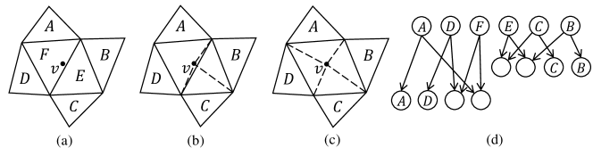
Figure 1: An example of the tracing structure. Here a point $v$ is added and the encroaching region contains triangles $E$ and $F$ (subfigure (a)). Four new triangles will be generated and replace the two previous triangles. They may or may not be created in the same round, and in this example this is done in two substeps (subfigures (b) and (c)). Part of the tracing structure is shown in subfigure (d). Four neighbor triangles $A$, $B$, $C$, and $D$ are copied, and four new triangles are created. An arrow indicates that a point is encroached by the head triangle only if it is encroached by the tail triangle.

We first construct the DT of the first $n/\log_{2}n$ points in the initial round using Algorithm 2 while building the tracing structure. Then at the beginning of each incremental round, each point traces down the structure to find its encroached triangles, and leaves itself in the encroached set of that triangle. Note that the encroached set for a given point might be large, but the average size across points is constant in expectation.

We now analyze the cost of finding all the encroached triangles when adding a set of new points. As discussed, the depth of $G$ is upper bounded by $O(\log n)$ whp. The number of encroached triangles of a point $x$ can be analyzed by considering the degree of the point (number of incident triangles) if added to the DT. By Euler’s formula, the average degree of a node in a planar graph is at most $6$. Since we add the points in a random order, the expected value of $|S(G,x)|$ in Theorem 3.1 is constant. Finally, the number of all encroached (including non-leaf) triangles of this point is upper bounded by the number of inCircle tests. Then $|R(G,x)|$, the expected number of visible vertices of $x$, is $O(\log n)$ (Theorem 4.2 in [16]).

After finding the encroached triangles for each point being added, we need to collect them together to add them to the triangle. This step can be done in parallel with a semisort, which takes linear expected work (writes) and $O(\log^{2}m)$ depth whp [34], where $m$ is the number of inserted points in this round. Combining these results leads to the following lemma.

Lemma 5.1.

Given $2m$ points in the plane and a tracing structure $T$ generated by Algorithm 2 on a randomly selected subset of $m$ points, computing for each triangle in $T$ the points that encroach it among the remaining $m$ points takes $O(m\log m+\omega{}m)$ work ($O(m)$ writes) and $O(\log^{2}n)$ depth whp in the Asymmetric NP model.

The idea of the algorithm is to keep doubling the size of the set that we add (i.e., prefix doubling). Each round applies Algorithm 2 to insert the points and build a tracing structure, and then the DAG tracing algorithm to locate the points for the next round. The depth of each round is upper bounded by the overall depth of the DAG on all points, which is $O(\log n)$ whp, where $n$ is the original size. We obtain the following theorem.

Theorem 5.1.

Planar Delaunay triangulation can be computed using $O(n\log n+\omega{}n)$ work (i.e., $O(n)$ writes) in expectation and $O(\log^{2}n\log\log n)$ depth whp on the Asymmetric NP model with priority-writes.

Proof.

The original Algorithm 2 in [16] has $O(\log^{2}n)$ depth whp. In the prefix-doubling approach, the depth of each round is no more than $O(\log^{2}n)$, and the algorithm has $O(\log\log n)$ rounds. The overall depth is hence $O(\log^{2}n\log\log n)$ depth whp.

The work bound consists of the costs from the initial round, and the incremental rounds. The initial round computes the triangulation of the first $n/\log_{2}n$ points, using at most $O(n)$ inCircle tests, $O(n)$ writes and $O(\omega{}n)$ work. For the incremental rounds, we have two components, one for locating encroached triangles in the tracing structure, and one for applying Algorithm 2 on those points to build the next tracing structure. The first part is handled by Lemma 5.1. For the second part we we can apply a similar analysis to Theorem 4.2 of [16]. In particular, the probability that there is a dependence from a triangle in the $i$’th point (in the random order) to a triangle added by a later point at location $j$ in the ordering is upper bounded by $24/i$. Summing across all points in the second half (we have already resolved the first half) gives:

$$\mathbb{E}[C]\leq\sum_{i=m+1}^{2m}\sum_{j=i+1}^{2m}24/i=O(m)\;.$$

This is a bound on both the number of reads and the number of writes. Since the points added in each round doubles, the cost is dominated by the last round, which is $O(n\log n)$ reads and $O(n)$ writes, both in expectation. Combined with the cost of the initial round gives the stated bounds. ∎

6 Space-Partitioning Data Structures

Space partitioning divides a space into non-overlapping regions. This process is usually applied repeatedly until the number of objects in a region is small enough, so that we can afford to answer a query in linear work within the region. We refer to the tree structure used to represent the partitioning as the space-partitioning tree. Commonly-used space-partitioning trees include binary space partitioning trees, quad/oct-trees, $k$-d trees, and their variants, and are widely used in computational geometry [26, 38], computer graphics [3], integrated circuit design, learning theory, etc.

In this section, we propose write-efficient construction and update algorithms for $k$-d trees [10]. We discuss how to support dynamic updates write-efficiently in Section 6.2, and we discuss how to apply our technique to other space-partitioning trees in Section 6.3.

6.1 $k$-d Tree Construction and Queries

$k$-d trees have many variants that facilitate different queries. We start with the most standard applications on range queries and nearest neighbor queries, and discussions for other queries are in Section 6.3. A range query can be answered in $O(n^{(k-1)/k})$ worst-case work, and an approximate $(1+\epsilon)$-nearest neighbor (ANN) query requires $\log n\cdot O(1/\epsilon)^{k}$ work assuming bounded aspect ratio, both in $k$-dimensional space. The tree to achieve these bounds can be constructed by always partitioning by the median of all of the objects in the current region either on the longest dimension of the region or cycling among the $k$ dimensions. The tree has linear size and $\log_{2}n$ depth [26], and can be constructed using $O(n\log n)$ reads and writes. We now discuss how to reduce the number of writes to $O(n)$.

One solution is to apply the incremental construction by inserting the objects into a $k$-d tree one by one. This approach requires linear writes, $O(n\log n)$ reads and polylogarithmic depth. However, the splitting hyperplane is no longer based on the median, but the object with the highest priority pre-determined by a random permutation. The expected tree depth can be $c\log_{2}n$ for $c>1$, but to preserve the range query cost we need the tree depth to be $\log_{2}n+O(1)$ (see details in Lemma 6.1). Motivated by the incremental construction, we propose the following variant, called $p$-batched incremental construction, which guarantees both write-efficiency and low tree depth.

The $p$-batched incremental construction. The $p$-batched incremental construction is a variant of the classic incremental construction where the dependence graph is a tree. Unlike the classic version, where the splitting hyperplane (splitter) of a tree node is immediately set when inserting the object with the highest priority, in the $p$-batched version, each leaf node will buffer at most $p$ objects before it determines the splitter. We say that a leaf node overflows if it holds more than $p$ objects in its buffer. We say that a node is generated when created by its parent, and settled after finding the splitters, creating leaves and pushing the objects to the leaves’ buffers.

The algorithm proceeds in rounds, where in each round it first finds the corresponding leaf nodes that the inserted objects belong to, and adds them into the buffers of the leaves. Then it settles all of the overflowed leaves, and starts a new round. An illustration of this algorithm is shown in Figure 2. After all objects are inserted, the algorithm finishes building the subtree of the tree nodes with non-empty buffers recursively. For write-efficiency, we require the small-memory size to be $\Omega(p)$, and the reason will be shown in the cost analysis.

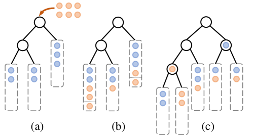
Figure 2: An illustration of one round in the $p$-batched incremental construction for $p=4$. Subfigure (a) shows the initial state of this round. Then the new objects (shown in orange) are added to the buffers in the leaves, as shown in subfigure (b). Two of the buffers overflow, and so we settle these two leaves as shown in subfigure (c).

We make a partition once we have gathered $p$ objects in the corresponding subregion based on the median of these $p$ objects. When $p=1$, the algorithm is the incremental algorithm mentioned above, but the range query cost cannot be preserved. When $p=n$, the algorithm constructs the same tree as the classic $k$-d tree construction algorithm, but requires more than linear writes unless the small-memory size is $O(n)$, which is impractical when $n$ is large. We now try to find the smallest value of $p$ that preserves the query cost, and we analyze the cost bounds accordingly.

Range query. We use the following lemma to analyze the cost of a standard $k$-d range query (on an axis-aligned hypercube for $k\geq 2$).

Lemma 6.1.

A $k$-d range query costs $O(2^{((k-1)/k)h})$ using our $k$-d tree of height $h$.

Proof Sketch.

A $k$-d range query has at most $2k$ faces that generate $2k$ half-spaces, and we analyze the query cost of each half-space. Since each axis is partitioned once in every $k$ consecutive levels, one side of the partition hyperplane perpendicular to the query face will be either entirely in or out of the associated half-space. We do not need to traverse that subtree (we can either directly report the answer or ignore it). Therefore every $k$ levels will expand the search tree by a factor of at most $2^{k-1}$. Thus the query cost is $O(2^{((k-1)/k)h})$. ∎

Lemma 6.2.

For our $p$-batched $k$-d tree, $p=\Omega(\log^{3}n)$ guarantees the tree height to be no more than $\log_{2}n+O(1)$ whp.

Proof.

We now consider the $p$-batched incremental construction. Since we are partitioning based on the median of $p$ random objects, the hyperplane can be different from the actual median. To get the same cost bound, we want the actual number of objects on the two sides to differ by no more than a factor of $\epsilon$ whp. Since we pick $p$ random samples, by a Chernoff bound the probability that more than $1/2p$ samples are within the first $(1/2-\epsilon/4)n$ objects is upper bounded by $e^{-p\epsilon^{2}/24}$. Hence, the probability that the two subtree weights of a tree node differ by more than a factor of $\epsilon$ is no more than $2e^{-p\epsilon^{2}/24}$. This $\epsilon$ controls the tree depth, and based on the previous analysis we want to have $n(\frac{1}{2}+\frac{\epsilon}{4})^{\log_{2}n/p+O(1)}<p$. Namely, we want the tree to have no more than $\log_{2}n/p+O(1)$ levels whp to reach the subtrees with less than $p$ elements, so the overall tree depth is bounded by $\log_{2}n/p+O(1)+\log_{2}p=\log_{2}n+O(1)$. Combining these constraints leads to $\epsilon=O(1)/\log_{2}n$ and $p=\Omega(\log^{3}n)$. ∎

Lemma 6.2 indicates that setting $p=\Omega(\log^{3}n)$ gives a tree height of $\log_{2}n+O(1)$ whp, and Lemma 6.1 shows that the corresponding range query cost is $O(2^{((k-1)/k)(O(1)+\log_{2}n)})=O(n^{(k-1)/k})$, matching the standard range query cost.

ANN query. If we assume that the input objects are well-distributed and the $k$-d tree satisfies the bounded aspect ratio, then the cost of a $(1+\epsilon)$-ANN query is proportional to the tree height. As a result, $p=\Omega(\log n)$ leads to a query cost of $\log n\cdot O(1/\epsilon)^{k}$ whp.

Parallel construction and cost analysis. To get parallelism, we use the prefix-doubling approach, starting with $n/\log n$ objects in the first round. The number of reads of the algorithm is still $\Theta(n\log n)$, since it is lower bounded by the cost of sorting when $k=1$, and upper bounded by $O(n\log n)$ since the modified algorithm makes asymptotically no more comparisons than the classic implementation. We first present the following lemma.

Lemma 6.3.

When a leaf overflows at the end of a round, the number of objects in its buffer is $O(p)$ whp when $p=\Omega(\log n)$.

Proof Sketch.

In the previous round, assume $n^{\prime}$ objects were in the tree. At that time no more than $p-1$ objects are buffered in this leaf node. Then in the current round another $n^{\prime}$ objects are inserted, and by a Chernoff bound, the probability that the number of objects falling into this leaf node is more than $(c+1)p$ is at most $e^{-{c^{2}p/2}}$. Plugging in $p=\Omega(\log n)$ proves the lemma. ∎

We now bound the parallel depth of this construction. The initial round runs the standard construction algorithm on the first $n/\log_{2}n$ objects, which requires $O((\log^{2}p+\log n)\log n)=O(\log^{2}n)$ depth. Then in each of the next $O(\log\log n)$ incremental rounds, we need to locate leaf nodes and a parallel semisort to put the objects into their buffers. Both steps can be done in $O(\log^{2}n)$ depth whp [34]. Then we also need to account for the depth of settling the leaves after the incremental rounds. When a leaf overflows, by Lemma 6.3 we need to split a set of $O(p)$ objects for each leaf, which has a depth of $O(\log^{2}p)=O(\log\log n)$ using the classic approach, and is applied for no more than a constant number of times whp by Lemma 6.3.

We now analyze the number of writes this algorithm requires. The initial round requires $O(n)$ writes as it uses a standard construction algorithm on $n/\log_{2}n$ objects. In the incremental rounds, $O(1)$ writes whp are required for each object to find the leaf node it belongs to and add itself to the buffer using semisorting [34]. From Lemma 6.3, when finding the splitting hyperplane and splitting the object for a tree node, the number of writes required is $O(p)$ whp. Note that after a new leaf node is generated from a split, it contains at least $p/2$ objects. Therefore, after all incremental rounds, the tree contains at most $O(n/p)$ tree nodes, and the overall writes to generate them is $O((n/p)\cdot p)=O(n)$. After the incremental rounds finish, we need $O(n)$ writes to settle the leaves with non-empty buffers, assuming $O(p)$ cache size. In total, the algorithm uses $O(n)$ writes whp.

Theorem 6.1.

A $k$-d tree that supports range and ANN queries efficiently can be computed using $O(n\log n+\omega{}n)$ expected work (i.e., $O(n)$ writes) and $O(\log^{2}n)$ depth whp in the Asymmetric NP model. For range query the small-memory size required is $\Omega(\log^{3}n)$.

6.2 $k$-d Tree Dynamic Updates

Unlike many other tree structures, we cannot rotate the tree nodes in $k$-d trees since each tree node represents a subspace instead of just a set of objects. Deletion is simple for $k$-d trees, since we can afford to reconstruct the whole structure from scratch when a constant fraction of the objects in the $k$-d tree have been removed, and before the reconstruction we just mark the deleted node (constant reads and writes per deletion via an unordered map). In total, the amortized cost of each deletion is $O(\omega{}+\log n)$. For insertions, we discuss two techniques that optimize either the update cost or the query cost.

Logarithmic reconstruction [46]. We maintain at most $\log_{2}n$ $k$-d trees of sizes that are increasing powers of $2$. When an object is inserted, we create a $k$-d tree of size $1$ containing the object. While there are trees of equal size, we flatten them and replace the two trees with a tree of twice the size. This process keeps repeating until there are no trees with the same size. When querying, we search in all (at most $\log_{2}n$) trees. Using this approach, the number of reads and writes on an insertion is $O(\log^{2}n)$, and on a deletion is $O(\log n)$. The costs for range queries and ANN queries are $O(n^{(k-1)/k})$ and $\log^{2}n\cdot O(1/\epsilon)^{k}$ respectively, plus the cost for writing the output.

If we apply our write-efficient $p$-batched version when reconstructing the $k$-d trees, we can reduce the writes (but not reads) by a factor of $O(\log n)$ (i.e., $O(\log n)$ and $O(1)$ writes per update).

When using logarithmic reconstruction, querying up to $O(\log n)$ trees can be inefficient in some cases, so here we show an alternative solution that only maintains a single tree.

Single-tree version. As discussed in Section 6.1, only the tree height affects the costs for range queries and ANN queries. For range queries, Lemma 6.2 indicates that the tree height should be $\log_{2}n+O(1)$ to guarantee the optimal query cost. To maintain this, we can tolerate an imbalance between the weights of two subtrees by a factor of $O(1/\log n)$, and reconstruct the subtree when the imbalance is beyond the constraint. In the worst case, a subtree of size $n^{\prime}$ is rebuilt once after $O(n^{\prime}/\log n)$ insertions into the subtree. Since the reconstructing a subtree of size $n^{\prime}$ requires $O(n^{\prime}\log n^{\prime}+\omega{}n^{\prime})$ work, each inserted object contributes $O(\log n\log n^{\prime}+\omega{}\log n)$ work to every node on its tree path, and there are $O(\log n)$ such nodes. Hence, the amortized work for an insertion is $O(\log^{3}n+\omega{}\log^{2}n)$. For efficient ANN queries, we only need the tree height to be $O(\log n)$, which can be guaranteed if the imbalance between two subtree sizes is at most a constant multiplicative factor. Using a similar analysis, in this case the amortized work for an insertion is $O(\log^{2}n+\omega{}\log n)$.

6.3 Extension to Other Trees and Queries

In Section 6.1 we discussed the write-efficient algorithm to construct a $k$-d tree that supports range and ANN queries. $k$-d trees are also used in many other queries in real-world applications, such as ray tracing, collision detection for non-deformable objects, $n$-body simulation, and geometric culling (using BSP trees). The partition criteria in these applications are based on some empirical heuristics (e.g., the surface-area heuristic [30]), which generally work well on real-world instances, but usually with no theoretical guarantees.

The $p$-batched incremental construction can be applied to these heuristics, as long as each object contributes linearly to the heuristic. Let us consider the surface-area heuristic [30] as an example, which does an axis-aligned split and minimizes the sum of the two products of the subtree’s surface area and the number of objects. Instead of sorting the coordinates of all objects in this subtree and finding the optimal split point, we can do approximately by splitting when at least $p$ of the objects are inserted into a region. When picking a reasonable value of $p$ (like $O(\log^{2}n)$ or $O(\log^{3}n)$), we believe the tree quality should be similar to the exact approach (which is a heuristic after all). However, the $p$-batched approach does not apply to heuristics that are not linear in the size of the object set. Such cases happen in the Callahan-Kosaraju algorithm [20] when the region of each $k$-d tree node shrinks to the minimum bounding box, or the object-partitioning data structures (like R-trees or bounding volume hierarchies) where each object can contribute arbitrarily to the heuristic.

7 Augmented Trees

An augmented tree is a tree that keeps extra data on each tree node other than what is used to maintain the balance of this tree. We refer to the extra data on each tree node as the augmentation. In this section, we introduce a framework that gives new algorithms for constructing both static and dynamic augmented trees including interval trees, 2D range trees, and priority search trees that are parallel and write-efficient. Using these data structures we can answer 1D stabbing queries, 2D range queries, and 3-sided queries (defined in Section 7.1). For all three problems, we assume that the query results need to be written to the large-memory. Our results are summarized in Table 1. We improve upon the traditional algorithms in two ways. First, we show how to construct interval trees and priority search trees using $O(n)$ instead of $O(n\log n)$ writes (since the 2D range tree requires $O(n\log n)$ storage we cannot asymptotically reduce the number of writes). Second, we provide a tradeoff between update costs and query costs in the dynamic versions of the data structures. The cost bounds are parameterized by $\alpha$. By setting $\alpha=O(1)$ we achieve the same cost bounds as the traditional algorithms for queries and updates. $\alpha$ can be chosen optimally if we know the update-to-query ratio $r$. For interval and priority trees, the optimal value of $\alpha$ is $\min(2+\omega{}/r,\omega{})$. The overall work without considering writing the output can be improved by a factor of $\Theta(\log\alpha)$. For 2D range trees, the optimal value of $\alpha$ is $2+\min(\omega{}/r,\omega{})/\log_{2}n$.

	Construction	Query	Update
Classic interval tree	$O(\omega n\log n)$	$O(\omega k+\log n)$	$O(\omega{}\log n)$
Our interval tree	$O(\omega n+n\log n)$	$O(\omega k+\alpha\log_{\alpha}n)$	$O((\omega+\alpha)\log_{\alpha}n)$
Classic priority search tree	$O(\omega n\log n)$	$O(\omega k+\log n)$	$O(\omega{}\log n)$
Our priority search tree	$O(\omega n+n\log n)$	$O(\omega k+\alpha\log_{\alpha}n)$	$O((\omega+\alpha)\log_{\alpha}n)$
Classic range Tree	$O(\omega n\log n)$	$O(\omega k+\log^{2}n)$	$O((\log n+\omega)\log n)$
Our range tree	$O((\alpha+\omega)\,n\log_{\alpha}n)$	$O(\omega k+\alpha\log_{\alpha}n\,{\log n})$	$O((\alpha\log n+\omega)\log_{\alpha}n)$

Table 1: A summary of the work cost of the data structures discussed in Section 7. In all cases, we assume that the tree contains $n$ objects (intervals or points). For interval trees and priority search trees, we can reduce the number of writes in the construction from $O(\log n)$ per element to $O(1)$. For dynamic updates, we can reduce the number of writes per update by a factor of $\Theta(\log\alpha)$ at the cost of increasing the number of reads in update and queries by a factor of $\alpha$ for any $\alpha\geq 2$.

We discuss two techniques in this section that we use to achieve write-efficiency. The first technique is to decouple the tree construction from sorting, and we introduce efficient algorithms to construct interval and priority search trees in linear reads and writes after the input is sorted. Sorting can be done in parallel and write-efficiently (linear writes).Using this approach, the tree structure that we obtain is perfectly balanced.

The second technique that we introduce is the $\alpha$-labeling technique. We mark a subset of tree nodes as critical nodes by a predicate function parameterized by $\alpha$, and only maintain augmentations on these critical nodes. We can then guarantee that every update only modifies $O(\log_{\alpha}n)$ nodes, instead of $O(\log n)$ nodes as in the classic algorithms. At a high level, the $\alpha$-labeling is similar to the weight-balanced B-tree (WBB tree) proposed by Arge et al. [5, 6] for the external-memory (EM) model [1]. However, as we discuss in Section 7.3, directly applying the EM algorithms [5, 6, 2, 53, 52] does not give us the desired bounds in our model. Secondly, our underlying tree is still binary. Hence, we mostly need no changes to the algorithmic part that dynamically maintains the augmentation in this trees, but just relax the balancing criteria so the underlying search trees can be less balanced. An extra benefit of our framework is that bulk updates can be supported in a straightforward manner. Such bulk updates seem complicated and less obvious in previous approaches. We propose algorithms on our trees that can support bulk updates write-efficiently and in polylogarithmic depth.

The rest of this section is organized as follows. We first provide the problem definitions and review previous results in Section 7.1. Then in Section 7.2, we introduce our post-sorted construction technique for constructing interval and priority search trees using a linear number of writes. Finally, we introduce the $\alpha$-labeling technique to support a tradeoff in query and update cost for interval trees, priority search trees, and range trees in Section 7.3.

7.1 Preliminaries and Previous Work

We define the weight or size of tree node or a subtree as the number of nodes in this subtree plus one. The “plus one” guarantees that the size of a tree node is always the sum of the sizes of its two children, which simplifies our discussion. This is also the standard balancing criteria used for weight-balanced trees [45].

Interval trees and the 1D stabbing queries. An interval tree [26, 27, 42] organizes a set of $n$ intervals $S=\{s_{i}=(l_{i},r_{i})\}$ defined by their left and right endpoints. The key on the root of the interval tree is the median of the $2n$ endpoints. This median divides all intervals into two categories: those completely on its left/right, which then form the left/right subtrees recursively, and those covering the median, which are stored in the root. The intervals in the root are stored in two lists sorted by the left and right endpoints respectively. In this paper, we use red-black trees to maintain such ordered lists to support dynamic updates and refer to them as the inner trees. In the worst case, the previous construction algorithms scan and copy $O(n)$ intervals in $O(\log n)$ levels, leading to $O(n\log n)$ reads and writes.

The interval tree can be used to answer a 1D stabbing query: given a set of intervals, report a list of intervals covering the specific query point $p_{q}$. This can be done by searching $p_{q}$ in the tree. Whenever $p_{q}$ is smaller (larger) than the key of the current node, all intervals in the current tree node with left (right) endpoints smaller than $p_{q}$ should be reported. This can be done efficiently by scanning the list sorted by left (right) endpoints. The overall query cost is $O(\omega k+\log n)$ (where $k$ is the output size).

2D Range trees and the 2D range queries. The 2D range tree [11] organizes a set of $n$ points $p=\{p_{i}=(x_{i},y_{i})\}$ on the 2D plane. It is a tree structure augmented with an inner tree, or equivalently, a two-level tree structure. The outer tree stores every point sorted by their $x$-coordinate. Each node in the outer tree is augmented with an inner tree structure, which contains all the points in its subtree, sorted by their y-coordinate.

The 2D range tree can be used to answer the 2D range query: given $n$ points in the 2D plane, report the list of points with $x$-coordinate between $x_{L}$ and $x_{R}$, and $y$-coordinate between $y_{B}$ and $y_{T}$. Such range queries using range trees can be done by two nested searches on $(x_{L},x_{R})$ in the outer tree and $(y_{B},y_{T})$ in at most $O(\log n)$ associated inner trees. Using balanced BSTs for both the inner and outer trees, a range tree can be constructed with $O(n\log n)$ reads and writes, and each query takes $O(\log^{2}n+k)$ reads and $O(k)$ writes (where $k$ is the output size). A range tree requires $O(n\log n)$ storage so the number of writes for construction is already optimal.

Priority search trees and 3-sided range queries. The priority search tree [43, 26] (priority tree for short) contains a set of $n$ points $p=\{p_{i}=(x_{i},y_{i})\}$ each with a coordinate ($x_{i}$) and a priority ($y_{i}$). There are two variants of priority trees, one is a search tree on coordinates that keeps a heap order of the priorities as the augmented values [43, 5]. The other one is a heap of the priorities, where each node is augmented with a splitter between the left and right subtrees on the coordinate dimension [43, 26]. The construction of both variants uses $O(n\log n)$ reads and writes as shown in the original papers [43, 26]. For example, consider the second variant. The root of a priority tree stores the point with the highest priority in $p$. All the other points are then evenly split into two sets by the median of their coordinates which recursively form the left and right subtrees. The construction scans and copies $O(n)$ points in $O(\log n)$ levels, leading to $O(n\log n)$ reads and writes for the construction.

Many previous results on dynamic priority search trees use the first variant because it allows for rotation-based updates. In this paper, we discuss how to construct the second variant allowing reconstruction-based updates, since it is a natural fit for our framework. We also show that bulk updates can be done write-efficiently in this variant. For the rest of this section, we discuss the second variant of the priority tree.

The priority tree can be used to answer the 3-sided queries: given a set of $n$ points, report all points with coordinates in the range $[x_{L},x_{R}]$, and priority higher than $y_{B}$. This can be done by traversing the tree, skipping the subtrees whose coordinate range do not overlap $[x_{L},x_{R}]$, or where the priority in the root is lower than $y_{B}$. The cost of each query is $O(\omega{}k+\log n)$ for an output of size $k$ [26].

7.2 The Post-Sorted Construction

For interval trees and priority search trees, the standard construction algorithms [26, 25, 27, 42, 43] require $O(n\log n)$ reads and writes, even though the output is only of linear size. This section describes algorithms for constructing them in an optimal linear number of writes. Both algorithms first sort the input elements by their $x$-coordinate in $O(\omega n+n\log n)$ work and $O(\log^{2}n)$ depth using the write-efficient comparison sort described in Section 4. We now describe how to build the trees in $O(n)$ reads and writes given the sorted input. For a range tree, since the standard tree has $O(n\log n)$ size, the classic construction algorithm is already optimal.

Interval Tree. After we sort all $2n$ coordinates of the endpoints, we can first build a perfectly-balanced binary search tree on the endpoints using $O(n)$ reads and writes and $O(\log n)$ depth. We now consider how to construct the inner tree of each tree node.

We create a lowest common ancestor (LCA) data structure on the keys of the tree nodes that allows for constant time queries. This can be constructed in $O(n)$ reads/writes and $O(\log^{2}n)$ depth [12, 40]. Each interval can then find the tree node that it belongs to using an LCA query on its two endpoints. We then use a radix sort on the $n$ intervals. The key of an interval is a pair with the first value being the index of the tree node that the interval belongs to, and the second value being the index of the left endpoint in the pre-sorted order. The sorted result gives the interval list for each tree node sorted by left endpoints. We do the same for the right endpoints. This step takes $O(n)$ reads/writes overall. Finally, we can construct the inner trees from the sorted intervals in $O(n)$ reads/writes across all tree nodes.

Parallelism is straightforward for all steps except for the radix sort. The number of possible keys can be $O(n^{2})$, and it is not known how to radix sort keys from such a range work-efficiently and in polylogarithmic depth. However, we can sort a range of $O(n\log n)$ in $O(\omega n)$ expected work and $O(\log^{2}n)$ depth whp [48]. Hence our goal is to limit the first value into a $O(\log n)$ range. We note that given the left endpoint of an interval, there are only $\log_{2}(2n)$ possible locations for the tree node (on the tree path) of this interval. Therefore instead of using the tree node as the first value of the key, we use the level of the tree node, which is in the range $[1,\ldots,O(\log n)]$. By radix sorting these pairs, so we have the sorted intervals (based on left or right endpoint) for each level. We observe that the intervals of each tree node are consecutive in the sorted interval list per level. This is because for tree nodes $u_{1}$ and $u_{2}$ on the same level where $u_{1}$ is to the left of $u_{2}$, the endpoints of $u_{1}$’s intervals must all be to the left of $u_{2}$’s intervals. Therefore, in parallel we can find the first and the last intervals of each node in the sorted list, and construct the inner tree of each node. Since the intervals are already sorted based on the endpoints, we can build inner trees in $O(n)$ reads and writes and $O(\log^{2}n)$ depth [13].

Priority Tree. In the original priority tree construction algorithm, points are recursively split into sub-problems based on the median at each node of the tree. This requires $O(n)$ writes at each level of the tree if we explicitly copy the nodes and pack out the root node that is removed. To avoid explicit copying, since the points are already pre-sorted, our write-efficient construction algorithm passes indices determining the range of points belonging to a sub-problem instead of actually passing the points themselves. To avoid packing, we simply mark the position of the removed point in the list as invalid, leaving a hole, and keep track of the number of valid points in each sub-problem.

Our recursive construction algorithm works as follows. For a tree node, we know the range of the points it represents, as well as the number of valid points $n_{v}$. We then pick the valid point with the highest priority as the root, mark the point as invalid, find the median among the valid points, and pass the ranges based on the median and number of valid points (either $\lfloor(n_{v}-1)/2\rfloor$ or $\lceil(n_{v}-1)/2\rceil$) to the left and right sub-trees, which are recursively constructed. The base case is when there is only one valid point remaining, or when the number of holes is more than the valid points. Since each node in the tree can only cause one hole, for every range corresponding to a node, there are at most $O(\log n)$ holes. Since the size of the small-memory is $\Omega(\log n)$, when the number of valid points is fewer than the number of holes, we can simply load all of the valid points into the small-memory and construct the sub-tree.

To efficiently implement this algorithm, we need to support three queries on the input list: finding the root, finding the $k$-th element in a range (e.g., the median), and deleting an element. All queries and updates can be supported using a standard tournament tree where each interior node maintains the minimum element and the number of valid nodes within the subtree. With a careful analysis, all queries and updates throughout the construction require linear reads/writes overall. The details are provided in Appendix A.

The parallel depth is $O(\log^{2}n)$—the bottleneck lies in removing the points. There are $O(\log n)$ levels in the priority tree and it costs $O(\log n)$ writes for removing elements from the tournament tree on each level. For the base cases, it takes linear writes overall to load the points into the small-memory and linear writes to generate all tree nodes. The depth is $O(\log n)$.

We summarize our result in this section in Theorem 7.1.

Theorem 7.1.

An interval tree or a priority search tree can be constructed with pre-sorted input in $O(\omega{}n)$ expected work and $O(\log^{2}n)$ depth whp on the Asymmetric NP model.

7.3 Dynamic Updates using Reconstruction-Based Rebalancing

Dynamic updates (insertions and deletions) are often supported on augmented trees [26, 25, 27, 42, 43] and the goal of this section is to support updates write-efficiently, at the cost of performing extra reads to reduce the overall work. Traditionally, an insertion or deletion costs $O(\log n)$ for interval trees and priority search trees, and $O(\log^{2}n)$ for range trees. In the asymmetric setting, the work is multiplied by $\omega{}$. To reduce the overall work, we introduce an approach to select a subset of tree nodes as critical nodes, and only update the balance information of those nodes (the augmentations are mostly unaffected). The selection of these critical nodes are done by the $\alpha$-labeling introduced in Section 7.3.1. Roughly speaking, for each tree path from the root to a leaf node, we have $O(\log_{\alpha}n)$ critical nodes marked such that the subtree weights of two consecutive marked nodes differ by about a factor of $\alpha\geq 2$. By doing so, we only need to update the balancing information in the critical nodes, leading to fewer tree nodes modified in an update.

Arge et al. [5, 6] use a similar strategy to support dynamic updates on augmented trees in the external-memory (EM) model, in which a block of data can be transferred in unit cost [1]. They use a $B$-tree instead of a binary tree, which leads to a shallower tree structure and fewer memory accesses in the EM model. However, in the Asymmetric NP model, modifying a block of data requires work proportional to the block size, and directly using their approach cannot reduce the overall work. Inspired by their approach, we propose a simple approach to reduce the work of updates for the Asymmetric NP model.

The main component of our approach is reconstruction-based rebalancing using the $\alpha$-labeling technique. We can always obtain the sorted order via the tree structure, so when imbalance occurs, we can afford to reconstruct the whole subtree in reads and writes proportional to the subtree size and polylogarithmic depth. This gives a unified approach for different augmented trees: interval trees, priority search trees, and range trees.

We introduce the $\alpha$-labeling idea in Section 7.3.1, the rebalancing algorithm in Section 7.3.2, and its work analysis in Section 7.3.3. We then discuss the maintenance of augmented values for different applications in Section 7.3.4. We mention how to parallelize bulk updates in Section 7.3.5.

7.3.1 $\alpha$-Labeling

The goal of the $\alpha$-labeling is to maintain the balancing information at only a subset of tree nodes, the critical nodes, such that the number of writes per update is reduced. Once the augmented tree is constructed, we label the node as a critical node if for some integer $i\geq 0$, (1) its subtree weight is between $2\alpha^{i}$ and $4\alpha^{i}-2$ (inclusive); or (2) its subtree weight is $2\alpha^{i}-1$ and its sibling’s subtree weight is $2\alpha^{i}$. All other nodes are secondary nodes. As a special case, we always treat the root as a virtual critical node, but it does not necessary satisfy the invariants of critical nodes. Note that all leaf nodes are critical nodes in $\alpha$-labeling since they always have subtrees of weight 2. When we label a critical node, we refer to its current subtree weight (which may change after insertions/deletions) as its initial weight. Note that after the augmented tree is constructed, we can find and mark the critical nodes in $O(n)$ reads/writes and $O(\log n)$ depth. After that, we only maintain the subtree weights for these critical nodes, and use their weights to balance the tree.

Fact 7.2.

For a critical node $A$, $2\alpha^{i}-1\leq|A|\leq 4\alpha^{i}-2$ holds for some integer $i$.

This fact directly follows the definition of the critical node.

For two critical nodes $A$ and $B$, if $A$ is $B$’s ancestor and there is no other critical node on the tree path between them, we refer to $B$ as $A$’s critical child, and $A$ as $B$’s critical parent. We define a critical sibling accordingly.

We show the following lemma on the initial weights.

Lemma 7.1.

For any two critical nodes $A$ and $B$ where $A$ is $B$’s critical parent, their initial weights satisfy $\max\{(\alpha/2)|B|,2|B|-1\}\leq|A|\leq(2\alpha+1)|B|$.

Proof.

Based on Fact 7.2, we assume $2\alpha^{i}-1\leq|A|\leq 4\alpha^{i}-2$ and $2\alpha^{j}-1\leq|B|\leq 4\alpha^{j}-2$ for some integers $i$ and $j$. We first show that $i=j+1$. It is easy to check that $j$ cannot be larger than or equal to $i$. Assume by contradiction that $j<i-1$. With this assumption, we will show that there exists an ancestor of $B$, which we refer to it as $y$, which is a critical node. The existence of $y$ contradicts the fact that $A$ is $B$’s critical parent. We will use the property that for any tree node $x$ the weight of its parent $p(x)$ is $2|x|-1\leq|p(x)|\leq 2|x|+1$.

Assume that $B$ does not have such an ancestor $y$. Let $z$ be the ancestor of $B$ with weight closest to but no more than $2\alpha^{i-1}$. We consider two cases: (a) $|z|\leq 2\alpha^{i-1}-2$ and (b) $|z|=2\alpha^{i-1}-1$. In case (a) $z$’s parent $p(z)$ has weight at most $2|z|+1=4\alpha^{i-1}-3$. $|p(z)|$ cannot be less than $2\alpha^{i-1}$ by definition of $z$, and so $y=p(z)$, leading to a contradiction. In case (b), $z$’s sibling does not have weight $2\alpha^{i-1}$, otherwise $y=z$. However, then $|p(z)|\leq 2|z|=4\alpha^{i-1}-2$, and either $z$ is not the ancestor with weight closest to $2\alpha^{i-1}$ or $y=p(z)$.

Given $i=j+1$, we have $(\alpha/2)|B|\leq|A|\leq(2\alpha+1)|B|$ (by plugging in $2\alpha^{i}-1\leq|A|\leq 4\alpha^{i}-2$ and $2\alpha^{i-1}-1\leq|B|\leq 4\alpha^{i-1}-2$). Furthermore, since $A$ is $B$’s ancestor, we have $2|B|-1\leq|A|$. Combining the results proves the lemma. ∎

7.3.2 Rebalancing Algorithm based on $\alpha$-Labeling

We now consider insertions and deletions on an augmented tree. Maintaining the augmented values on the tree are independent of our $\alpha$-labeling technique, and differs slightly for each of the three tree structures. We will further discuss how to maintain augmented values in Section 7.3.4.

We note that deletions can be handled by marking the deleted objects without actually applying the deletion, and reconstructing the whole subtree once a constant fraction of the objects is deleted. Therefore in this section, we first focus on the insertions only. We analyze single insertions here, and discuss bulk insertions later in Section 7.3.5. Once the subtree weight of a critical node $A$ reaches twice the initial weight $s$, we reconstruct the whole subtree, label the critical nodes within the subtree, and recalculate the initial weights of the new critical nodes. An exception here is that, if $s\leq 4\alpha^{i}-2$ and $2\alpha^{i+1}-1\leq 2s$ for a certain $i$, we do not mark the new root since otherwise it violates the bound stated in Lemma 7.2 (see more details in Section 7.3.3) with $A$’s critical parent. After this reconstruction, $A$’s original critical parent gets one extra critical child, and the two affected children now have initial weights the same as $A$’s initial weight. If imbalance occurs at multiple levels, we reconstruct the topmost tree node. An illustration of this process is shown in Figure 3.

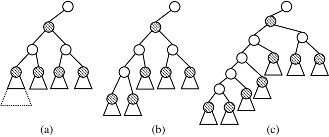
Figure 3: An illustration of rebalancing based on $\alpha$-labeling. The critical nodes are shaded. The case after construction is shown in (a) with solid borders. After some insertions, the size of one of the subtrees grows to twice its initial weight (dashed lines in (a)), so the algorithm reconstructs the subtree, as shown in (b). As we keep inserting new nodes along the left spine, the tree will look like what is shown in (c), but Lemma 7.2 guarantees that the subtree of the topmost critical node will be reconstructed before it gets more than $4\alpha+2$ critical children. The lemma also guarantees that on the path from a critical node to any of its critical children, there can be at most $4\alpha-1$ secondary nodes.

We can directly apply the algorithms in Section 7.2 to reconstruct a subtree as long as we have the sorted order of the (end)points in this subtree. For interval and range trees, we can acquire the sorted order by traversing the subtree. using linear work and $O(\log n)$ depth [51, 9]. For priority trees, since the tree nodes are not stored in-order, we need to insert all interior nodes into the tree in a bottom-up order based on their coordinates (without applying rebalancing) to get the total order on coordinates of all points (the details and cost analysis can be found in Appendix A). After we have the sorted order, a subtree of weight $n$ can be constructed in $O(\omega n)$ work and $O(\log^{2}n)$ depth.

As mentioned, we always treat the root as a virtual critical node, but it does not necessary satisfy the invariants of critical nodes. By doing so, once the weight of the whole tree doubles, we reconstruct the entire tree. We need $\Omega(n)$ insertions for one reconstruction on the root (there can be deletions). The cost for reconstruction is $O(\omega{}n)$ for interval trees and priority trees, and $O(\omega n\log_{\alpha}n)$ for range trees (shown in Section 7.3.4). The amortized cost is of a lower order compared to the update cost shown in Theorem 7.4.

7.3.3 Cost Analysis of the Rebalancing

To show the rebalancing cost, we first prove some properties about our dynamic augmented trees.

Lemma 7.2.

In a dynamic augmented tree with $\alpha$-labeling, we have $\max\{(\alpha/4)|B|,(3/2)|B|-1\}\leq|A|\leq(4\alpha+2)|B|$ for any two critical nodes $A$ and $B$ where $A$ is $B$’s critical parent.

Proof.

For any critical node $A$ in the tree, the subtree weight of its critical child $B$ can grow up to a factor of 2 of $B$’s initial weight, after which the subtree is reconstructed to two new critical nodes with the same initial weight of $B$. $A$’s weight can grow up to a factor of 2 of $A$’s initial weight, without affecting $B$’s weight (i.e., all insertions occur in $A$’s other critical children besides $B$). Combining these observations with the result in Lemma 7.1 shows this lemma except for the $(3/2)|B|-1\leq|A|$ part. Originally we have $2|B|-1\leq|A|$ after the previous reconstruction. $|A|$ grows together when $|B|$ grows, and right before the reconstruction of $B$ we have $(3/2)|B|-1\leq|A|$. ∎

Lemma 7.2 shows that each critical node has at most $4\alpha+2$ critical children, and so that there are at most $4n+1$ secondary nodes to connect them. This leads to the following corollary.

Corollary 7.1.

The length of the path from a critical node to its critical parent is at most $4\alpha+1$.

Combining Lemma 7.2 and Corollary 7.1 gives the following result.

Corollary 7.2.

For a leaf node in a tree with $\alpha$-labeling, the tree path to the root contains $O(\log_{\alpha}n)$ critical nodes and $O(\alpha\log_{\alpha}n)$ nodes.

Corollary 7.2 shows the number of reads during locating a node in an augmented tree, and the number of critical nodes on that path.

With these results, we now analyze the cost of rebalancing for each insertion. For a critical node with initial weight $W$, we need to insert at least another $W$ new nodes into this subtree before the next reconstruction of this critical node. Theorem 7.1 shows that the amortized cost for each insertion in this subtree is therefore $O(\omega{})$ on this node. Based on Corollary 7.2, the amortized cost for each insertion contains $O(\log_{\alpha}n)$ writes and $O(\alpha\log_{\alpha}n)$ reads. In total, the work per insertion is $O((\alpha+\omega)\log_{\alpha}n)$, since we need to traverse $O(\alpha\log_{\alpha}n)$ tree nodes, update $O(\log_{\alpha}n)$ subtree weights, and amortize $O(\omega\log_{\alpha}n)$ work for reconstructions.

We note that any interleaving insertions can only reduce the amortized cost for deletions. Therefore, both the algorithm and the bound can be extended to any interleaving sequence of insertions and deletions. Altogether, we have the following result, which may be of independent interest.

Theorem 7.3.

Using reconstruction-based rebalancing based on the $\alpha$-labeling technique, the amortized cost of each update (insertion or deletion) to maintain the balancing information on a tree of size $n$ is $O((\omega{}+\alpha)\log_{\alpha}n)$.

7.3.4 Handling Augmented Values

Since the underlying tree structure is still binary, minor changes to the trees are required for different augmentations.

Interval trees.

We do not need any changes for the interval tree. Since we never apply rotations, we directly insert/delete the interval in the associated inner tree with a cost of $O(\log n+\omega{})$.

Range trees.

For the range tree, we only keep the inner trees for the critical nodes. As such, the overall augmentation weight (i.e., overall weights of all inner trees) is $O(n\log_{\alpha}n)$. For each update, we insert/delete this element in $O(\log_{\alpha}n)$ inner trees (Corollary 7.2), and the overall cost is $O((\log n+\omega{})\log_{\alpha}n)$. Then each query may look into no more than $O(\alpha\log_{\alpha}n)$ inner trees each requiring $O(\log n)$ work for a 1D range query. The overall cost for a query is therefore $O(\omega{}k+\alpha\log_{\alpha}n\log n)$.

Priority trees.

For insertions on priority trees, we search its coordinate in the tree and put it where the current tree node is of lower priority than the new point. The old subtree root is then recursively inserted to one of its subtrees. The cost can be as expensive as $O(\omega\alpha\log_{\alpha}n)$ when a point with higher priority than all tree nodes is inserted. To address this, points are only stored in the critical nodes, and the secondary nodes only partition the range, without holding points as augmented values. This can be done by slightly modifying the construction algorithm in Section 7.2. During the construction, once the current node is a secondary node, we only partition the range, but do not find the node with the highest priority. Since all leaf nodes are critical, the tree size is affected by at most a factor of $2$. With this approach, each insertion modifies at most $O(\log_{\alpha}n)$ nodes, and so the extra work per insertion for maintaining augmented data is $O((\alpha+\omega)\log_{\alpha}n)$. A deletion on priority trees can be implemented symmetrically, and can lead to cascading promotions of the points. Once the promotions occur, we leave a dummy node in the original place of the last promoted point, so that all of the subtree sizes remain unchanged (and the tree is reconstructed once half one the nodes are dummy). The cost of a deletion is also $O((\alpha+\omega)\log_{\alpha}n)$.

Combining the results above gives the following theorem.

Theorem 7.4.

Given any integer $\alpha\geq 2$, an update on an interval or priority search tree requires $O((\omega+\alpha)\log_{\alpha}n)$ amortized work and a query costs $O(\omega k+\alpha\log_{\alpha}n)$; for a 2D range tree, the query and amortized update cost is $O(\mathopen{}\mathclose{{}\left(\alpha\log n+\omega}\right)\log_{\alpha}n)$ and $O(\omega k+\alpha\log_{\alpha}n\log n)$.

7.3.5 Bulk Updates

One of the benefits of our reconstruction-based approach is that, bulk updates on these augmented trees can be supported directly. In the case we change the inner trees of interval and range trees as treaps. For a treap of size $n$ and a bulk update of size $m$, the expected cost of inserting or deleting this bulk is $O(\omega{}m+m\log(n/m))$ using treaps [35], and the depth is $O(\log m\log n)$ whp [13, 55, 54]. We note that there are data structures supporting bulk updates in logarithmic expected depth [18, 4], but we are not sure how to make them write-efficient.

Again deletions are trivial. For interval and range trees, we can just mark all the objects in parallel but apply deletions to inner trees, which requires constant writes per deletion. For priority tree, we delete can delete points in a top-down manner, using $O((\alpha+\omega{})\log_{\alpha}n)$ work per point and $O(\alpha\log_{\alpha}n\log n)$ depth. We now sketch an outline on the bulk insertion.

Assume the bulk size is $m$ and less than $n$ since otherwise we can afford to reconstruct the whole augmented tree. We first sort the bulk using $O(m\log m+\omega{}{m})$ work and $O(\log^{2}n)$ depth. Then we merge the sorted list into the augmented tree recursively, and check each critical node in the tree in a top-down manner.

At any time and for a critical node, we use binary search to decide the new objects inserted in this subtree. If the overall size of the subtree and the newly added objects overflows $4\alpha^{i}-2$, we reconstruct the subtree by first flattening the tree nodes, merging with new nodes, rebuilding the subtree using the algorithm in Section 7.2, and marking the critical nodes in this subtree. To guarantee Lemma 7.2, we do not mark the critical nodes with subtree size greater than or equal to $2\alpha^{i+1}-1$. By doing so, the proof of Lemma 7.2 still holds. The whole process takes $O(n^{\prime})$ operations in $O(\log n^{\prime})$ depth for a subtree with $n^{\prime}$ nodes. Note that at least $O(n^{\prime})$ nodes are inserted between two consecutive reconstructions so that the cost can be amortized. Otherwise, we just recursively check all the critical children of this node. Once there are no objects within one subtree, we stop the recursion in this subtree.

Note that the range of a binary search can be limited by the range of the critical parent. The overall cost for all binary searches is $O(\alpha m\log(n/m))$ [13] (no writes), and the depth is $O(\alpha\log m\log_{\alpha}n)$. In summary, the amortize work for merging $m$ new objects in to the tree is $O(\alpha m\log(n/m)+\omega{}m\log_{\alpha}n)$, and the depth is $O(\alpha\log m\log_{\alpha}n)$.

We now discuss the bulk updates for the augmented values. Again for interval trees and range trees, we can just merge all inserted objects into the corresponding inner trees. Using treaps as the inner trees, merging $m^{\prime}$ objects to a search tree with $n^{\prime}$ takes $O(m^{\prime}\log(n^{\prime}/m^{\prime})+\omega{}m^{\prime})$ work and $O(\omega{}\log m^{\prime}\log n^{\prime})$ depth. As a result, for interval and range trees, the work per object in the bulk updates is always no more than the single insertion, and the depth is polylogarithmic for any bulk size.

The bulk update for priority trees is similar to the constructions. Once there exists an inserted point with higher priority than the root node, we replace root node with this inserted node, and insert the original root node into the corresponding subtree. Then we leave a hole in the inserted list and recursively apply this process. This process terminates at the time either the subtree root overflows, we reach a leaf node, or there are more holes than new objects. The maintenance of augmentations of priority tree takes $O((\alpha+\omega{})m\log_{\alpha}n)$ amortized work and $O(\alpha\log_{\alpha}^{2}n)$ depth.

8 Conclusions

In this paper, we introduced new algorithms and data structures for computational geometry problems, including comparison sort, planar Delaunay triangulation, $k$-d trees, and static and dynamic augmented trees. All of our algorithms, except for dynamic updates for augmented trees, are asymptotically optimal in terms of the number of arithmetic operations and writes to the large asymmetric memory, and have polylogarithmic depth.

We introduced two frameworks for designing write-efficient parallel algorithms. The first one is for randomized incremental algorithms, and combines DAG tracing and prefix doubling so that multiple objects can be processed in parallel in a write-efficient manner. The second one is designed for augmented weight-balanced binary search trees, where for dynamic insertions and deletions, we can reduce the amortized number of writes compared to the standard data structure. We believe that these techniques can be used for designing other write-efficient algorithms.

Appendix A Additional Details for Augmented Trees

In this section we provide omitted details for the write-efficient augmented trees introduced in Section 7.

The tournament tree for constructing priority trees. In Section 7.2, we mentioned that a tournament tree on a list is used to support the RangeMin and the $k$-th element in a range, and at the meantime an element can be removed. Each interior tree node maintains the minimum element and the number of valid nodes within the subtree. We now show that given the tree of size $n$, answering all queries in construction uses linear reads and writes.

For a RangeMin query on $(x,y)$, we start from the left corresponding to $x$, keep going up on the tree until the node that its subtree contains $y$, and traverse the tree to find $y$. In this process, we use the maintained values in the tree nodes to update the RangeMin when the corresponding ranges of the subtrees are within $(x,y)$. The reads of such a query is $O(\log(y-x+1))$. We can query the $k$-th element in a range similarly.

Since the tree is fully balanced, the tree height is $\log_{2}n$. In the $i$-th level (the root is the first level), there are $O(2^{i})$ queries and the sum of the query ranges is $O(n)$. The overall query cost on one level is maximized when all the query ranges are the same, which is $O(2^{i}\cdot\log(n/2^{i}))$. The overall cost across all levels is $\sum_{i=1}^{\log_{2}n}O(2^{i}\cdot\log(n/2^{i}))=O(n)$.

Deleting an element naïvely in a tournament tree costs $O(\log n)$ writes in the worst case. Our observation is that, once we delete an element of a tree node corresponding to a range $(x,y)$, we know that all further queries are either entirely within $(x,y)$ or disjoint $(x,y)$. We therefore only update the ancestors of the deleted nodes whose range is within $(x,y)$, and there are at most $O(\log(y-x+1))$ of such ancestors. The overall writes required in all deletions has the same form as the overall reads in the queries, which is $O(n)$.

Ordering the nodes within the subtree of a priority tree. Since our priority tree is not a search tree by default, we need an extra step to obtain the ordering of the points in a subtree. This can be trivially achieved by inserting the points in the critical nodes into their subtrees in a bottom-up manner (without balancing the tree). Inserting an object into a tree requires $O(1)$ writes, so the overall writes are linear. By Corollary 7.2, the subtree depth is $O(\alpha\log_{\alpha}m)$ for a subtree of size $m$. After the all insertions, the tree depth can be increased by at most $O(\log_{\alpha}m)$. For an critical node $A$ such that $2\alpha^{i}-1\leq|A|\leq 4\alpha^{i}-2$ for some integer $i$, the number of reads required to find the leaf node is proportional to the tree depth, $O(\alpha i)$. By Lemma 7.2, the number critical nodes with the same $i$ decreases geometrically with the increasing of $i$, the overall reads is asymptotically bounded by the level where $i=1$. The overall number of reads is therefore $O(\alpha m)$. The total cost to get the ordering is $O((\omega+\alpha)m)$ for a subtree of size $m$.

Range tree construction based on $\alpha$-labeling. When building a range tree based on $\alpha$-labeling, the we skip the construction of the inner trees for the secondary nodes. Note that whether a tree node is critical can be checked once it is created. For a critical node, we can get the inner tree nodes by applying an ordered filter of its critical parent’s inner tree. By Lemma 7.1 and the result in [9], this step costs $O((\alpha+\omega{})s)$ where $s$ is the inner tree size. As shown in Section 7.3, the overall inner tree size is $O(n\log_{\alpha}n)$, so the cost to generate them is $O((\alpha+\omega{})\,n\log_{\alpha}n)$.

Other queries on our augmented trees. In this paper we mainly focused on the queries on reporting a full list of all queried elements. Indeed, many other similar queries can be handled with a variant of our structures. For example, counting or weighted sum queries on interval trees and range trees can be answered by augmenting the inner trees with the count or weighted sum of all elements in the subtree, possibly with the $\alpha$-labeling.

References

- [1] A. Aggarwal and J. S. Vitter. The Input/Output complexity of sorting and related problems. Communications of the ACM, 31(9), 1988.
- [2] D. Ajwani, N. Sitchinava, and N. Zeh. Geometric algorithms for private-cache chip multiprocessors. In European Symposium on Algorithms (ESA), 2010.
- [3] T. Akenine-Möller, E. Haines, and N. Hoffman. Real-time rendering. CRC Press, 2008.
- [4] Y. Akhremtsev and P. Sanders. Fast parallel operations on search trees. In 2016 IEEE 23rd International Conference on High Performance Computing (HiPC), Dec 2016.
- [5] L. Arge, V. Samoladas, and J. S. Vitter. On two-dimensional indexability and optimal range search indexing. In PODS, 1999.
- [6] L. Arge and J. S. Vitter. Optimal external memory interval management. SIAM Journal on Computing, 32(6), 2003.
- [7] M. Atallah and M. Goodrich. Deterministic parallel computational geometry. In Synthesis of Parallel Algorithms, pages 497–536. Morgan Kaufmann, 1993.
- [8] A. Ben-Aroya and S. Toledo. Competitive analysis of flash-memory algorithms. In European Symposium on Algorithms (ESA), 2006.
- [9] N. Ben-David, G. E. Blelloch, J. T. Fineman, P. B. Gibbons, Y. Gu, C. McGuffey, and J. Shun. Parallel algorithms for asymmetric read-write costs. In ACM symposium on Parallelism in algorithms and architectures (SPAA), 2016.
- [10] J. L. Bentley. Multidimensional binary search trees used for associative searching. Communications of the ACM, 18(9), 1975.
- [11] J. L. Bentley. Decomposable searching problems. Information Processing Letters, 8(5), 1979.
- [12] O. Berkman and U. Vishkin. Recursive *-tree parallel data-structure. In IEEE Symposium on Foundations of Computer Science (FOCS), 1989.
- [13] G. E. Blelloch, D. Ferizovic, and Y. Sun. Just join for parallel ordered sets. In ACM symposium on Parallelism in algorithms and architectures (SPAA), 2016.
- [14] G. E. Blelloch, J. T. Fineman, P. B. Gibbons, Y. Gu, and J. Shun. Sorting with asymmetric read and write costs. In ACM symposium on Parallelism in algorithms and architectures (SPAA), 2015.
- [15] G. E. Blelloch, J. T. Fineman, P. B. Gibbons, Y. Gu, and J. Shun. Efficient algorithms with asymmetric read and write costs. In European Symposium on Algorithms (ESA), 2016.
- [16] G. E. Blelloch, Y. Gu, J. Shun, and Y. Sun. Parallelism in randomized incremental algorithms. In ACM symposium on Parallelism in algorithms and architectures (SPAA), 2016.
- [17] G. E. Blelloch, J. C. Hardwick, G. L. Miller, and D. Talmor. Design and implementation of a practical parallel Delaunay algorithm. Algorithmica, 24(3-4), 1999.
- [18] G. E. Blelloch and M. Reid-Miller. Pipelining with futures. Theory of Computing Systems, 32(3), 1999.
- [19] J.-D. Boissonnat and M. Teillaud. On the randomized construction of the delaunay tree. Theoretical Computer Science, 112(2), 1993.
- [20] P. B. Callahan and S. R. Kosaraju. A decomposition of multidimensional point sets with applications to -nearest-neighbors and -body potential fields. Journal of the ACM (JACM), 42(1), 1995.
- [21] E. Carson, J. Demmel, L. Grigori, N. Knight, P. Koanantakool, O. Schwartz, and H. V. Simhadri. Write-avoiding algorithms. In IEEE International Parallel and Distributed Processing Symposium (IPDPS), 2016.
- [22] S. Chen, P. B. Gibbons, and S. Nath. Rethinking database algorithms for phase change memory. In CIDR, 2011.
- [23] K. L. Clarkson and P. W. Shor. Applications of random sampling in computational geometry, II. Discrete & Computational Geometry, 4(5), 1989.
- [24] R. Cole. Parallel merge sort. SIAM J. Comput., 17(4), 1988.
- [25] T. H. Cormen, C. E. Leiserson, R. L. Rivest, and C. Stein. Introduction to Algorithms (3rd edition). MIT Press, 2009.
- [26] M. de Berg, O. Cheong, M. van Kreveld, and M. Overmars. Computational Geometry: Algorithms and Applications. Springer-Verlag, 2008.
- [27] H. Edelsbrunner. Dynamic data structures for orthogonal intersection queries. Technische Universität Graz/Forschungszentrum Graz. Institut für Informationsverarbeitung, 1980.
- [28] D. Eppstein, M. T. Goodrich, M. Mitzenmacher, and P. Pszona. Wear minimization for cuckoo hashing: How not to throw a lot of eggs into one basket. In ACM Symposium on Experimental and Efficient Algorithms (SEA), 2014.
- [29] E. Gal and S. Toledo. Algorithms and data structures for flash memories. ACM Computing Surveys, 37(2), 2005.
- [30] J. Goldsmith and J. Salmon. Automatic creation of object hierarchies for ray tracing. IEEE Computer Graphics and Applications, 7(5), 1987.
- [31] M. T. Goodrich. Finding the convex hull of a sorted point set in parallel. Information Processing Letters, 26(4), 1987.
- [32] Y. Gu. Write-Efficient Algorithms (draft). PhD Thesis, 2018.
- [33] Y. Gu, Y. He, K. Fatahalian, and G. Blelloch. Efficient BVH construction via approximate agglomerative clustering. In High-Performance Graphics Conference, 2013.
- [34] Y. Gu, J. Shun, Y. Sun, and G. E. Blelloch. A top-down parallel semisort. In ACM symposium on Parallelism in algorithms and architectures (SPAA), 2015.
- [35] Y. Gu, Y. Sun, and G. E. Blelloch. Algorithmic building blocks for asymmetric memories. In European Symposium on Algorithms (ESA), 2018.
- [36] L. J. Guibas, D. E. Knuth, and M. Sharir. Randomized incremental construction of Delaunay and Voronoi diagrams. Algorithmica, 7(4):381–413, 1992.
- [37] A. Guttman. R-trees: A dynamic index structure for spatial searching. In SIGMOD, 1984.
- [38] S. Har-Peled. Geometric approximation algorithms, volume 173. American Mathematical Society, 2011.
- [39] R. Jacob and N. Sitchinava. Lower bounds in the asymmetric external memory model. In ACM symposium on Parallelism in algorithms and architectures (SPAA), 2017.
- [40] J. JaJa. Introduction to Parallel Algorithms. Addison-Wesley Professional, 1992.
- [41] Y. Manolopoulos, A. Nanopoulos, A. N. Papadopoulos, and Y. Theodoridis. R-trees: Theory and Applications. Springer Science & Business Media, 2010.
- [42] E. M. McCreight. Efficient algorithms for enumerating intersecting intervals and rectangles. Technical report, 1980.
- [43] E. M. McCreight. Priority search trees. SIAM Journal on Computing, 14(2), 1985.
- [44] K. Mulmuley. Computational geometry–an introduction through randomized algorithms. Prentice Hall, 1994.
- [45] J. Nievergelt and E. M. Reingold. Binary search trees of bounded balance. SIAM journal on Computing, 2(1), 1973.
- [46] M. H. Overmars. The design of dynamic data structures, volume 156. Springer Science & Business Media, 1983.
- [47] H. Park and K. Shim. FAST: Flash-aware external sorting for mobile database systems. Journal of Systems and Software, 82(8), 2009.
- [48] S. Rajasekaran and J. H. Reif. Optimal and sublogarithmic time randomized parallel sorting algorithms. SIAM J. Comput., 18(3), 1989.
- [49] J. H. Reif and S. Sen. Optimal randomized parallel algorithms for computational geometry. Algorithmica, 7(1-6):91–117, 1992.
- [50] R. Seidel. Backwards analysis of randomized geometric algorithms. In New Trends in Discrete and Computational Geometry. 1993.
- [51] J. Shun, Y. Gu, G. Blelloch, J. Fineman, and P. Gibbons. Sequential random permutation, list contraction and tree contraction are highly parallel. In SODA, 2015.
- [52] N. Sitchinava. Computational geometry in the parallel external memory model. SIGSPATIAL Special, 4(2), 2012.
- [53] N. Sitchinava and N. Zeh. A parallel buffer tree. In ACM symposium on Parallelism in algorithms and architectures (SPAA), 2012.
- [54] Y. Sun and G. E. Blelloch. Parallel range and segment queries with augmented maps. arXiv preprint:1803.08621, 2018.
- [55] Y. Sun, D. Ferizovic, and G. E. Blelloch. PAM: Parallel augmented maps. In PPoPP, 2018.
- [56] R. E. Tarjan. Updating a balanced search tree in rotations. Information Processing Letters, 16(5), 1983.
- [57] S. D. Viglas. Adapting the B+-tree for asymmetric I/O. In Advances in Databases and Information Systems (ADBIS), 2012.
- [58] S. D. Viglas. Write-limited sorts and joins for persistent memory. PVLDB, 7(5), 2014.
- [59] I. Wald, S. Boulos, and P. Shirley. Ray tracing deformable scenes using dynamic bounding volume hierarchies. ACM Transactions on Graphics (TOG), 26(1), 2007.