Nonlinear Dimensionality Reduction for Discriminative Analytics of Multiple Datasets

Abstract

Principal component analysis (PCA) is widely used for feature extraction and dimensionality reduction, with documented merits in diverse tasks involving high-dimensional data. PCA copes with one dataset at a time, but it is challenged when it comes to analyzing multiple datasets jointly. In certain data science settings however, one is often interested in extracting the most discriminative information from one dataset of particular interest (a.k.a. target data) relative to the other(s) (a.k.a. background data). To this end, this paper puts forth a novel approach, termed discriminative (d) PCA, for such discriminative analytics of multiple datasets. Under certain conditions, dPCA is proved to be least-squares optimal in recovering the latent subspace vector unique to the target data relative to background data. To account for nonlinear data correlations, (linear) dPCA models for one or multiple background datasets are generalized through kernel-based learning. Interestingly, all dPCA variants admit an analytical solution obtainable with a single (generalized) eigenvalue decomposition. Finally, substantial dimensionality reduction tests using synthetic and real datasets are provided to corroborate the merits of the proposed methods.

I Introduction

Principal component analysis (PCA) is the “workhorse” method for dimensionality reduction and feature extraction. It finds well-documented applications, including statistics, bioinformatics, genomics, quantitative finance, and engineering, to name just a few. The goal of PCA is to obtain low-dimensional representations for high-dimensional data, while preserving most of the high-dimensional data variance [22].

Yet, various practical scenarios involve multiple datasets, in which one is tasked with extracting the most discriminative information of one target dataset relative to others. For instance, consider two gene-expression measurement datasets of volunteers from across different geographical areas and genders: the first dataset collects gene-expression levels of cancer patients, considered here as the target data, while the second contains levels from healthy individuals corresponding here to our background data. The goal is to identify molecular subtypes of cancer within cancer patients. Performing PCA on either the target data or the target together with background data is likely to yield principal components (PCs) that correspond to the background information common to both datasets (e.g., the demographic patterns and genders) [14], rather than the PCs uniquely describing the subtypes of cancer. Albeit simple to comprehend and practically relevant, such discriminative data analytics has not been thoroughly addressed.

Generalizations of PCA include kernel (K) PCA [30, 33], graph PCA [15], $\ell_{1}$-PCA [35], robust PCA [31], multi-dimensional scaling [24], locally linear embedding [28], Isomap [34], and Laplacian eigenmaps [7]. Linear discriminant analysis (LDA) is a supervised classifier of linearly projected reduced dimensionality data vectors. It is designed so that linearly projected training vectors (meaning labeled data) of the same class stay as close as possible, while projected data of different classes are positioned as far as possible [12]. Other discriminative methods include re-constructive and discriminative subspaces [11], discriminative vanishing component analysis [20], and kernel LDA [26], which similar to LDA rely on labeled data. Supervised PCA looks for orthogonal projection vectors so that the dependence of projected vectors from one dataset on the other dataset is maximized [6].

Multiple-factor analysis, an extension of PCA to deal with multiple datasets, is implemented in two steps: S1) normalize each dataset by the largest eigenvalue of its sample covariance matrix; and, S2) perform PCA on the combined dataset of all normalized ones [1]. On the other hand, canonical correlation analysis is widely employed for analyzing multiple datasets [19, 10, 9], but its goal is to extract the shared low-dimensional structure. The recent proposal called contrastive (c) PCA aims at extracting contrastive information between two datasets [2], by searching for directions along which the target data variance is large while that of the background data is small. Carried out using the singular value decomposition (SVD), cPCA can reveal dataset-specific information often missed by standard PCA if the involved hyper-parameter is properly selected. Though possible to automatically choose the best hyper-parameter from a list of candidate values, performing SVD multiple times can be computationally cumbersome in large-scale feature extraction settings.

Building on but going beyond cPCA, this paper starts by developing a novel approach, termed discriminative (d) PCA, for discriminative analytics of two datasets. dPCA looks for linear projections (as in LDA) but of unlabeled data vectors, by maximizing the variance of projected target data while minimizing that of background data. This leads to a ratio trace maximization formulation, and also justifies our chosen term discriminative PCA. Under certain conditions, dPCA is proved to be least-squares (LS) optimal in the sense that it reveals PCs specific to the target data relative to background data. Different from cPCA, dPCA is parameter free, and it requires a single generalized eigendecomposition, lending itself favorably to large-scale discriminative data analytics. However, real data vectors often exhibit nonlinear correlations, rendering dPCA inadequate for complex practical setups. To this end, nonlinear dPCA is developed via kernel-based learning. Similarly, the solution of KdPCA can be provided analytically in terms of generalized eigenvalue decompositions. As the complexity of KdPCA grows only linearly with the dimensionality of data vectors, KdPCA is preferable over dPCA for discriminative analytics of high-dimensional data.

dPCA is further extended to handle multiple (more than two) background datasets. Multi-background (M) dPCA is developed to extract low-dimensional discriminative structure unique to the target data but not to multiple sets of background data. This becomes possible by maximizing the variance of projected target data while minimizing the sum of variances of all projected background data. At last, kernel (K) MdPCA is put forth to account for nonlinear data correlations.

Notation: Bold uppercase (lowercase) letters denote matrices (column vectors). Operators $(\cdot)^{\top}$, $(\cdot)^{-1}$, and ${\rm Tr}(\cdot)$ denote matrix transposition, inverse, and trace, respectively; $\|\mathbf{a}\|_{2}$ is the $\ell_{2}$-norm of vector $\mathbf{a}$; ${\rm diag}(\{a_{i}\}_{i=1}^{m})$ is a diagonal matrix holding elements $\{a_{i}\}_{i=1}^{m}$ on its main diagonal; $\mathbf{0}$ denotes all-zero vectors or matrices; and $\mathbf{I}$ represents identity matrices of suitable dimensions.

II Preliminaries and Prior Art

Consider two datasets, namely a target dataset $\{\mathbf{x}_{i}\in\mathbb{R}^{D}\}_{i=1}^{m}$ that we are interested in analyzing, and a background dataset $\{\mathbf{y}_{j}\in\mathbb{R}^{D}\}_{j=1}^{n}$ that contains latent background-related vectors also present in the target data. Generalization to multiple background datasets will be presented in Sec. VI. Assume without loss of generality that both datasets are centered; in other words, the sample mean $m^{-1}\sum_{i=1}^{m}\mathbf{x}_{i}$ $(n^{-1}\sum_{j=1}^{n}\mathbf{y}_{j})$ has been subtracted from each $\mathbf{x}_{i}$ $(\mathbf{y}_{j})$. To motivate our novel approaches in subsequent sections, some basics of PCA and cPCA are outlined next.

Standard PCA handles a single dataset at a time. It looks for low-dimensional representations $\{\bm{\chi}_{i}\in\mathbb{R}^{d}\}_{i=1}^{m}$ of $\{\mathbf{x}_{i}\}_{i=1}^{m}$ with $d<D$ as linear projections of $\{\mathbf{x}_{i}\}_{i=1}^{m}$ by maximizing the variances of $\{\bm{\chi}_{i}\}_{i=1}^{m}$ [22]. Specifically for $d=1$, (linear) PCA yields ${\chi}_{i}:=\hat{\mathbf{u}}^{\top}\mathbf{x}_{i}$, with the vector $\hat{\mathbf{u}}\in\mathbb{R}^{D}$ found by

$$\hat{\mathbf{u}}:=\arg\underset{\mathbf{u}\in\mathbb{R}^{D}}{\max}\quad\mathbf{u}^{\top}\mathbf{C}_{xx}\mathbf{u}\quad{\rm s.\,to}\quad\mathbf{u}^{\top}\mathbf{u}=1$$ (1)

where $\mathbf{C}_{xx}:=(1/m)\sum_{i=1}^{m}\mathbf{x}_{i}\mathbf{x}_{i}^{\top}\in\mathbb{R}^{D\times D}$ is the sample covariance matrix of $\{\mathbf{x}_{i}\}_{i=1}^{m}$. Solving (1) yields $\hat{\mathbf{u}}$ as the normalized eigenvector of $\mathbf{C}_{xx}$ corresponding to the largest eigenvalue. The resulting projections $\{\chi_{i}=\hat{\mathbf{u}}^{\top}\mathbf{x}_{i}\}_{i=1}^{m}$ constitute the first principal component (PC) of the target data vectors. When $d>1$, PCA looks for $\{\mathbf{u}_{i}\in\mathbb{R}^{D}\}_{i=1}^{d}$, obtained from the $d$ eigenvectors of $\mathbf{C}_{xx}$ associated with the first $d$ largest eigenvalues sorted in a decreasing order. As alluded to in Sec. I, PCA applied on $\{\mathbf{x}_{i}\}_{i=1}^{m}$ only, or on the combined datasets $\{\{\mathbf{x}_{i}\}_{i=1}^{m},\,\{\mathbf{y}_{j}\}_{j=1}^{n}\}$ can generally not uncover the discriminative patterns or features of the target data relative to the background data.

On the other hand, the recent cPCA seeks a vector $\mathbf{u}\in\mathbb{R}^{D}$ along which the target data exhibit large variations while the background data exhibit small variations, via solving [2]

$$\underset{\mathbf{u}\in\mathbb{R}^{D}}{\max}\quad \mathbf{u}^{\top}\mathbf{C}_{xx}\mathbf{u}-\alpha\mathbf{u}^{\top}\mathbf{C}_{yy}\mathbf{u}$$ (2a)

$${\rm s.\,to}\quad \mathbf{u}^{\top}\mathbf{u}=1$$ (2b)

where $\mathbf{C}_{yy}:=(1/n)\sum_{j=1}^{n}\mathbf{y}_{j}\mathbf{y}_{j}^{\top}\in\mathbb{R}^{D\times D}$ denotes the sample covariance matrix of $\{\mathbf{y}_{j}\}_{j=1}^{n}$, and the hyper-parameter $\alpha\geq 0$ trades off maximizing the target data variance (the first term in (2a)) for minimizing the background data variance (the second term). For a given $\alpha$, the solution of (2) is given by the eigenvector of $\mathbf{C}_{xx}-\alpha\mathbf{C}_{yy}$ associated with its largest eigenvalue, along which the obtained data projections constitute the first contrastive (c) PC. Nonetheless, there is no rule of thumb for choosing $\alpha$. A spectral-clustering based algorithm was devised to automatically select $\alpha$ from a list of candidate values [2], but its brute-force search is computationally expensive to use in large-scale datasets.

III Discriminative Principal Component Analysis

Unlike PCA, LDA is a supervised classification method of linearly projected data at reduced dimensionality. It finds those linear projections that reduce that variation in the same class and increase the separation between classes [12]. This is accomplished by maximizing the ratio of the labeled data variance between classes to that within the classes.

In a related but unsupervised setup, consider we are given a target dataset and a background dataset, and we are tasked with extracting vectors that are meaningful in representing $\{\mathbf{x}_{i}\}_{i=1}^{m}$, but not $\{\mathbf{y}_{j}\}_{j=1}^{n}$. A meaningful approach would then be to maximize the ratio of the projected target data variance over that of the background data. Our discriminative (d) PCA approach finds

$${\color[rgb]{0,0,0}\hat{\mathbf{u}}:=\arg\underset{\mathbf{u}\in\mathbb{R}^{D}}{\max}\quad\frac{\mathbf{u}^{\top}\mathbf{C}_{xx}\mathbf{u}}{\mathbf{u}^{\top}\mathbf{C}_{yy}\mathbf{u}}}$$ (3)

We will term the solution in (3) discriminant subspace vector, and the projections $\{\hat{\mathbf{u}}^{\top}\mathbf{x}_{i}\}_{i=1}$ the first discriminative (d) PC. Next, we discuss the solution in (3).

Using Lagrangian duality theory, the solution in (3) corresponds to the right eigenvector of $\mathbf{C}_{yy}^{-1}\mathbf{C}_{xx}$ associated with the largest eigenvalue. To establish this, note that (3) can be equivalently rewritten as

$$\hat{\mathbf{u}}:=\arg\underset{\mathbf{u}\in\mathbb{R}^{D}}{\max}\quad \mathbf{u}^{\top}\mathbf{C}_{xx}\mathbf{u}$$ (4a)

$${\rm s.\,to}\quad \mathbf{u}^{\top}\mathbf{C}_{yy}\mathbf{u}=1.$$ (4b)

Letting $\lambda$ denote the dual variable associated with the constraint (4b), the Lagrangian of (4) becomes

$$\mathcal{L}(\mathbf{u};\,\lambda)=\mathbf{u}^{\top}\mathbf{C}_{xx}\mathbf{u}+\lambda\left(1-\mathbf{u}^{\top}\mathbf{C}_{yy}\mathbf{u}\right).$$ (5)

At the optimum $(\hat{\mathbf{u}};\,\hat{\lambda})$, the KKT conditions confirm that

$$\mathbf{C}_{xx}\hat{{\mathbf{u}}}=\hat{\lambda}\mathbf{C}_{yy}\hat{\mathbf{u}}.$$ (6)

This is a generalized eigen-equation, whose solution $\hat{\mathbf{u}}$ is the generalized eigenvector of $(\mathbf{C}_{xx},\,\mathbf{C}_{yy})$ corresponding to the generalized eigenvalue $\hat{\lambda}$. Left-multiplying (6) by $\hat{\mathbf{u}}^{\top}$ yields $\hat{\mathbf{u}}^{\top}\mathbf{C}_{xx}\hat{\mathbf{u}}=\hat{\lambda}\hat{\mathbf{u}}^{\top}\mathbf{C}_{yy}\hat{\mathbf{u}}$, corroborating that the optimal objective value of (4a) is attained when $\hat{\lambda}:=\lambda_{1}$ is the largest generalized eigenvalue. Furthermore, (6) can be solved efficiently using well-documented solvers that rely on e.g., Cholesky’s factorization [29].

Supposing further that $\mathbf{C}_{yy}$ is nonsingular (6) yields

$$\mathbf{C}_{yy}^{-1}\mathbf{C}_{xx}\hat{\mathbf{u}}=\hat{\lambda}\hat{\mathbf{u}}$$ (7)

implying that $\hat{\mathbf{u}}$ in (4) is the right eigenvector of $\mathbf{C}_{yy}^{-1}\mathbf{C}_{xx}$ corresponding to the largest eigenvalue $\hat{\lambda}=\lambda_{1}$.

To find multiple ($d\geq 2$) subspace vectors, namely $\{\mathbf{u}_{i}\in\mathbb{R}^{D}\}_{i=1}^{d}$ that form $\mathbf{U}:=[\mathbf{u}_{1}\,\cdots\,\mathbf{u}_{d}]\in\mathbb{R}^{D\times d}$, in (3) with $\mathbf{C}_{yy}$ being nonsingular, can be generalized as follows (cf. (3))

$$\hat{\mathbf{U}}:=\arg\underset{\mathbf{U}\in\mathbb{R}^{D\times d}}{\max}~{}{\rm Tr}\left[\left(\mathbf{U}^{\top}\mathbf{C}_{yy}\mathbf{U}\right)^{-1}\mathbf{U}^{\top}\mathbf{C}_{xx}\mathbf{U}\right].$$ (8)

Clearly, (8) is a ratio trace maximization problem; see e.g., [21], whose solution is given in Thm. 1 (see a proof in [13, p. 448]).

Theorem 1.

Given centered data $\{{\mathbf{x}}_{i}\in\mathbb{R}^{D}\}_{i=1}^{m}$ and $\{{\mathbf{y}}_{j}\in\mathbb{R}^{D}\}_{j=1}^{n}$ with sample covariance matrices $\mathbf{C}_{xx}:=(1/m)\sum_{i=1}^{m}\mathbf{x}_{i}\mathbf{x}_{i}^{\top}$ and $\mathbf{C}_{yy}:=(1/n)\sum_{j=1}^{n}\mathbf{y}_{j}\mathbf{y}_{j}^{\top}\succ\mathbf{0}$, the $i$-th column of the dPCA optimal solution $\hat{\mathbf{U}}\in\mathbb{R}^{D\times d}$ in (8) is given by the right eigenvector of $\mathbf{C}_{yy}^{-1}\mathbf{C}_{xx}$ associated with the $i$-th largest eigenvalue, where $i=1,\,\ldots,\,d$.

Our dPCA for discriminative analytics of two datasets is summarized in Alg. 1. Four remarks are now in order.

Remark 1.

Without background data, we have $\mathbf{C}_{yy}=\mathbf{I}$, and dPCA boils down to the standard PCA.

Remark 2.

Several possible combinations of target and background datasets include: i) measurements from a healthy group $\{\mathbf{y}_{j}\}$ and a diseased group $\{\mathbf{x}_{i}\}$, where the former has similar population-level variation with the latter, but distinct variation due to subtypes of diseases; ii) before-treatment $\{\mathbf{y}_{j}\}$ and after-treatment $\{\mathbf{x}_{i}\}$ datasets, in which the former contains additive measurement noise rather than the variation caused by treatment; and iii) signal-free $\{\mathbf{y}_{j}\}$ and signal recordings $\{\mathbf{x}_{i}\}$, where the former consists of only noise.

Remark 3.

Consider the eigenvalue decomposition $\mathbf{C}_{yy}=\mathbf{U}_{y}\mathbf{\Sigma}_{yy}\mathbf{U}_{y}^{\top}$. With $\mathbf{C}_{yy}^{1/2}:=\mathbf{\Sigma}_{yy}^{1/2}\mathbf{U}_{y}^{\top}$, and the definition $\mathbf{v}:=\mathbf{C}_{yy}^{\top/2}\mathbf{u}\in\mathbb{R}^{D}$, (4) can be expressed as

$$\hat{\mathbf{v}}:=\arg\max_{\mathbf{v}\in\mathbb{R}^{D}}\quad \mathbf{v}^{\top}\mathbf{C}^{-1/2}_{yy}\mathbf{C}_{xx}\mathbf{C}^{-\top/2}_{yy}\mathbf{v}$$ (9a)

$${\rm s.\,to}\quad \mathbf{v}^{\top}\mathbf{v}=1$$ (9b)

where $\hat{\mathbf{v}}$ corresponds to the leading eigenvector of $\mathbf{C}_{yy}^{-1/2}\mathbf{C}_{xx}\mathbf{C}_{yy}^{-\top/2}$. Subsequently, $\hat{\mathbf{u}}$ in (4) is recovered as $\hat{\mathbf{u}}=\mathbf{C}_{yy}^{-\top/2}\hat{\mathbf{v}}$. This indeed suggests that discriminative analytics of $\{\mathbf{x}_{i}\}_{i=1}^{m}$ and $\{\mathbf{y}_{j}\}_{j=1}^{n}$ using dPCA can be viewed as PCA of the ‘denoised’ or ‘background-removed’ data $\{\mathbf{C}^{-1/2}_{yy}\mathbf{x}_{i}\}$, followed by an ‘inverse’ transformation to map the obtained subspace vector of the $\{\mathbf{C}^{-1/2}_{yy}\mathbf{x}_{i}\}$ data to $\{\mathbf{x}_{i}\}$ that of the target data. In this sense, $\{\mathbf{C}^{-1/2}_{yy}\mathbf{x}_{i}\}$ can be seen as the data obtained after removing the dominant ‘background’ subspace vectors from the target data.

Remark 4.

Inexpensive power or Lanczos iterations [29] can be employed to compute the principal eigenvectors in (7).

Algorithm 1 Discriminative PCA.

1:  Input: Nonzero-mean target and background data $\{\accentset{\circ}{\mathbf{x}}_{i}\}_{i=1}^{m}$ and $\{\accentset{\circ}{\mathbf{y}}_{j}\}_{j=1}^{n}$; number of dPCs $d$.

2:  Exclude the means from $\{\accentset{\circ}{\mathbf{x}}_{i}\}$ and $\{\accentset{\circ}{\mathbf{y}}_{j}\}$ to obtain centered data $\{\mathbf{x}_{i}\}$, and $\{\mathbf{y}_{j}\}$. Construct $\mathbf{C}_{xx}$ and $\mathbf{C}_{yy}$.

3:  Perform eigendecomposition on $\mathbf{C}_{yy}^{-1}\mathbf{C}_{xx}$ to obtain the $d$ right eigenvectors $\{\hat{\mathbf{u}}_{i}\}_{i=1}^{d}$ associated with the $d$ largest eigenvalues.

4:  Output $\hat{\mathbf{U}}=[\hat{\mathbf{u}}_{1}\,\cdots\,\hat{\mathbf{u}}_{d}]$.

Consider again (4). Based on Lagrange duality, when selecting $\alpha=\hat{\lambda}$ in (2), where $\hat{\lambda}$ is the largest eigenvalue of $\mathbf{C}_{yy}^{-1}\mathbf{C}_{xx}$, cPCA maximizing ${\color[rgb]{0,0,0}{\mathbf{u}}^{\top}}(\mathbf{C}_{xx}-\hat{\lambda}\mathbf{C}_{yy}){\mathbf{u}}$ is equivalent to $\max_{\mathbf{u}\in\mathbb{R}^{D}}\mathcal{L}(\mathbf{u};\hat{\lambda})=\mathbf{u}^{\top}(\mathbf{C}_{xx}-\hat{\lambda}\mathbf{C}_{yy})\mathbf{u}+\hat{\lambda}$, which coincides with (5) when $\lambda=\hat{\lambda}$ at the optimum. This suggests that the optimizers of cPCA and dPCA share the same direction when $\alpha$ in cPCA is chosen to be the optimal dual variable $\hat{\lambda}$ of our dPCA in (4). This equivalence between dPCA and cPCA with a proper $\alpha$ can also be seen from the following.

Theorem 2.

[16, Theorem 2] For real symmetric matrices $\mathbf{C}_{xx}\succeq\mathbf{0}$ and $\mathbf{C}_{yy}\succ\mathbf{0}$, the following holds

$$\check{\lambda}=\frac{\check{\mathbf{u}}^{\top}\mathbf{C}_{xx}\check{\mathbf{u}}}{\check{\mathbf{u}}^{\top}\mathbf{C}_{yy}\check{\mathbf{u}}}=\underset{\|\mathbf{u}\|_{2}=1}{\max}\frac{\mathbf{u}^{\top}\mathbf{C}_{xx}\mathbf{u}}{\mathbf{u}^{\top}\mathbf{C}_{yy}\mathbf{u}}$$

if and only if

$$\check{\mathbf{u}}^{\top}(\mathbf{C}_{xx}-\check{\lambda}\mathbf{C}_{yy})\check{\mathbf{u}}=\underset{\|\mathbf{u}\|_{2}=1}{\max}\mathbf{u}^{\top}(\mathbf{C}_{xx}-\check{\lambda}\mathbf{C}_{yy})\mathbf{u}.$$

To gain further insight into the relationship between dPCA and cPCA, suppose that $\mathbf{C}_{xx}$ and $\mathbf{C}_{yy}$ are simultaneously diagonalizable; that is, there exists an unitary matrix $\mathbf{U}\in\mathbb{R}^{D\times D}$ such that

$$\mathbf{C}_{xx}:=\mathbf{U}\mathbf{\Sigma}_{xx}\mathbf{U}^{\top},\quad{\rm and}\quad\mathbf{C}_{yy}:=\mathbf{U}\mathbf{\Sigma}_{yy}\mathbf{U}^{\top}$$

where diagonal matrices $\mathbf{\Sigma}_{xx},\,\mathbf{\Sigma}_{yy}\succ\mathbf{0}$ hold accordingly eigenvalues $\{\lambda_{x}^{i}\}_{i=1}^{D}$ of $\mathbf{C}_{xx}$ and $\{\lambda_{y}^{i}\}_{i=1}^{D}$ of $\mathbf{C}_{yy}$ on their main diagonals. Even if the two datasets may share some subspace vectors, $\{\lambda_{x}^{i}\}_{i=1}^{D}$ and $\{\lambda_{y}^{i}\}_{i=1}^{D}$ are in general not the same. It is easy to check that $\mathbf{C}_{yy}^{-1}\mathbf{C}_{xx}=\mathbf{U}\mathbf{\Sigma}_{yy}^{-1}\mathbf{\Sigma}_{xx}\mathbf{U}^{\top}=\mathbf{U}{\rm diag}\big{(}\{\frac{\lambda_{x}^{i}}{\lambda_{y}^{i}}\}_{i=1}^{D}\big{)}\mathbf{U}^{\top}$. Seeking the first $d$ latent subspace vectors is tantamount to taking the $d$ columns of $\mathbf{U}$ that correspond to the $d$ largest values among $\{\frac{\lambda_{x}^{i}}{\lambda_{y}^{i}}\}_{i=1}^{D}$. On the other hand, cPCA for a fixed $\alpha$, looks for the first $d$ latent subspace vectors of $\mathbf{C}_{xx}-\alpha\mathbf{C}_{yy}=\mathbf{U}(\mathbf{\Sigma}_{xx}-\alpha{\bm{\Sigma}}_{yy})\mathbf{U}^{\top}=\mathbf{U}{\rm diag}\big{(}\{\lambda_{x}^{i}-\alpha\lambda_{y}^{i}\}_{i=1}^{D}\big{)}\mathbf{U}^{\top}$, which amounts to taking the $d$ columns of $\mathbf{U}$ associated with the $d$ largest values in $\{\lambda_{x}^{i}-\alpha\lambda_{y}^{i}\}_{i=1}^{D}$. This further confirms that when $\alpha$ is sufficiently large (small), cPCA returns the $d$ columns of $\mathbf{U}$ associated with the $d$ largest $\lambda_{y}^{i}$’s ($\lambda_{x}^{i}$’s). When $\alpha$ is not properly chosen, cPCA may fail to extract the most contrastive information from target data relative to background data. In contrast, this is not an issue is not present in dPCA simply because it has no tunable parameter.

IV Optimality of dPCA

In this section, we show that dPCA is optimal when data obey a certain affine model. In a similar vein, PCA adopts a factor analysis model to express the non-centered background data $\{\accentset{\circ}{\mathbf{y}}_{j}\in\mathbb{R}^{D}\}_{j=1}^{n}$ as

$$\accentset{\circ}{\mathbf{y}}_{j}=\mathbf{m}_{y}+\mathbf{U}_{b}\bm{\psi}_{j}+\mathbf{e}_{y,j},\quad j=1,\,\ldots,\,n$$ (10)

where $\mathbf{m}_{y}\in\mathbb{R}^{D}$ denotes the unknown location (mean) vector; $\mathbf{U}_{b}\in\mathbb{R}^{D\times k}$ has orthonormal columns with $k<D$; $\{\bm{\psi}_{j}\in\mathbb{R}^{k}\}_{j=1}^{n}$ are some unknown coefficients with covariance matrix $\bm{\Sigma}_{b}:={\rm diag}(\lambda_{y,1},\,\lambda_{y,2},\,\ldots,\,\lambda_{y,k})\in\mathbb{R}^{k\times k}$; and the modeling errors $\{\mathbf{e}_{y,j}\in\mathbb{R}^{D}\}_{j=1}^{n}$ are assumed zero-mean with covariance matrix $\mathbb{E}[\mathbf{e}_{y,j}\mathbf{e}_{y,j}^{\top}]=\mathbf{I}$. Adopting the least-squares (LS) criterion, the unknowns $\mathbf{m}_{y}$, $\mathbf{U}_{b}$, and $\{\bm{\psi}_{j}\}$ can be estimated by [37]

$$\underset{\mathbf{m}_{y},\{\bm{\psi}_{j}\}\atop\mathbf{U}_{b}}{\min}\quad\sum_{j=1}^{n}\left\|\accentset{\circ}{\mathbf{y}}_{j}-\mathbf{m}_{y}-\mathbf{U}_{b}\bm{\psi}_{j}\right\|_{2}^{2}\quad{\rm s.\,to}\quad\mathbf{U}_{b}^{\top}\mathbf{U}_{b}=\mathbf{I}$$

we find at the optimum $\hat{\mathbf{m}}_{y}:=(1/n)\sum_{j=1}^{n}{\accentset{\circ}{\mathbf{y}}}_{j}$, $\big{\{}\hat{\bm{\psi}}_{j}:=\hat{\mathbf{U}}_{b}^{\top}(\accentset{\circ}{\mathbf{y}}_{j}-\hat{\mathbf{m}}_{y})\big{\}}$, with $\hat{\mathbf{U}}_{b}$ columns given by the first $k$ leading eigenvectors of $\mathbf{C}_{yy}=(1/n)\sum_{j=1}^{n}\mathbf{y}_{j}\mathbf{y}_{j}^{\top}$, in which $\mathbf{y}_{j}:={\accentset{\circ}{\mathbf{y}}}_{j}-\hat{\mathbf{m}}_{y}$. It is clear that $\mathbb{E}[\mathbf{y}_{j}\mathbf{y}_{j}^{\top}]=\mathbf{U}_{b}\bm{\Sigma}_{b}\mathbf{U}_{b}^{\top}+\mathbf{I}$. Let matrix $\mathbf{U}_{n}\in\mathbb{R}^{D\times(D-k)}$ with orthonormal columns satisfying $\mathbf{U}_{n}^{\top}\mathbf{U}_{b}=\mathbf{0}$, and $\mathbf{U}_{y}:=[\mathbf{U}_{b}~{}\mathbf{U}_{n}]\in\mathbb{R}^{D\times D}$ with $\bm{\Sigma}_{y}:={\rm diag}(\{\lambda_{y,i}\}_{i=1}^{D})$, where $\{\lambda_{y,k+\ell}:=1\}_{\ell=1}^{D-k}$. Therefore, $\mathbf{U}_{b}\bm{\Sigma}_{b}\mathbf{U}_{b}^{\top}+\mathbf{I}=\mathbf{U}_{y}\bm{\Sigma}_{y}\mathbf{U}_{y}^{\top}$. As $n\to\infty$, the strong law of large numbers asserts that $\mathbf{C}_{yy}\to\mathbb{E}[\mathbf{y}_{j}\mathbf{y}_{j}^{\top}]$; that is, $\mathbf{C}_{yy}=\mathbf{U}_{y}\bm{\Sigma}_{y}\mathbf{U}_{y}^{\top}$ as $n\to\infty$.

Here we assume that the target data $\{\accentset{\circ}{\mathbf{x}}_{i}\in\mathbb{R}^{D}\}_{i=1}^{m}$ share the background related matrix $\mathbf{U}_{b}$ with data $\{\accentset{\circ}{\mathbf{y}}_{j}\}$, but also have $d$ extra vectors specific to the target data relative to the background data. This assumption is well justified in realistic setups. In the example discussed in Sec. I, both patients’ and healthy persons’ gene-expression data contain common patterns corresponding to geographical and gender variances; while the patients’ gene-expression data contain some specific latent subspace vectors corresponding to their diseases. Focusing for simplicity on $d=1$, we model $\{\accentset{\circ}{\mathbf{x}}_{i}\}$ as

$$\accentset{\circ}{\mathbf{x}}_{i}=\mathbf{m}_{x}+\left[\mathbf{U}_{b}~{}\;\mathbf{u}_{s}\right]\left[\!\!\begin{array}[]{c}\bm{\chi}_{b,i}\\ {\chi}_{s,i}\end{array}\!\!\right]+\mathbf{e}_{x,i},\quad i=1,\,\ldots,\,m$$ (11)

where $\mathbf{m}_{x}\in\mathbb{R}^{D}$ represents the location of $\{\accentset{\circ}{\mathbf{x}}_{i}\}_{i=1}^{m}$; $\{\mathbf{e}_{x,i}\}_{i=1}^{m}$ account for zero-mean modeling errors; $\mathbf{U}_{x}:=[\mathbf{U}_{b}~{}\mathbf{u}_{s}]\in\mathbb{R}^{D\times(k+1)}$ collects orthonormal columns, where $\mathbf{U}_{b}$ is the shared latent subspace vectors associated with background data, and $\mathbf{u}_{s}\in\mathbb{R}^{D}$ is a latent subspace vector unique to the target data, but not to the background data. Simply put, our goal is to extract this discriminative subspace $\mathbf{u}_{s}$ given $\{\accentset{\circ}{\mathbf{x}}_{i}\}_{i=1}^{m}$ and $\{\accentset{\circ}{\mathbf{y}}_{j}\}_{j=1}^{n}$.

Similarly, given $\{\accentset{\circ}{\mathbf{x}}_{i}\}$, the unknowns $\mathbf{m}_{x}$, $\mathbf{U}_{x}$, and $\{\bm{\chi}_{i}:=[\bm{\chi}_{b,i}^{\top},\,\chi_{s,i}]^{\top}\}$ can be estimated by

$$\underset{\mathbf{m}_{x},\,\{\bm{\chi}_{i}\}\atop\mathbf{U}_{x}}{\max}\quad\sum_{i=1}^{m}\left\|\accentset{\circ}{\mathbf{x}}_{i}-\mathbf{m}_{x}-\mathbf{U}_{x}\bm{\chi}_{i}\right\|_{2}^{2}\quad{\rm s.\,to}\quad\mathbf{U}_{x}^{\top}\mathbf{U}_{x}=\mathbf{I}$$

yielding $\hat{\mathbf{m}}_{x}:=(1/m)\sum_{i=1}^{m}\accentset{\circ}{\mathbf{x}}_{i}$, $\hat{\bm{\chi}}_{i}:=\hat{\mathbf{U}}_{x}^{\top}\mathbf{x}_{i}$ with $\mathbf{x}_{i}:=\accentset{\circ}{\mathbf{x}}_{i}-\hat{\mathbf{m}}_{x}$, where $\hat{\mathbf{U}}_{x}$ has columns the $(k+1)$ principal eigenvectors of $\mathbf{C}_{xx}=(1/m)\sum_{i=1}^{m}\mathbf{x}_{i}\mathbf{x}_{i}^{\top}$. When $m\to\infty$, it holds that $\mathbf{C}_{xx}=\mathbf{U}_{x}\bm{\Sigma}_{x}\mathbf{U}_{x}^{\top}$, with $\bm{\Sigma}_{x}:=\mathbb{E}[\bm{\chi}_{i}\bm{\chi}_{i}^{\top}]={\rm diag}(\lambda_{x,1},\,\lambda_{x,2},\,\ldots,\,\lambda_{x,k+1})\in\mathbb{R}^{(k+1)\times(k+1)}$.

Let $\bm{\Sigma}_{x,k}\in\mathbb{R}^{k\times k}$ denote the submatrix of $\bm{\Sigma}_{x}$ formed by its first $k$ rows and columns. When $m,\,n\to\infty$ and $\mathbf{C}_{yy}$ is nonsingular, one can express $\mathbf{C}_{yy}^{-1}\mathbf{C}_{xx}$ as

$$\mathbf{U}_{y}\bm{\Sigma}_{y}^{-1}\mathbf{U}_{y}^{\top}\mathbf{U}_{x}\bm{\Sigma}_{x}\mathbf{U}_{x}^{\top}$$

$$=[\mathbf{U}_{b}~{}\mathbf{U}_{n}]\left[\!\begin{array}[]{cc}\bm{\Sigma}_{b}^{-1}&\mathbf{0}\\ \mathbf{0}&\mathbf{I}\end{array}\!\right]\left[\!\begin{array}[]{cc}\mathbf{I}&\mathbf{0}\\ \mathbf{0}&\mathbf{U}_{n}^{\top}\mathbf{u}_{s}\end{array}\!\right]$$

$$\quad\times\left[\!\begin{array}[]{cc}\bm{\Sigma}_{x,k}&\mathbf{0}\\ \mathbf{0}&\lambda_{x,k+1}\end{array}\!\right]\left[\!\begin{array}[]{c}\mathbf{U}_{b}^{\top}\\ \mathbf{u}_{s}^{\top}\end{array}\!\right]$$

$$=[\mathbf{U}_{b}~{}\mathbf{U}_{n}]\left[\!\begin{array}[]{cc}\bm{\Sigma}_{b}^{-1}\bm{\Sigma}_{x,k}&\mathbf{0}\\ \mathbf{0}&\lambda_{x,k+1}\mathbf{U}_{n}^{\top}\mathbf{u}_{s}\end{array}\!\right]\left[\!\begin{array}[]{c}\mathbf{U}_{b}^{\top}\\ \mathbf{u}_{s}^{\top}\end{array}\!\right]$$

$$=\mathbf{U}_{b}\bm{\Sigma}_{b}^{-1}\bm{\Sigma}_{x,k}\mathbf{U}_{b}^{\top}+\lambda_{x,k+1}\mathbf{U}_{n}\mathbf{U}_{n}^{\top}\mathbf{u}_{s}\mathbf{u}_{s}^{\top}.$$

Observe that the first and second summands have rank $k$ and $1$, respectively, implying that $\mathbf{C}_{yy}^{-1}\mathbf{C}_{xx}$ has at most rank $k+1$. If $\mathbf{u}_{b,i}$ denotes the $i$-th column of $\mathbf{U}_{b}$, that is orthogonal to $\{\mathbf{u}_{b,j}\}_{j=1,j\neq i}^{k}$ and $\mathbf{u}_{s}$, right-multiplying $\mathbf{C}_{yy}^{-1}\mathbf{C}_{xx}$ by $\mathbf{u}_{b,i}$ yields

$$\mathbf{C}_{yy}^{-1}\mathbf{C}_{xx}\mathbf{u}_{b,i}=({\lambda_{x,i}}/{\lambda_{y,i}})\,\mathbf{u}_{b,i}$$

for $i=1,\,\ldots,\,k$, which hints that $\{\mathbf{u}_{b,i}\}_{i=1}^{k}$ are $k$ eigenvectors of $\mathbf{C}_{yy}^{-1}\mathbf{C}_{xx}$ associated with eigenvalues $\{{\lambda_{x,i}}/{\lambda_{y,i}}\}_{i=1}^{k}$. Again, right-multiplying $\mathbf{C}_{yy}^{-1}\mathbf{C}_{xx}$ by $\mathbf{u}_{s}$ gives rise to

$$\mathbf{C}_{yy}^{-1}\mathbf{C}_{xx}\mathbf{u}_{s}=\lambda_{x,k+1}\mathbf{U}_{n}\mathbf{U}_{n}^{\top}\mathbf{u}_{s}\mathbf{u}_{s}^{\top}\mathbf{u}_{s}=\lambda_{x,k+1}\mathbf{U}_{n}\mathbf{U}_{n}^{\top}\mathbf{u}_{s}.$$ (12)

To proceed, we will leverage the following three facts: i) $\mathbf{u}_{s}$ is orthogonal to all columns of $\mathbf{U}_{b}$; ii) columns of $\mathbf{U}_{n}$ are orthogonal to those of $\mathbf{U}_{b}$; and iii) $[\mathbf{U}_{b}~{}\mathbf{U}_{n}]$ has full rank. Based on i)-iii), it follows readily that $\mathbf{u}_{s}$ can be uniquely expressed as a linear combination of columns of $\mathbf{U}_{n}$; that is, $\mathbf{u}_{s}:=\sum_{i=1}^{D-k}p_{i}\mathbf{u}_{n,i}$, where $\{p_{i}\}_{i=1}^{D-k}$ are some unknown coefficients, and $\mathbf{u}_{n,i}$ denotes the $i$-th column of $\mathbf{U}_{n}$. One can manipulate $\mathbf{U}_{n}\mathbf{U}_{n}^{\top}\mathbf{u}_{s}$ in (12) as

$$\mathbf{U}_{n}\mathbf{U}_{n}^{\top}\mathbf{u}_{s} =[\mathbf{u}_{n,1}~{}\cdots~{}\mathbf{u}_{n,D-k}]\left[\!\begin{array}[]{c}\mathbf{u}_{n,1}^{\top}\mathbf{u}_{s}\\ \vdots\\ \mathbf{u}_{n,D-k}^{\top}\mathbf{u}_{s}\end{array}\!\right]$$

$$=\mathbf{u}_{n,1}\mathbf{u}_{n,1}^{\top}\mathbf{u}_{s}+\,\cdots\,+\mathbf{u}_{n,D-k}\mathbf{u}_{n,D-k}^{\top}\mathbf{u}_{s}$$

$$=p_{1}\mathbf{u}_{n,1}+\,\cdots\,+p_{D-k}\mathbf{u}_{n,D-k}$$

$$=\mathbf{u}_{s}$$

yielding $\mathbf{C}_{yy}^{-1}\mathbf{C}_{xx}\mathbf{u}_{s}=\lambda_{x,k+1}\mathbf{u}_{s}$; that is, $\mathbf{u}_{s}$ is the $(k+1)$-st eigenvector of $\mathbf{C}_{yy}^{-1}\mathbf{C}_{xx}$ corresponding to eigenvalue $\lambda_{x,k+1}$.

Before moving on, we will make two assumptions.

Assumption 1.

Background and target data are generated according to the models (10) and (11), respectively, with the background data sample covariance matrix being nonsingular.

Assumption 2.

It holds for all $i=1,\,\ldots,\,k$ that ${\lambda_{x,k+1}}/{\lambda_{y,k+1}}>{\lambda_{x,i}}/{\lambda_{y,i}}$.

Assumption 2 essentially requires that $\mathbf{u}_{s}$ is discriminative enough in the target data relative to the background data. After combining Assumption 2 and the fact that $\mathbf{u}_{s}$ is an eigenvector of $\mathbf{C}_{yy}^{-1}\mathbf{C}_{xx}$, it follows readily that the eigenvector of $\mathbf{C}_{yy}^{-1}\mathbf{C}_{xx}$ associated with the largest eigenvalue is $\mathbf{u}_{s}$. Under these two assumptions, we establish the optimality of dPCA next.

Theorem 3.

Under Assumptions 1 and 2 with $d=1$, as $m,\,n\to\infty$, the solution of (3) recovers the subspace vector specific to target data relative to background data, namely $\mathbf{u}_{s}$.

V Kernel dPCA

With advances in data acquisition and data storage technologies, a sheer volume of possibly high-dimensional data are collected daily, that topologically lie on a nonlinear manifold in general. This goes beyond the ability of the (linear) dPCA in Sec. III due mainly to a couple of reasons: i) dPCA presumes a linear low-dimensional hyperplane to project the target data vectors; and ii) dPCA incurs computational complexity $\mathcal{O}(\max(m,\,n)D^{2})$ that grows quadratically with the dimensionality of data vectors. To address these challenges, this section generalizes dPCA to account for nonlinear data relationships via kernel-based learning, and puts forth kernel (K) dPCA for nonlinear discriminative analytics. Specifically, KdPCA starts by mapping both the target and background data vectors from the original data space to a higher-dimensional (possibly infinite-dimensional) feature space using a common nonlinear function, which is followed by performing linear dPCA on the transformed data.

Consider first the dual version of dPCA, starting with the $N:=m+n$ augmented data $\{\mathbf{z}_{i}\in\mathbb{R}^{D}\}_{i=1}^{N}$ as

$$\mathbf{z}_{i}:=\left\{\begin{array}[]{ll}\mathbf{x}_{i},&1\leq i\leq m\\ \mathbf{y}_{i-m},&m<i\leq N\end{array}\right.$$

and express the wanted subspace vector $\mathbf{u}\in\mathbb{R}^{D}$ in terms of $\mathbf{Z}:=[\mathbf{z}_{1}\,\cdots\,\mathbf{z}_{N}]\in\mathbb{R}^{D\times N}$, yielding $\mathbf{u}:=\mathbf{Z}\mathbf{a}$, where $\mathbf{a}\in\mathbb{R}^{N}$ denotes the dual vector. When ${\rm min}(m\,,n)\gg D$, matrix $\mathbf{Z}$ has full row rank in general. Thus, there always exists a vector $\mathbf{a}$ so that $\mathbf{u}=\mathbf{Z}\mathbf{a}$. Similar steps have also been used in obtaining dual versions of PCA and CCA [30, 32]. Substituting $\mathbf{u}=\mathbf{Z}\mathbf{a}$ into (3) leads to our dual dPCA

$${\color[rgb]{0,0,0}\underset{\mathbf{a}\in\mathbb{R}^{N}}{\max}\quad\frac{\mathbf{a}^{\top}\mathbf{Z}^{\top}\mathbf{C}_{xx}\mathbf{Z}\mathbf{a}}{\mathbf{a}^{\top}\mathbf{Z}^{\top}\mathbf{C}_{yy}\mathbf{Z}\mathbf{a}}}$$ (13)

based on which we will develop our KdPCA in the sequel.

Similar to deriving KPCA from dual PCA [30], our approach is first to transform $\{\mathbf{z}_{i}\}_{i=1}^{N}$ from $\mathbb{R}^{D}$ to a high-dimensional space $\mathbb{R}^{L}$ (possibly with $L=\infty$) by some nonlinear mapping function $\bm{\phi}(\cdot)$, followed by removing the sample means of $\{\bm{\phi}(\mathbf{x}_{i})\}$ and $\{\bm{\phi}(\mathbf{y}_{j})\}$ from the corresponding transformed data; and subsequently, implementing dPCA on the centered transformed datasets to obtain the low-dimensional kernel dPCs. Specifically, the sample covariance matrices of $\{\bm{\phi}(\mathbf{x}_{i})\}_{i=1}^{m}$ and $\{\bm{\phi}(\mathbf{y}_{j})\}_{j=1}^{n}$ can be expressed as

$$\mathbf{C}_{xx}^{\phi} :=\frac{1}{m}\sum_{i=1}^{m}\left(\bm{\phi}(\mathbf{x}_{i})-\bm{\mu}_{x}\right)\left(\bm{\phi}(\mathbf{x}_{i})-\bm{\mu}_{x}\right)^{\top}\in\mathbb{R}^{L\times L}$$

$$\mathbf{C}_{yy}^{\phi} :=\frac{1}{n}\sum_{j=1}^{n}\left(\bm{\phi}(\mathbf{y}_{j})-\bm{\mu}_{y}\right)\left(\bm{\phi}(\mathbf{y}_{j})-\bm{\mu}_{y}\right)^{\top}\in\mathbb{R}^{L\times L}$$

where the $L$-dimensional vectors $\bm{\mu}_{x}:=(1/m)\sum_{i=1}^{m}\bm{\phi}(\mathbf{x}_{i})$ and $\bm{\mu}_{y}:=(1/n)\sum_{j=1}^{n}\bm{\phi}(\mathbf{y}_{j})$ are accordingly the sample means of $\{\bm{\phi}(\mathbf{x}_{i})\}$ and $\{\bm{\phi}(\mathbf{y}_{j})\}$. For convenience, let $\bm{\Phi}(\mathbf{Z}):=[\bm{\phi}(\mathbf{x}_{1})-\bm{\mu}_{x},\,\cdots,\,\bm{\phi}(\mathbf{x}_{m})-\bm{\mu}_{x},\,\bm{\phi}(\mathbf{y}_{1})-\bm{\mu}_{y},\,\cdots,\,\bm{\phi}({\color[rgb]{0,0,0}\mathbf{y}_{n}})-\bm{\mu}_{y}]\in\mathbb{R}^{L\times N}$. Upon replacing $\{\mathbf{x}_{i}\}$ and $\{\mathbf{y}_{j}\}$ in (13) with $\{\bm{\phi}(\mathbf{x}_{i})-\bm{\mu}_{x}\}$ and $\{\bm{\phi}(\mathbf{y}_{j})-\bm{\mu}_{y}\}$, respectively, the kernel version of (13) boils down to

$$\underset{\mathbf{a}\in\mathbb{R}^{N}}{\max}\quad\frac{\mathbf{a}^{\top}\bm{\Phi}^{\top}(\mathbf{Z})\mathbf{C}_{xx}^{\phi}\bm{\Phi}(\mathbf{Z})\mathbf{a}}{\mathbf{a}^{\top}\bm{\Phi}^{\top}(\mathbf{Z})\mathbf{C}_{yy}^{\phi}\bm{\Phi}(\mathbf{Z})\mathbf{a}}.$$ (14)

In the sequel, (14) will be further simplified by leveraging the so-termed ‘kernel trick’ [3].

To start, define a kernel matrix $\mathbf{K}_{xx}\in\mathbb{R}^{m\times m}$ of $\{\mathbf{x}_{i}\}$ whose $(i,\,j)$-th entry is $\kappa(\mathbf{x}_{i},\,\mathbf{x}_{j}):=\left<\bm{\phi}(\mathbf{x}_{i}),\,\bm{\phi}(\mathbf{x}_{j})\right>$ for $i,\,j=1,\,\ldots,\,m$, where $\kappa(\cdot)$ represents some kernel function. Matrix $\mathbf{K}_{yy}\in\mathbb{R}^{n\times n}$ of $\{\mathbf{y}_{j}\}$ is defined likewise. Further, the $(i,\,j)$-th entry of matrix $\mathbf{K}_{xy}\in\mathbb{R}^{m\times n}$ is $\kappa(\mathbf{x}_{i},\,\mathbf{y}_{j}):=\left<\bm{\phi}(\mathbf{x}_{i}),\,\bm{\phi}(\mathbf{y}_{j})\right>$. Centering $\mathbf{K}_{xx}$, $\mathbf{K}_{yy}$, and $\mathbf{K}_{xy}$ produces

$$\mathbf{K}_{xx}^{c} :=\mathbf{K}_{xx}-\tfrac{1}{m}\mathbf{1}_{m}\mathbf{K}_{xx}-\tfrac{1}{m}\mathbf{K}_{xx}\mathbf{1}_{m}+\tfrac{1}{m^{2}}\mathbf{1}_{m}\mathbf{K}_{xx}\mathbf{1}_{m}$$

$$\mathbf{K}_{yy}^{c} :=\mathbf{K}_{yy}-\!\tfrac{1}{n}\mathbf{1}_{n}\mathbf{K}_{yy}-\!\tfrac{1}{n}\mathbf{K}_{yy}\mathbf{1}_{n}+\!\tfrac{1}{n^{2}}\mathbf{1}_{n}\mathbf{K}_{yy}\mathbf{1}_{n}$$

$$\mathbf{K}_{xy}^{c} :=\mathbf{K}_{xy}-\tfrac{1}{m}\mathbf{1}_{m}\mathbf{K}_{xy}-\tfrac{1}{n}\mathbf{K}_{xy}\mathbf{1}_{n}+\tfrac{1}{mn}\mathbf{1}_{m}\mathbf{K}_{xy}\mathbf{1}_{n}$$

with matrices $\mathbf{1}_{m}\in\mathbb{R}^{m\times m}$ and $\mathbf{1}_{n}\in\mathbb{R}^{n\times n}$ having all entries $1$. Based on those centered matrices, let

$$\mathbf{K}:=\left[\begin{array}[]{cc}\mathbf{K}_{xx}^{c}&\mathbf{K}_{xy}^{c}\\ (\mathbf{K}_{xy}^{c})^{\top}&\mathbf{K}_{yy}^{c}\end{array}\right]\in\mathbb{R}^{N\times N}.$$ (15)

Define further $\mathbf{K}^{x}\in\mathbb{R}^{N\times N}$ and $\mathbf{K}^{y}\in\mathbb{R}^{N\times N}$ with $(i,\,j)$-th entries

$$K^{x}_{i,j}\,:=\left\{\begin{array}[]{ll}K_{i,j}/m\!&1\leq i\leq m\\ ~{}~{}~{}0&m<i\leq N\end{array}\right.$$ (16c)

$$K^{y}_{i,j}\,:=\left\{\begin{array}[]{ll}~{}~{}~{}0\!&1\leq i\leq m\\ K_{i,j}/n&m<i\leq N\end{array}\right.$$ (16f)

where $K_{i,\,j}$ stands for the $(i,\,j)$-th entry of $\mathbf{K}$.

Algorithm 2 Kernel dPCA.

1:  Input: Target data $\{\mathbf{x}_{i}\}_{i=1}^{m}$ and background data $\{\mathbf{y}_{j}\}_{j=1}^{n}$; number of dPCs $d$; kernel function $\kappa(\cdot)$; constant $\epsilon$.

2:  Construct $\mathbf{K}$ using (15). Build $\mathbf{K}^{x}$ and $\mathbf{K}^{y}$ via (16).

3:  Solve (19) to obtain the first $d$ eigenvectors $\{\hat{\mathbf{a}}_{i}\}_{i=1}^{d}$.

4:  Output $\hat{\mathbf{A}}:=[\hat{\mathbf{a}}_{1}\,\cdots\,\hat{\mathbf{a}}_{d}]$.

Using (15) and (16), it can be easily verified that $\mathbf{K}\mathbf{K}^{x}=\mathbf{K}{\rm diag}(\{\iota_{i}^{x}\}_{i=1}^{N})\mathbf{K}$, and $\mathbf{K}\mathbf{K}^{y}=\mathbf{K}{\rm diag}(\{\iota_{i}^{y}\}_{i=1}^{N})\mathbf{K}$, where $\{\iota_{i}^{x}=1\}_{i=1}^{m}$, $\{\iota_{i}^{x}=0\}_{i=m+1}^{N}$, $\{\iota_{i}^{y}=0\}_{i=1}^{m}$, and $\{\iota_{i}^{y}=1\}_{i=m+1}^{N}$. That is, both $\mathbf{K}\mathbf{K}^{x}$ and $\mathbf{K}\mathbf{K}^{y}$ are symmetric. Substituting (15) and (16) into (14) yields (see details in the Appendix)

$$\underset{\mathbf{a}\in\mathbb{R}^{N}}{\max}\quad\frac{\mathbf{a}^{\top}\mathbf{K}\mathbf{K}^{x}\mathbf{a}}{\mathbf{a}^{\top}\mathbf{K}\mathbf{K}^{y}\mathbf{a}}.$$ (17)

Due to the rank-deficiency of $\mathbf{K}\mathbf{K}^{y}$ however, (17) does not admit a meaningful solution. To address this issue, following kPCA [30, 32], a positive constant $\epsilon>0$ is added to the diagonal entries of $\mathbf{K}\mathbf{K}^{y}$. Hence, our KdPCA formulation for $d=1$ is given by

$${\color[rgb]{0,0,0}\hat{\mathbf{a}}:=\arg\underset{\mathbf{a}\in\mathbb{R}^{N}}{\max}\quad\frac{\mathbf{a}^{\top}\mathbf{K}\mathbf{K}^{x}\mathbf{a}}{\mathbf{a}^{\top}\left(\mathbf{K}\mathbf{K}^{y}+\epsilon\mathbf{I}\right)\mathbf{a}}.}$$ (18)

Along the lines of dPCA, the solution of KdPCA in (18) can be provided by

$${\color[rgb]{0,0,0}\left(\mathbf{K}\mathbf{K}^{y}+\epsilon\mathbf{I}\right)^{-1}\mathbf{K}\mathbf{K}^{x}\hat{\mathbf{a}}=\hat{\lambda}\hat{\mathbf{a}}.}$$ (19)

The optimizer $\hat{\mathbf{a}}$ coincides with the right eigenvector of $\left(\mathbf{K}\mathbf{K}^{y}+\epsilon\mathbf{I}\right)^{-1}\mathbf{K}\mathbf{K}^{x}$ corresponding to the largest eigenvalue $\hat{\lambda}=\lambda_{1}$.

When looking for $d$ dPCs, with $\{\mathbf{a}_{i}\}_{i=1}^{d}$ collected as columns in $\mathbf{A}:=[\mathbf{a}_{1}\,\cdots\,\mathbf{a}_{d}]\in\mathbb{R}^{N\times d}$, the KdPCA in (18) can be generalized to $d\geq 2$ as

$$\hat{\mathbf{A}}:=\arg\underset{\mathbf{A}\in\mathbb{R}^{N\times d}}{\max}\quad{\rm Tr}\left[\left(\mathbf{A}^{\top}(\mathbf{K}\mathbf{K}^{y}+\epsilon\mathbf{I}\right)\mathbf{A})^{-1}\mathbf{A}^{\top}\mathbf{K}\mathbf{K}^{x}\mathbf{A}\right]$$

whose columns correspond to the $d$ right eigenvectors of $\left(\mathbf{K}\mathbf{K}^{y}+\epsilon\mathbf{I}\right)^{-1}\mathbf{K}\mathbf{K}^{x}$ associated with the $d$ largest eigenvalues. Having found $\hat{\mathbf{A}}$, one can project the data $\bm{\Phi}(\mathbf{Z})$ onto the obtained $d$ subspace vectors by $\mathbf{K}\hat{\mathbf{A}}$. It is worth remarking that KdPCA can be performed in the high-dimensional feature space without explicitly forming and evaluating the nonlinear transformations. Indeed, this becomes possible by the ‘kernel trick’ [3]. The main steps of KdPCA are given in Alg. 2.

Two remarks are worth making at this point.

Remark 5.

When the kernel function required to form $\mathbf{K}_{xx}$, $\mathbf{K}_{yy}$, and $\mathbf{K}_{xy}$ is not given, one may use the multi-kernel learning method to automatically choose the right kernel function(s); see for example, [4, 38, 39]. Specifically, one can presume $\mathbf{K}_{xx}:=\sum_{i=1}^{P}\delta_{i}\mathbf{K}_{xx}^{i}$, $\mathbf{K}_{yy}:=\sum_{i=1}^{P}\delta_{i}\mathbf{K}_{yy}^{i}$, and $\mathbf{K}_{xy}:=\sum_{i=1}^{P}\delta_{i}\mathbf{K}_{xy}^{i}$ in (18), where $\mathbf{K}_{xx}^{i}\in\mathbb{R}^{m\times m}$, $\mathbf{K}_{yy}^{i}\in\mathbb{R}^{n\times n}$, and $\mathbf{K}_{xy}^{i}\in\mathbb{R}^{m\times n}$ are formed using the kernel function $\kappa_{i}(\cdot)$; and $\{\kappa_{i}(\cdot)\}_{i=1}^{P}$ are a preselected dictionary of known kernels, but $\{\delta_{i}\}_{i=1}^{P}$ will be treated as unknowns to be learned along with $\mathbf{A}$ in (18).

Remark 6.

In the absence of background data, upon setting $\{\bm{\phi}(\mathbf{y}_{j})=\mathbf{0}\}$, and $\epsilon=1$ in (18), matrix $\left(\mathbf{K}\mathbf{K}^{y}+\epsilon\mathbf{I}\right)^{-1}\mathbf{K}\mathbf{K}^{x}$ reduces to

$$\mathbf{M}:=\left[\begin{array}[]{cc}(\mathbf{K}_{xx}^{c})^{2}&\mathbf{0}\\ \mathbf{0}&\mathbf{0}\end{array}\right].$$

After collecting the first $m$ entries of $\hat{\mathbf{a}}_{i}$ into $\mathbf{w}_{i}\in\mathbb{R}^{m}$, (19) suggests that $(\mathbf{K}_{xx}^{c})^{2}\mathbf{w}_{i}=\lambda_{i}\mathbf{w}_{i}$, where $\lambda_{i}$ denotes the $i$-th largest eigenvalue of $\mathbf{M}$. Clearly, $\{\mathbf{w}_{i}\}_{i=1}^{d}$ can be viewed as the $d$ eigenvectors of $(\mathbf{K}_{xx}^{c})^{2}$ associated with their $d$ largest eigenvalues. Recall that KPCA finds the first $d$ principal eigenvectors of $\mathbf{K}_{xx}^{c}$ [30]. Thus, KPCA is a special case of KdPCA, when no background data are employed.

VI Discriminative Analytics with
Multiple Background Datasets

So far, we have presented discriminative analytics methods for two datasets. This section presents their generalizations to cope with multiple (specifically, one target plus more than one background) datasets. Suppose that, in addition to the zero-mean target dataset $\{\mathbf{x}_{i}\in\mathbb{R}^{D}\}_{i=1}^{m}$, we are also given $M\geq 2$ centered background datasets $\{\mathbf{y}_{j}^{k}\}_{j=1}^{n_{k}}$ for $k=1,\,\ldots,\,M$. The $M$ sets of background data $\{\mathbf{y}_{j}^{k}\}_{k=1}^{M}$ contain latent background subspace vectors that are also present in $\{\mathbf{x}_{i}\}$.

Let $\mathbf{C}_{xx}:=m^{-1}\sum_{i=1}^{m}\mathbf{x}_{i}\mathbf{x}_{i}^{\top}$ and $\mathbf{C}_{yy}^{k}:=n_{k}^{-1}\times$ $\sum_{j=1}^{n_{k}}\mathbf{y}_{j}^{k}(\mathbf{y}^{k}_{j})^{\top}$ be the corresponding sample covariance matrices. The goal here is to unveil the latent subspace vectors that are significant in representing the target data, but not any of the background data. Building on the dPCA in (8) for a single background dataset, it is meaningful to seek directions that maximize the variance of target data, while minimizing those of all background data. Formally, we pursue the following optimization, that we term multi-background (M) dPCA here, for discriminative analytics of multiple datasets

$$\underset{\mathbf{U}\in\mathbb{R}^{D\times d}}{\max}\quad{\rm Tr}\bigg{[}\bigg{(}\sum_{k=1}^{M}\omega_{k}\mathbf{U}^{\top}\mathbf{C}_{yy}^{k}\mathbf{U}\bigg{)}^{-1}\mathbf{U}^{\top}\mathbf{C}_{xx}\mathbf{U}\bigg{]}$$ (20)

where $\{\omega_{k}\geq 0\}_{k=1}^{M}$ with $\sum_{k=1}^{M}\omega_{k}=1$ weight the variances of the $M$ projected background datasets.

Upon defining $\mathbf{C}_{yy}:=\sum_{k=1}^{M}\omega_{k}\mathbf{C}_{yy}^{k}$, it is straightforward to see that (20) reduces to (8). Therefore, one readily deduces that the optimal ${\mathbf{U}}$ in (20) can be obtained by taking the $d$ right eigenvectors of $\mathbf{C}_{yy}^{-1}\mathbf{C}_{xx}$ that are associated with the $d$ largest eigenvalues. For implementation, the steps of MdPCA are presented in Alg. 3.

Algorithm 3 Multi-background dPCA.

1:  Input: Target data $\{\accentset{\circ}{\mathbf{x}}_{i}\}_{i=1}^{m}$ and background data $\{\accentset{\circ}{\mathbf{y}}_{j}^{k}\}_{j=1}^{n_{k}}$ for $k=1,\,\ldots,\,M$; weight hyper-parameters $\{\omega_{k}\}_{k=1}^{M}$; number of dPCs $d$.

2:  Remove the means from $\{\accentset{\circ}{\mathbf{x}}_{i}\}$ and $\{\accentset{\circ}{\mathbf{y}}_{j}^{k}\}_{k=1}^{M}$ to obtain $\{\mathbf{x}_{i}\}$ and $\{\mathbf{y}_{j}^{k}\}_{k=1}^{M}$. Form $\mathbf{C}_{xx}$, $\{\mathbf{C}_{yy}^{k}\}_{k=1}^{M}$, and $\mathbf{C}_{yy}:=\sum_{k=1}^{M}\omega_{k}\mathbf{C}^{k}_{yy}$.

3:  Perform eigendecomposition on $\mathbf{C}_{yy}^{-1}\mathbf{C}_{xx}$ to obtain the first $d$ right eigenvectors $\{\hat{\mathbf{u}}_{i}\}_{i=1}^{d}$.

4:  Output $\hat{\mathbf{U}}:=[\hat{\mathbf{u}}_{1}\,\cdots\,\hat{\mathbf{u}}_{d}]$.

Remark 7.

The parameters $\{\omega_{k}\}_{k=1}^{M}$ can be decided using two possible methods: i) spectral-clustering [27] to select a few sets of $\{\omega_{k}\}$ yielding the most representative subspaces for projecting the target data across $\{\omega_{k}\}$; or ii) optimizing $\{\omega_{k}\}_{k=1}^{M}$ jointly with $\mathbf{U}$ in (20).

For data belonging to nonlinear manifolds, kernel (K) MdPCA will be developed next. With some nonlinear function $\phi(\cdot)$, we obtain the transformed target data $\{\bm{\phi}(\mathbf{x}_{i})\in\mathbb{R}^{L}\}$ as well as background data $\{\bm{\phi}(\mathbf{y}_{j}^{k})\in\mathbb{R}^{L}\}$. Letting $\bm{\mu}_{x}\in\mathbb{R}^{L}$ and $\bm{\mu}_{y}^{k}:=(1/n_{k})\sum_{j=1}^{n_{k}}\bm{\phi}(\mathbf{y}_{j}^{k})\in\mathbb{R}^{L}$ denote the means of $\{\bm{\phi}(\mathbf{x}_{i})\}$ and $\{\bm{\phi}(\mathbf{y}_{j}^{k})\}$, respectively, one can form the corresponding covariance matrices $\mathbf{C}_{xx}^{\phi}\in\mathbb{R}^{L\times L}$, and

$$\mathbf{C}_{yy}^{\phi,k}:=\frac{1}{n_{k}}\sum_{j=1}^{n_{k}}\left(\bm{\phi}(\mathbf{y}_{j}^{k})-\bm{\mu}_{y}^{k}\right)\left(\bm{\phi}(\mathbf{y}_{j}^{k})-\bm{\mu}_{y}^{k}\right)^{\top}\in\mathbb{R}^{L\times L}$$

for $k=1,\,\ldots,\,M$. Define the aggregate vector $\mathbf{b}_{i}\in\mathbb{R}^{L}$

$$\mathbf{b}_{i}:=\left\{\begin{array}[]{ll}\bm{\phi}(\mathbf{x}_{i})-\bm{\mu}_{x},&1\leq i\leq m\\ \bm{\phi}(\mathbf{y}_{i-m}^{1})-\bm{\mu}_{y}^{1},&m<i\leq m+n_{1}\\ ~{}~{}~{}\vdots&\\ \bm{\phi}(\mathbf{y}_{i-{\color[rgb]{0,0,0}(N-n_{M})}}^{M})-\bm{\mu}_{y}^{M},&N-n_{M}<i\leq N\end{array}\right.$$

where $N:=m+\sum_{k=1}^{M}n_{k}$, for $i=1,\,\ldots,\,N$, and collect vectors $\{\mathbf{b}_{i}\}_{i=1}^{N}$ as columns to form $\mathbf{B}:=[\mathbf{b}_{1}\,\cdots\,\mathbf{b}_{N}]\in\mathbb{R}^{L\times N}$. Upon assembling dual vectors $\{\mathbf{a}_{i}\in\mathbb{R}^{N}\}_{i=1}^{d}$ to form $\mathbf{A}:=[\mathbf{a}_{1}\,\cdots\,\mathbf{a}_{d}]\in\mathbb{R}^{N\times d}$, the kernel version of (20) can be obtained as

$$\underset{\mathbf{A}\in\mathbb{R}^{N\times d}}{\max}{\rm Tr}\bigg{[}\bigg{(}\mathbf{A}^{\top}\mathbf{B}^{\top}\sum_{k=1}^{M}\omega_{k}\mathbf{C}^{\phi,k}_{yy}\mathbf{B}\mathbf{A}\bigg{)}^{-1}\mathbf{A}^{\top}\mathbf{B}^{\top}\mathbf{C}^{\phi}_{xx}\mathbf{B}\mathbf{A}\bigg{]}.$$

Consider now kernel matrices $\mathbf{K}_{xx}\in\mathbb{R}^{m\times m}$ and $\mathbf{K}_{kk}\in\mathbb{R}^{n_{k}\times n_{k}}$, whose $(i,\,j)$-th entries are $\kappa(\mathbf{x}_{i},\,\mathbf{x}_{j})$ and $\kappa(\mathbf{y}_{i}^{k},\,\mathbf{y}_{j}^{k})$, respectively, for $k=1,\,\ldots,\,M$. Furthermore, matrices $\mathbf{K}_{xk}\in\mathbb{R}^{m\times n_{k}}$, and $\mathbf{K}_{lk}\in\mathbb{R}^{n_{l}\times n_{k}}$ are defined with their corresponding $(i,\,j)$-th elements $\kappa(\mathbf{x}_{i},\,\mathbf{y}_{j}^{k})$ and $\kappa(\mathbf{y}_{i}^{l},\,\mathbf{y}_{j}^{k})$, for $l=1,\,\ldots,\,k-1$ and $k=1,\,\ldots,\,M$. We subsequently center those matrices to obtain $\mathbf{K}_{xx}^{c}$ and

$$\mathbf{K}_{kk}^{c} :=\mathbf{K}_{kk}-\tfrac{1}{n_{k}}\mathbf{1}_{n_{k}}\mathbf{K}_{kk}-\tfrac{1}{n_{k}}\mathbf{K}_{kk}\mathbf{1}_{n_{k}}+\tfrac{1}{n_{k}^{2}}\mathbf{1}_{n_{k}}\mathbf{K}_{kk}\mathbf{1}_{n_{k}}$$

$$\mathbf{K}_{xk}^{c} :=\mathbf{K}_{xk}-\tfrac{1}{m}\mathbf{1}_{m}\mathbf{K}_{xk}-\tfrac{1}{n_{k}}\mathbf{K}_{xk}\mathbf{1}_{n_{k}}+\tfrac{1}{mn_{k}}\mathbf{1}_{m}\mathbf{K}_{xk}\mathbf{1}_{n_{k}}$$

$$\mathbf{K}_{lk}^{c} :=\mathbf{K}_{lk}-\!\tfrac{1}{n_{l}}\mathbf{1}_{n_{l}}\mathbf{K}_{lk}-\!\tfrac{1}{n_{k}}\mathbf{K}_{lk}\mathbf{1}_{n_{k}}+\!\tfrac{1}{n_{l}n_{k}}\mathbf{1}_{n_{l}}\mathbf{K}_{lk}\mathbf{1}_{n_{k}}$$

where $\mathbf{1}_{n_{k}}\in\mathbb{R}^{n_{k}\times n_{k}}$ and $\mathbf{1}_{n_{l}}\in\mathbb{R}^{n_{l}\times n_{l}}$ are all-one matrices. With $\mathbf{K}^{x}$ as in (16c), consider the $N\times N$ matrix

$$\mathbf{K}:=\left[\begin{array}[]{llll}\mathbf{K}_{xx}^{c}&\mathbf{K}_{x1}^{c}&\cdots&\mathbf{K}_{xM}^{c}\\ (\mathbf{K}_{x1}^{c})^{\top}&\mathbf{K}_{11}^{c}&\cdots&\mathbf{K}_{1M}^{c}\\ \quad\vdots&\quad\vdots&\ddots&\quad\vdots\\ (\mathbf{K}_{xM}^{c})^{\top}&(\mathbf{K}_{1M}^{c})^{\top}&\cdots&\mathbf{K}_{MM}^{c}\end{array}\right]$$ (21)

and $\mathbf{K}^{k}\in\mathbb{R}^{N\times N}$ with $(i,\,j)$-th entry

$$K^{k}_{i,j}:=\left\{\!\!\begin{array}[]{cl}K_{i,j}/n_{k},\!&\text{if}~{}m+\sum_{\ell=1}^{n_{k-1}}n_{\ell}<i\leq m+\sum_{\ell=1}^{n_{k}}n_{\ell}\\ 0,&\mbox{otherwise}\end{array}\right.$$ (22)

for $k=1,\,\ldots,\,M$. Adopting the regularization in (18), our KMdPCA finds

$$\hat{\mathbf{A}}:=\arg\underset{\mathbf{A}\in\mathbb{R}^{N\times d}}{\max}{\rm Tr}\bigg{[}\bigg{(}\mathbf{A}^{\top}\Big{(}\mathbf{K}\sum_{k=1}^{M}\mathbf{K}^{k}+\epsilon\mathbf{I}\Big{)}\mathbf{A}\bigg{)}^{-1}\!\!\mathbf{A}^{\top}\mathbf{K}\mathbf{K}^{x}\mathbf{A}\bigg{]}$$

similar to (K)dPCA, whose solution comprises the right eigenvectors associated with the first $d$ largest eigenvalues in

$$\bigg{(}\mathbf{K}\sum_{k=1}^{M}\mathbf{K}^{k}+\epsilon\mathbf{I}\bigg{)}^{-1}\mathbf{K}\mathbf{K}^{x}\hat{\mathbf{a}}_{i}=\hat{\lambda}_{i}\hat{\mathbf{a}}_{i}.$$ (23)

For implementation, KMdPCA is presented in Alg. 4.

Algorithm 4 Kernel multi-background dPCA.

1:  Input: Target data $\{\mathbf{x}_{i}\}_{i=1}^{m}$ and background data $\{\mathbf{y}_{j}^{k}\}_{j=1}^{n_{k}}$ for $k=1,\,\ldots,\,M$; number of dPCs $d$; kernel function $\kappa(\cdot)$; weight coefficients $\{\omega_{k}\}_{k=1}^{M}$; constant $\epsilon$.

2:  Construct $\mathbf{K}$ using (21). Build $\mathbf{K}^{x}$ and $\{\mathbf{K}^{k}\}_{k=1}^{M}$ via (16c) and (22).

3:  Solve (23) to obtain the first $d$ eigenvectors $\{\hat{\mathbf{a}}_{i}\}_{i=1}^{d}$.

4:  Output $\hat{\mathbf{A}}:=[\hat{\mathbf{a}}_{1}\,\cdots\,\hat{\mathbf{a}}_{d}]$.

Remark 8.

We can verify that PCA, KPCA, dPCA, KdPCA, MdPCA, and KMdPCA incur computational complexities $\mathcal{O}(mD^{2})$, $\mathcal{O}(m^{2}D)$, $\mathcal{O}(\max(m,n)D^{2})$, $\mathcal{O}(\max(m^{2},n^{2})D)$, $\mathcal{O}(\max(m,\bar{n})D^{2})$, and $\mathcal{O}(\max(m^{2},\bar{n}^{2})D)$, respectively, where $\bar{n}:=\max_{k}~{}\{n_{k}\}_{k=1}^{M}$. It is also not difficult to check that the computational complexity of forming $\mathbf{C}_{xx}$, $\mathbf{C}_{yy}$, $\mathbf{C}_{yy}^{-1}$, and performing the eigendecomposition on $\mathbf{C}_{yy}^{-1}\mathbf{C}_{xx}$ is $\mathcal{O}(mD^{2})$, $\mathcal{O}(nD^{2})$, $\mathcal{O}(D^{3})$, and $\mathcal{O}(D^{3})$, respectively. As the number of data vectors ($m,\,n$) is much larger than their dimensionality $D$, when performing dPCA in the primal domain, it follows readily that dPCA incurs complexity $\mathcal{O}(\max(m,n)D^{2})$. Similarly, the computational complexities of the other algorithms can be checked.Evidently, when $\min(m,n)\gg D$ or $\min(m,\underline{n})\gg D$ with $\underline{n}:=\min_{k}\,\{n_{k}\}_{k=1}^{M}$, dPCA and MdPCA are computationally more attractive than KdPCA and KMdPCA. On the other hand, KdPCA and KMdPCA become more appealing, when $D\gg\max(m,n)$ or $D\gg\max(m,\bar{n})$. Moreover, the computational complexity of cPCA is $\mathcal{O}(\max(m,n)D^{2}L)$, where $L$ denotes the number of $\alpha$’s candidates. Clearly, relative to dPCA, cPCA is computationally more expensive when $DL>\max(m,n)$.

VII Numerical Tests

To evaluate the performance of our proposed approaches for discriminative analytics, we carried out a number of numerical tests using several synthetic and real-world datasets, a sample of which are reported in this section.

VII-A dPCA tests

Semi-synthetic target $\{\accentset{\circ}{\mathbf{x}}_{i}\in\mathbb{R}^{784}\}_{i=1}^{2,000}$ and background images $\{\accentset{\circ}{\mathbf{y}}_{j}\in\mathbb{R}^{784}\}_{j=1}^{3,000}$ were obtained by superimposing images from the MNIST and CIFAR-10 [23] datasets. Specifically, the target data $\{\mathbf{x}_{i}\in\mathbb{R}^{784}\}_{i=1}^{2,000}$ were generated using $2,000$ handwritten digits 6 and 9 (1,000 for each) of size $28\times 28$, superimposed with $2,000$ frog images from the CIFAR-10 database [23] followed by removing the sample mean from each data point; see Fig. 1. The raw $32\times 32$ frog images were converted into grayscale, and randomly cropped to $28\times 28$. The zero-mean background data $\{\mathbf{y}_{j}\in\mathbb{R}^{784}\}_{j=1}^{3,000}$ were constructed using $3,000$ cropped frog images, which were randomly chosen from the remaining frog images in the CIFAR-10 database.

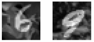
Figure 1: Superimposed images.

The dPCA Alg. 1 was performed on $\{\accentset{\circ}{\mathbf{x}}_{i}\}$ and $\{\accentset{\circ}{\mathbf{y}}_{j}\}$ with $d=2$. PCA was implemented on $\{\accentset{\circ}{\mathbf{x}}_{i}\}$ only. The first two PCs and dPCs are presented in the left and right panels of Fig. 2, respectively. Clearly, dPCA reveals the discriminative information of the target data describing digits $6$ and $9$ relative to the background data, enabling successful discovery of the digit $6$ and $9$ subgroups. On the contrary, PCA captures only the patterns that correspond to the generic background rather than those associated with the digits $6$ and $9$. To further assess the performance of dPCA and PCA, K-means is carried out using the resulting low-dimensional representations of the target data. The clustering performance is evaluated in terms of two metrics: clustering error and scatter ratio. The clustering error is defined as the ratio of the number of incorrectly clustered data vectors over $m$. Scatter ratio verifying cluster separation is defined as $S_{t}/\sum_{i=1}^{2}S_{i}$, where $S_{t}$ and $\{S_{i}\}_{i=1}^{2}$ denote the total scatter value and the within cluster scatter values, given by $S_{t}:=\sum_{j=1}^{2,000}\|\hat{\mathbf{U}}^{\top}\mathbf{x}_{j}\|_{2}^{2}$ and $\{S_{i}:=\sum_{j\in\mathcal{C}_{i}}\|\hat{\mathbf{U}}^{\top}\mathbf{x}_{j}-\hat{\mathbf{U}}^{\top}\sum_{k\in{\mathcal{C}}_{i}}\mathbf{x}_{k}\|_{2}^{2}\}_{i=1}^{2}$, respectively, with $\mathcal{C}_{i}$ representing the set of data vectors belonging to cluster $i$. Table I reports the clustering errors and scatter ratios of dPCA and PCA under different $d$ values. Clearly, dPCA exhibits lower clustering error and higher scatter ratio.

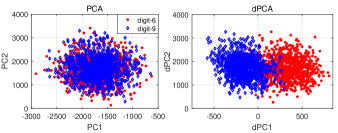
Figure 2: dPCA versus PCA on semi-synthetic images.

TABLE I: Performance comparison between dPCA and PCA.

$d$	Clustering error		Scatter ratio
	dPCA	PCA	dPCA	PCA
1	0.1660	0.4900	2.0368	1.0247
2	0.1650	0.4905	1.8233	1.0209
3	0.1660	0.4895	1.6719	1.1327
4	0.1685	0.4885	1.4557	1.1190
5	0.1660	0.4890	1.4182	1.1085
10	0.1680	0.4885	1.2696	1.0865
50	0.1700	0.4880	1.0730	1.0568
100	0.1655	0.4905	1.0411	1.0508

Real protein expression data [18] were also used to evaluate the ability of dPCA to discover subgroups in real-world conditions. Target data $\{\accentset{\circ}{\mathbf{x}}_{i}\in\mathbb{R}^{77}\}_{i=1}^{267}$ contained $267$ data vectors, each collecting $77$ protein expression measurements of a mouse having Down Syndrome disease [18]. In particular, the first $135$ data points $\{\accentset{\circ}{\mathbf{x}}_{i}\}_{i=1}^{135}$ recorded protein expression measurements of $135$ mice with drug-memantine treatment, while the remaining $\{\accentset{\circ}{\mathbf{x}}_{i}\}_{i=136}^{267}$ collected measurements of $134$ mice without such treatment. Background data $\{\accentset{\circ}{\mathbf{y}}_{j}\in\mathbb{R}^{77}\}_{j=1}^{135}$ on the other hand, comprised such measurements from $135$ healthy mice, which likely exhibited similar natural variations (due to e.g., age and sex) as the target mice, but without the differences that result from the Down Syndrome disease.

When performing cPCA on $\{\accentset{\circ}{\mathbf{x}}_{i}\}$ and $\{\accentset{\circ}{\mathbf{y}}_{j}\}$, four $\alpha$’s were selected from $15$ logarithmically-spaced values between $10^{-3}$ and $10^{3}$ via the spectral clustering method presented in [2].

Experimental results are reported in Fig. 3 with red circles and black diamonds representing sick mice with and without treatment, respectively. Evidently, when PCA is applied, the low-dimensional representations of the protein measurements from mice with and without treatment are distributed similarly. In contrast, the low-dimensional representations cluster two groups of mice successfully when dPCA is employed. At the price of runtime (about $15$ times more than dPCA), cPCA with well tuned parameters ($\alpha=3.5938$ and $27.8256$) can also separate the two groups.

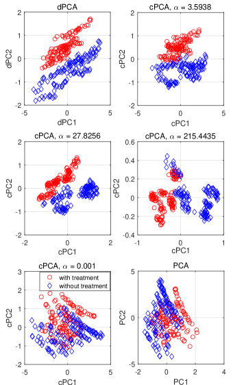
Figure 3: Discovering subgroups in mice protein expression data.

VII-B KdPCA tests

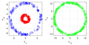
Figure 4: Target data dimension distributions with $x_{i,j}$ representing the $j$-th entry of $\mathbf{x}_{i}$ for $j=1,\,\ldots,\,4$ and $i=1,\,\ldots,\,300$.

In this subsection, our KdPCA is evaluated using synthetic and real data. By adopting the procedure described in [17, p. 546], we generated target data $\{{\mathbf{x}}_{i}:=[x_{i,1}\,x_{i,2}\,x_{i,3}\,x_{i,4}]^{\top}\}_{i=1}^{300}$ and background data $\{{\mathbf{y}}_{j}\in\mathbb{R}^{4}\}_{j=1}^{150}$. In detail, $\{[x_{i,1}\,x_{i,2}]^{\top}\}_{i=1}^{300}$ were sampled uniformly from two circular concentric clusters with corresponding radii $1$ and $6$ shown in the left panel of Fig. 4; and $\{[x_{i,3}\,x_{i,4}]^{\top}\}_{i=1}^{300}$ were uniformly drawn from a circle with radius $10$; see Fig. 4 (right panel) for illustration. The first and second two dimensions of $\{{\mathbf{y}}_{j}\}_{j=1}^{150}$ were uniformly sampled from two concentric circles with corresponding radii of $4$ and $10$. All data points in $\{{\mathbf{x}}_{i}\}$ and $\{{\mathbf{y}}_{j}\}$ were corrupted with additive noise sampled independently from $\mathcal{N}(\mathbf{0},\,0.1\mathbf{I})$. To unveil the specific cluster structure of the target data relative to the background data, Alg. 2 was run with $\epsilon=10^{-3}$ and using the degree-$2$ polynomial kernel $\kappa(\mathbf{z}_{i},\mathbf{z}_{j})=(\mathbf{z}_{i}^{\top}\mathbf{z}_{j})^{2}$. Competing alternatives including PCA, KPCA, cPCA, kernel (K) cPCA [2], and dPCA were also implemented. Further, KPCA and KcPCA shared the kernel function with KdPCA. Three different values of $\alpha$ were automatically chosen for cPCA [2]. The parameter $\alpha$ of KcPCA was set as $1$, $10$, and $100$.

Figure 5 depicts the first two dPCs, cPCs, and PCs of the aforementioned dimensionality reduction algorithms. Clearly, only KdPCA successfully reveals the two unique clusters of $\{{\mathbf{x}}_{i}\}$ relative to $\{{\mathbf{y}}_{j}\}$.

Figure 5: Discovering subgroups in nonlinear synthetic data.

Figure 6: Discovering subgroups in MHealth data.

Figure 7: Distinguishing between waist bends forward and cycling.

Figure 8: Face recognization by performing KdPCA.

KdPCA was tested in realistic settings using the real Mobile (M) Health data [5]. This dataset consists of sensor (e.g., gyroscopes, accelerometers, and EKG) measurements from volunteers conducting a series of physical activities. In the first experiment, $200$ target data $\{{\mathbf{x}}_{i}\in\mathbb{R}^{23}\}_{i=1}^{200}$ were used, each of which recorded $23$ sensor measurements from one volunteer performing two different physical activities, namely laying down and having frontal elevation of arms ($100$ data points correspond to each activity). Sensor measurements from the same volunteer standing still were utilized for the $100$ background data points $\{{\mathbf{y}}_{j}\in\mathbb{R}^{23}\}_{j=1}^{100}$. For KdPCA, KPCA, and KcPCA algorithms, the Gaussian kernel with bandwidth $5$ was used. Three different values for the parameter $\alpha$ in cPCA were automatically selected from a list of $40$ logarithmically-spaced values between $10^{-3}$ and $10^{3}$, whereas $\alpha$ in KcPCA was set to $1$ [2].

The first two dPCs, cPCs, and PCs of KdPCA, dPCA, KcPCA, cPCA, KPCA, and PCA are reported in Fig. 6. It is self-evident that the two activities evolve into two separate clusters in the plots of KdPCA and KcPCA. On the contrary, due to the nonlinear data correlations, the other alternatives fail to distinguish the two activities.

In the second experiment, the target data were formed with sensor measurements of one volunteer executing waist bends forward and cycling. The background data were collected from the same volunteer standing still. The Gaussian kernel with bandwidth $40$ was used for KdPCA and KPCA, while the second-order polynomial kernel $\kappa(\mathbf{z}_{i},\,\mathbf{z}_{j})=(\mathbf{z}_{i}^{\top}\mathbf{z}_{j}+3)^{2}$ was employed for KcPCA. The first two dPCs, cPCs, and PCs of simulated schemes are depicted in Fig. 7. Evidently, KdPCA outperforms its competing alternatives in discovering the two physical activities of the target data.

To test the scalability of our developed schemes, the Extended Yale-B (EYB) face image dataset [25] was adopted to test the clustering performance of KdPCA, KcPCA, and KPCA. EYB database contains frontal face images of $38$ individuals, each having about around $65$ color images of $192\times 168$ ($32,256$) pixels. The color images of three individuals ($60$ images per individual) were converted into grayscale images and vectorized to obtain $180$ vectors of size $32,256\times 1$. The $120$ vectors from two individuals (clusters) comprised the target data, and the remaining $60$ vectors formed the background data. A Gaussian kernel with bandwidth $150$ was used for KdPCA, KcPCA, and KPCA. Figure 8 reports the first two dPCs, cPCs, and PCs of KdPCA, KcPCA (with 4 different values of $\alpha$), and KPCA, with black circles and red stars representing the two different individuals from the target data. K-means is carried out using the resulting $2$-dimensional representations of the target data. The clustering errors of KdPCA, KcPCA with $\lambda=1$, KcPCA with $\lambda=10$, KcPCA with $\lambda=50$, KcPCA with $\lambda=100$, and KPCA are $0.1417$, $0.7$, $0.525$, $0.275$, $0.2833$, and $0.4167$, respectively. Evidently, the face images of the two individuals can be better recognized with KdPCA than with other methods.

VII-C MdPCA tests

The ability of the MdPCA Alg. 3 for discriminative dimensionality reduction is examined here with two background datasets. For simplicity, the involved weights were set to $\omega_{1}=\omega_{2}=0.5$.

In the first experiment, two clusters of $15$-dimensional data points were generated for the target data $\{\accentset{\circ}{\mathbf{x}}_{i}\in\mathbb{R}^{15}\}_{i=1}^{300}$ ($150$ for each). Specifically, the first $5$ dimensions of $\{\accentset{\circ}{\mathbf{x}}_{i}\}_{i=1}^{150}$ and $\{\accentset{\circ}{\mathbf{x}}_{i}\}_{i=151}^{300}$ were sampled from $\mathcal{N}(\mathbf{0},\,\mathbf{I})$ and $\mathcal{N}(8\mathbf{1},\,2\mathbf{I})$, respectively. The second and last $5$ dimensions of $\{\accentset{\circ}{\mathbf{x}}_{i}\}_{i=1}^{300}$ were drawn accordingly from the normal distributions $\mathcal{N}(\mathbf{1},\,10\mathbf{I})$ and $\mathcal{N}(\mathbf{1},\,20\mathbf{I})$. The right top plot of Fig. 9 shows that performing PCA cannot resolve the two clusters. The first, second, and last $5$ dimensions of the first background dataset $\{\accentset{\circ}{\mathbf{y}}_{j}^{1}\in\mathbb{R}^{1}\}_{j=15}^{150}$ were sampled from $\mathcal{N}(\mathbf{1},\,2\mathbf{I})$, $\mathcal{N}(\mathbf{1},\,10\mathbf{I})$, and $\mathcal{N}(\mathbf{1},\,2\mathbf{I})$, respectively, while those of the second background dataset $\{\accentset{\circ}{\mathbf{y}}_{j}^{2}\in\mathbb{R}^{15}\}_{j=1}^{150}$ were drawn from $\mathcal{N}(\mathbf{1},\,2\mathbf{I})$, $\mathcal{N}(\mathbf{1},\,2\mathbf{I})$, and $\mathcal{N}(\mathbf{1},\,20\mathbf{I})$. The two plots at the bottom of Fig. 9 depict the first two dPCs of dPCA implemented with a single background dataset. Evidently, MdPCA can discover the two clusters in the target data by leveraging the two background datasets.

Figure 9: Clustering structure by MdPCA using synthetic data.

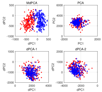
Figure 10: Clustering structure by MdPCA using semi-synthetic data.

In the second experiment, the target data $\{\accentset{\circ}{\mathbf{x}}_{i}\in\mathbb{R}^{784}\}_{i=1}^{400}$ were obtained using $400$ handwritten digits $6$ and $9$ ($200$ for each) of size $28\times 28$ from the MNIST dataset superimposed with $400$ resized ‘girl’ images from the CIFAR-100 dataset [23]. The first $392$ dimensions of the first background dataset $\{\accentset{\circ}{\mathbf{y}}_{j}^{1}\in\mathbb{R}^{784}\}_{j=1}^{200}$ and the last $392$ dimensions of the other background dataset $\{\accentset{\circ}{\mathbf{y}}_{j}^{2}\in\mathbb{R}^{784}\}_{j=1}^{200}$ correspond to the first and last $392$ features of $200$ cropped girl images, respectively. The remaining dimensions of both background datasets were set zero. Figure 10 presents the obtained (d)PCs of MdPCA, dPCA, and PCA, with red stars and black diamonds depicting digits $6$ and $9$, respectively. PCA and dPCA based on a single background dataset (the bottom two plots in Fig. 10) reveal that the two clusters of data follow a similar distribution in the space spanned by the first two PCs. The separation between the two clusters becomes clear when the MdPCA is employed.

VII-D KMdPCA tests

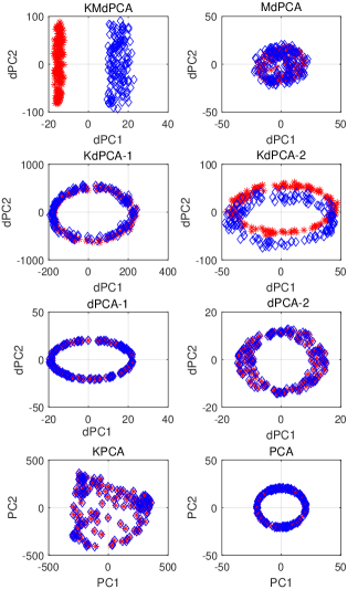
Figure 11: The first two dPCs obtained by Alg. 4.

Algorithm 4 with $\epsilon=10^{-4}$ is examined for dimensionality reduction using simulated data and compared against MdPCA, KdPCA, dPCA, and PCA. The first two dimensions of the target data $\{\mathbf{x}_{i}\in\mathbb{R}^{6}\}_{i=1}^{150}$ and $\{\mathbf{x}_{i}\}_{i=151}^{300}$ were generated from two circular concentric clusters with respective radii of $1$ and $6$. The remaining four dimensions of the target data $\{\mathbf{x}_{i}\}_{i=1}^{300}$ were sampled from two concentric circles with radii of $20$ and $12$, respectively. Data $\{\mathbf{x}_{i}\}_{i=1}^{150}$ and $\{\mathbf{x}_{i}\}_{i=151}^{300}$ corresponded to two different clusters. The first, second, and last two dimensions of one background dataset $\{\mathbf{y}_{j}^{1}\in\mathbb{R}^{6}\}_{j=1}^{150}$ were sampled from three concentric circles with corresponding radii of $3$, $3$, and $12$. Similarly, three concentric circles with radii $3$, $20$, and $3$ were used for generating the other background dataset $\{\mathbf{y}_{j}^{2}\in\mathbb{R}^{6}\}_{j=1}^{150}$. Each datum in $\{\mathbf{x}_{i}\}$, $\{\mathbf{y}_{j}^{1}\}$, and $\{\mathbf{y}_{j}^{2}\}$ was corrupted by additive noise $\mathcal{N}(\mathbf{0},\,0.1\mathbf{I})$. When running KMdPCA, the degree-$2$ polynomial kernel used in Sec. VII-B was adopted, and weights were set as $\omega_{1}=\omega_{2}=0.5$.

Figure 11 depicts the first two dPCs of KMdPCA, MdPCA, KdPCA and dPCA, as well as the first two PCs of (K)PCA. It is evident that only KMdPCA is able to discover the two clusters in the target data.

VIII Concluding Summary

In diverse practical setups, one is interested in extracting, visualizing, and leveraging the unique low-dimensional features of one dataset relative to a few others. This paper put forward a novel framework, that is termed discriminative (d) PCA, for performing discriminative analytics of multiple datasets. Both linear, kernel, and multi-background models were pursued. In contrast with existing alternatives, dPCA is demonstrated to be optimal under certain assumptions. Furthermore, dPCA is parameter free, and requires only one generalized eigenvalue decomposition. Extensive tests using both synthetic and real data corroborated the efficacy of our proposed approaches relative to relevant prior works.

Several directions open up for future research: i) distributed and privacy-aware (MK)dPCA implementations to cope with large amounts of high-dimensional data; ii) robustifying (MK)dPCA to outliers; and iii) graph-aware (MK)dPCA generalizations exploiting additional priors of the data.

We start by showing that

$$\bm{\Phi}^{\top}(\mathbf{Z})\mathbf{C}_{xx}^{\phi}\bm{\Phi}(\mathbf{Z})\mathbf{a}=\mathbf{K}\mathbf{K}^{x}\mathbf{a}\in\mathbb{R}^{N}.$$ (24)

For notational brevity, let $\bm{\phi}_{i}$, $a_{i}$, and $K_{i,j}$ denote the $i$-th column of $\bm{\Phi}(\mathbf{Z})$, the $i$-th entry of $\mathbf{a}$, and the $(i,\,j)$-th entry of $\mathbf{K}$, respectively. Thus, the $i$-th element of the left-hand-side of (24) can be rewritten as

$$\bm{\phi}_{i}^{\top}\frac{1}{m}\sum_{j=1}^{m}\bm{\phi}_{j}\bm{\phi}_{j}^{\top}\sum_{k=1}^{N}a_{k}\bm{\phi}_{k}=\frac{1}{m}\sum_{k=1}^{N}a_{k}\sum_{j=1}^{m}K_{i,j}K_{j,k}$$

$$=\sum_{k=1}^{N}a_{k}\sum_{j=1}^{m}K_{i,j}K_{j,k}^{x}=\sum_{k=1}^{N}a_{k}\sum_{j=1}^{N}K_{i,j}K_{j,k}^{x}$$

$$=\sum_{k=1}^{N}a_{k}s_{i,k}=\mathbf{s}_{i}^{\top}\mathbf{a}=\mathbf{k}_{i}^{\top}\mathbf{K}^{x}\mathbf{a}$$

where $s_{i,k}\in\mathbb{R}$, $\mathbf{s}_{i}^{\top}\in\mathbb{R}^{1\times N}$, and $\mathbf{k}_{i}^{\top}\in\mathbb{R}^{1\times N}$ correspond to the $(i,\,k)$-th entry of $\mathbf{K}\mathbf{K}^{x}$, the $i$-th row of $\mathbf{K}\mathbf{K}^{x}$, and the $i$-th row of $\mathbf{K}$, respectively. Evidently, $\mathbf{k}_{i}^{\top}\mathbf{K}^{x}\mathbf{a}$ is the $i$-th entry of the right-hand-side in (24), which proves that (24) holds. It follows that the numerators of (14) and (17) are identical.

Similarly, one can verify that

$$\mathbf{a}^{\top}\bm{\Phi}^{\top}(\mathbf{Z})\mathbf{C}_{yy}^{\phi}\bm{\Phi}(\mathbf{Z})\mathbf{a}=\mathbf{a}^{\top}\mathbf{K}\mathbf{K}^{y}\mathbf{a}.$$ (25)

Hence, (14) and (17) are equivalent.

References

- [1] H. Abdi, L. J. Williams, and D. Valentin, “Multiple factor analysis: Principal component analysis for multitable and multiblock data sets,” Wiley Interdisciplinary Reviews: Comput. Stat., vol. 5, no. 2, pp. 149–179, Mar. 2013.
- [2] A. Abid, V. K. Bagaria, M. J. Zhang, and J. Zou, “Contrastive principal component analysis,” arXiv:1709.06716, 2017.
- [3] N. Aronszajn, “Theory of reproducing kernels,” Trans. Amer. Math. Soc., vol. 68, no. 3, pp. 337–404, 1950.
- [4] F. R. Bach, G. R. Lanckriet, and M. I. Jordan, “Multiple kernel learning, conic duality, and the SMO algorithm,” in Proc. of Intl. Conf. on Mach. Learn., New York, USA, Jul. 4-8, 2004.
- [5] O. Banos, C. Villalonga, R. Garcia, A. Saez, M. Damas, J. A. Holgado-Terriza, S. Lee, H. Pomares, and I. Rojas, “Design, implementation and validation of a novel open framework for agile development of mobile health applications,” Biomed. Eng. Online, vol. 14, no. 2, p. S6, Dec. 2015.
- [6] E. Barshan, A. Ghodsi, Z. Azimifar, and M. Z. Jahromi, “Supervised principal component analysis: Visualization, classification and regression on subspaces and submanifolds,” Pattern Recognit., vol. 44, no. 7, pp. 1357–1371, 2011.
- [7] M. Belkin and P. Niyogi, “Laplacian eigenmaps for dimensionality reduction and data representation,” Neural Comput., vol. 15, no. 6, pp. 1373–1396, Jun. 2003.
- [8] J. Chen, G. Wang, and Giannakis, “Nonlinear discriminative dimensionality reduction of multiple datasets,” in Proc. of Asilomar Conf. on Signals, Syst., and Comput., Pacific Grove, CA, USA, Oct. 28-31, 2018.
- [9] ——, “Graph multiview canonical correlation analysis,” IEEE Trans. Signal Process., submitted Nov. 2018.
- [10] J. Chen, G. Wang, Y. Shen, and G. B. Giannakis, “Canonical correlation analysis of datasets with a common source graph,” IEEE Trans. Signal Process., vol. 66, no. 16, pp. 4398–4408, Aug. 2018.
- [11] S. Fidler, D. Skocaj, and A. Leibardus, “Combining reconstructive and discriminative subspace methods for robust classification and regression by subsampling,” IEEE Trans. Pattern Analysis & Machine Intell., vol. 28, no. 3, pp. 337–350, Mar. 2006.
- [12] R. A. Fisher, “The use of multiple measurements in taxonomic problems,” Ann. Eugenics, vol. 7, no. 2, pp. 179–188, Sep. 1936.
- [13] K. Fukunaga, Introduction to Statistical Pattern Recognition. 2nd ed., San Diego, CA, USA: Academic Press, Oct. 2013.
- [14] S. Garte, “The role of ethnicity in cancer susceptibility gene polymorphisms: The example of CYP1A1,” Carcinogenesis, vol. 19, no. 8, pp. 1329–1332, Aug. 1998.
- [15] G. B. Giannakis, Y. Shen, and G. V. Karanikolas, “Topology identification and learning over graphs: Accounting for nonlinearities and dynamics,” Proc. IEEE, vol. 106, no. 5, pp. 787–807, May 2018.
- [16] Y. Guo, S. Li, J. Yang, T. Shu, and L. Wu, “A generalized Foley–Sammon transform based on generalized Fisher discriminant criterion and its application to face recognition,” Pattern Recognit. Lett., vol. 24, no. 1-3, pp. 147–158, Jan. 2003.
- [17] T. Hastie, R. Tibshirani, and J. Friedman, The Elements of Statistical Learning 2nd edition. New York: Springer, 2009.
- [18] C. Higuera, K. J. Gardiner, and K. J. Cios, “Self-organizing feature maps identify proteins critical to learning in a mouse model of down syndrome,” PloS ONE, vol. 10, no. 6, p. e0129126, Jun. 2015.
- [19] H. Hotelling, “Relations between two sets of variates,” Biometrika, vol. 28, no. 3/4, pp. 321–377, Dec. 1936.
- [20] C. Hou, F. Nie, and D. Tao, “Discriminative vanishing component analysis,” in AAAI, Phoenix, Arizona, USA, Fec. 12-17, 2016, pp. 1666–1672.
- [21] A. Jaffe and M. Wax, “Single-site localization via maximum discrimination multipath fingerprinting.” IEEE Trans. Signal Process., vol. 62, no. 7, pp. 1718–1728, April 2014.
- [22] F. R. S. Karl Pearson, “LIII. On lines and planes of closest fit to systems of points in space,” The London, Edinburgh, and Dublin Phil. Mag. and J. of Science, vol. 2, no. 11, pp. 559–572, 1901.
- [23] A. Krizhevsky, “Learning multiple layers of features from tiny images,” in Master’s Thesis, Department of Computer Science, University of Toronto, 2009.
- [24] J. B. Kruskal, “Multidimensional scaling by optimizing goodness of fit to a nonmetric hypothesis,” Psychometrika, vol. 29, no. 1, pp. 1–27, Mar. 1964.
- [25] K. C. Lee, J. Ho, and D. J. Kriegman, “Acquiring linear subspaces for face recognition under variable lighting,” IEEE Trans. Pattern Anal. Mach. Intell., vol. 27, no. 5, pp. 684–698, May 2005.
- [26] S. Mika, G. Ratsch, J. Weston, B. Scholkopf, and K.-R. Mullers, “Fisher discriminant analysis with kernels,” in Neural Net. Signal Process. IX: Proc. IEEE Signal Process. Society Workshop, Madison, WI, USA, Aug. 25, 1999, pp. 41–48.
- [27] A. Y. Ng, M. I. Jordan, and Y. Weiss, “On spectral clustering: Analysis and an algorithm,” in Adv. in Neural Inf. Process. Syst., Vancouver, British Columbia, Canada, Dec. 3-8, 2001, pp. 849–856.
- [28] S. T. Roweis and L. K. Saul, “Nonlinear dimensionality reduction by locally linear embedding,” Science, vol. 290, no. 5500, pp. 2323–2326, Dec. 2000.
- [29] Y. Saad, Iterative Methods for Sparse Linear Systems. 2nd ed., Philadelphia, PA, USA: SIAM, 2003.
- [30] B. Scholkopf, A. Smola, and K. B. Muller, Kernel Principal Component Analysis. Berlin, Heidelberg: Springer, 1997, pp. 583–588.
- [31] N. Shahid, N. Perraudin, V. Kalofolias, G. Puy, and P. Vandergheynst, “Fast robust PCA on graphs,” IEEE J. Sel. Topics Signal Process., vol. 10, no. 4, pp. 740–756, Feb. 2016.
- [32] J. Shawe-Taylor and N. Cristianini, Kernel Methods for Pattern Analysis. Cambridge university press, Jun. 2004.
- [33] J. B. Souza Filho and P. S. Diniz, “A fixed-point online kernel principal component extraction algorithm,” IEEE Trans. Signal Process., vol. 65, no. 23, pp. 6244–6259, Dec. 2017.
- [34] J. B. Tenenbaum, V. De Silva, and J. C. Langford, “A global geometric framework for nonlinear dimensionality reduction,” Science, vol. 290, no. 5500, pp. 2319–2323, Dec. 2000.
- [35] N. Tsagkarakis, P. P. Markopoulos, G. Sklivanitis, and D. A. Pados, “L1-norm principal component analysis of complex data,” IEEE Trans. Signal Process., vol. 66, no. 12, pp. 3256–3267, Mar. 2018.
- [36] G. Wang, J. Chen, and G. B. Giannakis, “DPCA: Dimensionality reduction for discriminative analytics of multiple large-scale datasets,” in Proc. of Intl. Conf. on Acoustics, Speech, and Signal Process., Calgary, AB, Canada, April 15-20, 2018.
- [37] B. Yang, “Projection approximation subspace tracking,” IEEE Trans. Signal Process., vol. 43, no. 1, pp. 95–107, Jan. 1995.
- [38] L. Zhang, G. Wang, and G. B. Giannakis, “Going beyond linear dependencies to unveil connectivity of meshed grids,” in IEEE Wkshp. on Comput. Adv. Multi-Sensor Adapt. Process., Curacao, Dutch Antilles, Dec. 2017.
- [39] L. Zhang, G. Wang, D. Romero, and G. B. Giannakis, “Randomized block Frank–Wolfe for convergent large-scale learning,” IEEE Trans. Signal Process., vol. 65, no. 24, pp. 6448–6461, Dec. 2017.