Systematic study of relativistic and chemical enhancements of -odd effects in polar diatomic radicals111Parts of this work were created during the master thesis of Konstantin Gaul.
Abstract
Polar diatomic molecules that have, or are expected to have a -ground state are studied systematically with respect to simultaneous violation of parity and time-reversal with numerical methods and analytical models. Enhancements of -violating effects due to an electric dipole moment of the electron (eEDM) and -odd scalar-pseudoscalar nucleon-electron current interactions are analyzed by comparing trends within columns and rows of the periodic table of the elements. For this purpose electronic structure parameters are calculated numerically within a quasi-relativistic zeroth order regular approximation (ZORA) approach in the framework of complex generalized Hartree-Fock (cGHF) or Kohn-Sham (cGKS). Scaling relations known from analytic relativistic atomic structure theory are compared to these numerical results. Based on this analysis, problems of commonly used relativistic enhancement factors are discussed. Furthermore the ratio between both -odd electronic structure parameters mentioned above is analyzed for various groups of the periodic table. From this analysis an analytic measure for the disentanglement of the two -odd electronic structure parameters with multiple experiments in dependence of electronic structure enhancement factors is derived.
I Introduction
Simultaneous violation of space- () and time-parity () in the charged lepton sector is considered to be a strong indicator for physics beyond the standard model of particle physicsGross (1996). Exploiting enhancement effects in bound systems, such as atoms or molecules, low-energy experiments actually provide the best limits on -violation and thus are among the most useful tools to exclude new physical theories and to test the Standard ModelFortson et al. (2003); Khriplovich and Lamoreaux (1997).
Understanding these atomic and molecular enhancement effects in detail is essential for the development of sensitive experiments.
A permanent atomic or molecular electric dipole moment (EDM) that causes a linear Stark shift in the limit of zero external fields would violate .Khriplovich and Lamoreaux (1997) Mainly four sources of a permanent EDM in molecules are considered: permanent electric dipole moments of the nuclei, -odd nucleon-nucleon current interactions, a permanent electric dipole moment of the electron (eEDM) and -odd nucleon-electron current interactions (see e.g. Ginges and Flambaum (2004)). Of these sources the latter two have the most important contribution in paramagnetic systems.Ginges and Flambaum (2004) Furthermore, nucleon-electron interactions are expected to be dominated by scalar-pseudoscalar interactions, that are nuclear spin independent.
Since the formulation of an eEDM interaction Hamiltonian for atoms by Salpeter in the year 1958Salpeter (1958), there have been many studies on eEDM enhancement in atoms and molecules. Sandars worked out analytical relations of atomic eEDM interactions in the 1960s Sandars (1965, 1966, 1968a, 1968b), which where confirmed also by others some time laterIgnatovich (1969); Flambaum (1976). Sandars calculated, that the enhancement of the eEDM in atoms scales with , where is the fine-structure constant and is the nuclear charge number. Enhancements of scalar-pseudoscalar nucleon-electron current interactions in atoms scale as , as wellKhriplovich (1991). Since then, a number of numerical studies was conducted, but most of the previous investigations focused on the description of -odd effects in individual or few molecular candidates.
Some attempts were made to obtain a deeper understanding of enhancement of -odd effects in molecules beyond established -dependent scaling laws. In Ref. Prasannaa et al., 2015, for instance, the influence of the nuclear charge number of the electronegative partner on eEDM enhancements in mercury monohalides was studied. Furthermore effects of the polarization of the molecule by the electronegative partner on the eEDM enhancement are discussed. In Ref. Prasannaa et al., 2015 it was concluded that the nuclear charge of the lighter halogen atom has lower influence on the eEDM enhancement than its electronegativity.
Recently Sunaga et. al. studied large eEDM enhancement effects in hydrides within orbital interaction theory and remarked an influence of the energy difference between the interacting valence orbitals of the electronegative atom and the unoccupied p1/2 orbital of the heavy atomSunaga et al. (2017). Both of the mentioned studies confirmed that large contributions of s- and p-type atomic orbitals in the singly occupied molecular orbital increase -odd effects, as expectedKhriplovich (1991). A similar result was obtained by Ravaine et. al. in 2005Ravaine et al. (2005), who showed that the covalent character of HI+ causes a stronger s-p-mixing and therefore a larger enhancement of the eEDM than in HBr+, which has an ionic bond.
The majority of previous studies on -violating effects in molecules were performed within a four-component (relativistic) framework. Our recently developed two-component (quasi-relativistic) approach for the calculation of -odd effects allows for routine calculations of a large number of molecules on an ab initio level (see Ref. Gaul and Berger, 2017 for details of the method). In our present paper we thus study systematically a wealth of diatomic radicals across the periodic table, which are known to have a -ground state, or for which at least a -ground state can naively be expected from simple chemical bonding concepts. In combination with analytic scaling relations we calculate the -dependent and -independent electronic structure effects in different groups of the periodic table. Furthermore with an analysis of the behavior of isolobal diatomic molecules we gauge in particular the ”chemical” influences on the -odd enhancement, that is new effects that change between different columns of the periodic table.
We provide with our analysis a consistent overview of -odd effects in a large number of diatomic molecules, which serves as a suitable starting point for further research with higher-level electronic structure methods, where needed. By analysing general trends of the ratio between molecular enhancement factors of the electron electric dipole moment and nucleon-electron current interactions, we draw conclusions on possibilities to disentangle them in experiments with polar diatomic radicals that feature a -ground state.
II Theory
II.1 -odd spin-rotational Hamiltonian
We present herein electronic structure calculations for polar diatomic molecules that are expected to have a -ground state. For these systems an effective spin-rotational Hamiltonian can be derived that in particular describes a transition of Hund’s coupling case (c) to case (b)Hund (1927a, b, c). This corresponds to cases, where the rotational constant is much smaller than the spin-doubling constant but much larger than the -doubling constant (for details see Ref. Kozlov and Labzowsky, 1995). The -odd part of this effective spin-rotational Hamiltonian reads (see e.g. Refs. Dmitriev et al., 1992; Kozlov and Labzowsky, 1995)
| (1) |
where is the projection of the reduced total electronic angular momentum on the molecular axis, defined by the unit vector pointing from the heavy to the light nucleus. is the -odd scalar-pseudoscalar nucleon-electron current interaction constant and is the eEDM. The -odd electronic structure parameters are defined by
| (2a) | ||||
| (2b) | ||||
where is the electronic wave function and the molecular -odd Hamiltonians areSalpeter (1958); Khriplovich and Lamoreaux (1997):
| (3) | ||||
| (4) |
Here is the normalized nuclear density distribution of nucleus with charge number , is the position vector of electron , is the internal electrical field, is Fermi’s weak coupling constant, is the imaginary unit and the Dirac matrices in standard notation are defined as ()
| (5) |
with the vector of the Pauli spin matrices . as reported here is obtained according to Stratagem I of Ref. Lindroth et al., 1989 by commuting the unperturbed Dirac-Coulomb Hamiltonian with a modified momentum operator. We will come back to this in Section II.3.
In this work the electronic structure parameters were calculated, using the corresponding quasi-relativistic Hamiltonians within the zeroth order regular approximation (ZORA)Isaev and Berger (2013); Kudashov et al. (2014); Gaul and Berger (2017)
| (6) | ||||
| (7) |
where is the linear momentum operator, is the commutator and the modified ZORA factors are defined as
| (8) | ||||
| (9) |
with the model potential introduced by van Wüllenvan Wüllen (1998), which is used to alleviate the gauge dependence of ZORA. Here is the speed of light in vacuum and is the mass of the electron. The internal electrical field can be approximated as the field of the nucleiLindroth et al. (1989); Gaul and Berger (2017):
| (10) |
with being the elementary charge and the constant being in SI units with the electric constant . Furthermore the total angular momentum projection was calculated explicitly by
| (11) |
where is the reduced orbital angular momentum operator for electron and is the ZORA multi-electron wave function.
II.2 Scaling-relations of -odd properties
Within the relativistic Fermi-Segrè model for electronic wave functionsFermi and Segrè (1933a) the matrix elements of the -odd operators can be obtained analytically for atomic systemsBouchiat and Bouchiat (1974); Khriplovich (1991). The results for the -odd nucleon-electron current interactions can be expressed in terms of a relativistic enhancement factor
| (12) |
where is the gamma function, and are the nuclear charge and mass numbers, respectively, is the nuclear radius, is the Bohr radius and
| (13) |
with the fine structure constant and the total electronic angular momentum quantum number .
In terms of the relativistic enhancement the parameters of the -odd spin-rotational Hamiltonian can now be estimated to behave as (see Ref. Khriplovich, 1991 for and Ref. Flambaum, 1976 and Ref. Sushkov and Flambaum, 1978 for )
| (14) | ||||
| (15) |
where is a constant that depends on the effective electronic structure of the system under study.
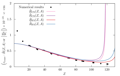
We note in passing, that the relativistic enhancement factor of the eEDM induced permanent atomic EDM is the same as the one for hyperfine interactions published first by Racah in 1931Racah (1931). In relation (15) the label CS indicates that the factor was derived by SandarsSandars (1966) from a method by Casimir. The denominator in relation (15) has two roots: one at and one at . Thus the relativistic enhancement factor causes problems not only for but diverges at for -states (see Figure 1 on page 1). This was also found by Dinh et. al. in a study of hyperfine interactions in super heavy atoms.Dinh et al. (2009) These findings imply that relation (15) is of limited use to estimate for elements with .
An alternative relativistic enhancement factor for hyperfine interactions was found empirically by Fermi and Segrè Fermi and Segrè (1933b, a), who interpolated numerically calculated data by Racah and BreitRacah (1931); Breit (1931):
| (16) |
where the label FS was introduced referring to Fermi and Segrè. has no singularities for , and therefore no severe problems in the description of elements up to are expected. Furthermore, eq. (16) can also be applied to estimate the eEDM enhancement, because the atomic integrals relevant for the hyperfine structure and eEDM enhancement do not differ much within the Fermi-Segrè model and result in the similar enhancement factors differing only by a factor of (see also above and Sandars (1966)):
| (17a) | ||||
| (17b) | ||||
where and are the upper and lower component of the Dirac bi-spinor for a specific orbital angular quantum number , respectively. As , for hydrogen-like atoms, the relativistic enhancement factors are in a first approximation identical up to a factor of . Thus the empirical factor (16) can be employed for our purposes (see also Figure 1 on page 1).
An improved relativistic enhancement factor for the -odd nucleon-electron current interaction parameter was calculated with an analytical atomic model in Dzuba et al. (2011):
| (18) |
with the -dependent function
| (19) |
which results from a polynomial expansion of the atomic wave functions (see appendix of Ref. Dzuba et al., 2011 for details222The explicit numerical factors in were printed partially wrong in Ref. Dzuba et al., 2011, which was mentioned in Ref. Isaev and Berger, 2013.). In Refs. Dzuba et al., 2011; Isaev and Berger, 2013 the eEDM enhancement parameter was estimated from by use of a relativistic enhancement factor for the ratio derived from eqs. (18) and (15):
| (20) |
In combination with summarized conversion factors and constant pre-factors of and
| (21) |
where is Fermi’s constant in atomic units, an estimate for is received from via
| (22) |
When relation (16) is used instead of (15), one obtains an alternative relativistic enhancement factor, which is expected to be more accurate for atoms with a high :
| (23) |
For comparison, instead of the improved relativistic factor for (eq. (18)) relation (14) can be used to receive relativistic enhancement factors:
| (24a) | ||||
| (24b) | ||||
In the following discussion we will show that eq. (16) and (23) indeed agree much better with numerical calculations for than eq. (15) and (20), while there is no appreciable difference for molecules with lighter atoms.
II.3 Neglected many-electron effects in light molecules
The -odd operators shown in II.1 are one-electron operators. Their expectation values scale with the nuclear charge number as . Thus these contributions are dominant in high- molecules. However, in light molecules many-electron effects with lower -dependence stemming from the Hartree–Fock picture or the Breit interaction can have an important contribution to the enhancement factors.
In the following we focus first on additional contributions in the Dirac–Hartree–Fock (DHF) picture that arise from the ZORA transformation. The DHF equation without magnetic fields and with perturbations (4) and (3) reads
| (25) |
where and are the upper and lower components of the Dirac bi-spinor of electron , respectively and is its orbital energy. The nuclear charge density is summarized as and is the potential energy operator appearing on the diagonal, where and are the external and nuclear potential energy operators, respectively. and are the direct parts and , , , are the exchange parts that emerge from the two-electron Coulomb operator in DHF theory. From here on we drop the electron index and the dependencies on the electronic positions for better readability.
Whereas the direct Dirac-Coulomb contributions and are local and appear on the diagonal, the exchange contributions are non-local and non-diagonal
| (26) |
Thus when deriving an approximate relation between and , as when transforming into the ZORA picture, the exchange terms can result in additional contributions to the -odd enhancement.
We start our discussion with the scalar-pseudoscalar nucleon-electron current interaction Hamiltonian. The ZORA Hamiltonian within this perturbation appears as
| (27) |
where is the unperturbed ZORA Hamiltonian in the HF approximation and is the ZORA-factor with the model potential . This results in additional correction terms to (6) stemming from the many-electron mean-field picture (only terms to first order in are shown):
| (28) |
As and the exchange operators , are of , that is of the order of , these corrections are of , whereas the Hamiltonian defined in eq. (3) is of first order in .
We now focus on the eEDM interaction Hamiltonian. The ZORA transformation of the DHF operator using our method from Gaul and Berger (2017) yields:
| (29) |
Thus many-electron mean-field correction terms to (7) are received as
| (30) |
The terms are sorted by their order in the fine structure constant . The first two terms are of and the last term is of and thus is suppressed. The first two terms are suppressed by a factor in comparison to the operator of eq. (7). This is why the correction terms of eq. (28) and (30) have been neglected in the present study even when HF is used. For light elements, however, such terms can be more important, as has been shown e.g. in Ref. Berger (2008)
In a density functional theory (DFT) picture none of the above terms , arises if conventional non-relativistic density functionals are used. Thus we would expect a larger deviation of HF-ZORA from DHF calculations than of Kohn–Sham (KS)-ZORA from Dirac–Kohn–Sham (DKS) calculations. However, if hybrid functionals are used as in our present paper, Fock-exchange is considered explicitly and inclusion of the correction terms mentioned above may become necessary for light elements.
If the above discussed exchange terms become important, terms of comparatively low order which are so far neglected may become important, too. These include the two-electron part of the internal electrical field
| (31) |
However, if an alternative effective one-electron form of operator (4) is used, the two-electron contributions from the electric field can be included implicitly within a mean-field approach.Mårtensson-Pendrill and Öster (1987) Our previous calculationsGaul and Berger (2017) have shown, that these effects are negligible and even for very light molecules as boron monoxide the effects are below 5 % (see Supplemental Material) and are thus not important for the present discussion.
Another term of comparatively low order in is the Breit contribution. The transformed form of the Breit contributions to eEDM enhancement, that corresponds to (4) was derived in Lindroth et al. (1989):
| (32) |
Here we introduced the Dirac matrix . Additional corrections appear from the ZORA transformation, when the Breit interaction, which appears as well on the off-diagonal, is considered (see e.g. Berger (2008)). These Breit interaction corrections appear for as well.
For a more accurate calculation of the eEDM enhancement other magnetic terms of , which were neglected in the deviation in our previous paperGaul and Berger (2017), can play an important role as well and should be considered (see e.g. Lindroth et al. (1989)). For the operator used in this work (eq. (4)) these are
| (33) |
and choosing Coulomb gauge within ZORA they appear as
| (34) |
where with the vector potential . Additional magnetic contributions arise from the ZORA transformation due to the vector potential on the off-diagonal.
Regarding many-body effects of the operator itself, things would become more complicated in a DFT picture, where only one-electron operators are well-defined. Whereas the direct contribution could be calculated analogously to HF, an correction term to the exchange-correlation potential would appear and special exchange-correlation energy functionals would have to be designed. In case of hybrid DFT, additionally Fock exchange contributions would have to be computed. Herein, however, an inclusion of such correction terms is not attempted.
In our present calculations all these many-electron operators are neglected. In principle, this could cause a deviation from comparable four-component calculations which becomes in relative terms more pronounced in light molecules than in high- molecules and are expected to mainly originate from the terms (28) and (30). But these are still expected to be small.
III Computational Details
Quasi-relativistic two-component calculations are performed within ZORA at the level of complex generalized Hartree–Fock (cGHF) or Kohn–Sham (cGKS) with a modified versionBerger and van Wüllen (2005); Berger et al. (2005); Isaev and Berger (2012); Nahrwold and Berger (2009); Gaul and Berger (2017) of the quantum chemistry program package TurbomoleAhlrichs et al. (1989). In order to calculate the -odd properties, the program was extended with the corresponding ZORA Hamiltonians (see Gaul and Berger (2017) for details on the implementation).
For Kohn–Sham (KS)-density functional theory (DFT) calculations the hybrid Becke three parameter exchange functional and Lee, Yang and Parr correlation functional (B3LYP)Stephens et al. (1994); Vosko et al. (1980); Becke (1988); Lee et al. (1988) was employed. For all calculations a basis set of 37 s, 34 p, 14 d and 9 f uncontracted Gaussian functions with the exponential coefficients composed as an even-tempered series as , with for s- and p-function and with for d- and f-functions was used for the electro-positive atom (for details see Supplementary Material). 333For the calculation of row 8 compounds the basis set was augmented with more diffuse functions and a set of g-functions. However, these showed no remarkable influence on -odd properties and thus the results for the same basis set as for the other elements are presented. This basis set has proven successful in calculations of nuclear-spin dependent -violating interactions and -odd effects induced by an eEDM in heavy polar diatomic molecules.Isaev and Berger (2012, 2013, 2014); Gaul and Berger (2017) The N, F and O atoms were represented with a decontracted atomic natural orbital (ANO) basis set of triple- qualityRoos et al. (2004) and for H the s,p-subset of a decontracted correlation-consistent basis of quadruple- qualityDunning (1989) was used.
The ZORA-model potential was employed with additional dampingLiu et al. (2002) as proposed by van Wüllenvan Wüllen (1998). In case of elements of the 8th row, the model potential of Og, the element with highest of all known elements,Oganessian et al. (2006) was renormalized to the respective nuclear charge number.
For the calculations of two-component wave functions and properties a finite nucleus was used, described by a normalized spherical Gaussian nuclear density distribution . The root mean square radius of nucleus was used as suggested by Visscher and Dyall.Visscher and Dyall (1997) The mass numbers were chosen as nearest integer to the standard relative atomic mass, i.e. 11B, 24Mg, 27Al, 40Ca, 45Sc, 48Ti, 65Zn, 70Ga, 88Sr, 90Y, 91Zr, 112Cd, 115In, 137Ba, 139La, 140Ce, 173Yb, 175Lu, 178Hf, 201Hg, 204Tl, 226Ra,227Ac, 232Th, 259No, 260Lr, 261Rf, 284Cn; for E120 (Unbinilium, Ubn, eka-actinium) and E121 (Unbiunium, Ubu, eka-radium) the mass number was calculated by , resulting in 300 and 303, respectively.
The nuclear equilibrium distances were obtained at the levels of GHF-ZORA and GKS-ZORA/B3LYP, respectively. For calculations of energy gradients at the DFT level the nucleus was approximated as a point charge. The distances are given in the results section.
IV Results and Discussion
IV.1 Numerical Calculation of -Violating Properties
In this section the study of quite a number of diatomic molecules with -ground state or for which at least a -ground can be expected, is presented, including group 2 mono-fluorides (Mg–E120)F, group 3 mono-oxides (Sc–E121)O , group 4 mono-nitrides (Ti–Rf)N, group 12 mono-hydrides (Zn–Cn)H, group 13 mono-oxides (B–Tl)O and the mono-nitrides (Ce–Th)N, mono-fluorides (Yb–No)F and mono-oxides (Lu–Lr)O of some f-block groups, respectively.
The numerically calculated values of symmetry violating properties are presented for the listed molecules together with deviations between the methods cGHF and cGKS/B3LYP in Table 1. The calculated equilibrium bond length and numerical values of the reduced total electronic angular momentum projection quantum number are shown as well.
The equilibrium bond lengths and values of determined with GHF and GKS are typically in reasonable agreement. Large deviations in the bond length of about 0.1 are observed for LaO, YbF and group 13 oxides excluding BO, which indicates a more complicated electronic structure. Nearly all values of are approximately equal to . Furthermore in all cases, the reduced orbital angular momentum projection was and thus there appears no significant contamination by -states. Exceptions are CnH and RfN as well as TiN, which show large electron correlation effects (as gauged by the difference GHF-GKS) and seem to have a complicated electronic structure that requires more advanced electronic structure methods for a reliable description. However, even in these cases is valid and there was no significant admixture of -contributions. Especially in case of RfN the methods employed herein are not able to give reliable results, which is indicated by enormous differences between DFT and HF calculations, not only for properties but also for the ordering and pairing of molecular spin-orbitals. The values given for RfN are only included for completeness, but are not to be considered as estimates of the expected effect sizes.
Large deviations between GHF and GKS values of and can be observed for some of the group 13 oxides (esp. AlO and GaO), which indicate that there are electron correlation effects, which can not accurately be described by the present approaches. In these compounds also large spin-polarization effects could be observed. Especially for AlO more sophisticated electronic structure methods should be applied, if more accurate results are desired. Nonetheless for the present discussion of overall trends the description within the cGHF/cGKS scheme appears to suffice.
Generally the agreement between the HF and DFT descriptions is within 20 % to 30 %. Yet, in cases where d-orbitals play an important role, such as group 4 nitrides or group 12 hydrides, additional electron correlation considered via the DFT method has a pronounced impact on the value of the -odd properties. In case of mercury mono-fluoride these effects where already discussed in Ref. Gaul and Berger (2017).
The two parameters and behave analogously with respect to inclusion of additional electron correlation effects when going along the periodic table.
The largest enhancement of -odd effects can be found in compounds of the seventh row of the periodic table, i.e. RaF, AcO, ThN, NoF, LrO, (RfN) and CnH. But also some compounds of the sixth row show enhancement of the similar of magnitude, namely HfN, HgH, TlO, YbF and LuO. It shall be noted, that even the exotic molecule CnH may be a candidate for future experiments, since ongoing research aims to achieve very long lived isotopes for the super heavy element Cn.Oganessian et al. (1999); Oganessian (2011); Utyonkov et al. (2018)
The investigation of -violation in group 13 oxides shows, that especially TlO caused problems for the methods employed herein, as mentioned above. As comparatively large enhancement effects were calculated for TlO, a study of this molecule with more sophisticated electronic structure methods could be interesting in order to obtain an accurate description of its electronic structure. Little is known about TlO from experimental side, however, so that significant further research would be necessary to take advantage of such enhancement effects.
IV.2 Estimation of -Violating Properties from Atomic Scaling Relations
In order to gain deeper insight into the scaling behavior of the above discussed properties the numerical results can be compared to analytical and empirical atomic models. Using the relations presented in the theory section (eqs. (20),(23)) within the quasi-relativistic GHF/GKS-ZORA approach the parameter is estimated from and compared to the results of the numerical calculations.
Results for estimations of from for both the analytically derived expression by Sandars and the empirical factor found by Fermi and Segrè are shown in Table 2 on page 2, where again the labels FS and CS are used for properties calculated with the corresponding factors and .
Relative deviations of the estimated -odd property from the numerical calculations are typically below 10 % for molecules with . For light molecules of the first (BO) or second row (MgF, AlO) the deviations are much larger. In this region the atomic models do not work well. For these cases with light elements both the analytically derived CS-equation and the empirical FS-relation yield much too low (BO, AlO) or too high (MgF) values of . It has to be pointed out, that the case of BO is somewhat special, since boron is even lighter than oxygen and the ”heavy” atom of this molecule is actually oxygen. By this also the sign of the -odd properties and is reversed and a different behavior than for all other group 13 compounds is expected.
In the region of superheavy elements () the abruptly rising analytically derived relativistic enhancement factor of the eEDM (reaching infinity at ) causes a large overestimation of resulting in deviations of for NoF () and LrO () and 146 % for CnH () between the estimate and the numerical value. Here the empirical factor performs much better and a much lower increase in the deviation from the numerical calculations can be observed. However, even in the case of the empirically obtained relativistic enhancement factor the -odd enhancement in superheavy element compounds is strongly overestimated (deviations ) with these simple atomic models. This may be explained with the influence of the pole at of the used relativistic enhancement factors.
For the two studied compounds with the analytically derived factor is not applicable anymore, which results in deviations far beyond 500 %, whereas the estimates obtained with the empirical factor deviate still less than 100 % from numerical calculations. Nonetheless the influence of the pole at of the relativistic enhancement factors for eEDM induced permanent molecular EDMs and scalar-pseudoscalar nucleon-electron current interactions causes deviations .
IV.3 Ratio of -violating properties
Various -odd parameters contribute to a permanent EDM in a molecule. In order to set limits on more than one parameter, experiments with different sensitivity to the -odd parameters have to be compared. In the following we determine the trends of the ratio of -odd enhancement parameters in the periodic table and how the sensitivity of an experiment to the herein discussed -odd effects described by and is influenced by this.
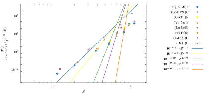
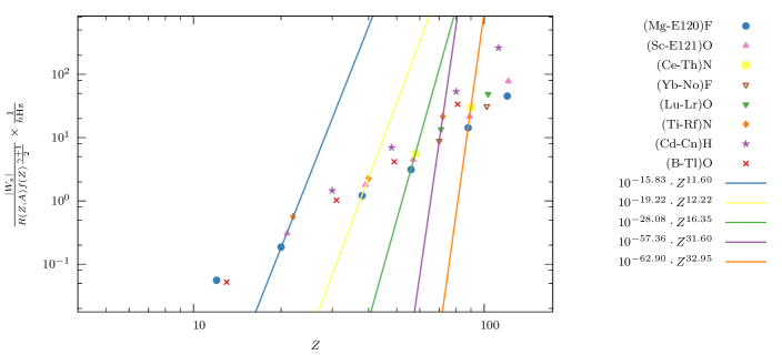
The ratio of the various open-shell diatomic molecules is studied, for which both the analytically derived and the empirically derived relativistic enhancement factors presented in section II are compared. In Figure 2 on page 2 the ratio calculated with the four different relativistic enhancement factors (eqs. (20) to (24b)) is compared to all numerical results for the value of . The empirically derived relativistic enhancement factor for included in eqs. (23) and (24b) is in much better agreement with the numerical results for as was also seen in the last section in the comparison of estimates of with numerical values. Furthermore values calculated with the improved relativistic enhancement factor for (eq. (18)) are in better agreement with numerical values also for .
However, all the ratios derived from the analytical models show a wrong behavior in the region of and in comparison to the numerical results. This causes large deviations for the estimates discussed in the last section.
A logarithmic plot of the numerical results (see Figure 3 on page 3) shows an exponential behavior of the ratio of -odd properties , which can be interpolated by a linear fit model with
| (35) |
In this plot in Figure 3 on page 3 also results of calculations reported by Fleig for the two molecules, HfF+ and ThO, where a -state is of relevance for experiments, are included.Fleig (2017) It can be inferred that the ratio is rather insensitive to the chemical environment of the heavy nucleus, but is essentially determined by the exponential -dependence determined in Figure 3 on page 3.
In order to disentangle the -odd parameters and at least two experiments with molecules 1 and 2 are needed. The measurement model than is a -matrix problem described by the system equations
| (36) |
where is the matrix of sensitivity coefficients. We assume now uncorrelated measurements with standard uncertainties and and the commonly applied case of an ellipsoidal coverage region in the parameter space of and (for details see the Supplementary Material).The ellipse centered at is described by the equation
| (37) |
where for an elliptical region of 95 % probabilityJCGM 102: (2011) and and are the coordinates in the parameter space in direction of and , respectively. Thus the ellipse has an area of
| (38) |
In order two disentangle and in two experiments and set tight limits, assuming equal uncertainties for experiments 1 and 2 the expression
| (39) |
has to become large. The enhancement of the single experiments, which is determined by is strongly dependent on the chemical environment, as will be discussed in the following sections. However, assuming at this point a scaling behavior of as in eq. (15) and eq. (16) for atomic systems, the area of the coverage region is inversely proportional to
| (40) |
Thus, in order to set tight limits on both -odd parameters, experiments with molecules that have a high nuclear charge and at the same time differ considerably in the nuclear charge of the electropositive atom are required. For example when assuming equal uncertainties , a comparison of experiments with YbF and RaF or ThO would provide tighter bounds than a comparison of a BaF experiment with a ThO experiment but also than a comparison of experiments with RaF and ThO. However, the possibilities are limited for paramagnetic molecules because enhancement effects of the individual properties still increase steeply with increasing , which is the dominating effect. Alternatively experiments with diamagnetic atoms and molecules can further tighten bounds on and , as they show different dependencies on the nuclear charge (see e.g. Ref Khriplovich and Lamoreaux, 1997).
This scheme can also be expanded for experiments that aim to set accurate limits on more than the herein discussed parameters. However, for this purpose first the respective enhancement factors have to be calculated for a systematic set of molecules. Furthermore it should be noted that the present picture is not complete because of other sources of permanent EDMs that were not accounted for, namely -odd tensor and pseudoscalar-scalar electron-nucleon current interactions, as well as -odd nuclear dipole moments, which lead to the nuclear Schiff moment and nuclear magnetic quadrupole interactions.
IV.4 Periodic Trends of -Violating Properties
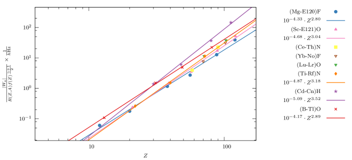
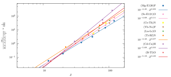
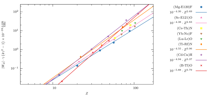
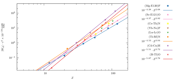
The analytical scaling relations presented in eqs. (18), (15) and (16) can also be used to determine the numerical -scaling within a group of compounds with electropositive atoms of the same column of the periodic table. For this purpose the property is divided by its relativistic enhancement factor and plotted on a double logarithmic scale, as has been done for the nuclear spin-dependent -violating interaction parameter in Isaev and Berger (2012); Borschevsky et al. (2013); Isaev and Berger (2014):
| (41) | ||||
| (42) | ||||
| (43) |
From eqs. (14) and (15) the exponents of can be expected to be approximately three. For both parameters the -scaling is studied herein not only within columns, but also for isolobal diatomics within rows of the periodic table.
The resulting -exponents and factors will be discussed in the following for both, GHF- and GKS-results.
IV.4.1 -Scaling within groups of the periodic table
In the following the scaling within the groups of the periodic table is studied. The graphical representation of the -scaling of and can be found in Figures 4-6. In case of group 13 oxides, boron was not included in the linear fit, because it has a very different character (see discussion above).
Comparing the two different relativistic enhancement factors for eEDM interactions, which were employed in this study, we see for most of the groups of molecules no appreciable differences between the analytically derived and the empirical factor. Yet, in case of group 12 hydrides it is important to use the empirical scaling factor. Cn has a nuclear charge of , which is close to the singularity of the analytically derived factor. This results in a strong overestimation of the relativistic enhancement and thus a strong underestimation of the plotted value, which explains the non-linear trend for group 12 hydrides in Figure 5 on page 5. Furthermore with the analytically derived enhancement factor no meaningful plot that includes the row 8 compounds E120F and E121O is possible. Therefore in the following we will use the results obtained with the empirical enhancement factor for our discussions.
The -scaling parameters and the -independent prefactors are summarized in Table 3 on page 3. It should be noted, that the inclusion of the values of the row 8 compounds into the fit causes no notable changes in the -scaling in case of the eEDM and -odd nucleon-electron current enhancement.
For nearly all parameters the agreement between GHF and GKS calculations is excellent. The only cases, where DFT predicts considerably different behavior, are the group 12 hydride and group 13 oxides. As could be seen in Gaul and Berger (2017) the DFT approach performs much better in the case of group 12 compounds than GHF due to pronounced electron correlation effects and therefore can be taken as more reliable. In the previous sections large electron correlation effects in group 13 compounds, which lead to large differences between GHF an GKS, were already discussed.
The scaling of -odd interactions seems to follow the same laws as that of nuclear spin-dependent -violating interactions studied in Isaev and Berger (2012); Borschevsky et al. (2013). The -scaling increases up to group 12 hydrides, when going along the periods of the periodic table. This maximum effect of -violation enhancement in group 12 compounds is similar to the maximum of relativistic and quantum electrodynamic effects in group 11 compoundsPyykkö and Desclaux (1979); Thierfelder and Schwerdtfeger (2010). At the same time the -independent factor is smallest for these compounds. This damping is, however, only dominant in the region of small , which coincides with the findings in Isaev and Berger (2012) and Borschevsky et al. (2013) for -odd interactions.
In Borschevsky et al. (2013) the large -scaling of group 4 and group 12 compounds compared to group 2 or 3 compounds was attributed mainly to the filling of the d-shells, which causes an increment of the effective nuclear charge because the shielding of the nuclear charge by d-orbitals is less efficient than by s- or p-orbitals. Furthermore therein it was argued that the lower electronegativity of nitrogen compared to oxygen (group 4 shows larger scaling than group 3, although isoelectronic) causes the large effects in group 4 nitrides. A comparison of the molecules with f-block elements next to group 3, that is CeN and ThN, shows a similar behavior as for group 3 or group 2 compounds. Thus the filling of the -shell has a considerable effect on the size of -violating effects as well, which causes group 4 nitrides to be behave differently than group 3 oxides, wheras CeN and ThN are more similar to group 3 oxides.
Relating the -scaling of the fits to the expected -scaling (see eq. (14) and (15)), yields a quantitative -dependent factor for the effects of the molecular electronic structure on -violation. Referring to the GKS result we get an additional scaling factor of for and for for group 2 fluorides, thus there is some damping of -violating effects due to the electronic structure. This can be observed for group 3 oxides regarding eEDM enhancement as well ( for ), but for , in contrast, there is no additional -dependent damping.
A similar damping can be observed for group 13 oxides on the GKS level, whereas GHF predicts a considerable -dependent enhancement instead. The group 4 and 12 compounds show a -dependent enhancement of -odd effects: for and in group 4; for and for in group 12. Thus we see a strong enhancement due to -dependent electronic structure effects in group 12 hydrides, which does not originate from relativistic enhancement factors obtained from atomic considerations.
The -independent electronic structure factors show a behavior inverse to that of and are largest for group 2 fluorides and group 13 oxides in the DFT case, whereas the factors for group 12 hydrides and group 4 nitrides are almost an order of magnitude smaller. Yet, in GHF calculations the -independent effects are on the same order as for group 12 hydrides. Thus, whereas the main enhancement in group 13 oxides is -independent in the DFT description, it is -dependent in the GHF case.
Now we can return to the discussion of disentanglement of and in the two-dimensional parameter space. With the chemical group dependent effective -dependence of the eEDM enhancement factors for paramagnetic molecules, the area covered by two experiments 1 and 2 in the parameter space of and is determined by
| (44) |
Here the factor and the units result from eq. (43), wherein is in units of .
What remains to be analyzed in future works is the detailed influence of molecular orbitals on -violating effects that causes the observed enhancement effects.
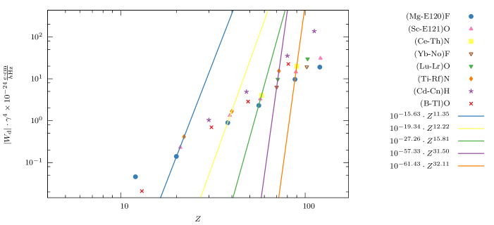
IV.4.2 -Scaling of isolobal molecules
Now we focus on the -scaling for isolobal diatomic molecules within the rows of the periodic table. When discussing eEDM enhancement we concentrate on the results obtained with the empirical relativistic enhancement factor in the following. For comparison, results obtained from the analytically derived relativistic enhancement factor are provided in the Supplemental Material. The corresponding plots can be found in Figure 7 on page 7 for and Figure 8 on page 8 for and the resulting scaling and damping parameters are listed in Table 4 on page 4.
Trends, similar to those reported in Isaev and Berger (2014) for the -odd nucelar spin-dependent interaction can also be observed for the -odd properties. However, we can see a large discrepancy between results obtained from GHF and GKS calculations. Big deviations between the GHF and GKS results in the fourth and fifth row probably stem from electron correlation effects, which lead to a considerable reduction of the -scaling, in group 6 compounds. Fits of the DFT results have large errors that lead to qualitative differences. Especially for row 6 compounds with a filled f-shell (violet line in Figure 7 on page 7 and Figure 8 on page 8) a large fit error can be observed, since HfN does not fold into a linear fit model. The results of GHF fit much better into the trend and show that the scaling behavior of post-f-block compounds of row 6 is approximately similar to that of row 7 compounds without a filled f-shell. Comparing compounds with a filled d-shell (group 12 and 13), we see that the slope becomes negative. This again indicates a maximum of enhancement of -odd effects in group 12 as discussed before.
The investigations show that the chemical environment of the heavy atom can have a much more important effect on the -dependent enhancement than the physical nature of the atom. This can result in effects scaling as for row 7 compounds. Thus a more complex chemical environment may allow for better tuning of the size of -odd enhancement effects. Hence we may speculate that polyatomic molecules might be capable to give larger enhancement effects due to the electronic structure surrounding the heavy atom.
V Conclusion
In this paper we calculated -odd properties due to eEDM and nucleon-electron current interactions in polar open-shell diatomic molecules. We determined periodic trends of -violation by comparison to atomic scaling relations and showed that the trends are very similar to those of nuclear spin-dependent -violating interactions. Furthermore this comparison revealed problems of frequently used scaling relation for eEDM enhancement in the regime of heavy elements with . We showed that an alternative relativistic enhancement factor found empirically by Fermi and Segrè can resolve partially the problems for . Group 12 hydrides and group 4 nitrides were identified to show a very steep -scaling and therefore interesting -dependent electronic structure effects, enhancing -violation in these compounds, were identified. Furthermore, a study of the ratio between -odd properties , showed that electronic structure effects and the chemical environment have a very low influence on the ratio, and the ratio is mainly determined by an exponential dependence on the nuclear charge . Thus for experiments which aim to differentiate between and , the use of molecules with a relatively large difference in nuclear charge would be favorable. The analysis of the scaling of isolobal systems and the study of the ratio showed the limitations of polar diatomic molecules and points to possible advantages in the use of more complex systems, such as polyatomic molecules. The latter will be focus of future research in our lab.
VI Supplemental Material
See the Supplemental Material for details on the used basis sets, further plots of trends derived with the analytical relativistic enhancement factor by Sandars and a comparison of results received from alternative forms of the eEDM interaction Hamiltonian.
Acknowledgements.
Financial support by the State Initiative for the Development of Scientific and Economic Excellence (LOEWE) in the LOEWE-Focus ELCH and computer time provided by the center for scientific computing (CSC) Frankfurt are gratefully acknowledged. T.I. is grateful to RFBR grant N 16-02-01064 for partial support. S.M. gratefully acknowledges support from Fonds der Chemischen Industrie. We thank Yuri Oganessian for inspiring discussions on super heavy elements.References
- Gross (1996) D. J. Gross, Proc. Natl. Acad. Sci. USA 93, 14256 (1996).
- Fortson et al. (2003) N. Fortson, P. Sandars, and S. Barr, Phys. Today 56, 33 (2003).
- Khriplovich and Lamoreaux (1997) I. B. Khriplovich and S. K. Lamoreaux, CP Violation without Strangeness (Springer, Berlin, 1997).
- Ginges and Flambaum (2004) J. S. M. Ginges and V. V. Flambaum, Physics Reports-review Section of Physics Letters 397, 63 (2004).
- Salpeter (1958) E. Salpeter, Phys. Rev. 112, 1642 (1958).
- Sandars (1965) P. Sandars, Phys. Lett. 14, 194 (1965).
- Sandars (1966) P. G. H. Sandars, Phys. Lett. 22, 290 (1966).
- Sandars (1968a) P. G. H. Sandars, J. Phys. B At. Mol. Phys. 1, 511 (1968a).
- Sandars (1968b) P. G. H. Sandars, J. Phys. B At. Mol. Phys. 1, 499 (1968b).
- Ignatovich (1969) V. K. Ignatovich, Sov. J. Exp. Theo. Phys. 29, 1084 (1969).
- Flambaum (1976) V. V. Flambaum, Yad. Fiz. 24, 383 (1976).
- Khriplovich (1991) I. B. Khriplovich, Parity Nonconservation in Atomic Phenomena (Gordon and Breach Science Publ., Philadelphia, 1991).
- Prasannaa et al. (2015) V. S. Prasannaa, A. C. Vutha, M. Abe, and B. P. Das, Phys. Rev. Lett. 114, 183001 (2015), arXiv:1410.5138 .
- Sunaga et al. (2017) A. Sunaga, M. Abe, M. Hada, and B. P. Das, Phys. Rev. A 95, 012502 (2017).
- Ravaine et al. (2005) B. Ravaine, S. G. Porsev, and A. Derevianko, Phys. Rev. Lett. 94, 013001 (2005).
- Gaul and Berger (2017) K. Gaul and R. Berger, J. Chem. Phys. 147, 014109 (2017), arXiv:1703.06838 [physics.chem-ph] .
- Hund (1927a) F. Hund, Z. Phys. 40, 742 (1927a).
- Hund (1927b) F. Hund, Z. Phys. 42, 93 (1927b).
- Hund (1927c) F. Hund, Z. Phys. 43, 805 (1927c).
- Kozlov and Labzowsky (1995) M. G. Kozlov and L. N. Labzowsky, J. Phys. B 28, 1933 (1995).
- Dmitriev et al. (1992) Y. Y. Dmitriev, Y. G. Khait, M. G. Kozlov, L. N. Labzowsky, A. O. Mitrushenkov, A. V. Shtoff, and A. V. Titov, Phys. Lett. A 167, 280 (1992).
- Lindroth et al. (1989) E. Lindroth, B. W. Lynn, and P. G. H. Sandars, J. Phys. B 22, 559 (1989).
- Isaev and Berger (2013) T. A. Isaev and R. Berger, ArXiv e-prints (2013), arXiv:1302.5682 [physics.chem-ph] .
- Kudashov et al. (2014) A. D. Kudashov, A. N. Petrov, L. V. Skripnikov, N. S. Mosyagin, T. A. Isaev, R. Berger, and A. V. Titov, Phys. Rev. A 90, 052513 (2014).
- van Wüllen (1998) C. van Wüllen, J. Chem. Phys. 109, 392 (1998).
- Fermi and Segrè (1933a) E. Fermi and E. Segrè, Z. Phys. 82, 729 (1933a).
- Bouchiat and Bouchiat (1974) M. A. Bouchiat and C. Bouchiat, J. Phys. (Paris) 35, 899 (1974).
- Sushkov and Flambaum (1978) O. P. Sushkov and V. V. Flambaum, Sov. Phys. JETP 48, 608 (1978).
- Racah (1931) G. Racah, Z. Phys. 71, 431 (1931).
- Dinh et al. (2009) T. H. Dinh, V. A. Dzuba, and V. V. Flambaum, Phys. Rev. A 80, 044502 (2009).
- Fermi and Segrè (1933b) E. Fermi and E. Segrè, Mem. Acad. d’Italia 4, 131 (1933b).
- Breit (1931) G. Breit, Phys. Rev. 38, 463 (1931).
- Dzuba et al. (2011) V. A. Dzuba, V. V. Flambaum, and C. Harabati, Phys. Rev. A 84, 052108 (2011).
- Berger (2008) R. Berger, J. Chem. Phys. 129, 154105 (2008).
- Mårtensson-Pendrill and Öster (1987) A. Mårtensson-Pendrill and P. Öster, Phys. Scr. 444, 444 (1987).
- Berger and van Wüllen (2005) R. Berger and C. van Wüllen, J. Chem. Phys. 122, 134316 (2005).
- Berger et al. (2005) R. Berger, N. Langermann, and C. van Wüllen, Phys. Rev. A 71, 042105 (2005).
- Isaev and Berger (2012) T. A. Isaev and R. Berger, Phys. Rev. A 86, 062515 (2012).
- Nahrwold and Berger (2009) S. Nahrwold and R. Berger, J. Chem. Phys. 130, 214101 (2009).
- Ahlrichs et al. (1989) R. Ahlrichs, M. Bär, M. Häser, H. Horn, and C. Kölmel, Chem. Phys. Lett. 162, 165 (1989).
- Stephens et al. (1994) P. J. Stephens, F. J. Devlin, C. F. Chabalowski, and M. J. Frisch, J. Phys. Chem. 98, 11623 (1994).
- Vosko et al. (1980) S. H. Vosko, L. Wilk, and M. Nuisar, Can. J. Phys. 58, 1200 (1980).
- Becke (1988) A. D. Becke, Phys. Rev. A 38, 3098 (1988).
- Lee et al. (1988) C. Lee, W. Yang, and R. G. Parr, Phys. Rev. B 37, 785 (1988).
- Isaev and Berger (2014) T. A. Isaev and R. Berger, J. Mol. Spectrosc. 300, 26 (2014).
- Roos et al. (2004) B. O. Roos, R. Lindh, P. k. Malmqvist, V. Veryazov, and P. O. Widmark, J. Phys. Chem. A 108, 2851 (2004).
- Dunning (1989) T. H. Dunning, Jr., J. Chem. Phys. 90, 1007 (1989).
- Liu et al. (2002) W. Liu, C. van Wüllen, F. Wang, and L. Li, J. Chem. Phys. 116, 3626 (2002).
- Oganessian et al. (2006) Y. T. Oganessian, V. K. Utyonkov, Y. V. Lobanov, F. S. Abdullin, A. N. Polyakov, R. N. Sagaidak, I. V. Shirokovsky, Y. S. Tsyganov, A. A. Voinov, G. G. Gulbekian, S. L. Bogomolov, B. N. Gikal, A. N. Mezentsev, S. Iliev, V. G. Subbotin, A. M. Sukhov, K. Subotic, V. I. Zagrebaev, G. K. Vostokin, M. G. Itkis, K. J. Moody, J. B. Patin, D. A. Shaughnessy, M. A. Stoyer, N. J. Stoyer, P. A. Wilk, J. M. Kenneally, J. H. Landrum, J. F. Wild, and R. W. Lougheed, Phys. Rev. C 74, 044602 (2006).
- Visscher and Dyall (1997) L. Visscher and K. G. Dyall, At. Data Nucl. Data Tables 67, 207 (1997).
- Oganessian et al. (1999) Y. Oganessian, A. Yeremin, G. Gulbekian, S. Bogomolov, V. Chepigin, B. Gikal, V. Gorshkov, M. Itkis, A. Kabachenko, V. Kutner, A. Lavrentev, O. Malyshev, A. Popeko, J. Roháč, R. Sagaidak, S. Hofmann, G. Münzenberg, M. Veselsky, S. Saro, N. Iwasa, and K. Morita, The European Physical Journal A - Hadrons and Nuclei 5, 63 (1999).
- Oganessian (2011) Y. Oganessian, Journal of Physics: Conference Series 312, 082003 (2011).
- Utyonkov et al. (2018) V. K. Utyonkov, N. T. Brewer, Y. T. Oganessian, K. P. Rykaczewski, F. S. Abdullin, S. N. Dmitriev, R. K. Grzywacz, M. G. Itkis, K. Miernik, A. N. Polyakov, J. B. Roberto, R. N. Sagaidak, I. V. Shirokovsky, M. V. Shumeiko, Y. S. Tsyganov, A. A. Voinov, V. G. Subbotin, A. M. Sukhov, A. V. Karpov, A. G. Popeko, A. V. Sabel’nikov, A. I. Svirikhin, G. K. Vostokin, J. H. Hamilton, N. D. Kovrizhnykh, L. Schlattauer, M. A. Stoyer, Z. Gan, W. X. Huang, and L. Ma, Phys. Rev. C 97, 014320 (2018).
- Fleig (2017) T. Fleig, Phys. Rev. A 96, 040502 (2017).
- JCGM 102: (2011) JCGM 102:2011, Evaluation of measurement data – Supplement 2 to the “Guide to the expression of uncertainty in measurement” – Extension to any number of output quantities , Standard (Joint Committee for Guides in Metrology, Paris, FR, 2011).
- Borschevsky et al. (2013) A. Borschevsky, M. Ilias, V. A. Dzuba, V. V. Flambaum, and P. Schwerdtfeger, Phys. Rev. A 88 (2013), 10.1103/PhysRevA.88.022125.
- Pyykkö and Desclaux (1979) P. Pyykkö and J. P. Desclaux, Acc. Chem. Res. 12, 276 (1979).
- Thierfelder and Schwerdtfeger (2010) C. Thierfelder and P. Schwerdtfeger, Phys. Rev. A 82, 062503 (2010).

| Molecule | ** | |||||||||||||
|---|---|---|---|---|---|---|---|---|---|---|---|---|---|---|
| cGHF | cGKS | cGHF | cGKS | cGHF | cGKS | Dev. | cGHF | cGKS | Dev. | |||||
| group 2 fluorides | ||||||||||||||
| MgF | ||||||||||||||
| CaF | ||||||||||||||
| SrF | ||||||||||||||
| BaF | ||||||||||||||
| RaF | ||||||||||||||
| E120F | ||||||||||||||
| group 3 oxides | ||||||||||||||
| ScO | ||||||||||||||
| YO | ||||||||||||||
| LaO | ||||||||||||||
| AcO | ||||||||||||||
| E121O | ||||||||||||||
| group 4 nitrides | ||||||||||||||
| TiN | ||||||||||||||
| ZrN | ||||||||||||||
| HfN | ||||||||||||||
| RfN* | () | () | () | () | () | () | () | () | ||||||
| f-block nitrides | ||||||||||||||
| CeN | ||||||||||||||
| ThN | ||||||||||||||
| f-block fluorides | ||||||||||||||
| YbF | ||||||||||||||
| NoF | ||||||||||||||
| f-block oxides | ||||||||||||||
| LuO | ||||||||||||||
| LrO | ||||||||||||||
| group 12 hydrides | ||||||||||||||
| ZnH | ||||||||||||||
| CdH | ||||||||||||||
| HgH | ||||||||||||||
| CnH | ||||||||||||||
| group 13 oxides | ||||||||||||||
| BO | ||||||||||||||
| AlO | ||||||||||||||
| GaO | ||||||||||||||
| InO | ||||||||||||||
| TlO | ||||||||||||||
-
*
No reliable results could be obtained for RfN.
-
**
The absolute sign of is arbitrary. However, relative to the sign of the effective electric field it is always such that . Exceptions from this (RfN and BO) are discussed in the text.
| cGHF | cGKS | |||||||||
| Molecule | ||||||||||
| group 2 fluorides | ||||||||||
| MgF | ||||||||||
| CaF | ||||||||||
| SrF | ||||||||||
| BaF | ||||||||||
| RaF | ||||||||||
| E120F | ||||||||||
| group 3 oxides | ||||||||||
| ScO | ||||||||||
| YO | ||||||||||
| LaO | ||||||||||
| AcO | ||||||||||
| E121O | ||||||||||
| group 4 nitrides | ||||||||||
| TiN | ||||||||||
| ZrN | ||||||||||
| HfN | ||||||||||
| RfN* | () | () | () | () | ||||||
| f-block nitrides | ||||||||||
| CeN | ||||||||||
| ThN | ||||||||||
| f-block fluorides | ||||||||||
| YbF | ||||||||||
| NoF | ||||||||||
| f-block oxides | ||||||||||
| LuO | ||||||||||
| LrO | ||||||||||
| group 12 hydrides | ||||||||||
| ZnH | ||||||||||
| CdH | ||||||||||
| HgH | ||||||||||
| CnH | ||||||||||
| group 13 oxides | ||||||||||
| BO | ||||||||||
| AlO | ||||||||||
| GaO | ||||||||||
| InO | ||||||||||
| TlO | ||||||||||
-
*
No reliable results could be obtained for RfN.


| Group | |||||||||||
|---|---|---|---|---|---|---|---|---|---|---|---|
| GHF | GKS | GHF | GKS | GHF | GKS | GHF | GKS | ||||
| (Mg-E120)F | p m 0.10 | p m 0.11 | p m 0.16 | p m 0.19 | p m 0.06 | p m 0.08 | p m 0.10 | p m 0.13 | |||
| (Sc-E121)O | p m 0.16 | p m 0.13 | p m 0.2 | p m 0.2 | p m 0.07 | p m 0.10 | p m 0.12 | p m 0.18 | |||
| (Ti-Hf)N | p m 0.4 | p m 0.13 | p m 0.6 | p m 0.2 | p m 0.4 | p m 0.12 | p m 0.6 | p m 0.2 | |||
| (Cd-Cn)H | p m 0.19 | p m 0.13 | p m 0.3 | p m 0.2 | p m 0.11 | p m 0.05 | p m 0.2 | p m 0.08 | |||
| (Al-Tl)O | p m 0.12 | p m 0.05 | p m 0.2 | p m 0.09 | p m 0.12 | p m 0.06 | p m 0.19 | p m 0.08 | |||

| Row | |||||||||||
|---|---|---|---|---|---|---|---|---|---|---|---|
| GHF | GKS | GHF | GKS | GHF | GKS | GHF | GKS | ||||
| 4 (Ca-Ti) | p m 0.8 | p m 1.0 | p m 1.0 | p m 1.4 | p m 0.7 | p m 1.1 | p m 0.9 | p m 1.4 | |||
| 5 (Sr-Zr) | p m 1.6 | p m 2 | p m 2 | p m 3 | p m 1.8 | p m 2 | p m 3 | p m 3 | |||
| 6 (Ba-Ce) | p m 2 | p m 2 | p m 4 | p m 3 | p m 2 | p m 1.8 | p m 4 | p m 3 | |||
| 6 (Yb-Hf) | p m 1.0 | p m 8 | p m 1.8 | p m 15 | p m 0.6 | p m 8 | p m 1.2 | p m 15 | |||
| 7 (Ra-Th) | p m 2 | p m 0.9 | p m 4 | p m 1.8 | p m 2 | p m 1.0 | p m 4 | p m 2 | |||