Mahler Measure and the Vol-Det Conjecture

Abstract.

The Vol-Det Conjecture relates the volume and the determinant of a hyperbolic alternating link in $S^{3}$. We use exact computations of Mahler measures of two-variable polynomials to prove the Vol-Det Conjecture for many infinite families of alternating links.

We conjecture a new lower bound for the Mahler measure of certain two-variable polynomials in terms of volumes of hyperbolic regular ideal bipyramids. Associating each polynomial to a toroidal link using the toroidal dimer model, we show that every polynomial which satisfies this conjecture with a strict inequality gives rise to many infinite families of alternating links satisfying the Vol-Det Conjecture. We prove this new conjecture for six toroidal links by rigorously computing the Mahler measures of their two-variable polynomials.

1. Introduction

The deep connections between the Mahler measure of two-variable polynomials and hyperbolic volume have been investigated by several authors (see, e.g., [5, 6, 9, 26, 29, 24]). The following examples illustrate some of the remarkable relationships that have been discovered: Let $K$ be the figure-eight knot, with $A$-polynomial $A(L,M)$ [20], and let $p(z,w)$ be the characteristic polynomial of the toroidal dimer model on the hexagonal lattice [28]. Let $\mathrm{m}(P)$ denote the logarithmic Mahler measure of a two-variable polynomial $P$, and let ${\rm vol}(K)$ denote the hyperbolic volume of $S^{3}-K$. Then

(1) $${\rm vol}(K)=2\pi\,\mathrm{m}(1+x+y)=\frac{3\sqrt{3}}{2}L(\chi_{-3},2),$$

(2) $${\rm vol}(K)=\pi\,\mathrm{m}(A(L,M))=\pi\,\mathrm{m}(M^{4}+L(1-M^{2}-2M^{4}-M^{6}+M^{8})-L^{2}M^{4}),$$

(3) $${\rm vol}(K)=\frac{2\pi}{5}\,\mathrm{m}(p(z,w))=\frac{2\pi}{5}\,\mathrm{m}\left(6-w-\frac{1}{w}-z-\frac{1}{z}-\frac{z}{w}-\frac{w}{z}\right).$$

Equation (1), a famous result of Smyth [35], was the first instance where Mahler measure, hyperbolic volume and special values of $L$-functions were related. Equation (2), discovered by Boyd [9] and later generalized by Boyd and Rodriguez-Villegas [5, 6], is an example of how Mahler measures of $A$-polynomials, which are invariants of cusped hyperbolic 3-manifolds, are related to sums of hyperbolic volumes of 3-manifolds using regulators on algebraic curves. Equation (3), discovered by Kenyon, arose from his study of the entropy of toroidal dimer models [28].

The Vol-Det Conjecture relates the volume and determinant of a hyperbolic alternating link in $S^{3}$. In this paper, we use exact computations of Mahler measures of two-variable polynomials to prove the Vol-Det Conjecture for many infinite families of alternating links. Specifically, we formulate a conjectured inequality for toroidal links (Conjecture 1 below) that relates hyperbolic geometry, Mahler measure and toroidal dimer models. We then prove that every toroidal link which satisfies Conjecture 1 with a strict inequality gives rise to many infinite families of alternating links satisfying the Vol-Det Conjecture. We prove Conjecture 1 for six toroidal links by explicitly computing the Mahler measures of two variable polynomials using a technique developed by Boyd and Rodriguez-Villegas. In particular, we give the complete proof of equation (3) above. The motivation for Conjecture 1 came from studying the hyperbolic geometry of biperiodic alternating links in [17].

1.1. Main Conjecture

Let $I=(-1,1)$. Let $L$ be a link in the thickened torus $T^{2}\times I$ with an alternating diagram on $T^{2}\times\{0\}$, projected onto the $4$–valent graph $G(L)$. The diagram is cellular if the complementary regions are disks, which are called the faces of $L$ or of $G(L)$. When lifted to the universal cover of $T^{2}\times I$, the link $L$ becomes a biperiodic alternating link $\mathcal{L}$ in $\mathbb{R}^{2}\times I$, such that $L=\mathcal{L}/\Lambda$ for a two-dimensional lattice $\Lambda$ acting by translations of $\mathbb{R}^{2}$. We will refer to $\mathcal{L}$ as a link, even though it has infinitely many components homeomorphic to $\mathbb{R}$ or $S^{1}$. The faces of $\mathcal{L}$ are the complementary regions of its diagram in $\mathbb{R}^{2}$, which are the regions $\mathbb{R}^{2}-G(\mathcal{L})$. The diagram of $L$ on $T^{2}\times\{0\}$ is reduced if four distinct faces meet at every crossing of $G(\mathcal{L})$ in $\mathbb{R}^{2}$. Let $c(L)$ denote the crossing number of the reduced alternating projection of $L$ on $T^{2}\times\{0\}$, which is minimal by [3]. Throughout the paper, link diagrams on $T^{2}\times\{0\}$ will be alternating, reduced and cellular.

Let $B_{n}$ denote the hyperbolic regular ideal bipyramid whose link polygons at the two coning vertices are regular $n$–gons. The hyperbolic volume of $B_{n}$ is given by

$${\rm vol}(B_{n})=n\left(\int_{0}^{2\pi/n}-\log|2\sin(\theta)|d\theta+\int_{0}^{\pi(n-2)/2n}-2\log|2\sin(\theta)|d\theta\right).$$

See [1] for more details and a table of values of ${\rm vol}(B_{n})$. If we let $n=2$, note that ${\rm vol}(B_{2})=0$.

For a face $f$ of a planar or toroidal graph, let $|f|$ denote the degree of the face; i.e., the number of its edges. Let $L$ be an alternating link diagram on the torus as above. Define the bipyramid volume of $L$ as follows:

$${\rm vol}^{\lozenge}(L)=\sum_{f\in\{\text{faces of}\ L\}}{\rm vol}(B_{|f|}).$$

For a biperiodic alternating link $\mathcal{L}$ in $\mathbb{R}^{2}\times I$, the projection graph $G(\mathcal{L})$ in $\mathbb{R}^{2}$ is biperiodic and can be checkerboard colored. The Tait graph $G_{\mathcal{L}}$ is the planar checkerboard graph for which a vertex is assigned to every shaded region and an edge to every crossing of $\mathcal{L}$. Using the other checkerboard coloring yields the dual graph $G_{\mathcal{L}}^{*}$. We form the bipartite overlaid graph $G_{\mathcal{L}}^{b}=G_{\mathcal{L}}\cup G_{\mathcal{L}}^{*}$ determined by the link diagram of $\mathcal{L}$ in $\mathbb{R}^{2}$ as follows: The black vertices of $G_{\mathcal{L}}^{b}$ are the vertices of $G_{\mathcal{L}}$ and of $G_{\mathcal{L}}^{*}$; the white vertices of $G_{\mathcal{L}}^{b}$ are the crossings of $\mathcal{L}$. The edges of $G_{\mathcal{L}}^{b}$ join a black vertex for each face of $\mathcal{L}$ to every white vertex incident to the face. The overlaid graph $G_{\mathcal{L}}^{b}$ is a biperiodic balanced bipartite graph; i.e., the number of black vertices equals the number of white vertices in a fundamental domain. The $\Lambda$–quotient of $G_{\mathcal{L}}^{b}$ is the toroidal graph $G^{b}_{L}$, which is also a balanced bipartite graph. See Figures 3 and 4.

This makes it possible to define the toroidal dimer model on $G^{b}_{L}$. A dimer covering of a graph is a subset of edges that covers all the vertices exactly once, so each vertex is the endpoint of a unique edge. The toroidal dimer model on $G^{b}_{L}$ is a statistical mechanics model of the set of dimer coverings of $G^{b}_{L}$. The characteristic polynomial of the dimer model is defined as $p(z,w)=\det\upkappa(z,w),$ where $\upkappa(z,w)$ is the weighted, signed adjacency matrix with rows indexed by black vertices and columns by white vertices, and matrix entries determined by a certain choice of signs on edges, and a choice of homology basis for the $\Lambda$–action. See Section 2 and [18, 28, 13] for details and examples.

Let $G^{b}_{n}$ be the finite balanced bipartite toroidal graph $G^{b}_{\mathcal{L}}/(n\Lambda)$. Let $Z(G^{b}_{n})$ be the number of dimer coverings of $G^{b}_{n}$. Kenyon, Okounkov and Sheffield [27] gave an explicit expression for the asymptotic growth rate of the toroidal dimer model on $\{G^{b}_{n}\}$:

$$\log Z(G^{b}_{\mathcal{L}}):=\lim_{n\to\infty}\frac{1}{n^{2}}\log Z(G^{b}_{n})=\mathrm{m}(p(z,w)).$$

The number $Z(G^{b}_{\mathcal{L}})$ is called the partition function, and the limit is the entropy of the toroidal dimer model. It is proved in [27] that the Mahler measure of the characteristic polynomial is independent of the choices made to obtain $\upkappa(z,w)$, so the entropy is determined by $G^{b}_{\mathcal{L}}$.

Conjecture 1 (Main Conjecture).

Let $\mathcal{L}$ be any biperiodic alternating link, with toroidally alternating $\Lambda$–quotient link $L$. Let $p(z,w)$ be the characteristic polynomial of the toroidal dimer model on $G_{\mathcal{L}}^{b}$. Then

$${\rm vol}^{\lozenge}(L)\leq 2\pi\,\mathrm{m}(p(z,w)).$$

The link $L$ is often hyperbolic in $T^{2}\times I$; i.e., $(T^{2}\times I)-L$ is a complete finite-volume hyperbolic $3$–manifold [2, 17, 25]. In [17], it was proved that

(4) $${\rm vol}((T^{2}\times I)-L)\leq{\rm vol}^{\lozenge}(L),$$

with equality for semi-regular links. Thus, Conjecture 1 would imply that

(5) $${\rm vol}((T^{2}\times I)-L)\leq{\rm vol}^{\lozenge}(L)\leq 2\pi\,\mathrm{m}(p(z,w)).$$

In this paper, we prove Conjecture 1 for six biperiodic alternating links using rigorous computations for the Mahler measures of the corresponding $p(z,w)$. Our examples include cases for which the expression (5) is sharp, with both equalities, and cases for which both are strict inequalities. We now explain several results at the intersection of geometry, topology and number theory implied by Conjecture 1, which therefore hold in these special cases.

1.2. Volume and determinant.

The determinant of a knot is one of the oldest knot invariants that can be directly computed from a knot diagram. For any knot or link $K$,

$$\det(K)=|\det(M+M^{T})|=|\Delta_{K}(-1)|=|V_{K}(-1)|,$$

where $M$ is any Seifert matrix of $K$, $\Delta_{K}(t)$ is the Alexander polynomial and $V_{K}(t)$ is the Jones polynomial of $K$ (see, e.g., [32]).

Experimental evidence has long suggested a close relationship between the volume and determinant of alternating knots [23, 37]. The following inequality was conjectured in [15], and verified for all alternating knots up to 16 crossings, weaving knots [16] with hundreds of crossings, all 2–bridge links and alternating closed 3–braids [11].

Conjecture 2 (Vol-Det Conjecture [15]).

For any alternating hyperbolic link $K$,

$${\rm vol}(K)<2\pi\log\det(K).$$

It was shown in [15] that the constant $2\pi$ is sharp; i.e., for any $\alpha<2\pi$, there exist alternating links for which ${\rm vol}(K)>\alpha\log\det(K)$.

In [13, 14, 15], biperiodic alternating links were considered as limits of sequences of finite hyperbolic links. In Section 2, we define a natural notion of convergence for a sequence of alternating links to a biperiodic alternating link $\mathcal{L}$, called Følner convergence almost everywhere, denoted by $K_{n}\stackrel{{\scriptstyle\rm{F}}}{{\to}}\mathcal{L}$. It was proved in [13] that for any sequence of alternating links $K_{n}$ that converge to a biperiodic alternating link $\mathcal{L}$ in this sense, the determinant densities of $K_{n}$ converge to the density of the Mahler measure of the characteristic polynomial $p(z,w)$ of the associated toroidal dimer model:

$$K_{n}\stackrel{{\scriptstyle\rm{F}}}{{\to}}\mathcal{L}\quad\Longrightarrow\quad{\lim_{n\to\infty}\frac{\log\det(K_{n})}{c(K_{n})}=\frac{\mathrm{m}(p(z,w))}{c(L)}}.$$

The following theorem implies that whenever Conjecture 1 holds with a strict inequality, we obtain many infinite families of knots that satisfy the Vol-Det Conjecture (Conjecture 2).

Theorem 3.

Let $\mathcal{L}$ be any biperiodic alternating link, with toroidally alternating quotient link $L$. Let $p(z,w)$ be the characteristic polynomial of the associated toroidal dimer model. Let $K_{n}$ be alternating hyperbolic links such that $\displaystyle K_{n}\stackrel{{\scriptstyle\rm{F}}}{{\to}}\mathcal{L}$. If ${\rm vol}^{\lozenge}(L)<2\pi\,\mathrm{m}(p(z,w))$, then ${\rm vol}(K_{n})<2\pi\log\det(K_{n})$ for almost all $n$.

Note that for any $\mathcal{L}$ as in Theorem 3, the infinite families of knots or links satisfying the Vol-Det Conjecture include almost all $K_{n}$ for every sequence $\displaystyle K_{n}\stackrel{{\scriptstyle\rm{F}}}{{\to}}\mathcal{L}$.

1.3. Lower bounds for Mahler measure.

Finding lower bounds for Mahler measure has intrigued mathematicians for more than 80 years. Kronecker’s lemma implies that polynomials in $\mathbb{Z}[z]$ with $\mathrm{m}(p)=0$ are exactly products of cyclotomic polynomials and monomials. Lehmer [31] first asked in 1933 whether there exists $\varepsilon>0$ such that for every $p(z)\in\mathbb{Z}[z]$ with $\mathrm{m}(p)>0$, it follows that $\mathrm{m}(p)>\varepsilon$. Lehmer’s question remains open to this day, although there are several results on specific families of polynomials [10, 34, 4] and general lower bounds that depend on the degree of $p(z)$ [22].

For any multivariable polynomial, Boyd and Lawton [7, 30] showed that its Mahler measure is given by a limit of Mahler measures of single variable polynomials. Therefore, in terms of Lehmer’s question, a lower bound for single variable polynomials would automatically imply a lower bound for multivariable polynomials. Nevertheless, finding multivariable polynomials with low Mahler measure has also attracted interest and speculation [7]. Smyth [36] characterized multivariable polynomials with $\mathrm{m}(p)=0$, generalizing Kronecker’s lemma.

For a two-variable polynomial $p(z,w)$, Smyth’s proof involves the Newton polygon $\Delta(p)$ in $\mathbb{R}^{2}$, which is the convex hull of $\{(m,n)\in\mathbb{Z}^{2}\,|\,\mbox{ the coefficient of }z^{m}w^{n}\mbox{ in }p\mbox{ is non-zero}\}$. For each side $\Delta_{\ell}$ of $\Delta(p)$, one can associate a one-variable polynomial $p_{\ell}$ whose coefficients are those of $p$ corresponding to the points on $\Delta_{\ell}$. Smyth proved that for all $\Delta_{\ell}$,

(6) $$\mathrm{m}(p_{\ell})\leq\mathrm{m}(p).$$

It is interesting to compare the bound in Conjecture 1 with Smyth’s bound (6). For the polynomials we consider in this paper, Conjecture 1 yields a much better bound, and it is actually sharp in two examples, which are discussed in Section 2. Let ${v_{\rm tet}}\approx 1.0149$ be the volume of the regular ideal tetrahedron, ${v_{\rm oct}}\approx 3.6638$ be the volume of the regular ideal octahedron, and $v_{16}\approx 7.8549$ be the volume of the regular ideal bipyramid $B_{8}$. We consider the following polynomials, for which the results are summarized in the table below.

$$\mathcal{P}_{1} = 4+(w+\frac{1}{w}+z+\frac{1}{z})$$

$$\mathcal{P}_{2} = 6-(w+\frac{1}{w}+z+\frac{1}{z}+\frac{w}{z}+\frac{z}{w})$$

$$\mathcal{P}_{3} = -z(w^{2}-4w+1)+w^{2}+4w+1$$

$$\mathcal{P}_{4} = (1+w^{2})(1-z)^{2}-w(6+20z+6z^{2})$$

$$\mathcal{P}_{5} = -w^{2}z^{2}+6w^{2}z+6wz^{2}-w^{2}+28wz-z^{2}+6w+6z-1$$

$p$	$\mathrm{m}(p)$	${\rm vol}^{\lozenge}(L)/2\pi$	maximal $\mathrm{m}(p_{\ell})$
$\mathcal{P}_{1}$	$\frac{2{v_{\rm oct}}}{2\pi}\approx 1.16624361$	$\frac{2{v_{\rm oct}}}{2\pi}\approx 1.16624361$	$\mathrm{m}(z+1)=0$
$\mathcal{P}_{2}$	$\frac{10{v_{\rm tet}}}{2\pi}\approx 1.61532973$	$\frac{10{v_{\rm tet}}}{2\pi}\approx 1.61532973$	$\mathrm{m}(z+1)=0$
$\mathcal{P}_{3}$	$1.65546767$	$\frac{10{v_{\rm tet}}}{2\pi}\approx 1.61532973$	$\mathrm{m}(z^{2}+4z+1)\approx 1.31695789$
$\mathcal{P}_{4}$	$2.79856868$	$\frac{10{v_{\rm tet}}+2{v_{\rm oct}}}{2\pi}\approx 2.78157335$	$\mathrm{m}(z^{2}-6z+1)\approx 1.76274717$
$\mathcal{P}_{5}$	$3.14673710$	$\frac{8{v_{\rm tet}}+{v_{\rm oct}}+v_{16}}{2\pi}\approx 3.12553175$	$\mathrm{m}(z^{2}-6z+1)\approx 1.76274717$

1.4. A typical example for Conjecture 1.

Our proven examples are rather special because the characteristic polynomials that lend themselves to the methods which allow us to compute $\mathrm{m}(p)$ exactly seem to be special. We pause here to present a more typical but only numerically verified example for Conjecture 1.

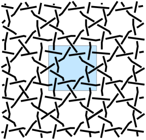
Figure 1. A typical biperiodic alternating link

Figure 1 shows the biperiodic alternating link $\mathcal{L}$, and fundamental domain for its alternating quotient link $L$ in $T^{2}\times I$. The fundamental domain for $L$ has one octagon, four pentagons, one square and eight triangles. Thus, as ${\rm vol}(B_{4})={v_{\rm oct}}$ and ${\rm vol}(B_{3})=2{v_{\rm tet}}$,

$${\rm vol}^{\lozenge}(L)={\rm vol}(B_{8})+4{\rm vol}(B_{5})+{v_{\rm oct}}+16{v_{\rm tet}}\approx 47.704628.$$

Using SnapPy [21] inside Sage to verify the computation rigorously, we verified that

$${\rm vol}((T^{2}\times I)-L)\approx 47.644829.$$

Using the method described in Section 2, we computed the following characteristic polynomial $p(z,w)$, which has genus $8$,

$$p(z,w) = wz^{2}+z^{3}-2wz+104z^{2}-2z^{3}/w+w+510z+510z^{2}/w+z^{3}/w^{2}-2456z/w$$

$$+104z^{2}/w^{2}+510/w+1/z+510z/w^{2}+z^{2}/w^{3}+104/w^{2}-2/(wz)-2z/w^{3}$$

$$+1/w^{3}+1/(w^{2}z)+104.$$

Numerically, $2\pi\,\mathrm{m}(p)\approx 47.9214$, so $L$ satisfies Conjecture 1, and inequality (5) within a range of $0.6\%$,

$${\rm vol}((T^{2}\times I)-L)<{\rm vol}^{\lozenge}(L)<2\pi\,\mathrm{m}(p).$$

1.5. Organization

In Section 2, we recall definitions, properties and examples for the toroidal dimer model, Følner convergence of links, Mahler measure and the Bloch-Wigner dilogarithm. In Section 3, we prove Theorem 3, as well as its corollary, which gives a new bound on how much the volume of a hyperbolic alternating link can change after drilling out an augmented unknot. In Section 4, we prove six special cases of Conjecture 1, and provide numerical evidence to support it.

Acknowledgements

We thank the organizers of the workshop Low-dimensional topology and number theory at MFO (Oberwolfach Research Institute for Mathematics), where this work was started. The first two authors acknowledge support by the Simons Foundation and PSC-CUNY. The third author was partially supported by the Natural Sciences and Engineering Research Council of Canada [Discovery Grant 355412-2013]. We thank the anonymous referee for careful and thoughtful revisions.

2. Background

2.1. Toroidal dimer model

The study of the dimer model is an active research area (see the excellent introductory lecture notes [18, 28]). As mentioned in the Introduction, a dimer covering (or perfect matching) of a graph is a pairing of adjacent vertices. The dimer model on a graph $G$ is a statistical mechanics model of the set of dimer coverings of $G$.

Planar graphs

Let $G$ be a finite balanced bipartite planar graph, with edge weights $\mu_{e}$ for each edge $e$ in $G$. The Kasteleyn signs are a choice of sign for each edge, such that each face of $G$ with $0$ mod $4$ edges has an odd number of negative signs, and each face with $2$ mod $4$ edges has an even number of negative signs. A Kasteleyn matrix $\upkappa$ is a weighted, signed adjacency matrix of $G$, such that rows are indexed by black vertices, and columns by white vertices. The matrix coefficients are $\pm\mu_{e}$, with the sign given by the Kasteleyn sign on $e$. Then, taking the sum over all dimer coverings $M$ of $G$, the partition function $Z(G)$ satisfies (see [18, 28]):

$$Z(G):=\sum_{M}\prod_{e\in M}\mu_{e}=|\det\upkappa|.$$

With $\mu_{e}=1$ for every edge $e$, $Z(G)$ is the number of dimer coverings of $G$. Also see [19] for relations between dimer coverings of planar graphs and knot theory.

Toroidal graphs

Now, let $G$ be a finite balanced bipartite toroidal graph. As in the planar case, we choose Kasteleyn signs on the edges of $G$. We then choose oriented simple closed curves $\gamma_{z}$ and $\gamma_{w}$ on $T^{2}$, transverse to $G$, representing a basis of $H_{1}(T^{2})$. We orient each edge $e$ of $G$ from its black vertex to its white vertex. The weight on $e$ is

$$\mu_{e}=z^{\gamma_{z}\cdot e}w^{\gamma_{w}\cdot e},$$

where $\cdot$ denotes the signed intersection number of $e$ with $\gamma_{z}$ or $\gamma_{w}$. For example, see Figure 2. The Kasteleyn matrix $\upkappa(z,w)$ is the weighted, signed adjacency matrix with rows indexed by black vertices and columns by white vertices, and matrix entries $\pm\mu_{e}$, with the sign given by the Kasteleyn sign on $e$. The characteristic polynomial is defined as

$$p(z,w)=\det\upkappa(z,w).$$

With $\mu_{e}$ as above, the number of dimer coverings of $G$ is given by (see [18, 28]):

$$Z(G)=\frac{1}{2}\ |-p(1,1)+p(-1,1)+p(1,-1)+p(-1,-1)|.$$

Figure 2. (a) Edge weights $\mu_{e}=z^{\gamma_{z}\cdot e}$ to compute $\upkappa(z,w)$. (b) Toroidal bipartite graph $G$ with a choice of Kasteleyn signs.

Biperiodic graphs

Let $G$ be a biperiodic bipartite planar graph, so that translations by a two-dimensional lattice $\Lambda$ act by isomorphisms of $G$. Let $G_{n}$ be the finite balanced bipartite toroidal graph given by the quotient $G/(n\Lambda)$. Kenyon, Okounkov, and Sheffield [27] gave an explicit expression for the growth rate of the toroidal dimer model on $\{G_{n}\}$:

Theorem 4.

[27, Theorem 3.5] Let $G$ be a biperiodic bipartite planar graph. Then

$$\log Z(G):=\lim_{n\to\infty}\frac{1}{n^{2}}\log Z(G_{n})=\mathrm{m}(p(z,w)).$$

Thus, Theorem 4 says that, independent of any choice of Kasteleyn signs and homology basis for the $\Lambda$–action, the growth rate of any toroidal dimer model is given by the Mahler measure of its characteristic polynomial.

In [13], the first two authors defined the following notion of convergence of links in $S^{3}$ to a biperiodic alternating link.

Definition 5 ([13, 15]).

We will say that a sequence of alternating links $K_{n}$ Følner converges almost everywhere to the biperiodic alternating link $\mathcal{L}$, denoted by $K_{n}\stackrel{{\scriptstyle\rm{F}}}{{\to}}\mathcal{L}$, if the respective projection graphs $\{G(K_{n})\}$ and $G(\mathcal{L})$ satisfy the following: There are subgraphs $G_{n}\subset G(K_{n})$ such that

1. $G_{n}\subset G_{n+1}$, and $\bigcup G_{n}=G(\mathcal{L})$,

2. $\lim\limits_{n\to\infty}|\partial G_{n}|/|G_{n}|=0$, where $|\cdot|$ denotes number of vertices, and $\partial G_{n}\subset G(\mathcal{L})$ consists of the vertices of $G_{n}$ that share an edge in $G(\mathcal{L})$ with a vertex not in $G_{n}$,

3. $G_{n}\subset G(\mathcal{L})\cap(n\Lambda)$, where $n\Lambda$ represents $n^{2}$ copies of the $\Lambda$–fundamental domain for the lattice $\Lambda$ such that $L=\mathcal{L}/\Lambda$,

4. $\lim\limits_{n\to\infty}|G_{n}|/c(K_{n})=1$, where $c(K_{n})$ denotes the crossing number of $K_{n}$.

Theorem 6.

[13] Let $\mathcal{L}$ be any biperiodic alternating link, with toroidally alternating quotient link $L$. Let $p(z,w)$ be the characteristic polynomial of the associated toroidal dimer model. Let $K_{n}$ be alternating links such that $\displaystyle K_{n}\stackrel{{\scriptstyle\rm{F}}}{{\to}}\mathcal{L}$. Then

$$\lim_{n\to\infty}\frac{\log\det(K_{n})}{c(K_{n})}=\frac{\mathrm{m}(p(z,w))}{c(L)}.$$

Finally, all of our examples of biperiodic alternating links below satisfy the hypotheses of [17, Theorem 7.5], which implies that the link diagram admits an embedding into $\mathbb{R}^{2}$ for which the faces are cyclic polygons. Such nice geometry allows us to draw the diagrams for their overlaid graphs with vertices at the centers of the corresponding circles.

Example 1: Square weave

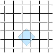
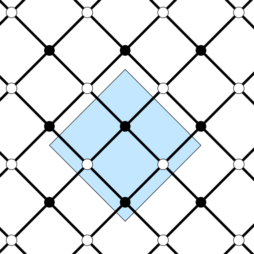
(a)	(b)

Figure 3. (a) Infinite square weave $\mathcal{W}$ and fundamental domain for $W$. (b) Overlaid graph $G_{\mathcal{W}}^{b}$ and fundamental domain for $G_{W}^{b}$.

Figure 3(a) shows the infinite square weave $\mathcal{W}$, with a choice of fundamental domain, giving a toroidally alternating link $W$ with $c(W)=2$. Both of the Tait graphs of $\mathcal{W}$ are the infinite square grid. The overlaid graph $G_{\mathcal{W}}^{b}$ is shown in Figure 3(b), with the fundamental domain for $G_{W}^{b}$, which matches the toroidal graph shown in Figure 2(b).

We can now compute $p(z,w)=\det\upkappa(z,w)$ for $G=G_{W}^{b}$, as described above, and in more detail in [18, 28]. Using Figure 2(b) with the ordering as shown,

(7) $$\upkappa(z,w)=\begin{bmatrix}-1-1/z&1+w\cr 1+1/w&1+z\end{bmatrix},\quad p(z,w)=-\left(4+\frac{1}{w}+w+\frac{1}{z}+z\right).$$

By Theorem 12 below, $\displaystyle 2\pi\,\mathrm{m}(p(z,w))=2\,{v_{\rm oct}}$. By [13, 15], it follows that for $K_{n}\stackrel{{\scriptstyle\rm{F}}}{{\to}}\mathcal{W}$, ${v_{\rm oct}}\approx 3.66386$ is the limit of both determinant densities and volume densities:

$$\lim_{n\to\infty}\frac{2\pi\log\det(K_{n})}{c(K_{n})}=\frac{2\pi\mathrm{m}(p(z,w))}{c(W)}={v_{\rm oct}}=\lim_{n\to\infty}\frac{{\rm vol}(K_{n})}{c(K_{n})}.$$

Example 2: Triaxial link

Figure 4(a) shows part of the biperiodic alternating diagram of the triaxial link $\mathcal{L}$, and the fundamental domain for the toroidally alternating link $L$ with $c(L)=3$. Its projection graph $G(\mathcal{L})$ is the trihexagonal tiling. The Tait graphs of $\mathcal{L}$ are the regular hexagonal and triangular tilings, which form the biperiodic balanced bipartite overlaid graph $G_{\mathcal{L}}^{b}$, shown in Figure 4(b).

We can now compute $p(z,w)=\det\upkappa(z,w)$ for $G=G_{L}^{b}$, as above. Using Figure 4(c), with the homology basis, ordered vertices and a choice of Kasteleyn signs on edges as shown,

(8) $$\upkappa(z,w)=\begin{bmatrix}1&z&w\cr 1&1&1\cr 1/z-1/w&1/w-1&1-1/z\end{bmatrix},\quad p(z,w)=6-\left(\frac{1}{w}+w+\frac{1}{z}+z+\frac{w}{z}+\frac{z}{w}\right).$$

By Theorem 13 below, $\displaystyle 2\pi\,\mathrm{m}(p(z,w))=10{v_{\rm tet}}$, where ${v_{\rm tet}}\approx 1.01494$. By [13], for $K_{n}\stackrel{{\scriptstyle\rm{F}}}{{\to}}\mathcal{L}$,

$$\lim_{n\to\infty}\frac{2\pi\log\det(K_{n})}{c(K_{n})}=\frac{2\pi\mathrm{m}(p(z,w))}{c(L)}=\frac{10{v_{\rm tet}}}{3}.$$

Moreover, by [17],

$$\lim_{n\to\infty}\frac{{\rm vol}(K_{n})}{c(K_{n})}=\frac{{\rm vol}(T^{2}\times I-L)}{c(L)}=\frac{10{v_{\rm tet}}}{3}.$$

For the square weave and the triaxial link, the volume and determinant densities both converge to the volume density of the toroidal link, but we do not know of any other such examples. The strict inequality satisfied by all the other examples in Section 4 seems to be more typical. The first two authors and Purcell compute the exact hyperbolic volume of infinitely many other such biperiodic alternating links in [17].

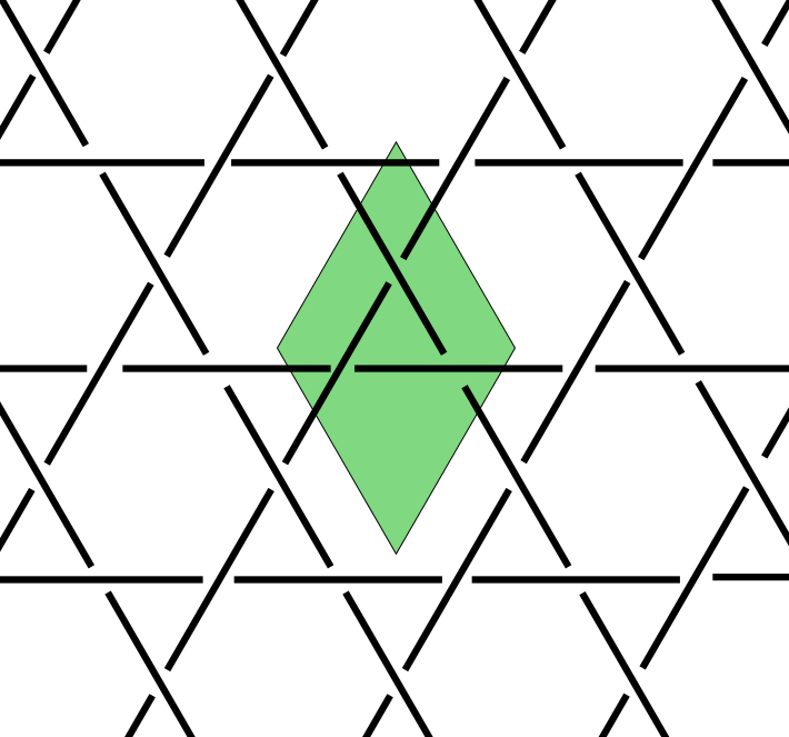
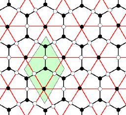
(a)	(b)	(c)

Figure 4. (a) Diagram of biperiodic triaxial link $\mathcal{L}$, and fundamental domain for $L$. (b) Overlaid graph $G_{\mathcal{L}}^{b}$ and fundamental domain for $G_{L}^{b}$. (c) Toroidal graph $G_{L}^{b}$, with a choice of homology basis, ordered vertices and a choice of Kasteleyn signs on edges.

2.2. General Mahler measure theory

Let $P(x_{1},\ldots,x_{n})\in\mathbb{C}[x_{1}^{\pm},\ldots,x_{n}^{\pm}]$ be non-zero, and let $\mathbb{T}^{n}$ denote the unit torus in $\mathbb{C}^{n}$. The logarithmic Mahler measure of $P$ is defined by

$$\mathrm{m}(P)=\frac{1}{(2\pi i)^{n}}\int_{\mathbb{T}^{n}}\log|P(x_{1},\ldots,x_{n})|\;\frac{dx_{1}}{x_{1}}\cdots\frac{dx_{n}}{x_{n}}.$$

We now describe the general method for finding the exact Mahler measure of certain two-variable polynomials, which was developed by Boyd and Rodriguez-Villegas [5, 6]. See also the discussion leading to [38, Theorem 2]. Let $P(x,y)\in\mathbb{C}[x,y]$ be a nonzero polynomial of degree $d$ in $y$. Let $Y$ be the zero locus of $P(x,y)$ and let $X$ be a smooth projective completion of $Y$. If we think of $\mathbb{C}[x,y]=\mathbb{C}[x][y]$, then we may write

$$P(x,y)=P^{*}(x)(y-y_{1}(x))\cdots(y-y_{d}(x)),$$

where $y_{i}(x)$ are algebraic functions of $x$.

By applying Jensen’s formula with respect to the variable $y$, to the integral in the definition of Mahler measure, we obtain

$$\mathrm{m}(P(x,y))-\mathrm{m}(P^{*}(x))= \frac{1}{(2\pi i)^{2}}\int_{\mathbb{T}^{2}}\log|P(x,y)|\frac{dx}{x}\frac{dy}{y}-\mathrm{m}(P^{*})$$

$$= \frac{1}{(2\pi i)^{2}}\int_{\mathbb{T}^{2}}\sum_{j=1}^{d}\log|y-y_{j}(x)|\frac{dx}{x}\frac{dy}{y}$$

$$= \frac{1}{2\pi i}\sum_{j=1}^{d}\int_{|x|=1,|y_{j}(x)|\geq 1}\log|y_{j}(x)|\frac{dx}{x}$$

$$= -\frac{1}{2\pi}\sum_{j=1}^{d}\int_{|x|=1,|y_{j}(x)|\geq 1}\eta(x,y_{j}),$$

where

$$\eta(x,y):=\log|x|d\arg y-\log|y|d\arg x$$

is a closed differential form, and $d\arg z=\mathop{\mathrm{Im}}(dz/z)$. We have that

$$\eta(z,1-z)=dD(z),$$

where $D(z)$ is the Bloch–Wigner dilogarithm given by

(9) $$D(z)=\mathop{\mathrm{Im}}(\mathrm{Li}_{2}(z))+\arg(1-z)\log|z|,$$

and

$$\mathrm{Li}_{2}(z)=-\int_{0}^{z}\frac{\log(1-t)}{t}dt$$

is the classical dilogarithm. While the value of the classical dilogarithm is dependent on the integration path, $D(z)$ is a single-valued continuous function in $\mathbb{P}^{1}(\mathbb{C})$ which is real analytic in $\mathbb{C}-\{0,1\}$.

If we can write

(10) $$x\wedge y_{j}=\sum_{j_{k}}\alpha_{j_{k}}(z_{j_{k}}\wedge(1-z_{j_{k}})),$$

in $\mathbb{C}(X)^{*}\wedge\mathbb{C}(X)^{*}$, then we have

(11) $$\mathrm{m}(P(x,y))-\mathrm{m}(P^{*}(x))=-\frac{1}{2\pi}\sum_{j=1}^{d}\sum_{j_{k}}\alpha_{j_{k}}\left.D(z_{j_{k}})\right|_{\partial\{|x|=1,|y_{j}(x)|\geq 1\}}.$$

It is not clear a priori that equation (10) can be solved for any given $P(x,y)$. Champanerkar [12] showed that for the $A$–polynomial of any $1$–cusped hyperbolic $3$–manifold, (10) can be solved using Thurston’s gluing equations for ideal triangulations. In addition, if the curve attached to our polynomial has genus 0, then it can be parametrized (see [38]). In this case, we will get a solution to (10), possibly with some extra terms of the form $c\wedge z$, where $c$ is a constant, and $z$ is a function. Then, we can still reach a closed formula by integrating $\eta(c,z)$ directly. Note that $\eta(\omega,z)=0$ when $\omega$ is a root of unity. Thus, it is more convenient to work in $(\mathbb{C}(X)^{*}\wedge\mathbb{C}(X)^{*})_{\mathbb{Q}}$, where the subscript indicates tensoring by $\mathbb{Q}$, resulting in the torsion elements removed from consideration.

Lemma 7.

Let $a,b,c,d\in\mathbb{C}$ and $t$ be a variable. If $ad-bc\not=0$, we have, in $(\mathbb{C}(t)^{*}\wedge\mathbb{C}(t)^{*})_{\mathbb{Q}}$,

$$(at+b)\wedge(ct+d)=\frac{act+bc}{ad-bc}\wedge\frac{act+ad}{ad-bc}-(ad-bc)\wedge\frac{act+bc}{act+ad}-c\wedge(ct+d)-(at+b)\wedge a-c\wedge a.$$

Proof.

$$\frac{-(act+bc)}{ad-bc}\wedge\frac{act+ad}{ad-bc}= (-act-bc)\wedge(act+ad)-(-act-bc)\wedge(ad-bc)-(ad-bc)\wedge(act+ad)$$

$$= (-act-bc)\wedge(act+ad)+(ad-bc)\wedge\frac{-(act+bc)}{act+ad}$$

and

$$(-act-bc)\wedge(act+ad)=(-at-b)\wedge(ct+d)+c\wedge(ct+d)+(-at-b)\wedge a+c\wedge a,$$

and we finally use that $(-x)\wedge y=x\wedge y$. ∎

Properties of the Bloch-Wigner dilogarithm

We record here some useful properties of the Bloch–Wigner dilogarithm given by (9). A good reference in the subject is Zagier [39].

Its most fundamental property is the five-term relationship

(12) $$D(x)+D(y)+D(1-xy)+D\left(\frac{1-x}{1-xy}\right)+D\left(\frac{1-y}{1-xy}\right)=0.$$

We will often refer to equation (12) as “the five-term relation generated by $x$ and $y$.” In particular,

(13) $$D\left(\frac{1}{z}\right)=-D(z),{\rm\ and\ }D(1-z)=-D(z).$$

In addition, we have,

(14) $$D(\overline{z})=-D(z).$$

This identity, which is independent of the five-term relation, implies that $\left.D\right|_{\mathbb{R}}=0$.

By taking the five-term relation generated by $z$ and $-z$, we obtain

(15) $$2D(z)+2D(-z)=D(z^{2}).$$

Finally, we record a property that expresses $D(z)$ as a combination of dilogarithms evaluated at complex numbers of norm $1$.

(16) $$D(z)=\frac{1}{2}\left(D\left(\frac{z}{\overline{z}}\right)+D\left(\frac{1-1/z}{1-1/\overline{z}}\right)+D\left(\frac{1/(1-z)}{1/(1-\overline{z})}\right)\right).$$

3. Applications

3.1. Proof of the Vol-Det Conjecture for infinite families of links

In this section, we prove Theorem 3. We will refer to the notation used in Definition 5.

Let $K$ be any hyperbolic alternating link with a reduced alternating diagram, for which the number of bounded $i$–faces of $G(K)$ is $b_{i}$, for all $i>1$. By [1, Theorem 4.1], we get a volume bound for $K$, which is similar to equation (4) for links in $T^{2}\times I$, by excluding the unbounded face of the planar link diagram:

$${\rm vol}(K)\leq{\rm vol}^{\lozenge}(K):=\sum_{f\in\{\begin{subarray}{c}\text{bounded}\\ \text{faces of}\end{subarray}\ K\}}{\rm vol}(B_{|f|})=\sum\nolimits_{i}b_{i}\,{\rm vol}(B_{i}).$$

Theorem 8.

Let $\mathcal{L}$ be any biperiodic alternating link, with toroidally alternating quotient link $L$. Let $K_{n}$ be alternating hyperbolic links such that $\displaystyle K_{n}\stackrel{{\scriptstyle\rm{F}}}{{\to}}\mathcal{L}$. Then

$$\lim_{n\to\infty}\frac{{\rm vol}^{\lozenge}(K_{n})}{c(K_{n})}=\frac{{\rm vol}^{\lozenge}(L)}{c(L)}.$$

Proof.

Let $b_{n,i}$ be the number of bounded $i$–faces of $G(K_{n})$, for $\displaystyle K_{n}\stackrel{{\scriptstyle\rm{F}}}{{\to}}\mathcal{L}$. Then

$$\frac{{\rm vol}^{\lozenge}(K_{n})}{c(K_{n})}:=\frac{\sum_{i}b_{n,i}\,{\rm vol}(B_{i})}{c(K_{n})}.$$

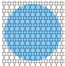
Figure 5. Volume bound for Følner convergence of finite links $K_{n}$ to a biperiodic link $\mathcal{L}$: The part $G_{n}\subset G(\mathcal{L})$ is shown in the disc. As $G_{n}\subset G(K_{n})$, the bipyramid volume density of $K_{n}$ converges to that of $\mathcal{L}$.

Let $G_{n}\subset G(K_{n})$ be as in Definition 5. Since $L=\mathcal{L}/\Lambda$, the projection graph $G(L)$ lifts to a $\Lambda$–fundamental domain graph $\tilde{G}(L)$ for $G(\mathcal{L})$. We consider three mutually exclusive types of bounded faces of $G(K_{n})$ (see Figure 5):

1. Let $b^{\prime}_{n,i}$ be the number of $i$–faces of all copies of $\tilde{G}(L)$ entirely contained in $G_{n}$.

2. Let $b^{\prime\prime}_{n,i}$ be the number of $i$–faces of $G_{n}$ that are not counted in (1).

3. Let $b^{\prime\prime\prime}_{n,i}$ be the number of $i$–faces of $G(K_{n})$ which are not in $G_{n}$.

Note that $b^{\prime}_{n,i}+b^{\prime\prime}_{n,i}$ is the number of $i$–faces of $G_{n}$, and $b^{\prime}_{n,i}+b^{\prime\prime}_{n,i}+b^{\prime\prime\prime}_{n,i}=b_{n,i}$, the number of bounded $i$–faces of $G(K_{n})$.

Now, suppose there are $c_{n}$ copies of $\tilde{G}(L)$ entirely contained in $G_{n}$, so if $b^{L}_{i}$ is the number of $i$–faces of $\tilde{G}(L)$ then $b^{\prime}_{n,i}=c_{n}\,b^{L}_{i}$. Moreover, we can bound the remaining faces of $G_{n}$, which are counted in item (2). Every face of $G_{n}$ counted in $b^{\prime\prime}_{n,i}$ is in a copy of $\tilde{G}(L)$ incident to $\partial G_{n}$, so that $b^{\prime\prime}_{n,i}\leq b^{L}_{i}\,|\partial G_{n}|$. Thus,

$$c_{n}\,|G(L)|\leq|G_{n}|\leq c_{n}\,|G(L)|+|G(L)|\,|\partial G_{n}|.$$

By Definition 5, $\displaystyle\frac{|\partial G_{n}|}{|G_{n}|}\to 0$, so that $\displaystyle\frac{c_{n}\,|G(L)|}{|G_{n}|}\to 1$ as $n\to\infty$. Therefore,

$$\lim_{n\to\infty}\frac{\sum_{i}b^{\prime}_{n,i}\,{\rm vol}(B_{i})}{|G_{n}|}=\lim_{n\to\infty}\frac{\sum_{i}c_{n}\,b^{L}_{i}\,{\rm vol}(B_{i})}{c_{n}\,|G(L)|}=\frac{\sum_{i}b^{L}_{i}\,{\rm vol}(B_{i})}{|G(L)|}=\frac{{\rm vol}^{\lozenge}(L)}{c(L)}.$$

By adding the central axis and stellating each bipyramid, every $B_{i}$ can be decomposed into $i$ tetrahedra (see [17, Figure 15]). Since each tetrahedron contributes at most ${v_{\rm tet}}$ to the hyperbolic volume, ${\rm vol}(B_{i})\leq i\,{v_{\rm tet}}$. Therefore, for every copy of $\tilde{G}(L)$ which is only partially contained in $G_{n}$,

$$\sum\nolimits_{i}b^{\prime\prime}_{n,i}\,{\rm vol}(B_{i})\leq\sum\nolimits_{i}i\,b^{L}_{i}\,{v_{\rm tet}}\,|\partial G_{n}|\leq(4\,|G(L)|){v_{\rm tet}}\,|\partial G_{n}|.$$

For the last inequality, the $i\,b^{L}_{i}$ sum counts with multiplicity the vertices of all faces of $G(L)$, which is $4$–valent, so the sum over all $i$ is bounded by four times the number of its vertices.

For the bounded $i$–faces of $G(K_{n})$ which are not in $G_{n}$,

$$\sum\nolimits_{i}b^{\prime\prime\prime}_{n,i}\,{\rm vol}(B_{i})\leq\sum\nolimits_{i}i\,b^{\prime\prime\prime}_{n,i}\,{v_{\rm tet}}\leq 4{v_{\rm tet}}\,|G(K_{n})-G_{n}|+4{v_{\rm tet}}\,|\partial G_{n}|.$$

The last inequality can be seen as follows: the $i\,b^{\prime\prime\prime}_{n,i}$ sum counts with multiplicity the vertices of all bounded faces of $G(K_{n})$ that are not in $G_{n}$. Since $G(K_{n})$ is 4-valent, the sum over all $i$ is bounded by four times the number of vertices outside $G_{n}$ and vertices of $\partial G_{n}$.

By Definition 5, $\displaystyle\frac{|\partial G_{n}|}{|G_{n}|}\to 0$ and $\displaystyle\frac{|G_{n}|}{c(K_{n})}\to 1$ as $n\to\infty$. Thus, $\displaystyle\frac{|G(K_{n})-G_{n}|}{c(K_{n})}\to 0$, so

$$\lim_{n\to\infty}\frac{{\rm vol}^{\lozenge}(K_{n})}{c(K_{n})} = \lim_{n\to\infty}\frac{\sum_{i}(b^{\prime}_{n,i}+b^{\prime\prime}_{n,i}+b^{\prime\prime\prime}_{n,i})\,{\rm vol}(B_{i})}{c(K_{n})}$$

$$= \lim_{n\to\infty}\frac{\sum_{i}b^{\prime}_{n,i}\,{\rm vol}(B_{i})}{|G_{n}|}+{\rm O}\left(\frac{|\partial G_{n}|}{|G_{n}|}\right){v_{\rm tet}}+{\rm O}\left(\frac{|G(K_{n})-G_{n}|}{c(K_{n})}\right){v_{\rm tet}}$$

$$= \frac{{\rm vol}^{\lozenge}(L)}{c(L)}.$$

∎

Proof of Theorem 3.

Since ${\rm vol}(K)\leq{\rm vol}^{\lozenge}(K)$,

$$\frac{{\rm vol}(K_{n})}{c(K_{n})}\leq\frac{{\rm vol}^{\lozenge}(K_{n})}{c(K_{n})}.$$

Hence, the hypothesis ${\rm vol}^{\lozenge}(L)<2\pi\,\mathrm{m}(p(z,w))$ and Theorem 8 imply that

(17) $$\lim_{n\to\infty}\frac{{\rm vol}(K_{n})}{c(K_{n})}\leq\lim_{n\to\infty}\frac{{\rm vol}^{\lozenge}(K_{n})}{c(K_{n})}=\frac{{\rm vol}^{\lozenge}(L)}{c(L)}<\frac{2\pi\,\mathrm{m}(p(z,w))}{c(L)}.$$

By Theorem 6, $\displaystyle K_{n}\stackrel{{\scriptstyle\rm{F}}}{{\to}}\mathcal{L}$ implies

$$\lim_{n\to\infty}\frac{\log\det(K_{n})}{c(K_{n})}=\frac{\mathrm{m}(p(z,w))}{c(L)}.$$

Therefore,

$$\lim_{n\to\infty}\frac{{\rm vol}(K_{n})}{c(K_{n})}<\lim_{n\to\infty}\frac{2\pi\,\log\det(K_{n})}{c(K_{n})},$$

which proves the claim. ∎

Remark 9.

The proof above fails without the hypothesis ${\rm vol}^{\lozenge}(L)<2\pi\,\mathrm{m}(p(z,w))$, when $\displaystyle\lim_{n\to\infty}\frac{{\rm vol}(K_{n})}{c(K_{n})}=\lim_{n\to\infty}\frac{2\pi\log\det(K_{n})}{c(K_{n})}$. This happens in only two cases that we know of: the square weave $\mathcal{W}$ and the triaxial link $\mathcal{L}$ discussed in Section 4.2. Nevertheless, we checked numerically for weaving knots $\displaystyle K_{n}\stackrel{{\scriptstyle\rm{F}}}{{\to}}\mathcal{W}$ (see [16]) with hundreds of crossings that the Vol-Det Conjecture does hold.

3.2. Bound on volume change under augmentation

In [14], it was shown that the Vol-Det Conjecture implies the following conjecture, which would be a new upper bound for how much the volume can change after drilling out an augmented unknot:

Conjecture 10 ([14]).

For any hyperbolic alternating link $K$ with an augmented unknot $B$ around any two parallel strands of $K$,

$${\rm vol}(K)<{\rm vol}(K\cup B)\leq 2\pi\log\det(K).$$

In this section, we prove Conjecture 10 for infinite families of knots or links that include almost all $K_{n}$ for every sequence $\displaystyle K_{n}\stackrel{{\scriptstyle\rm{F}}}{{\to}}\mathcal{L}$ as in Theorem 3.

Corollary 11.

Let $K_{n}\stackrel{{\scriptstyle\rm{F}}}{{\to}}\mathcal{L}$ be links satisfying the conditions of Theorem 3. Then for almost all $n$,

$${\rm vol}(K_{n})<{\rm vol}(K_{n}\cup B)<2\pi\log\det(K_{n}).$$

Proof.

Since volume increases under Dehn drilling, ${\rm vol}(K_{n})<{\rm vol}(K_{n}\cup B)$. Although we do not know that volume densities of $K_{n}$ converge to that of $\mathcal{L}$ (see [17, Conjecture 6.5]), Theorem 8 implies $\displaystyle\limsup_{n\to\infty}\frac{{\rm vol}(K_{n})}{c(K_{n})}\leq\frac{{\rm vol}^{\lozenge}(L)}{c(L)}$.

Figure 6. Augmented hyperbolic alternating links $K\cup B$ and $K^{m}\cup B$

Let $K\cup B$ be any augmented alternating link, and let $K^{m}$ denote the $m$–periodic alternating link with quotient $K$, formed by taking $m$ copies of a tangle $T$ as in Figure 6. It was shown in [14] that

$$\lim_{m\to\infty}\frac{{\rm vol}(K^{m})}{c(K^{m})}=\frac{{\rm vol}(K\cup B)}{c(K)},\text{\ and \ }\lim_{m\to\infty}\frac{2\pi\log\det(K^{m})}{c(K^{m})}=\frac{2\pi\log\det(K)}{c(K)}.$$

Thus, for all $m$, $\displaystyle\limsup_{n\to\infty}\frac{{\rm vol}(K_{n}^{m})}{c(K_{n}^{m})}\leq\frac{{\rm vol}^{\lozenge}(L)}{c(L)}+\epsilon(m)$, such that $\lim_{m\to\infty}\epsilon(m)=0$. It follows that $\displaystyle\limsup_{m,n\to\infty}\frac{{\rm vol}(K_{n}^{m})}{c(K_{n}^{m})}\leq\frac{{\rm vol}^{\lozenge}(L)}{c(L)}$. Therefore,

$$\frac{{\rm vol}(K_{n}\cup B)}{c(K_{n})}=\lim_{m\to\infty}\frac{{\rm vol}(K_{n}^{m})}{c(K_{n}^{m})}\leq\limsup_{m,n\to\infty}\frac{{\rm vol}(K_{n}^{m})}{c(K_{n}^{m})}\leq\frac{{\rm vol}^{\lozenge}(L)}{c(L)}<\frac{2\pi\log\det(K_{n})}{c(K_{n})}$$

for almost all $n$, where the final inequality follows by inequality (17) and Theorem 6. ∎

4. Proven examples for Conjecture 1

To review notation, recall that ${v_{\rm tet}}$ is the volume of the regular ideal tetrahedron, and ${v_{\rm oct}}$ is the volume of the regular ideal octahedron:

$${v_{\rm tet}}=D\left(e^{i\pi/3}\right)=D\left(\frac{1+\sqrt{3}i}{2}\right)\approx 1.01494,\quad{v_{\rm oct}}=4D\left(e^{i\pi/2}\right)=4D(i)\approx 3.66386.$$

4.1. Square weave

Our first example is the square weave $\mathcal{W}$, as shown in Figure 3, which was discussed in Example 1 of Section 2. Let $W$ be its alternating quotient link in $T^{2}\times I$ as in Section 2. By equation (7),

$$p_{W}(z,w)=-\left(4+w+\frac{1}{w}+z+\frac{1}{z}\right).$$

In [8], Boyd gives the main idea how to prove a formula for the Mahler measure of $p_{W}(z,w)$. Below we provide the missing details, including the dilogarithm evaluation using formula (11).

Theorem 12.

$$2\pi\,\mathrm{m}(p_{W})=8D(i)=2{v_{\rm oct}}.$$

Consequently, ${\rm vol}((T^{2}\times I)-W)={\rm vol}^{\lozenge}(W)=2\pi\,\mathrm{m}(p_{W})$.

Proof.

Consider the factorization due to Boyd [8]:

$$q(z,w)=-p_{W}(z/w,wz)= 4+\left(wz+\frac{1}{wz}+\frac{z}{w}+\frac{w}{z}\right)$$

$$= \frac{1}{wz}(1+iw+iz+wz)(1-iw-iz+wz).$$

Note that $\mathrm{m}(1-iw-iz+wz)=\mathrm{m}(1+iw+iz+wz)$ since one is obtained from the other by $z\to-z$ and $w\to-w$, which does not alter the Mahler measure. Hence $\mathrm{m}(p_{W})=2\mathrm{m}(q_{1})$ where $q_{1}(z,w)=1+iw+iz+wz$.

Let us compute $\mathrm{m}(q_{1})$. Setting $w=e^{i\theta}$ we get

$$|z|=\left|\frac{1+iw}{w+i}\right|=\left|\frac{1+iw}{1-iw}\right|=\left|\frac{1+e^{i(\theta+\pi/2)}}{1-e^{i(\theta+\pi/2)}}\right|=\left|\cot\left(\frac{2\theta+\pi}{4}\right)\right|.$$

Then $|z|\geq 1$ iff $-\pi\leq\theta\leq 0$. Therefore we have to integrate between $w=-1$ and $w=1$. The wedge product can be decomposed as

$$w\wedge z=w\wedge\frac{1+iw}{i+w}=w\wedge\frac{1+iw}{1-iw}=iw\wedge(1+iw)-iw\wedge(1-iw).$$

Applying (11), we evaluate $-\frac{1}{2\pi}(D(-iw)-D(iw))$ on the boundary $w\rvert_{\text{\tiny-1}}^{\text{\tiny 1}}$ to obtain

$$2\pi\mathrm{m}(q_{1})=-D(-i\cdot 1)+D(i\cdot 1)+D(-i\cdot(-1))-D(i\cdot(-1))=4D(i).$$

Thus, we obtain the first claim:

$$2\pi\mathrm{m}(p_{W})=4\pi\mathrm{m}(q_{1})=8D(i)=2{v_{\rm oct}}.$$

By [17, Theorem 3.5],

$${\rm vol}((T^{2}\times I)-W)={\rm vol}^{\lozenge}(W)=2{v_{\rm oct}}.$$

Thus, Conjecture 1 is verified for the square weave $\mathcal{W}$ with an equality. ∎

4.2. Triaxial link

Next, we consider the triaxial link $\mathcal{L}$ as shown in Figure 4, which was discussed in Example 2 of Section 2. Let $L$ be its alternating quotient link in $T^{2}\times I$ as in Section 2. By equation (8),

$$p_{L}(z,w)=6-\left(w+\frac{1}{w}+z+\frac{1}{z}+\frac{w}{z}+\frac{z}{w}\right).$$

In [8], Boyd mentions without giving the proof that the Mahler measure of $p_{L}(z,w)$ can be found by using equation (11). Below we provide the proof.

Theorem 13.

$$2\pi\,\mathrm{m}(p_{L})=10D\left(\frac{1+\sqrt{3}}{2}\right)=10{v_{\rm tet}}.$$

Consequently, ${\rm vol}((T^{2}\times I)-L)={\rm vol}^{\lozenge}(L)=2\pi\,\mathrm{m}(p_{L})$.

Proof.

We can parametrize the curve defined by $p_{L}(z,w)=0$ by using standard algorithms (see, e.g., [33, Chapter 4]). We obtain

$$z=-\frac{(2t-1)(t-1)}{t+1},\qquad w=-\frac{(t-2)(t-1)}{t(t+1)}.$$

Setting $w=e^{i\theta}$ we write

$$e^{i\theta}=-\frac{(t-2)(t-1)}{t(t+1)}\implies(e^{i\theta}+1)t^{2}+(e^{i\theta}-3)t+2=0.$$

Since $\displaystyle{|z|=\left|\frac{(2t-1)(t-1)}{t+1}\right|}$ and we have to integrate for $|z|\geq 1$, it can be seen that the integration domain is given by $\theta\in(0,2\pi)$ and that this corresponds to a path for $t$ that has boundary points in $t=\frac{1-\sqrt{3}i}{2}$ and $t=\frac{1+\sqrt{3}i}{2}$.

We also have

$$w\wedge z= \frac{(t-2)(t-1)}{t(t+1)}\wedge\frac{(2t-1)(t-1)}{t+1}$$

$$= (t-2)\wedge(2t-1)+(t-2)\wedge(t-1)-(t-2)\wedge(t+1)+(t-1)\wedge(2t-1)$$

$$-t\wedge(2t-1)-t\wedge(t-1)+t\wedge(t+1)-(t+1)\wedge(2t-1).$$

Applying Lemma 7 (and ignoring the terms of the form $(\pm 1)\wedge x$ and $x\wedge(\pm 1)$) we can express every term as a combination of terms of the form $\alpha\wedge(1-\alpha)$ as follows:

$$(t-2)\wedge(2t-1)= \frac{4-2t}{3}\wedge\frac{2t-1}{3}-3\wedge\frac{4-2t}{2t-1}-2\wedge(2t-1)$$

$$(t-2)\wedge(t-1)= (2-t)\wedge(t-1)$$

$$(t-2)\wedge(t+1)= \frac{2-t}{3}\wedge\frac{t+1}{3}-3\wedge\frac{2-t}{t+1}$$

$$(t-1)\wedge(2t-1)= (2-2t)\wedge(2t-1)-2\wedge(2t-1)$$

$$t\wedge(2t-1)= (2t)\wedge(1-2t)-2\wedge(2t-1)$$

$$t\wedge(t-1)= t\wedge(1-t)$$

$$t\wedge(t+1)= (-t)\wedge(t+1)$$

$$(t+1)\wedge(2t-1)= \frac{2t+2}{3}\wedge\frac{1-2t}{3}-3\wedge\frac{2t+2}{2t-1}-2\wedge(2t-1).$$

Thus, we obtain

$$w\wedge z= \frac{4-2t}{3}\wedge\frac{2t-1}{3}+(2-t)\wedge(t-1)-\frac{2-t}{3}\wedge\frac{t+1}{3}+(2-2t)\wedge(2t-1)$$

$$-(2t)\wedge(1-2t)-t\wedge(1-t)+(-t)\wedge(t+1)-\frac{2t+2}{3}\wedge\frac{1-2t}{3}.$$

Using equation (11), this integrates to

$$-D\left(\frac{2t-1}{3}\right)-D(t-1)+D\left(\frac{t+1}{3}\right)-D(2t-1)-D(2t)-D(t)+D(-t)-D\left(\frac{2t+2}{3}\right)$$

$$= -D\left(\frac{2t-1}{3}\right)+D\left(\frac{1-2t}{3}\right)-D(t-1)+D(1-t)-D(2t-1)+D(1-2t)$$

$$+D\left(\frac{t+1}{3}\right)+D(-t).$$

In order to integrate we must evaluate the formula above in $\frac{1-\sqrt{3}i}{2}$ and $\frac{1+\sqrt{3}i}{2}$ and take the difference. But this is the same as evaluating in $\frac{1+\sqrt{3}i}{2}$ and multiplying by 2, since $D(z)=-D(\overline{z})$. Using the formulas in equation (13) and (14), we obtain further simplifications:

$$2\pi\mathrm{m}(p_{L})= 2D\left(\frac{i}{\sqrt{3}}\right)-2D\left(\frac{-i}{\sqrt{3}}\right)+2D\left(\frac{-1+\sqrt{3}i}{2}\right)-2D\left(\frac{1-\sqrt{3}i}{2}\right)+2D(\sqrt{3}i)$$

$$-2D(-\sqrt{3}i)-2D\left(\frac{3+\sqrt{3}i}{6}\right)-2D\left(-\frac{1+\sqrt{3}i}{2}\right)$$

$$= 4D\left(\frac{-1+\sqrt{3}i}{2}\right)-2D\left(\frac{1-\sqrt{3}i}{2}\right)+8D(\sqrt{3}i)-2D\left(\frac{3+\sqrt{3}i}{6}\right).$$

Using the identity (15), we have

$$2D\left(\frac{-1+\sqrt{3}i}{2}\right)+2D\left(\frac{1-\sqrt{3}i}{2}\right)=D\left(-\frac{1+\sqrt{3}i}{2}\right)=-D\left(\frac{-1+\sqrt{3}i}{2}\right)$$

and

$$3D\left(\frac{-1+\sqrt{3}i}{2}\right)+2D\left(\frac{1-\sqrt{3}i}{2}\right)=0.$$

The five-term relation (12) generated by $\frac{1}{\sqrt{3}i}$ and $\frac{1+\sqrt{3}i}{2}$ leads to the following identity.

$$-2D(\sqrt{3}i)-D\left(\frac{1-\sqrt{3}i}{2}\right)+D\left(\frac{3+\sqrt{3}i}{6}\right)=0.$$

The five-term relation (12) generated by $1+\sqrt{3}i$ and $\frac{-1+\sqrt{3}i}{2}$ yields

$$D\left(\frac{-1+\sqrt{3}i}{2}\right)-D\left(\frac{3+\sqrt{3}i}{6}\right)=0.$$

Putting all of this together, we get

$$2\pi\mathrm{m}(p_{L})= 4D\left(\frac{-1+\sqrt{3}i}{2}\right)-2D\left(\frac{1-\sqrt{3}i}{2}\right)+8D(\sqrt{3}i)-2D\left(\frac{3+\sqrt{3}i}{6}\right)$$

$$= -10D\left(\frac{1-\sqrt{3}i}{2}\right)=10D\left(\frac{1+\sqrt{3}i}{2}\right)=10{v_{\rm tet}}.$$

By [17, Theorem 3.5],

$${\rm vol}((T^{2}\times I)-L)={\rm vol}^{\lozenge}(L)=10{v_{\rm tet}}.$$

Thus, Conjecture 1 is verified for the triaxial link $\mathcal{L}$ with an equality. ∎

4.3. Rhombitrihexagonal link

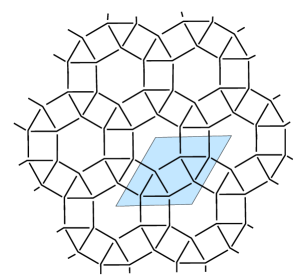
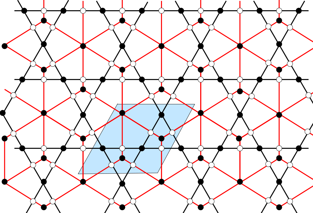
(a)	(b)

Figure 7. (a) Diagram of the biperiodic Rhombitrihexagonal link $\mathcal{R}$, and fundamental domain for $R$. (b) Overlaid graph $G_{\mathcal{R}}^{b}$ and fundamental domain for $G_{R}^{b}$.

Figure 7 shows the rhombitrihexagonal link $\mathcal{R}$ and its alternating quotient link $R$ in $T^{2}\times I$. For the fundamental domain for $G_{\mathcal{R}}^{b}$ as in Figure 7 (middle), $p(z,w)=\det\upkappa(z,w)$ is

$$p_{R}(z,w)=6\,(6-1/w-w-1/z-z-w/z-z/w).$$

Corollary 14.

$$2\pi\,\mathrm{m}(p_{R})=2\pi\log(6)+10{v_{\rm tet}}.$$

Consequently, ${\rm vol}((T^{2}\times I)-R)={\rm vol}^{\lozenge}(R)<2\pi\,\mathrm{m}(p_{R})$.

Proof.

Using Theorem 13, we see that $2\pi\mathrm{m}(p_{R})=2\pi\log(6)+10{v_{\rm tet}}.$

By [17, Theorem 3.5], ${\rm vol}^{\lozenge}(R)={\rm vol}((T^{2}\times I)-R)=10{v_{\rm tet}}+3{v_{\rm oct}}$.

Hence,

$${\rm vol}^{\lozenge}(R)={\rm vol}((T^{2}\times I)-R) = 10\,{v_{\rm tet}}+3\,{v_{\rm oct}}\approx 21.141$$

$$< 10\,{v_{\rm tet}}+2\pi\log(6)\approx 21.407$$

$$= 2\pi\ \mathrm{m}(p_{R}(z,w)).$$

∎

4.4. The link $\mathcal{C}_{0}$

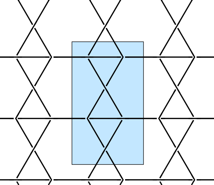
(a)	(b)

Figure 8. (a) Diagram of biperiodic link $\mathcal{C}_{0}$, and fundamental domain for $C_{0}$. (b) Overlaid graph $G_{\mathcal{C}_{0}}^{b}$ and fundamental domain for $G_{C_{0}}^{b}$.

Figure 8(a) shows the biperiodic alternating link $\mathcal{C}_{0}$, and fundamental domain for its alternating quotient link $C_{0}$ in $T^{2}\times I$. For the fundamental domain for $G_{\mathcal{C}_{0}}^{b}$ as in Figure 8(b), we have

$$p_{C_{0}}(z,w)=(-z(w^{2}-4w+1)+w^{2}+4w+1)^{2}.$$

Theorem 15.

$$2\pi\,\mathrm{m}(p_{C_{0}})=16D\left((2+\sqrt{3})i\right)+\frac{8\pi}{3}\log(2+\sqrt{3}).$$

Consequently, $\displaystyle{\rm vol}((T^{2}\times I)-C_{0})={\rm vol}^{\lozenge}(C_{0})<2\pi\,\mathrm{m}(p_{C_{0}})$.

Proof.

Let $q(z,w)=-z(w^{2}-4w+1)+w^{2}+4w+1$. Since $p_{C_{0}}(z,w)=q(z,w)^{2}$, it’s enough to compute $\mathrm{m}(q)$.

In the equation $q(z,w)=0$ solve for $z$ in terms of $w$. Setting $w=e^{i\theta}$ we get

$$|z|=\left|\frac{w+4+w^{-1}}{w-4+w^{-1}}\right|=\left|\frac{\cos\theta+2}{\cos\theta-2}\right|.$$

Hence $|z|\geq 1$ iff $\cos\theta\geq 0$ iff $-\frac{\pi}{2}\leq\theta\leq\frac{\pi}{2}$.

The wedge product leads to

$$w\wedge z= w\wedge\frac{w^{2}+4w+1}{w^{2}-4w+1}$$

$$= w\wedge\frac{(1+(2+\sqrt{3})w)(1+(2-\sqrt{3})w)}{(1-(2+\sqrt{3})w)(1-(2-\sqrt{3})w)}$$

$$= w\wedge(1+(2+\sqrt{3})w)+w\wedge(1+(2-\sqrt{3})w)-w\wedge(1-(2+\sqrt{3})w)$$

$$-w\wedge(1-(2-\sqrt{3})w)$$

$$= (2+\sqrt{3})w\wedge(1+(2+\sqrt{3})w)-(2+\sqrt{3})\wedge(1+(2+\sqrt{3})w)$$

$$+(2-\sqrt{3})w\wedge(1+(2-\sqrt{3})w)-(2-\sqrt{3})\wedge(1+(2-\sqrt{3})w)$$

$$-(2+\sqrt{3})w\wedge(1-(2+\sqrt{3})w)+(2+\sqrt{3})\wedge(1-(2+\sqrt{3})w)$$

$$-(2-\sqrt{3})w\wedge(1-(2-\sqrt{3})w)+(2-\sqrt{3})\wedge(1-(2-\sqrt{3})w).$$

The Mahler measure of the leading coefficient polynomial equals

$$\mathrm{m}(w^{2}-4w+1)=\mathrm{m}\left((w-(2+\sqrt{3}))(w-(2-\sqrt{3}))\right)=\log(2+\sqrt{3}).$$

By applying equation (11), this gives

$$2\pi\,\mathrm{m}(q)-2\pi\log(2+\sqrt{3})= -2D\left(-(2+\sqrt{3})i\right)+2D\left((2+\sqrt{3})i\right)-2D\left(-(2-\sqrt{3})i\right)$$

$$+2D\left((2-\sqrt{3})i\right)+\log(2+\sqrt{3})\int_{-i}^{i}d\arg\left(\frac{1+(2+\sqrt{3})w}{1-(2+\sqrt{3})w}\right)$$

$$+\log(2-\sqrt{3})\int_{-i}^{i}d\arg\left(\frac{1+(2-\sqrt{3})w}{1-(2-\sqrt{3})w}\right).$$

Lemma 16.

We have

(18) $$\int_{-i}^{i}d\arg\left(\frac{1+Rw}{1-Rw}\right)=2\arctan\left(\frac{2}{R-R^{-1}}\right).$$

Proof.

$$I(R):=\int_{-i}^{i}d\arg\left(\frac{1+Rw}{1-Rw}\right)= \int_{-i}^{i}\mathop{\mathrm{Im}}\left(\frac{Rdw}{1+Rw}+\frac{Rdw}{1-Rw}\right)$$

$$= -2\int_{-\pi/2}^{\pi/2}\mathop{\mathrm{Re}}\left(\frac{d\theta}{R^{-1}e^{-i\theta}-Re^{i\theta}}\right)$$

$$= 2(R-R^{-1})\int_{-\pi/2}^{\pi/2}\frac{\cos\theta d\theta}{R^{2}+R^{-2}-2\cos(2\theta)}$$

$$= 2(R-R^{-1})\int_{-1}^{1}\frac{ds}{(R-R^{-1})^{2}+4s^{2}},$$

where we have set $s=\sin\theta$. Therefore, the lemma follows. ∎

By specializing in $R=2+\sqrt{3}$, we obtain

$$I(2+\sqrt{3})=\frac{\pi}{3}=-I(2-\sqrt{3}).$$

By using properties (13) and (14) we finally get

$$2\pi\,\mathrm{m}(q)= 8D\left((2+\sqrt{3})i\right)+2\pi\log(2+\sqrt{3})-\frac{\pi}{3}\log(2+\sqrt{3})+\frac{\pi}{3}\log(2-\sqrt{3})$$

$$= 8D\left((2+\sqrt{3})i\right)+\frac{4\pi}{3}\log(2+\sqrt{3})\approx 10.40161017.$$

Therefore, $2\pi\,\mathrm{m}(p_{C_{0}})=4\pi\,\mathrm{m}(q)\approx 20.80322034.$ By [17, Theorem 3.5],

$${\rm vol}((T^{2}\times I)-C_{0})={\rm vol}^{\lozenge}(C_{0})=20{v_{\rm tet}}\approx 20.29883212$$

Thus, Conjecture 1 is verified for the link $\mathcal{C}_{0}$. ∎

4.5. The link $\mathcal{C}_{1}$

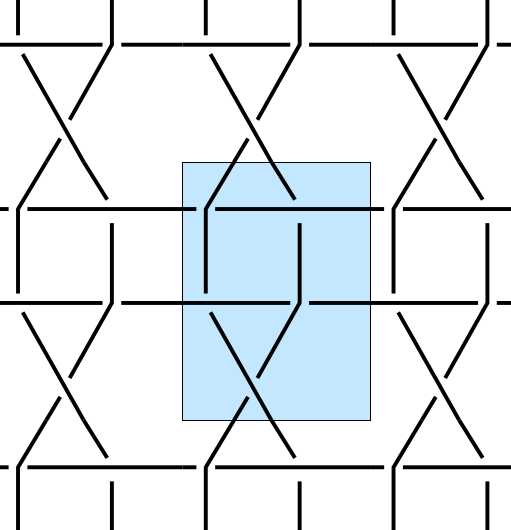
(a)	(b)

Figure 9. (a) Diagram of biperiodic link $\mathcal{C}_{1}$, and fundamental domain for $C_{1}$. (b) Overlaid graph $G_{\mathcal{C}_{1}}^{b}$ and fundamental domain for $G_{C_{1}}^{b}$.

Figure 9(a) shows the biperiodic alternating link $\mathcal{C}_{1}$, and fundamental domain for its alternating quotient link $C_{1}$ in $T^{2}\times I$. For the fundamental domain for $G_{\mathcal{C}_{1}}^{b}$ as in Figure 9(b), we have

$$p_{C_{1}}(z,w)=(1+w^{2})(1-z)^{2}-w(6+20z+6z^{2}).$$

Theorem 17.

$$2\pi\,\mathrm{m}(p_{C_{1}})=16D\left((1+\sqrt{2})i\right)+2\pi\log(1+\sqrt{2}).$$

Consequently, ${\rm vol}((T^{2}\times I)-C_{1})={\rm vol}^{\lozenge}(C_{1})<2\pi\,\mathrm{m}(p_{C_{1}})$.

Proof.

Let

$$p_{1}(z,w)=p_{C_{1}}(z,w^{2})=(w^{4}-6w^{2}+1)z^{2}-2(w^{4}+10w^{2}+1)z+(w^{4}-6w^{2}+1).$$

Then $\mathrm{m}(p_{C_{1}})=\mathrm{m}(p_{1})$. Solving for $z$ in terms of $w$, we get two roots

$$z_{\pm}=\frac{w^{4}+10w^{2}+1\pm 4\sqrt{2}w(w^{2}+1)}{w^{4}-6w^{2}+1}.$$

We need to impose conditions for $|z_{\pm}|\geq 1$. Set $w=e^{i\theta}$. Then

$$z_{\pm}= \frac{w^{2}+10+w^{-2}\pm 4\sqrt{2}(w+w^{-1})}{w^{2}-6+w^{-2}}=\frac{\cos(2\theta)+5\pm 4\sqrt{2}\cos\theta}{\cos(2\theta)-3}$$

$$= \frac{\cos^{2}\theta\pm 2\sqrt{2}\cos\theta+2}{\cos^{2}\theta-2}=\frac{\cos\theta\pm\sqrt{2}}{\cos\theta\mp\sqrt{2}}.$$

Thus, we get $|z_{+}|\geq 1$ iff $\cos\theta\geq 0$ and $|z_{-}|\geq 1$ iff $\cos\theta\leq 0$.

$$w\wedge z_{\pm}= w\wedge\frac{(1+(1\pm\sqrt{2})w)^{2}(1-(1\mp\sqrt{2})w)^{2}}{(1+(1+\sqrt{2})w)(1-(1-\sqrt{2})w)(1+(1-\sqrt{2})w)(1-(1+\sqrt{2})w)}$$

$$= w\wedge\frac{(1+(1\pm\sqrt{2})w)(1-(1\mp\sqrt{2})w)}{(1-(1\pm\sqrt{2})w)(1+(1\mp\sqrt{2})w)}$$

$$= w\wedge(1+(1\pm\sqrt{2})w)+w\wedge(1-(1\mp\sqrt{2})w)-w\wedge(1-(1\pm\sqrt{2})w)$$

$$-w\wedge(1+(1\mp\sqrt{2})w)$$

$$= (1\pm\sqrt{2})w\wedge(1+(1\pm\sqrt{2})w)-(1\pm\sqrt{2})\wedge(1+(1\pm\sqrt{2})w)$$

$$+(1\mp\sqrt{2})w\wedge(1-(1\mp\sqrt{2})w)-(1\mp\sqrt{2})\wedge(1-(1\mp\sqrt{2})w)$$

$$-(1\pm\sqrt{2})w\wedge(1-(1\pm\sqrt{2})w)+(1\pm\sqrt{2})\wedge(1-(1\pm\sqrt{2})w)$$

$$-(1\mp\sqrt{2})w\wedge(1+(1\mp\sqrt{2})w)+(1\mp\sqrt{2})\wedge(1+(1\mp\sqrt{2})w).$$

The Mahler measure of the leading coefficient polynomial equals

$$\mathrm{m}(w^{4}-6w^{2}+1)= \mathrm{m}\left((w+(1+\sqrt{2}))(w-(1-\sqrt{2}))(w+(1-\sqrt{2}))(w-(1+\sqrt{2}))\right)$$

$$= 2\log(1+\sqrt{2}).$$

By putting together the cases of $z_{+}$ and $z_{-}$, and using equation (11), we get

$$2\pi\mathrm{m}(p_{C_{1}})-4\pi\log(1+\sqrt{2})= -4D\left(-(1+\sqrt{2})i\right)+4D\left((1+\sqrt{2})i\right)-4D(-(1-\sqrt{2})i)$$

$$+4D((1-\sqrt{2})i)+2\log(1+\sqrt{2})\int_{-i}^{i}d\arg\left(\frac{1+(1+\sqrt{2})w}{1-(1+\sqrt{2})w}\right)$$

$$+2\log(\sqrt{2}-1)\int_{-i}^{i}d\arg\left(\frac{1+(\sqrt{2}-1)w}{1-(\sqrt{2}-1)w}\right).$$

By equation (18) in Lemma 16,

$$I(1+\sqrt{2})=\frac{\pi}{2}=-I(\sqrt{2}-1).$$

Thus, by properties (13) and (14), we finally obtain

$$2\pi\mathrm{m}(p_{C_{1}})= 16D\left((1+\sqrt{2})i\right)+4\pi\log(1+\sqrt{2})-\pi\log(1+\sqrt{2})+\pi\log(\sqrt{2}-1)$$

$$= 16D\left((1+\sqrt{2})i\right)+2\pi\log(1+\sqrt{2})\approx\ 17.58392561.$$

By [17, Theorem 3.5],

$${\rm vol}((T^{2}\times I)-C_{1})={\rm vol}^{\lozenge}(C_{1})=10{v_{\rm tet}}+2{v_{\rm oct}}\approx\ 17.47714082.$$

Thus, Conjecture 1 is verified for the link $\mathcal{C}_{1}$. ∎

4.6. The family of links $\mathcal{C}_{n}$ (numerical results).

We present some numerical results that generalize the rigorously proven examples $\mathcal{C}_{0}$ and $\mathcal{C}_{1}$.

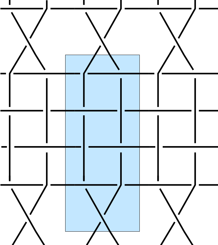
Figure 10. Diagram for one of the biperiodic alternating links $\mathcal{C}_{n}$, and fundamental domain for $C_{n}$. The link $C_{n}$ as shown is for $n=3$.

Let $\mathcal{C}_{n}$ be the family of biperiodic alternating links shown in Figure 8 ($n=0$), Figure 9 ($n=1$), and Figure 10 ($n=3$). For even values of $n$, the fundamental domain like the one shown in Figure  10 does not result in a toroidally alternating link. In these cases, we need to double the fundamental domain, as in Figure 8 for the link $\mathcal{C}_{0}$. Consequently, all the quantities $c(L),\,{\rm vol}(L),\,{\rm vol}^{\lozenge}(L),\,\mathrm{m}(p(z,w))$ are doubled, which does not affect the claim in Conjecture 1.

Conjecture 18.

The characteristic polynomial for the dimer model corresponding to the toroidal link $C_{n}$ is

$$p_{C_{n}}(z,w)=(1+w^{2})(1-z)^{n+1}+(-1)^{n}w\sum_{j=0}^{n+1}\binom{2n+4}{2j+1}z^{j}.$$

If Conjecture 18 holds, then Conjecture 1 would imply that $10{v_{\rm tet}}+2n{v_{\rm oct}}<2\pi\mathrm{m}(p_{C_{n}})$.

$$P_{n}(z,w):=p_{C_{n}}(z^{2},w)=(1+w^{2})(1-z^{2})^{n+1}+(-1)^{n}w\frac{((1+z)^{2n+4}-(1-z)^{2n+4})}{2z}.$$

Then $\mathrm{m}(P_{n})=\mathrm{m}(p_{C_{n}})$. Computing numerical values for $\mathrm{m}(P_{n})$ with Mathematica, we form Table 1. We see that Conjecture 1 is numerically confirmed for the first 12 values of $n$.

$n$	$10{v_{\rm tet}}+2n{v_{\rm oct}}$	$2\pi\mathrm{m}(p_{C_{n}})$
$2$	$24.80486557$	$24.96932402$
$3$	$32.13259032$	$32.27389896$
$4$	$39.46031507$	$39.61527996$
$5$	$46.78803983$	$46.93541034$
$6$	$54.11576458$	$54.26836944$
$7$	$61.44348933$	$61.59270586$
$8$	$68.77121409$	$68.92297116$
$9$	$76.09893884$	$76.2489$ (*)
$10$	$83.42666359$	$83.57804426$
$11$	$90.75438835$	$90.9047$ (*)
$12$	$98.08211310$	$98.23330183$

Table 1. Values for $\mathrm{m}(p_{C_{n}})$. For the two values indicated by (*), we can only get precision up to 4 decimal places.

4.7. Medial graph on the 8-8-4 tiling

Let $\mathcal{K}$ denote biperiodic alternating link whose projection is the medial graph on the 8-8-4 tiling, as shown in Figure 11. Let $K$ be its alternating quotient link in $T^{2}\times I$. In this case, we have

$$p_{K}(z,w)=-w^{2}z^{2}+6w^{2}z+6wz^{2}-w^{2}+28wz-z^{2}+6w+6z-1.$$

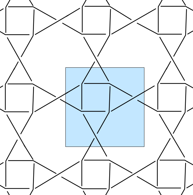
(a)	(b)

Figure 11. (a) Diagram of biperiodic link $\mathcal{K}$, and fundamental domain for $K$. (b) Overlaid graph $G_{\mathcal{K}}^{b}$ and fundamental domain for $G_{K}^{b}$.

Theorem 19.

$$2\pi\,\mathrm{m}(p_{K})=\arccos\left(-\frac{7}{9}\right)\log(17+12\sqrt{2})+8D(i)+4D\left(\frac{\sqrt{7+4\sqrt{2}i}}{3}\right)-4D\left(-\frac{\sqrt{7+4\sqrt{2}i}}{3}\right).$$

Consequently, ${\rm vol}((T^{2}\times I)-K)<{\rm vol}^{\lozenge}(K)<2\pi\,\mathrm{m}(p_{K})$.

Proof.

The curve defined by the zero locus of this polynomial can be parametrized by

$$w= \frac{\sqrt{2}(t^{2}+1)-\sqrt{3}(t^{2}-1)}{\sqrt{2}(t^{2}+1)+\sqrt{3}(t^{2}-1)}=\frac{(2\sqrt{6}-5)\left(t^{2}-\left(5+2\sqrt{6}\right)\right)}{t^{2}-(5-2\sqrt{6})}$$

$$= (2\sqrt{6}-5)\frac{\left(t-(\sqrt{3}+\sqrt{2})\right)\left(t+(\sqrt{3}+\sqrt{2})\right)}{\left(t-(\sqrt{3}-\sqrt{2})\right)\left(t+(\sqrt{3}-\sqrt{2})\right)},$$

$$z= \frac{\sqrt{2}(t^{2}+1)-2\sqrt{3}t}{\sqrt{2}(t^{2}+1)+2\sqrt{3}t}=\frac{t^{2}-\sqrt{6}t+1}{t^{2}+\sqrt{6}t+1}=\frac{\left(t-\frac{\sqrt{3}+1}{\sqrt{2}}\right)\left(t-\frac{\sqrt{3}-1}{\sqrt{2}}\right)}{\left(t+\frac{\sqrt{3}+1}{\sqrt{2}}\right)\left(t+\frac{\sqrt{3}-1}{\sqrt{2}}\right)}.$$

Setting $z=e^{i\theta}$ we get

$$e^{i\theta}=\frac{t^{2}-\sqrt{6}t+1}{t^{2}+\sqrt{6}t+1}\implies(e^{i\theta}-1)t^{2}+(e^{i\theta}+1)\sqrt{6}t+(e^{i\theta}-1)=0\implies t^{2}-i\sqrt{6}\cot\left(\frac{\theta}{2}\right)t+1=0.$$

We continuously choose one of the two roots $t$ for the above polynomial in order to obtain the parametrization. After some numerical computation we conclude that we have to integrate for $\theta\in(0,\pi)$ and $t$ in the complex imaginary segment between $0$ and $-i$, and for $\theta\in(\pi,2\pi)$ and $t$ in the complex imaginary segment between $i$ and $0$.

The general elements that we need to evaluate are

$$-\alpha_{1}\alpha_{2}\alpha_{3}\alpha_{4}\,\left(t+\alpha_{1}\sqrt{2}+\alpha_{2}\sqrt{3}\right)\wedge\left(t+\frac{1+\alpha_{4}\sqrt{3}}{\alpha_{3}\sqrt{2}}\right),\ {\rm and}\ -\alpha_{3}\alpha_{4}\,(2\sqrt{6}-5)\wedge\left(t+\frac{1+\alpha_{4}\sqrt{3}}{\alpha_{3}\sqrt{2}}\right).$$

where $\alpha_{i}\in\{\pm 1\}$ (all possible combinations).

For the terms of the second kind equation (11) yields

$$\log|2\sqrt{6}-5|\left.\arg\left(\frac{t^{2}-\sqrt{6}t+1}{t^{2}+\sqrt{6}t+1}\right)\right|^{-i}_{i}=2\pi\log(5-2\sqrt{6})\approx-14.403772983899.$$

For the terms of the first kind we use Lemma 7 (and ignore terms of the form $(\pm 1)\wedge x$ and $x\wedge(\pm 1)$) to obtain

$$-\alpha_{1}\alpha_{2}\alpha_{3}\alpha_{4}\,\left(t+\alpha_{1}\sqrt{2}+\alpha_{2}\sqrt{3}\right)\wedge\left(t+\frac{1+\alpha_{4}\sqrt{3}}{\alpha_{3}\sqrt{2}}\right)$$

$$= -\alpha_{1}\alpha_{2}\alpha_{3}\alpha_{4}\,\left(\frac{t+\alpha_{1}\sqrt{2}+\alpha_{2}\sqrt{3}}{\alpha_{1}\sqrt{2}+\alpha_{2}\sqrt{3}-\frac{1+\alpha_{4}\sqrt{3}}{\alpha_{3}\sqrt{2}}}\right)\wedge\left(\frac{t+\frac{1+\alpha_{4}\sqrt{3}}{\alpha_{3}\sqrt{2}}}{\alpha_{1}\sqrt{2}+\alpha_{2}\sqrt{3}-\frac{1+\alpha_{4}\sqrt{3}}{\alpha_{3}\sqrt{2}}}\right)$$

$$+\alpha_{1}\alpha_{2}\alpha_{3}\alpha_{4}\,\left(\alpha_{1}\sqrt{2}+\alpha_{2}\sqrt{3}-\frac{1+\alpha_{4}\sqrt{3}}{\alpha_{3}\sqrt{2}}\right)\wedge\left(\frac{t+\alpha_{1}\sqrt{2}+\alpha_{2}\sqrt{3}}{t+\frac{1+\alpha_{4}\sqrt{3}}{\alpha_{3}\sqrt{2}}}\right).$$

The terms in the second line integrate to

$$\alpha_{1}\alpha_{2}\alpha_{3}\alpha_{4}\,\log\left|\alpha_{1}\sqrt{2}+\alpha_{2}\sqrt{3}-\frac{1+\alpha_{4}\sqrt{3}}{\alpha_{3}\sqrt{2}}\right|\left.\arg\left(\frac{t+\alpha_{1}\sqrt{2}+\alpha_{2}\sqrt{3}}{t+\frac{1+\alpha_{4}\sqrt{3}}{\alpha_{3}\sqrt{2}}}\right)\right|^{-i}_{i}.$$

Notice that exchanging the signs of $\alpha_{1}$, $\alpha_{2}$ and $\alpha_{3}$ together amounts to changing $t=\pm i$ to $t=\mp i$ in the argument and does not change the absolute value term inside the logarithm. See Table 2.

				argument	argument	argument	argument
$\alpha_{1}$	$\alpha_{2}$	$\alpha_{3}$	$\alpha_{4}$	at $t=i$	at $t=0^{+}$	at $t=0^{-}$	at $t=-i$
$1$	$1$	$1$	$1$	$\frac{\beta-\pi}{4}$	$0$	$0$	$\frac{\pi-\beta}{4}$
$1$	$-1$	$1$	$1$	$\frac{\pi+\beta}{4}$	$\pi$	$-\pi$	$-\frac{\pi+\beta}{4}$
$1$	$1$	$-1$	$1$	$-\frac{3}{4}\pi$	$-\pi$	$\pi$	$\frac{3}{4}\pi$
$1$	$1$	$1$	$-1$	$\frac{\beta-3\pi}{4}$	$-\pi$	$\pi$	$\frac{3\pi-\beta}{4}$
$1$	$-1$	$-1$	$1$	$-\frac{1}{4}\pi$	$0$	$0$	$\frac{1}{4}\pi$
$1$	$-1$	$1$	$-1$	$\frac{\beta-\pi}{4}$	$0$	$0$	$\frac{\pi-\beta}{4}$
$1$	$1$	$-1$	$-1$	$-\frac{1}{4}\pi$	$0$	$0$	$\frac{1}{4}\pi$
$1$	$-1$	$-1$	$-1$	$\frac{1}{4}\pi$	$\pi$	$-\pi$	$-\frac{1}{4}\pi$

Table 2. Argument at various $t$’s corresponding to values of $\alpha_{i}$’s. Here $\beta=\arccos\left(-\frac{7}{9}\right)\approx 2.4619188346815493642$.

Putting everything together, the integration of the logarithmic terms yields

$$\left(\pi-\beta\right)\log\left|\sqrt{2}+\sqrt{3}-\frac{1+\ \sqrt{3}}{\sqrt{2}}\right|+(\beta-3\pi)\log\left|\sqrt{2}-\sqrt{3}-\frac{1+\sqrt{3}}{\sqrt{2}}\right|+\pi\log\left|\sqrt{2}+\sqrt{3}+\frac{1+\sqrt{3}}{\sqrt{2}}\right|$$

$$+(\beta+\pi)\log\left|\sqrt{2}+\sqrt{3}-\frac{1-\sqrt{3}}{\sqrt{2}}\right|+\pi\log\left|\sqrt{2}-\sqrt{3}+\frac{1+\sqrt{3}}{\sqrt{2}}\right|+\left(\pi-\beta\right)\log\left|\sqrt{2}-\sqrt{3}-\frac{1-\sqrt{3}}{\sqrt{2}}\right|$$

$$+\pi\log\left|\sqrt{2}+\sqrt{3}+\frac{1-\sqrt{3}}{\sqrt{2}}\right|-3\pi\log\left|\sqrt{2}-\sqrt{3}+\frac{1-\sqrt{3}}{\sqrt{2}}\right|.$$

The terms containing $\beta$ yield

$$-\beta\log\left|\sqrt{2}+\sqrt{3}-\frac{1+\ \sqrt{3}}{\sqrt{2}}\right|+\beta\log\left|\sqrt{2}-\sqrt{3}-\frac{1+\sqrt{3}}{\sqrt{2}}\right|+\beta\log\left|\sqrt{2}+\sqrt{3}-\frac{1-\sqrt{3}}{\sqrt{2}}\right|$$

$$-\beta\log\left|\sqrt{2}-\sqrt{3}-\frac{1-\sqrt{3}}{\sqrt{2}}\right|=\beta\log(17+12\sqrt{2})\approx 8.679480937097002.$$

The other terms yield

$$\pi\log\left|\sqrt{2}+\sqrt{3}-\frac{1+\ \sqrt{3}}{\sqrt{2}}\right|-3\pi\log\left|\sqrt{2}-\sqrt{3}-\frac{1+\sqrt{3}}{\sqrt{2}}\right|+\pi\log\left|\sqrt{2}+\sqrt{3}+\frac{1+\sqrt{3}}{\sqrt{2}}\right|$$

$$+\pi\log\left|\sqrt{2}+\sqrt{3}-\frac{1-\sqrt{3}}{\sqrt{2}}\right|+\pi\log\left|\sqrt{2}-\sqrt{3}+\frac{1+\sqrt{3}}{\sqrt{2}}\right|+\pi\log\left|\sqrt{2}-\sqrt{3}-\frac{1-\sqrt{3}}{\sqrt{2}}\right|$$

$$+\pi\log\left|\sqrt{2}+\sqrt{3}+\frac{1-\sqrt{3}}{\sqrt{2}}\right|-3\pi\log\left|\sqrt{2}-\sqrt{3}+\frac{1-\sqrt{3}}{\sqrt{2}}\right|$$

$$= \pi\log(833-588\sqrt{2}-480\sqrt{3}+340\sqrt{6})\approx 3.32810583970523.$$

Finally, the dilogarithm terms are given by

$$\alpha_{1}\alpha_{2}\alpha_{3}\alpha_{4}D\left(\frac{-t-\frac{1+\alpha_{4}\sqrt{3}}{\alpha_{3}\sqrt{2}}}{\alpha_{1}\sqrt{2}+\alpha_{2}\sqrt{3}-\frac{1+\alpha_{4}\sqrt{3}}{\alpha_{3}\sqrt{2}}}\right)$$

Notice that exchanging the signs of $\alpha_{1}$, $\alpha_{2}$, and $\alpha_{3}$ together amounts to changing the sign of $t$. This can be combined with formulas in equations (13) and (14) to obtain

$$4D\left(\frac{i-\frac{1+\sqrt{3}}{\sqrt{2}}}{\sqrt{2}+\sqrt{3}-\frac{1+\sqrt{3}}{\sqrt{2}}}\right)-4D\left(\frac{i-\frac{1+\sqrt{3}}{\sqrt{2}}}{\sqrt{2}-\sqrt{3}-\frac{1+\sqrt{3}}{\sqrt{2}}}\right)-4D\left(\frac{i+\frac{1+\sqrt{3}}{\sqrt{2}}}{\sqrt{2}+\sqrt{3}+\frac{1+\sqrt{3}}{\sqrt{2}}}\right)$$

$$-4D\left(\frac{i-\frac{1-\sqrt{3}}{\sqrt{2}}}{\sqrt{2}+\sqrt{3}-\frac{1-\sqrt{3}}{\sqrt{2}}}\right)+4D\left(\frac{i+\frac{1+\sqrt{3}}{\sqrt{2}}}{\sqrt{2}-\sqrt{3}+\frac{1+\sqrt{3}}{\sqrt{2}}}\right)+4D\left(\frac{i-\frac{1-\sqrt{3}}{\sqrt{2}}}{\sqrt{2}-\sqrt{3}-\frac{1-\sqrt{3}}{\sqrt{2}}}\right)$$

$$+4D\left(\frac{i+\frac{1-\sqrt{3}}{\sqrt{2}}}{\sqrt{2}+\sqrt{3}+\frac{1-\sqrt{3}}{\sqrt{2}}}\right)-4D\left(\frac{i+\frac{1-\sqrt{3}}{\sqrt{2}}}{\sqrt{2}-\sqrt{3}+\frac{1-\sqrt{3}}{\sqrt{2}}}\right)$$

$$\approx 4\cdot 2.77301284617524\approx 11.092051384700.$$

By applying the five-term relation and identities such as the following

$$\frac{-i-\frac{1+\sqrt{3}}{\sqrt{2}}}{\sqrt{2}-\sqrt{3}-\frac{1+\sqrt{3}}{\sqrt{2}}}=1-\frac{1}{\frac{1-\frac{i+\frac{1-\sqrt{3}}{\sqrt{2}}}{\sqrt{2}-\sqrt{3}+\frac{1-\sqrt{3}}{\sqrt{2}}}}{1-\frac{i-\frac{1-\sqrt{3}}{\sqrt{2}}}{\sqrt{2}+\sqrt{3}-\frac{1-\sqrt{3}}{\sqrt{2}}}\frac{i+\frac{1-\sqrt{3}}{\sqrt{2}}}{\sqrt{2}-\sqrt{3}+\frac{1-\sqrt{3}}{\sqrt{2}}}}},$$

one can prove

$$D\left(\frac{i-\frac{1-\sqrt{3}}{\sqrt{2}}}{\sqrt{2}+\sqrt{3}-\frac{1-\sqrt{3}}{\sqrt{2}}}\right)+D\left(\frac{i+\frac{1-\sqrt{3}}{\sqrt{2}}}{\sqrt{2}-\sqrt{3}+\frac{1-\sqrt{3}}{\sqrt{2}}}\right)=D\left(\frac{i-\frac{1+\sqrt{3}}{\sqrt{2}}}{\sqrt{2}-\sqrt{3}-\frac{1+\sqrt{3}}{\sqrt{2}}}\right)+D\left(\frac{i+\frac{1+\sqrt{3}}{\sqrt{2}}}{\sqrt{2}+\sqrt{3}+\frac{1+\sqrt{3}}{\sqrt{2}}}\right)$$

and

$$D\left(\frac{i-\frac{1+\sqrt{3}}{\sqrt{2}}}{\sqrt{2}+\sqrt{3}-\frac{1+\sqrt{3}}{\sqrt{2}}}\right)+D\left(\frac{i+\frac{1+\sqrt{3}}{\sqrt{2}}}{\sqrt{2}-\sqrt{3}+\frac{1+\sqrt{3}}{\sqrt{2}}}\right)=D\left(\frac{i-\frac{1-\sqrt{3}}{\sqrt{2}}}{\sqrt{2}-\sqrt{3}-\frac{1-\sqrt{3}}{\sqrt{2}}}\right)+D\left(\frac{i+\frac{1-\sqrt{3}}{\sqrt{2}}}{\sqrt{2}+\sqrt{3}+\frac{1-\sqrt{3}}{\sqrt{2}}}\right).$$

This allows us to simplify the dilogarithm terms as

$$8D\left(\frac{i-\frac{1+\sqrt{3}}{\sqrt{2}}}{\sqrt{2}+\sqrt{3}-\frac{1+\sqrt{3}}{\sqrt{2}}}\right)-8D\left(\frac{i-\frac{1+\sqrt{3}}{\sqrt{2}}}{\sqrt{2}-\sqrt{3}-\frac{1+\sqrt{3}}{\sqrt{2}}}\right)-8D\left(\frac{i+\frac{1+\sqrt{3}}{\sqrt{2}}}{\sqrt{2}+\sqrt{3}+\frac{1+\sqrt{3}}{\sqrt{2}}}\right)+8D\left(\frac{i+\frac{1+\sqrt{3}}{\sqrt{2}}}{\sqrt{2}-\sqrt{3}+\frac{1+\sqrt{3}}{\sqrt{2}}}\right).$$

By using the identity (16) we see that the dilogarithm terms equal

$$8D(i)+4D\left(\frac{\sqrt{7+4\sqrt{2}i}}{3}\right)-4D\left(-\frac{\sqrt{7+4\sqrt{2}i}}{3}\right).$$

Then we have to add everything as well as the Mahler measure of $z^{2}-6z+1$ which is

$$2\pi\mathrm{m}(z^{2}-6z+1)=2\pi\log(3+2\sqrt{2})\approx 2\pi\cdot 1.76274717403908\approx 11.075667144194722.$$

Putting everything together and collapsing terms, we obtain

$$2\pi\mathrm{m}(p_{K})= \arccos\left(-\frac{7}{9}\right)\log(17+12\sqrt{2})+8D(i)+4D\left(\frac{\sqrt{7+4\sqrt{2}i}}{3}\right)-4D\left(-\frac{\sqrt{7+4\sqrt{2}i}}{3}\right)$$

$$\approx 19.771532321797992256575200922336735211.$$

Finally,

$${\rm vol}^{\lozenge}(K)={\rm vol}(B_{8})+{\rm vol}(B_{4})+4{\rm vol}(B_{3})\approx 7.8549+3.6638+4\times 2.0298=19.6379.$$

Using SnapPy [21] inside Sage to verify the computation rigorously, we verified that

$${\rm vol}((T^{2}\times I)-K)\approx 19.559.$$

Thus, the link $\mathcal{K}$ satisfies Conjecture 1, as well as inequality (5) within a range of 0.4%,

$${\rm vol}((T^{2}\times I)-K)<{\rm vol}^{\lozenge}(K)<2\pi\,\mathrm{m}(p_{K}).$$

∎

We remark that, except for the link $\mathcal{K}$, the logarithmic terms in the formulas for $2\pi\mathrm{m}(p)$ for all the other links above are of the form $q\pi\log(\alpha)$, where $q$ is a rational number and $\alpha$ is an algebraic number. In Theorem 19, we have instead a term of the form $\arccos\left(-\frac{7}{9}\right)\log(\alpha)$. The parameter $-\frac{7}{9}$ is also involved in the arguments for the dilogarithm terms, since

$$\frac{\sqrt{7+4\sqrt{2}i}}{3}=\exp\left(\frac{i}{2}\left(\pi-\arccos\left(-\frac{7}{9}\right)\right)\right).$$

References

• [1] Colin Adams, Bipyramids and bounds on volumes of hyperbolic links, Topology Appl. 222 (2017), 100–114.
• [2] Colin Adams, Carlos Albors-Riera, Beatrix Haddock, Zhiqi Li, Daishiro Nishida, and Luya Wang, Hyperbolicity of links in thickened surfaces, arXiv:1802.05770 [math.GT], 2018.
• [3] Colin Adams, Thomas Fleming, Michael Levin, and Ari M. Turner, Crossing number of alternating knots in $S\times I$, Pacific J. Math. 203 (2002), no. 1, 1–22.
• [4] Peter Borwein, Edward Dobrowolski, and Michael J. Mossinghoff, Lehmer’s problem for polynomials with odd coefficients, Ann. of Math. (2) 166 (2007), no. 2, 347–366.
• [5] D. Boyd and F. Rodriguez-Villegas, Mahler’s measure and the dilogarithm. I, Canad. J. Math. 54 (2002), no. 3, 468–492.
• [6] D. Boyd, F. Rodriguez-Villegas, and N. Dunfield, Mahler’s measure and the dilogarithm (II), arXiv:math.NT/0308041.
• [7] David W. Boyd, Speculations concerning the range of Mahler’s measure, Canad. Math. Bull. 24 (1981), no. 4, 453–469.
• [8] by same author, Mahler’s measure and special values of $L$-functions, Experiment. Math. 7 (1998), no. 1, 37–82.
• [9] by same author, Mahler’s measure and invariants of hyperbolic manifolds, Number theory for the millennium, I (Urbana, IL, 2000), A K Peters, Natick, MA, 2002, pp. 127–143.
• [10] Robert Breusch, On the distribution of the roots of a polynomial with integral coefficients, Proc. Amer. Math. Soc. 2 (1951), 939–941.
• [11] Stephan D. Burton, The determinant and volume of 2-bridge links and alternating 3-braids, New York J. Math. 24 (2018), 293–316.
• [12] Abhijit Champanerkar, A-polynomial and Bloch invariants of hyperbolic 3-manifolds, ProQuest LLC, Ann Arbor, MI, 2003, Thesis (Ph.D.)–Columbia University. Preprint available at http://www.math.csi.cuny.edu/~abhijit/research.html.
• [13] Abhijit Champanerkar and Ilya Kofman, Determinant density and biperiodic alternating links, New York J. Math. 22 (2016), 891–906.
• [14] Abhijit Champanerkar, Ilya Kofman, and Jessica S. Purcell, Density spectra for knots, J. Knot Theory Ramifications 25 (2016), no. 3, 1640001, 11.
• [15] by same author, Geometrically and diagrammatically maximal knots, J. Lond. Math. Soc. (2) 94 (2016), no. 3, 883–908.
• [16] by same author, Volume bounds for weaving knots, Algebr. Geom. Topol. 16 (2016), no. 6, 3301–3323.
• [17] by same author, Geometry of biperiodic alternating links, arXiv:1802.05343 [math.GT], 2018.
• [18] David Cimasoni, The geometry of dimer models, Winter Braids Lect. Notes 1 (2014), no. Winter Braids IV (Dijon, 2014), Exp. No. 2, 14.
• [19] Moshe Cohen, Oliver T. Dasbach, and Heather M. Russell, A twisted dimer model for knots, Fund. Math. 225 (2014), no. 1, 57–74.
• [20] D. Cooper, M. Culler, H. Gillet, D. Long, and P. Shalen, Plane curves associated to character varieties of $3$-manifolds, Invent. Math. 118 (1994), 47–84.
• [21] Marc Culler, Nathan M. Dunfield, Matthias Goerner, and Jeffrey R. Weeks, SnapPy, a computer program for studying the geometry and topology of $3$-manifolds, Available at http://snappy.computop.org.
• [22] E. Dobrowolski, On a question of Lehmer and the number of irreducible factors of a polynomial, Acta Arith. 34 (1979), no. 4, 391–401.
• [23] Nathan Dunfield, http://www.math.uiuc.edu/~nmd/preprints/misc/dylan/index.html.
• [24] Antonin Guilloux and Julien Marché, Volume function and Mahler measure of exact polynomials, arXiv:1804.01395 [math.GT], 2018.
• [25] Joshua A. Howie and Jessica S. Purcell, Geometry of alternating links on surfaces, arXiv:1712.01373 [math.GT], 2017.
• [26] R. Kenyon, The Laplacian and Dirac operators on critical planar graphs, Invent. Math. 150 (2002), no. 2, 409–439.
• [27] R. Kenyon, A. Okounkov, and S. Sheffield, Dimers and amoebae, Ann. of Math. (2) 163 (2006), no. 3, 1019–1056.
• [28] Richard Kenyon, Lectures on dimers, Statistical mechanics, IAS/Park City Math. Ser., vol. 16, Amer. Math. Soc., Providence, RI, 2009, pp. 191–230.
• [29] Matilde Lalín, Mahler measure and volumes in hyperbolic space, Geom. Dedicata 107 (2004), 211–234.
• [30] W. Lawton, A problem of Boyd concerning geometric means of polynomials, J. Number Theory 16 (1983), no. 3, 356–362.
• [31] D. H. Lehmer, Factorization of certain cyclotomic functions, Ann. of Math. (2) 34 (1933), no. 3, 461–479.
• [32] W. B. Raymond Lickorish, An introduction to knot theory, Graduate Texts in Mathematics, vol. 175, Springer-Verlag, New York, 1997.
• [33] J. Rafael Sendra, Franz Winkler, and Sonia Pérez-Díaz, Rational algebraic curves, Algorithms and Computation in Mathematics, vol. 22, Springer, Berlin, 2008, A computer algebra approach.
• [34] C. Smyth, On the product of the conjugates outside the unit circle of an algebraic integer, Bull. London Math. Soc. 3 (1971), 169–175.
• [35] by same author, On measures of polynomials in several variables, Bull. Austral. Math. Soc. 23 (1981), no. 1, 49–63.
• [36] C. J. Smyth, A Kronecker-type theorem for complex polynomials in several variables, Canad. Math. Bull. 24 (1981), no. 4, 447–452.
• [37] Alexander Stoimenow, Graphs, determinants of knots and hyperbolic volume, Pacific J. Math. 232 (2007), no. 2, 423–451.
• [38] Sam Vandervelde, The Mahler measure of parametrizable polynomials, J. Number Theory 128 (2008), no. 8, 2231–2250.
• [39] D. Zagier, The remarkable dilogarithm, J. Math. Phys. Sci. 22 (1988), no. 1, 131–145.