Quadratic Time Algorithms Appear to be Optimal for Sorting Evolving Data

Abstract

We empirically study sorting in the evolving data model. In this model, a sorting algorithm maintains an approximation to the sorted order of a list of data items while simultaneously, with each comparison made by the algorithm, an adversary randomly swaps the order of adjacent items in the true sorted order. Previous work studies only two versions of quicksort, and has a gap between the lower bound of $\Omega(n)$ and the best upper bound of $O(n\log\log n)$. The experiments we perform in this paper provide empirical evidence that some quadratic-time algorithms such as insertion sort and bubble sort are asymptotically optimal for any constant rate of random swaps. In fact, these algorithms perform as well as or better than algorithms such as quicksort that are more efficient in the traditional algorithm analysis model.

1 Introduction

In the traditional Knuthian model [11], an algorithm takes an input, runs for some amount of time, and produces an output. Characterizing an algorithm in this model typically involves providing a function, $f(n)$, such that the running time of the algorithm can be bounded asymptotically as being $O(f(n))$ on average, with high probability (w.h.p.), or in the worst case. Although this has proven to be an extremely useful model for general algorithm design and analysis, there are nevertheless interesting scenarios where it doesn’t apply.

1.1 The Evolving Data Model

One scenario where the Knuthian model doesn’t apply is for applications where the input data is changing while an algorithm is processing it, which has given rise to the evolving data model [1]. In this model, input changes are coming so fast that it is hard for an algorithm to keep up, much like Lucy in the classic conveyor belt scene in the TV show, I Love Lucy. Thus, rather than produce a single output, as in the Knuthian model, an algorithm in the evolving data model dynamically maintains an output instance over time. The goal of an algorithm in this model is to efficiently maintain its output instance so that it is “close” to the true output at that time. Therefore, analyzing an algorithm in the evolving data model involves defining a distance metric for output instances, parameterizing how input mutations occur over time, and characterizing how well an algorithm can maintain its output instance relative to this distance and these parameters for various types of input mutations.

The goal of a sorting algorithm in the evolving data model, then, is to maintain an output order close to the true total order even as it is mutating. For example, the list could be an ordering of political candidates, tennis players, movies, songs, or websites, which is changing as the ranking of these items is evolving, e.g., see [6]. In such contexts, performing a comparison of two elements is considered somewhat slow and expensive, in that it might involve a debate between two candidates, a match between two players, or an online survey or A/B test [5] comparing two movies, songs, or websites. In this model, a comparison-based sorting algorithm would therefore be executing at a rate commensurate with the speed in which the total order is changing, i.e., its mutation rate. Formally, to model this phenomenon, each time an algorithm performs a comparison, we allow for an adversary to perform some changes to the true ordering of the elements.

There are several different adversaries one might consider with respect to mutations that would be anticipated after a sorting algorithm performs a comparison. For example, an adversary (who we call the uniform adversary) might choose $r>0$ consecutive pairs of elements in the true total order uniformly at random and swap their relative order. Indeed, previous work [1] provided theoretical analyses for the uniform adversary for the case when $r$ is a constant. Another type of adversary (who we call the hot spot adversary) might choose an element, $x$, in the total order and repeatedly swap $x$ with a predecessor or successor each time a random “coin flip” comes up “tails,” not stopping until the coin comes up “heads.”

A natural distance metric to use in this context is the Kendall tau distance [10], which counts the number of inversions between a total ordering of $n$ distinct elements and a given list of those elements. That is, a natural goal of a sorting algorithm in the evolving data model is to minimize the Kendall tau distance for its output list over time.

Here, we consider the empirical performance of sorting algorithms in the evolving data model. Whereas previous work looked only at quicksort with respect to theoretical analyses against the uniform adversary, we are interested in this paper in the “real-world” performance of a variety of sorting algorithms with respect to multiple types of adversaries in the evolving data model. Of particular interest are any experimental results that might be counter-intuitive or would highlight gaps in the theory.

1.2 Previous Work on Evolving Data

The evolving data model was introduced by Anagnostopoulos et al. [1], who study sorting and selection problems with respect to an evolving total order. They prove that quicksort maintains a Kendall tau distance of $O(n\log n)$ w.h.p. with respect to the true total order, against a uniform adversary that performs a small constant number of random swaps for every comparison made by the algorithm. Furthermore, they show that a batched collection of quicksort algorithms operating on overlapping blocks can maintain a Kendall tau distance of $O(n\log\log n)$ against this same adversary. We are not aware of previous experimental work on sorting in the evoloving data model. We are also not aware of previous work, in general, in the evolving data model for other sorting algorithms or for other types of adversaries.

In addition to this work on sorting, several papers have considered other problems in the evolving data model. Kanade et al. [9] study stable matching with evolving preferences. Huang et al. [8] present how to select the top-$k$ elements from an evolving list. Zhang and Li [12] consider how to find shortest paths in an evolving graph. Anagnostopoulos et al. [2] study $(s,t)$-connectivity and minimum spanning trees in evolving graphs. Bahmani et al. [3] give several PageRank algorithms for evolving graphs and they analyze these algorithms both theoretically and experimentally. To our knowledge, this work is the only previous experimental work for the evolving data model.

1.3 Our Results

In this paper, we provide an experimental investigation of sorting in the evolving data model. The starting point for our work is the previous theoretical work [1] on sorting in the evolving data model, which only studies quicksort. Thus, our first result is to report on experiments that address whether these previous theoretical results actually reflect real-world performance.

In addition, we experimentally investigate a number of other classic sorting algorithms to empirically study whether these algorithms lead to good sorting algorithms for evolving data and to study how sensitive they are to parameters in the underlying evolving data model. Interestingly, our experiments provide empirical evidence that quadratic-time sorting algorithms, including bubble sort, cocktail sort, and insertion sort, can outperform more sophisticated algorithms, such as quicksort and even the batched parallel blocked quicksort algorithm of Anagnostopoulos et al. [1], in practice. Furthermore, our results also show that even though these quadratic-time algorithms perform compare-and-swap operations only for adjacent elements at each time step, they are nevertheless robust to increasing the rate, $r$, at which random swaps occur in the underlying list for every comparison done by the algorithm. That is, our results show that these quadratic-time algorithms are robust even in the face of an adversary who can perform many swaps for each of an algorithm’s comparisons. Moreover, this robustness holds in spite of the fact that, in such highly volatile situations, each element is, on average, moved more often by random swaps than by the sorting algorithm’s operations.

We also introduce the hot spot adversary and study sorting algorithms in the evolving data model with respect to this adversary. Our experiments provide evidence that these sorting algorithms have similar robustness against the hot spot adversary as they do against the uniform adversary. Finally, we show that the constant factors in the Kendall tau distances maintained by classic quadratic-time sorting algorithms appear to be quite reasonable in practice. Therefore, we feel our experimental results are arguably surprising, in that they show the strengths of quadratic-time algorithms in the evolving data model, in spite of the fact that these algorithms are much maligned because of their poor performance in the traditional Knuthian model.

With respect to the organization of our paper, section 2 formally introduces the evolving sorting model as well as the algorithms we consider in this paper. section 3 describes the experiments we performed and presents our results.

2 Preliminaries

Let us begin by formally defining the evolving data model for sorting, based on the pioneering work of Anagnostopoulos et al. [1]. We assume that there are $n$ distinct elements that belong to a total order relation, “$<$”. During each time step, a sorting algorithm is allowed to perform one comparison of a pair of elements and then an adversary is allowed to perform some random swaps between adjacent elements in the true total order. In this paper, we consider two types of adversaries:

1. The uniform adversary. This adversary performs a number, $r>0$, of swaps between pairs of adjacent elements in the true total order, where these pairs are chosen uniformly at random and independently for each of the $r$ swaps.

2. The hot spot adversary. This adversary chooses an element, $x$, in the total order and then randomly choose a direction, up or down. The adversary then randomly chooses a bit, $b$. If this bit is $0$, he swaps $x$ with its predecessor (resp., successor), depending on the chosen direction, and repeats this process with a new random bit, $b$. If $b=1$, he stops swapping $x$.

We denote the state of the list the algorithm maintains at time $t$ with $\ell_{t}$ and the state of the unknown true ordering with $\ell^{\prime}_{t}$. If the time step is clear from the context or is the most current step, then we may drop the subscript, $t$. The main type of adversary that we consider is the same as that considered in Anagnostopoulos et al. [1]; namely, what we are calling the uniform adversary. Note that with this adversary, after each comparison, a uniformly random adjacent pair of elements in $\ell^{\prime}$ exchange positions and this process is repeated independently for a total of $r>0$ swaps. We call each such change to $\ell^{\prime}$ a swap mutation. With respect to the hot spot adversary, we refer to the change made to $\ell^{\prime}$ as a hot spot mutation, i.e., where an element is picked uniformly at random and flips an unbiased coin to pick left or right, and then an unbiased coin is flipped until it comes up heads and the element is swapped in the chosen direction that many times.

Note that with either adversary, a sorting algorithm cannot hope to correctly maintain the true total order at every step, for at least the reason that it has no knowledge of how the most recent mutation affected the underlying order. Instead, a sorting algorithm’s goal is to maintain a list of the $n$ elements that has a small Kendall tau distance, which counts the number of inversions relative to the underlying total order.

We abuse the names of the classical sorting algorithms to refer to evolving sorting algorithms that repeatedly run that classical algorithm. For instance, the insertion sort evolving sorting algorithm repeatedly runs the classical in-place insertion sort algorithm. We refer to each individual run of a classical sorting algorithm as a round.

In this paper, we consider several classical sorting algorithms, which are summarized in simplified form below (see [4, 7] for details and variations on these algorithms):

• Bubble sort. For $i=1,\ldots,n-1$, repeatedly compare the elements at positions $i$ and $i+1$, swapping them if they are out of order. Repeat $n-1$ times.

• Cocktail sort. For $i=1,\ldots,n-1$, repeatedly compare the elements at positions $i$ and $i+1$, swapping them if they are out of order. Then do the same for $i=n-1,\ldots,1$. Repeat $(n-2)/2$ times.

• Insertion sort. For $i=2,\ldots,n$, compare the element, $x$, at position $i$ with its predecessor, swapping them if they are out of order. Then repeat this process again with $x$ (at its new position) until it reaches the beginning of the list or isn’t swapped. Repeat $n-2$ times.

• Quicksort. Randomly choose a pivot, $x$, in the list and divide the list inplace as the elements that are less than or equal to $x$ and the elements that are greater than $x$. Recursively process each sublist if it has at least two elements.

We also consider the following algorithm due to Anagnostopoulos et al. [1]:

• Block sort. Divide the list into overlapping blocks of size $O(\log n)$. Alternate between steps of quicksort on the entire list and steps of quicksort on each block.

There are no theoretical results on the quality of bubble, cocktail, or insertion sort in the evolving data model. Anagnostopoulos et al. [1] showed that quicksort achieves $\Theta(n\log n)$ inversions w.h.p. for any small constant, $r$, of swap mutations. Anagnostopoulos et al. [1] also showed that block sort achieves $\Theta(n\log\log n)$ inversions w.h.p. for any small constant, $r$, of swap mutations.

These algorithms can be classified in two ways. First, they can be separated into the worst-case quadratic-time sorting algorithms (bubble sort, cocktail sort, and insertion sort) and the more efficient algorithms (quicksort and block sort), with respect to their performance in the Knuthian model. Second, they can also be separated into two classes based on the types of comparisons they perform and how they update $\ell$. Bubble sort, cocktail sort, and insertion sort consist of compare-and-swap operations of adjacent elements in $\ell$ and additional bookkeeping, while quicksort and block sort perform comparisons of elements that are currently distant in $\ell$ and only update $\ell$ after the completion of some subroutines.

During the execution of these algorithms, the Kendall tau distance does not converge to a single number. For example, the batch update behavior of quicksort causes the Kendall tau distance to oscillate each time a round of quicksort finishes. Nevertheless, for all of the algorithms, the Kendall tau distance empirically reaches a final repetitive behavior. We call this the steady behavior for the algorithm and judge algorithms by the average number of inversions once they reach their steady behavior. We call the time it takes an algorithm to reach its steady behavior its convergence time. Every algorithm’s empirical convergence time is at most $n^{2}$ steps.

3 Experiments

The main goal of our experimental framework is to address the following questions:

1. Do quadratic-time algorithms actually perform as well as or better than quicksort variants on evolving data using swap mutations, e.g., for reasonable values of $n$?

2. What is the nature of the convergence of sorting algorithms on evolving data, e.g., how quickly do they converge and how much do they oscillate once they converge?

3. How robust are the algorithms to increasing the value of $r$ for swap mutations?

4. How much does an algorithm’s convergence behavior and steady behavior depend on the list’s initial configuration (e.g., randomly scrambled or initially sorted)?

5. How robust are the algorithms to a change in the mutation behavior, such as with the hot spot adversary?

6. What is the fraction of random swaps that actually improve Kendall tau distance?

We present results below that address each of these questions.

3.1 Experimental Setup

We implemented the various algorithms that we study in C++11 and our software is available on Github. Randomness for experiments was generated using the C++ default_engine and in some cases using the C random engine. In the evolving data model, each time step corresponds to one comparison step in an algorithm, which is followed by a mutation performed by an adversary. Therefore, our experiments measure time by the number of comparisons performed. Of course, all the algorithms we study are comparison-based; hence, their number of comparisons correlates with their wall-clock runtimes. To measure Kendall tau distances, we sample the number of inversions every $n/20$ comparisons, where $n$ is the size of a list. We terminate a run after $n^{2}$ time steps and well after the algorithm has reached its steady behavior. The experiments primarily used random swap mutations; hence, we omit mentioning the mutation type unless we are using hot spot mutations.

Anagnostopoulos et al. [1] does not give an exact block size for their block sort algorithm except in terms of several unknown constants. In our block sort implementation, the block size chosen for block sort is the first even number larger than $10\ln n$ that divides $n$. Because all of the $n$ in our experiments are multiples of $1000$, the block size is guaranteed to be between $10\ln n$ and $100\ln n$.

3.2 General Questions Regarding Convergence Behavior

We begin by empirically addressing the first two questions listed above, which concern the general convergence behavior of the different algorithms. Figure 1 shows Kendall tau distance achieved by the various algorithms we studied as a function of the algorithm’s execution time, against the uniform adversary (i.e., with random swap mutations), for the case when $r=1$ and $n=1000$ starting from a uniformly shuffled list.

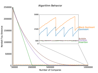
Figure 1: Behavior of the algorithms starting from a shuffled list. The plot shows Kendall tau distance as a function of an algorithm’s execution, i.e., number of comparisons, with random swap mutations for $r=1$. We also show an enlarged portion of the tail-end steady behaviors.

The quadratic time algorithms run continuous passes on the list and every time they find two elements in the wrong order they immediately swap them. That is, they are local in scope, at each step fixing inversions by swapping adjacent elements. They differ in their approach, but once each such algorithm establishes a balance between the comparisons performed by the algorithm and the mutations performed by the uniform adversary, their Kendall tau numbers don’t differ significantly. These algorithms have very slow convergence because they only compare adjacent elements in the list and so fix at most one inversion with each comparison. The Kendall tau behavior of the quicksort algorithms, on the other hand, follow an oscillating pattern of increasing Kendall tau distance until a block (or recursive call) is finished, at which point $\ell$ is quickly updated, causing a large decrease in Kendall tau distance.

As can be seen, the convergence behavior of the algorithms can be classified into two groups. The first group consists of the two quicksort variants, which very quickly converge to steady behaviors that oscillate in a small range. The second group consists of the quadratic-time algorithms, which converge more slowly, but to much smaller Kendall tau distances and with no clear oscillating behavior. More interestingly, the quadratic-time algorithms all converge to the same tight range and this range of values is better than the wider range of Kendall tau distances achieved by the quicksort algorithms. Thus, our first experimental result already answers our main question, namely, that these quadratic-time algorithms appear to be optimal for sorting evolving data and this behavior is actually superior in the limit to the quicksort variants.

Given enough time, however, all three quadratic-time algorithms maintain a consistent Kendall tau distance in the limit. Of the three quadratic-time algorithms, the best performer is insertion sort, followed by cocktail sort and then bubble sort. The worst algorithm in our first batch of experiments was block quicksort. This may be because $n=1000$ is too small for the theoretically proven $O(n\log\log n)$ Kendall tau distance to hold.

3.3 Convergence Behavior as a Function of $r$

Regardless of the categories, after a sufficient number of comparisons, all the algorithms empirically reach a steady behavior where the distance between $\ell$ and $\ell^{\prime}$ follows a cyclic pattern over time. This steady behavior depends on the algorithm, the list size, $n$, and the number of random swaps, $r$, per comparison, but it is visually consistent across many different runs and starting configurations.

Our next set of experiments, therefore, are concerned with studying convergence behavior as a function of $n$ and $r$. We show in Figure 2 the convergence values comparing insertion sort and quicksort, as a ratio, $K/n$, of the steady-state Kendall tau distance, $K$ (averaged across multiple samples once an algorithm has reached its steady behavior), and the list size, $n$.

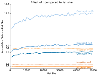
Figure 2: Convergence ratios as a function of list size, $n$, and number of random swaps, $r$, per comparison. The vertical axis shows the ratio, $K/n$, where $K$ is the average Kendall tau value (number of inversions) in the steady behavior, and the horizontal axis shows the number of elements, $n$. The curves show the behaviors of insertion sort and quicksort for $r\in\{1,2,10\}$.

As can be seen from the plots, for these values of $r$, insertion sort consistently beats quicksort in terms of the Kendall tau distance it achieves, and this behavior is surprisingly robust even as $n$ grows. Moreover, all of the quadratic-time algorithms that we studied achieved similar Kendall-tau-to-size ratios that were consistently competitive with both quicksort and block sort. In the appendix, we give a table showing specific ratio values for these algorithms for a variety of chosen values for $r$. Our results show that for values of $r$ larger than $50$, the quicksort variants tend to perform better than the quadratic-time algorithms, but the quadratic time algorithms nevertheless still converge to reasonable ratios. We show in Table 1, which is also given in the appendix, specific convergence values for different values of $r$, from $0$ to $10$, for insertion sort and quicksort.

3.4 Starting Configurations

The quadratic time algorithms all approach their steady behavior in a similar manner, namely, at an approximately constant rate attenuated by $r$. Thus, we also empirically investigated how long each algorithm requires to reach a steady behavior starting from a variety of different start configurations.

Because both quicksort and block sort begin with a quicksort round, their Kendall tau distance drops quickly after $O(n\log n)$ comparisons. The other algorithms require a number of comparisons proportional to the initial distance from the steady-state value. For example, see Table 2 in the appendix, which shows that insertion sort’s steady behavior when $r=1$ is roughly $n/2$ inversions. When the initial state of a list has $I$ inversions, the number of comparisons that insertion sort requires to reach the steady behavior is approximately $4|I-n/2|$. Thus, if the list is initially sorted, insertion sort will take approximately $2n$ comparisons to reach its steady behavior. Moreover, increasing $r$ does not seem to affect the convergence rate significantly. Figure 3 shows a plot illustrating the convergence behavior of insertion sort and quicksort for a variety of different starting configurations.

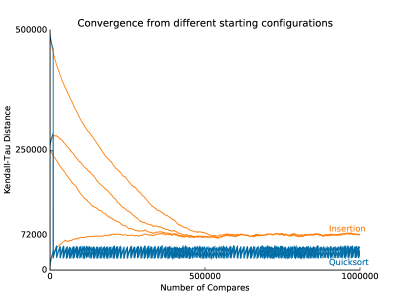
Figure 3: Even for a large $r=256$ over only 1000 elements the algorithms quickly converge to a steady behavior. The plots show the Kendal tau distances achieved for insertion sort and quicksort for four starting configurations of increasing complexity: (i) initially sorted, (ii) random shuffle, (iii) half cyclical shift of a sorted list, and (iv) a list in reverse order.

Our experiments show that, as expected, the convergence of insertion sort is sensitive to the starting configuration, whereas quicksort is not. Primed with this knowledge, these results justify our starting from a sorted configuration in our subsequent experiments, so as to explore convergence values without having to wait as long to see the steady behavior. Still, it is surprising that the quadratic algorithms converge at all for $r=256$ in these experiments, since for each inversion fixed by a quadratic algorithm the adversary gets to swap 256 pairs in a list of 1000 elements.

In general, these early experiments show that, after converging, the quadratic time algorithms perform significantly better than the more efficient algorithms for reasonable values of $r$ and that they are competitive with the quicksort values even for larger values of $r$. But in an initial state with many inversions, the more efficient algorithms require fewer compares to quickly reach a steady behavior. Thus, to optimize convergence time, it is best to run an initial round of quicksort and then switch to repeated rounds consisting of one of the quadratic-time algorithms.

3.5 Hot spot mutations

Recall that hot spot mutations simulate an environment in which, instead of a pair of elements swapping with each other, an element changes its rank based on a geometric distribution. Figure 4 shows the convergence behavior of the various algorithms against the hot spot adversary. Comparing Figure 4 to Figure 1, we see that the quadratic algorithms are twice as affected by hot spot mutations as by uniform mutations, although the total number of adversarial swaps is the same in expectation.

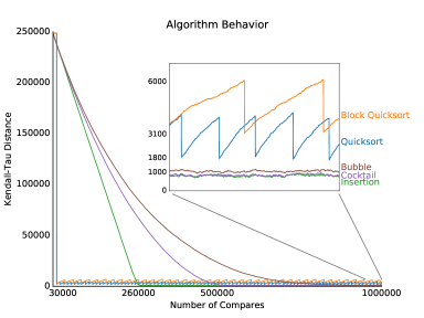
Figure 4: Impact of hotspot mutations. We plot Kendall tau distance as a function of an algorithm’s number of comparisons. We also show an enlargement of the tail-end steady behaviors.

A possible explanation for this behavior is that a large change in rank of a single element in a hot spot mutation can block a large number of other inversions from being fixed during a round of a quadratic algorithm. For example, in insertion sort, during a round, the element at each position, $0\leq i\leq n$, is expected to be moved to its correct position with respect to $0,\dots,i-1$ in $l$. To do so, an element $x$ is swapped left until it reaches a smaller element $y$. But if $y$ has mutated to become smaller, then all the elements left of $y$ in $l$, which remain larger than $x$, will stay inverted with respect to $x$ until the end of the round (unless some other mutation fixes some of them). Bubble and cocktail sort have a similar problem. An element $x$ which mutates can block other local, smaller inversions involving elements in between $x$’s starting and ending position. When these inversions are not be fixed, hot spot mutations make each pass of these algorithms coarser. Batch algorithms on the other hand are not affected as strongly by hot spot mutations, because their behavior depends on non-local factors such as pivot selection and the location at which the list was partitioned. Therefore, the movement of a single element has a smaller effect on their behavior. Thus, we find it even more surprising that the quadratic algorithms still beat the quicksort variants even for the hot spot adversary (albeit by a lesser degree than the amount they beat the quicksort variants for the uniform adversary).

3.6 Beneficial Swaps Performed by an Adversary

Note that our quadratic-time algorithms compare only adjacent elements, so they can only fix one inversion at each step. Therefore, they will not reach a steady state until the random swaps fix inversions almost as often as they introduce inversions. Figure 5 shows that the proportion of good swaps (those that fix inversions) to bad swaps (those that introduce inversions) approaches $1$ as $r$ increases. This behavior might be useful to exploit, therefore, in future work that would provide theoretical guarantees for the performance of bubble sort and cocktail sort in the evolving data model.

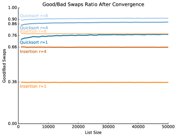
Figure 5: As $r$ increases, the number of inversions increases, but so does the number of beneficial mutations.

4 Conclusion

We have given an experimental evaluation of sorting in the evolving data model. Our experiments provide empirical evidence that, in this model, quadratic-time algorithms can be superior to algorithms that are otherwise faster in the traditional Knuthian model. We have also studied a number of additional questions regarding sorting in the evolving data model. Given the surprising nature of many of our results, it would be interesting in the future to empirically study algorithms for other problems besides sorting in the evolving data model. Alternatively, it would also be interesting to provide theoretical analyses for some of the experimental phenomena that we observed for sorting in the evolving data model, such as the performance of algorithms against the hot spot adversary.

A Detailed Convergence Behavior

In this appendix, we provide detailed convergence results.

In Table 1, we show specific convergence rates between insertion sort and quicksort, for a list of size 1000. As can be seen, this table highlights the expected result that quicksort reaches its steady behavior much more quickly than insertion sort. Thus, this table provides empirical evidence supporting a hybrid algorithm where one first performs a quicksort round and then repeatedly performs insertion sort rounds after that.

$r$	Insertion	Quicksort
0	500000	12000
1	510000	16000
2	513000	16000
3	516000	15000
4	516000	16000
5	521000	16000
6	523000	16000
7	521000	17000
8	525000	17000
9	524000	17000
10	527000	16000

Table 1: Number of comparisons needed to converge to steady behavior for different values of $r$.

In Table 2, we show the ratios of the number of inversions to list size for various values of $r$, with respect to the uniform adversary and multiple algorithms. Note that the ratios grow slowly as a function of $r$ and that the quadratic time algorithms are better than the quicksort variants for values of $r$ up to around 50. After that threshold, standard quicksort tends to perform better than the quadratic-time algorithms, but the quadratic-time algorithms nevertheless still converge and perform reasonably well. Interestingly, the quadratic algorithms still beat block sort even for these large values of $r$.

$r$	Insertion	Cocktail	Bubble	Quicksort	Block Quicksort
1	0.51	0.54	0.54	2.17	4.03
2	0.98	0.98	1.13	3.40	5.78
3	1.45	1.42	1.64	4.24	7.19
4	1.84	1.76	2.17	4.51	8.58
5	2.28	2.04	2.69	5.03	9.85
6	2.72	2.46	3.05	5.83	10.11
7	3.16	2.83	3.40	6.62	11.39
8	3.49	3.20	3.89	7.15	12.06
9	4.03	3.63	4.50	7.04	12.74
10	4.37	3.87	4.96	7.45	14.09
11	4.64	4.09	5.58	7.44	14.60
12	5.07	4.61	5.79	8.12	15.91
13	5.32	4.92	6.17	7.96	15.89
14	5.91	5.14	6.73	9.35	16.36
15	6.21	5.76	6.94	9.75	17.55
16	6.52	5.98	7.33	9.91	17.54
17	7.06	6.05	7.74	10.03	18.21
18	7.56	6.43	8.13	10.02	18.59
19	7.79	6.94	8.56	10.38	19.73
20	8.25	7.51	8.68	10.89	20.93
$\dots$
40	14.98	13.53	17.12	15.05	25.18
41	15.32	14.27	17.86	15.19	25.24
42	15.79	14.11	17.77	15.46	25.00
43	16.26	14.36	17.79	15.34	26.85
44	16.42	14.74	18.05	15.79	26.39
45	16.45	15.11	18.73	15.60	27.81
46	17.09	15.40	19.31	16.09	27.47
47	17.37	15.70	19.73	16.36	27.32
48	17.42	16.02	19.97	16.21	28.55
49	17.87	16.22	20.08	16.46	28.08
50	18.55	16.57	20.66	16.72	29.23
$\dots$
100	32.67	30.36	35.18	23.83	43.18
256	65.20	61.30	66.20	38.10	74.53

Table 2: Ratio of inversions relative to list size for different values of $r$

References

- [1] Aris Anagnostopoulos, Ravi Kumar, Mohammad Mahdian, and Eli Upfal. Sorting and selection on dynamic data. Theoretical Computer Science, 412(24):2564–2576, 2011. Special issue on selected papers from 36th International Colloquium on Automata, Languages and Programming (ICALP 2009). doi:http://dx.doi.org/10.1016/j.tcs.2010.10.003.
- [2] Aris Anagnostopoulos, Ravi Kumar, Mohammad Mahdian, Eli Upfal, and Fabio Vandin. Algorithms on evolving graphs. In 3rd ACM Innovations in Theoretical Computer Science Conference (ITCS), pages 149–160, 2012. doi:10.1145/2090236.2090249.
- [3] Bahman Bahmani, Ravi Kumar, Mohammad Mahdian, and Eli Upfal. Pagerank on an evolving graph. In 18th ACM SIGKDD International Conference on Knowledge Discovery and Data Mining (KDD), pages 24–32, 2012. doi:10.1145/2339530.2339539.
- [4] Thomas H. Cormen, Clifford Stein, Ronald L. Rivest, and Charles E. Leiserson. Introduction to Algorithms. McGraw-Hill Higher Education, 2nd edition, 2001.
- [5] Eleri Dixon, Emily Enos, and Scott Brodmerkle. A/B testing of a webpage, 2011. US Patent 7,975,000.
- [6] Mark E. Glickman. Parameter estimation in large dynamic paired comparison experiments. Journal of the Royal Statistical Society: Series C (Applied Statistics), 48(3):377–394, 1999. URL: http://dx.doi.org/10.1111/1467-9876.00159, doi:10.1111/1467-9876.00159.
- [7] Michael T. Goodrich and Roberto Tamassia. Algorithm Design and Applications. Wiley Publishing, 1st edition, 2014.
- [8] Qin Huang, Xingwu Liu, Xiaoming Sun, and Jialin Zhang. Partial sorting problem on evolving data. Algorithmica, pages 1–24, 2017. doi:10.1007/s00453-017-0295-3.
- [9] Varun Kanade, Nikos Leonardos, and Frédéric Magniez. Stable Matching with Evolving Preferences. In Klaus Jansen, Claire Mathieu, José D. P. Rolim, and Chris Umans, editors, Approximation, Randomization, and Combinatorial Optimization. Algorithms and Techniques (APPROX/RANDOM), volume 60 of LIPIcs, pages 36:1–36:13, Dagstuhl, Germany, 2016. Schloss Dagstuhl–Leibniz-Zentrum fuer Informatik. doi:10.4230/LIPIcs.APPROX-RANDOM.2016.36.
- [10] Maurice G Kendall. A new measure of rank correlation. Biometrika, 30(1/2):81–93, 1938.
- [11] Donald Ervin Knuth. The Art of Computer Programming: Sorting and Searching, volume 3. Pearson Education, 2nd edition, 1998.
- [12] Jialin Zhang and Qiang Li. Shortest paths on evolving graphs. In H. Nguyen and V. Snasel, editors, 5th Int. Conf. on Computational Social Networks (CSoNet), volume 9795 of Lecture Notes in Computer Science, pages 1–13, Berlin, Heidelberg, 2016. Springer. doi:10.1007/978-3-319-42345-6_1.