Response of an oscillatory delay differential equation to a periodic stimulus
Abstract
Periodic hematological diseases such as cyclical neutropenia or cyclical thrombocytopenia, with their characteristic oscillations of circulating neutrophils or platelets, may pose grave problems for patients. Likewise, periodically administered chemotherapy has the unintended side effect of establishing periodic fluctuations in circulating white cells, red cell precursors and/or platelets. These fluctuations, either spontaneous or induced, often have serious consequences for the patient (e.g. neutropenia, anemia, or thrombocytopenia respectively) which exogenously administered cytokines can partially correct. The question of when and how to administer these drugs is a difficult one for clinicians and not easily answered. In this paper we use a simple model consisting of a delay differential equation with a piecewise linear nonlinearity, that has a periodic solution, to model the effect of a periodic disease or periodic chemotherapy. We then examine the response of this toy model to both single and periodic perturbations, meant to mimic the drug administration, as a function of the drug dose and the duration and frequency of its administration to best determine how to avoid side effects.
keywords:
delay differential equation; periodic perturbation; delayed negative feedback; cycle length map; resetting time; blood cells; dynamical disease; cyclical neutropenia; cyclical thrombocytopenia;1 Introduction
Hematopoiesis is the term for the process of blood cell formation. Normally maintained at a homeostatic level within certain bounds (that vary between cell types), the numbers of circulating white cells, red cells, and platelets typically do not display any evidence of oscillatory dynamics. However, there are many hematopoietic diseases (so called periodic diseases [1]) in which cycling of one or more circulating blood cell types is seen. Examples include cyclical thrombocytopenia (CT) [2], cyclical neutropenia (CN) [3] and periodic chronic myelogenous leukemia (PCML) [4], and there have been numerous mathematical modeling studies of these disorders aimed at their understanding and treatment [5, 6, 7].
While cyclicity in circulating blood cell numbers is relatively rare in disease states, induced cyclicity of one or more circulating hematopoietic cell types as a byproduct of periodically administered chemotherapy is all too common. This cycling is most often encountered in the neutrophils (with a concomitant risk of infection when neutrophil numbers fall to sufficiently low levels), but also may be observed in the platelets (with an accompanying increased risk of bleeding and stroke at the low point of the platelet cycle, or thrombosis at the high point) as well as rarely in the erythrocytes (red blood cells, with accompanying anemia at the low point of the cycle). The commonality of this cycling with its attendant side effects (infection, bleeding, anemia) is one of the primary reasons leading to an interruption and/or cessation of chemotherapy.
In mammals hematopoiesis starts in the bone marrow with the proliferation and subsequent differentiation of hematopoietic stem cells (HSCs) into one of the three major cell lines, and ends with the release of mature blood cells into the circulation. Although all mature blood cells have the HSCs as their common origin, the control of their production is only partially understood [8]. However, the broad outline is clear.
The numbers of circulating blood cells are controlled by a delayed negative feedback mediated by cytokines, such as granulocyte colony-stimulating factor (G-CSF) for the white blood cells, thrombopoietin (TPO) for the platelets, and erythropoietin (EPO) for the red blood cells [9]. The periodic administration of chemotherapy, or the existence of hematological disorders like CN, PCML, or CT, may lead the level of peripheral blood cells to exhibit oscillations that are more or less regular [6, 7, 9]. There is a vast literature of mathematical models that propose how to control chemotherapy side effects or understand periodic hematological disorders, see for example Beuter et al. [8, Chapter 8], Foley and Mackey [7] and Pujo-Menjouet [10].
A scalar delay differential equation (DDE), with a linear piecewise constant negative feedback nonlinearity, which captures the essence of the negative delayed feedback mechanism involved in the control of blood cells by cytokines, was analyzed in Mackey et al. [9]. This equation has an oscillatory solution (to mimic an inherent oscillation due to a periodic disease or induced, for example, by the administration of chemotherapy), and was used as a toy model to examine analytically the effect of a single perturbation on the limit cycle. The single perturbation was applied at different points in the limit cycle to mimic the delivery of a cytokine (G-CSF, TPO, or EPO) and to examine the subsequent effect on the model oscillation. The single perturbation amplitude and duration were related to the dose and time of administration of an exogenous cytokine, as it is known that the timing of the administration of a cytokine can be crucial in its clinical effect [9]. In Mackey et al. [9] the results were limited to an examination of a single stimulus as the authors were unable to deal with the clinically more interesting case of a periodic stimulus. Here, we study the effect of a periodic perturbation on the dynamics of this delay differential equation.
This paper is organized as follows. Section 2 presents the model background and its DDE with discontinuous (Heaviside step function) delayed feedback and summarizes some fundamental results from Mackey et al. [9] concerning the response of the limit cycle to a single stimulus. Section 3 extends the analysis from Mackey et al. [9] of the response of the periodic solution to a single stimulus. We further define the concept of resetting time for a single perturbation and investigate its maximum and minimum values as function of the perturbation phase. We also describe a special case where changes in the phase and amplitude of the perturbation leads to solutions close to unstable limit cycles.
Section 4 analyzes the response of the DDE to a periodic perturbation. We define sufficient conditions to obtain a periodic solution such that all local minima are positive (clinically important), and also show examples of solutions with different numbers of local minima and maxima. The proofs of all the results stated in the remarks and propositions are presented in Appendix A. Section 5 considers our modeling results in the context of cytokine administration, and carries out a detailed comparison with a more comprehensive model of [11]. The penultimate Section 6 presents a variety of bifurcation results in our model system, while Section 7 gives a brief summary and prospects for further work.
2 Model Background
Here we consider the simple mathematical model used in Mackey et al. [9] to describe the dynamics of a circulating blood cell population in which the cell death rate of circulating cells is denoted by and their production rate is described by a delayed negative feedback mechanism . The delay captures the physiologically known delay due to cellular division, differentiation and maturation. The dynamics of is taken to be described by (see Mackey et al. [9])
| (1) |
where the piecewise constant nonlinearity is of the form
| (2) |
with , , , . To solve the initial value problem (1) we must specify the initial function
| (3) |
Denote the solution of (1) with initial function (3) by and the zeros of the solution for as the set of all , with , such that . Here we only consider initial (history) functions (3) that are continuous with a finite number of zeros. Denote by a set of history functions which has at most one zero on and changes sign at this zero. Given a history function , it follows from Mackey et al. [9, Section 3] that has a strictly increasing sequence of zeros in , , such that
The model given by (1) and (2) contains five parameters . Using the change of variables
| (4) |
we can rewrite (1)-(2) as a function of three parameters , namely
| (5) |
where
| (6) |
with , . Eq. (5) with defined by (6) captures the negative delayed feedback mechanism involved in the control of hematopoietic cells by cytokines. For the initial function
the solution of Eq. (5) is a limit cycle , and is given by (7) [9] and is presented in Figure 1.
| (7) |
where the minimum and maximum of are given by [9]
| (8) |
is the period of the limit cycle (7) and , with represents the zeros of . For we have . The period and the zeros , are given by (9) [9].
| (9) |
At where the limit cycle has a minimum point and at the maximum of the limit cycle when the derivative of is undefined. From (9) it is clear that for all .
For every history function restricted to the set the solution of (5)-(6) converges to the limit cycle (7) within a finite time and with a new phase, and this limit cycle is stable [9, Theorem 3.3]. The DDE (5)-(6) admits infinitely many other periodic orbits, but are all unstable [9, Remark 3.2 and 3.3].
3 Single Stimulus
In this section we consider the response of Eq. (5) to a single pulse perturbation. We summarize some notation from Mackey et al. [9], defining the resetting time for the pulse-like perturbation and distinguishing it from the concept of cycle length map defined in Mackey et al. [9]. We show that the resetting time is always less than the cycle length map, and that the minimum resetting time is equal to or greater than the stimulus duration. We also show how a single perturbation can lead to an infinite resetting time because of an unstable limit cycle. The influence of the amplitude, phase and time duration of the perturbation on the cycle length map is also examined.
Consider a single pulse-like perturbation of amplitude and duration which starts at , where is the period of the periodic solution of Eq. (5) with given by the discontinuous function (6). For Eq. (5) becomes
| (10) |
Mackey et al. [9] examined the response of the limit cycle (7) to a single pulse-like stimulus with positive amplitude , as defined in Eq. (10). They calculated the minima, maxima and period of the perturbed limit cycle for different values of the starting time and duration of the single pulse-like perturbation. (The single stimulus of amplitude and duration can be related to the dose and temporal duration of the administration of exogenous cytokines in an attempt to regulate the peripheral blood cells [9]).
The response of the limit cycle solution (7) to a perturbation with amplitude can be calculated piecewise by considering the phase which the stimulus begins and ends . We distinguish the perturbation for different values of as in Mackey et al. [9].
To use the same notation, we classify the stimulus distinguishing whether it begins in a rising phase R (), falling phase F (), with negative value N (), or non-negative value P (); and whether it ends in a phase R or F, with value N or P. Precisely, including the points where the derivative is undefined, we use the nomenclature R for , F for , P for , and N for . For example, the sequence of letters RPFN denotes a pulse which begins in the rising phase with positive value and ends in a falling phase with negative value. We also denote the solution of the DDE with perturbation (10) by , and its zeros by , with , as in Mackey et al. [9]. The zeros of form an increasing sequence with [9]. With this classification we have the following sequence of possibilities [9]:
| (11) |
Each subcase (11) is defined on a -subinterval . For each parameter vector there is a set of subcases (11). The union of all their -subintervals is equal to and their intersection is the empty set. We denote the -subintervals as with a subscript with the respective sequence of letters, e.g. for the case RNRN the -subinterval is denoted by .
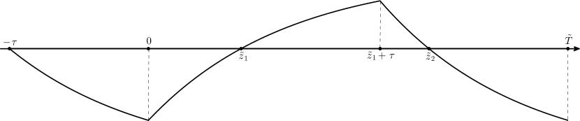
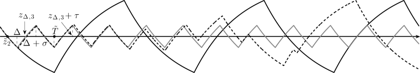
For the subcase FNFP, the time required for the perturbed solution to return to the limit cycle may not be finite everywhere due to a rapidly oscillating periodic solution [9]. This is the most complex case in (11) and will be analyzed here in detail. In this case the pulse starts in the falling phase of the limit cycle with , which implies . The pulse also ends in the falling phase, i.e. , and with positive value . The positivity condition implies , where is a constant defined by , which yields
| (12) |
the same constant defined in Mackey et al. [9, Eq. (5.11)]. Thus the -subinterval in the case FNFP is of the form
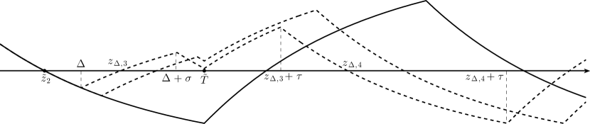
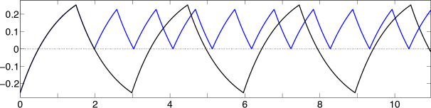
In Remark 3.1 we show that the inequality holds for the case FNFP and we distinguish between two subcases, FNFP1 and FNFP2. For the case FNFP1 we have as in the perturbed solutions shown in Figure 2, while for the case FNFP2 we have as in the examples displayed in Figure 3.
Remark 3.1.
The inequality holds for the case FNFP and we can distinguish two subcases by incorporating further conditions as follows:
-
1.
FNFP1 If , then
(13) -
2.
FNFP2 If , then
(14)
where the constant is such that for and is given by
| (15) |
(Remember that all proofs are presented in Appendix A.)
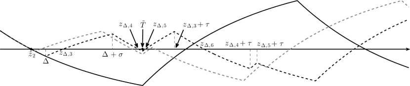
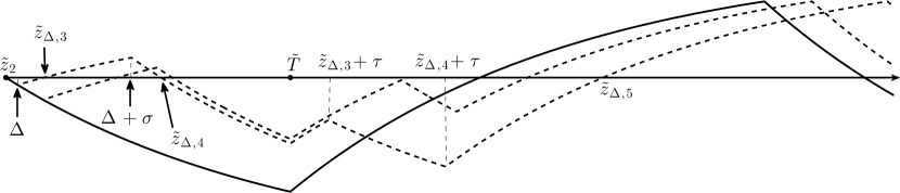
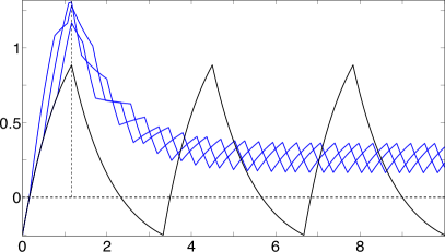
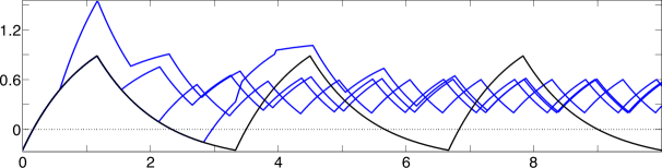
In Remark 3.2 we show that the case FNFP2 from Remark 3.1 can be distinguished between two subcases by including the extra condition to define the case FNFP3, and the extra conditions and to define FNFP4. The examples of solutions shown in Figure 3 correspond to the subcase FNFP2 and also FNFP4 while the examples of solutions shown in Figure 4 refers to case FNFP3. The case FNFP2 actually splits into an infinite number of subcases, and examples are shown in Figure 5. The solution represented by the dashed line in Figure 5 shows how long the transient solution can be before it returns to the periodic orbit.
Remark 3.2.
Between the case shown in Figure 3 and the rapid limit cycle shown in Figure 5 there is a sequence of subcases. For each new case the solution oscillates one more time before approaching the limit cycle. For all solutions of the cases FNFP it is expected that .
For a perturbation with starting time we define the resetting time as the time interval required for the perturbed solution to return to the limit cycle with a new phase. We formally define the resetting time in Definition 3.1 and give it for each case (11) in Remark 3.3.
Definition 3.1.
Resetting time. Let us define the function . Assume that the limit cycle is perturbed at time , as in (10), and that after a time interval , defined as the resetting time, the perturbed solution returns to the limit cycle with a new phase and stays on it, i.e. holds for all .
Remark 3.3.
By definition, the resetting time is the minimum time required for the perturbed solution to return to the limit cycle, while the cycle length map is the time measured between two marker events [1], one located before the solution is perturbed and the other after the perturbed solution has returned to the limit cycle. The cycle length map is given by , where is the phase difference between the two marker events. In Mackey et al. [9] the zeros of the limit cycle, , and the zeros of the perturbed solution, , were used as marker events to calculate the cycle length map . Thus, by definition, the resetting time is always less than the cycle length map, c.f. Remark 3.4.
Remark 3.4.
For all with () we have .
In the next section we consider (10) with a periodic perturbation instead of a single perturbation. Thus it will be of interest to know whether and are finite, and to know their lower and upper bounds. We define the maximum and minimum of the resetting time and cycle length map respectively by
As expected, for all and the minimum resetting time is equal to or greater than the stimulus duration , as detailed in Remark 3.5. In Remark 3.7 the maximum of for the case is investigated.
Remark 3.5.
For all and with () we have .
Remark 3.6.
For the inequality holds and .
Remark 3.7.
For the maximum of the cycle length map occurs at and is given by
| (18) |
Remark 3.6, and the fact that the cycle length map is continuous for [9, Corollary 4.2], allows us to compute a maximum of as stated in Remark 3.7.
As consequence of Remarks 3.4 and 3.5, is a lower bound for the cycle length map, i.e. . From Remarks 3.7 and 3.4 it follows that for the maximum (18) is an upper bound for the resetting time, i.e. .
For the resetting time and cycle length map may not be bounded above. For all of the cases in (11) the case FNFP is the only one in which the cycle length map may not be finite everywhere [9]. In Figure 5 we show perturbed solutions that illustrate how a single perturbation to FNFP can lead to an infinite resetting time due an unstable limit cycle. In Remark 3.8 we show that for equal to (19) the perturbed solution settles down on a rapidly oscillating unstable periodic solution with whose period satisfies .
Remark 3.8.
For the case FNFP the cycle length map and the resetting time both tend to infinity when tends to the constant which is given by
| (19) |
and satisfies . For the perturbed solution settles down on a rapidly oscillating unstable periodic solution for which the period satisfies and is given by . Moreover, the minimum and maximum of the rapid limit cycle are given by
and satisfy and .
Next we investigate how the cycle length map computed in Mackey et al. [9] varies with changes in the perturbation amplitude and the pulse duration .
Figures 6(a) and (c) show how changes as function of , while panels (b) and (d) show how changes when is varied. For all examples of the four panels . All curves of panel (a) are continuous on . In panels (b) and (d) we see that for a Type 1 discontinuity [12] appears in the cycle length map. All curves show this discontinuity in panel (c). In the limit we have , , and . The decreasing length of both intervals and as is decreased can be seen by comparing the curves with from panels (b) and (d). For panel (b) while for panel (d) and the intervals and approach vertical lines for and , respectively.
In Figure 6 the intersections points where are so-called fixed points of the cycle length map and they are unstable if and stable if [13], where denotes the derivative of with respect to evaluated at .
For the cycle length map is continuous [9, Corollary 4.2]. Figure 7 shows the cycle length map and time resetting for the examples with dark blue lines from Figure 6(a) and (b). In panel (a) we have , is continuous and the vertical dashed lines indicate the points where is discontinuous. From left to right the lines respectively correspond to equal to: , and . The graphs correspond to the following sequence of cases: RNRP, RPRP, RPFP, RPFN, FPFN, FNFN, FNRN, FNRP. In panel (b) we have , has a discontinuity at and the vertical dashed lines indicate the points where is discontinuous. From left to right the lines are respectively given by equal to: , and . For this example we have the following sequence of cases: RNRP, RPRP, RPFP, FPFP, FPFN, FNFN, FNRN, FNRP.
In the examples from both panels of Figure 7 we have , . Thus the discontinuity of at in Figure 7(b) is due to how the cycle length map is defined and not due to the dynamics. This type of discontinuity is called Type 1 [12]. On the other hand, the resetting time presents three discontinuities on each panel of Figure 7 and independently of the way that is defined, it has two discontinuities which are defined as Type 0 [12].
4 Phase Response to a Periodic Stimulus
In a clinical setting, it is more likely that a patient would receive periodic administrations of a cytokine to ameliorate the effects of periodic chemotherapy. However, there has been controversy about how to best time these administrations.
Here we examine the response of the DDE (5) to a periodic perturbation . We keep , , and . The perturbation is ON during a time interval and OFF during a time interval , so the period is . The perturbation is defined by
| (20) |
where , and .
We denote the solution of the perturbed DDE by which, up to , is equal to the periodic solution . For the function is defined by
| (21) |
with and given by (6) and (20), respectively. The solution of (21) is built up piecewise by functions of the form for each interval with and , where are the points where the derivative is discontinuous. These discontinuity points are known as breaking points in the literature [14]. Along the solutions of (21) the breaking points are located at the points where switches from a negative to non-negative value or switches from positive to zero. Thus for the solution of (21), , is given by
In order to examine the effect of the periodic stimulus we will consider the perturbation period and resetting time due to each perturbation. Recall that by definition and from Remark 3.5 we have for all , then . The analysis of the periodic perturbation must distinguish between two cases, and .
Case (i) . After each perturbation the solution returns to the periodic solution , with a new phase, before the next perturbation starts. Hence, in this case the solution can be computed on each interval and , with , as was done in Mackey et al. [9, Section 5]. For the special case where and the solution is periodic. For this singular case the time interval that the solution takes to return to the limit cycle is equal to the perturbation period and is such that the solution returns to at the same phase that it had when it left the limit cycle. For the cases where or and the solution may become periodic after a finite number of stimuli or may continue to be non-periodic.
Case (ii) . For this case the solution will be periodic if . Again for the special case where and the solution is periodic, but here , as is shown in the example of Figure 8. For the cases where or and , after the end of the first perturbation, , the next perturbation may start before or after the perturbed solution returns to the limit cycle. In both cases the second stimulus will not start at the same phase of the limit cycle where the first stimulus started. Thus, each perturbation starts with a different phase, with respect to the previous, and it may occur that the phases repeat after a finite number of stimuli, resulting in a periodic solution. Otherwise, the phases will not repeat during successive perturbations and the solution may be quasi-periodic or non-periodic.
The numerical solutions of Figure 8 and onwards were computed using the MATLAB dde23 routine [15]. All solutions of (21) are composed of piece-wise function segments on intervals , where are the breaking points. These breaking points were detected and included in the solution meshes by using the MATLAB events function [15, 16].
In Proposition 4.1 below we show that if and , then the solution converges to the orbit given by (23) and (24).
Proposition 4.1.
In Proposition 4.2 we show that the solution of Proposition 4.1 converges to a limit cycle. We compute this periodic solution and show that if the phase of the first perturbation overlaps with the minimum point of the limit cycle, then the perturbed solution settles down on this limit cycle.
Proposition 4.2.
If , then: (i) the solution of (21) converges to the limit cycle given by (27), (ii) for and a non-negative history function , with , and such that , the solution of (21) settles down on the limit cycle given by
| (27) |
for , where and are defined by
| (28) |
| (29) |
In Propositions 4.1 and 4.2 it is shown that the perturbed solution converges to a limit cycle if and . For we have and .
For or and the long-time behavior of the solutions for both Cases (i)-(ii) described earlier does not depend on the value of . Indeed, the results of Propositions 4.1 can be extended for all , which was done in Proposition 4.3. Figure 9 shows examples of solutions, distinguishing four cases, which satisfy the conditions of Proposition 4.3. All solutions of Figure 9 converge to a limit cycle given by (27). In panel (b) and (c) the solution points and exponentially converge to (28) and (29), respectively. In panel (a) this convergence occurs for while for panel (d) it occurs for , where is the first zero of with .
5 Treatment Implications
At this point it is interesting to consider our results with this extremely simple model in the context of a hypothetical patient with cyclic circulating blood cell numbers (e.g. cyclic neutropenia, or cycling induced by chemotherapy) being treated with periodic G-CSF administration. We denote the normal level of neutrophils by . For cyclic neutropenia the circulating neutrophil numbers typically oscillate from normal levels to very low levels with a period of about 19 to 21 days [3]. The period for cycling induced by periodic chemotherapy is approximately equal to the period of the chemotherapy [5].
One issue of interest is whether or not it is possible to abrogate the severe neutropenic phases of the oscillation in the model as is done in practice by keeping the circulating neutrophil levels equal to or greater than normal. We can answer this in the affirmative, since the condition is sufficient to end the neutropenia. Using (22) and (28), the condition to end the neutropenia can be written as
| (30) |
From (30) we obtain the condition , which satisfies the condition from Proposition 4.1 and increases the nadir of the oscillations to, or above, the normal level .
During the periodic G-CSF administration the hypothetical patient will have a neutrophil oscillation described by a limit cycle given by Proposition 4.2 with an oscillation amplitude given by
Notice that and we only have for , or , or .
To avoid neutropenia, in the limiting case we can force in (30), which gives . This satisfies the condition from Proposition 4.1 and in combination with (22) yield the minimal interval between administrations to avoid neutropenia as function of the duration and the amplitude of cytokine administration:
| (31) |
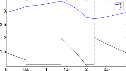
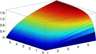
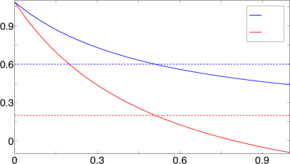
In Figure 10(a) we show that for the minimal interval between cytokine administrations to avoid neutropenia, given by (31), increases as the duration and/or the amplitude of the cytokine dose increase. In panel (b) we show that the minimum , given by (28), is decreasing with respect to the time interval between cytokine administration and increasing with respect to the duration of the administration. Both effects are what one would intuitively expect.
We also investigate the hypothetical situation where the periodic G-CSF administration still results in neutropenia and the neutrophils oscillate between and where . We mimic this situation by imposing the conditions
| (32) |
For a healthy adult human the normal circulating neutrophil level fluctuates around of body mass [5]. Assuming that we want to administer G-CSF to maintain the oscillation within these normal bounds and taking , then we have and . In order to solve (32) we need to fix one of the triplet and then solve for the remaining two parameters.
Both limit cycle extrema and are nonlinear increasing functions with respect to , nonlinear decreasing functions with respect to , and linearly increasing with respect to . Thus we take and as unknowns and solve (32) with the set of parameters: , , and , , and . Using the MATLAB fsolve routine [15] to solve (32) gives and .
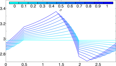
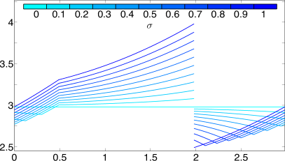
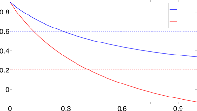
In Figure 11 all the four solutions with different initial perturbation phases converge to the same limit cycle, which is given by Proposition 4.2, but with different phases. We also investigated how and change as function of in Figure 12(a) and (c) and as function of in Figure 12(b) and (d) considering the same parameters of Figure 11 in panel (a) and (b), but with in panel (c) and in panel (d). We have and for in panel (a) and for in panel (b). In both panels (c) and (d) there is a parameter interval such that and are bounded above by and bounded below by .
Several mathematical models have used a DDE similar to (5)-(6) to study blood cell dynamics, but with different feedback functions (6), and it would be of interest to know how our results compare with those obtained in more complicated (and physiologically more realistic) treatments. One could think of, for example, the Hearn et al. [17] model for canine cyclical neutropenia, or the neutrophil models of Zhuge et al. [11] and Brooks et al. [18] which consider GCS-F administration during chemotherapy in humans.
Here we consider the neutrophil model from Zhuge et al. [11]. Equation (2) from Zhuge et al. [11] describes the dynamics of bone marrow hematopoietic stem cells and circulating neutrophils . We decouple the neutrophil dynamics from the stem cell dynamics by assuming that stem cells are at their normal steady state concentration of body mass. Thus the second component of equation (2) from Zhuge et al. [11] becomes
| (33) |
where is the neutrophil apoptosis rate, is the amplification factor, is the rate that stem cells commit to differentiate to neutrophil precursors, and is the total time it takes to a neutrophil be produced which is defined as the sum of the neutrophil proliferation time and the neutrophil maturation time , i.e. [11]. The neutrophil proliferation phase duration is constant and equal to , while the neutrophil maturation phase duration depends of the G-CSF serum level. We consider that for a G-CSF dose of the neutrophil maturation time is equal to , as estimated by Zhuge et al. [11]. The normal level of circulating neutrophils is taken to be of body mass [11].
Assuming periodic administration of G-CSF the amplification can be expressed as , where and is the periodic perturbation due to the G-CSF [11]. Without G-CSF the amplification factor is constant and equal to [11]. We can rewrite (33) as
| (34) |
where is the delayed negative feedback, is a periodic perturbation assumed to be of the type (20), but with , and in units of days and in units of . As in Zhuge et al. [11], we consider that the effects of G-CSF are maintained for one day and that the interval between consecutive administrations is also one day . We approximate the delayed negative feedback by the piecewise constant function
| (35) |
and take equal to the feedback maximum value , where [11], and with . The change of variables , , , , followed by the change of variables (4) together with transform Eq. (34) with given by (35) into the form (21). Taking and the parameter values earlier described we compute the parameters from (21) as being , , , and , where and are in units of of body mass.
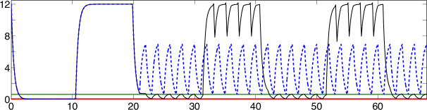
For this set of parameters, oscillates between and with a period of days as shown in the first day portion of Figure 13 where we plot , where and is the solution of (21). The remainder of Figure 13 for days to shows the simulated effects of G-CSF treatments for two different perturbation amplitudes. The black line corresponds to a G-CSF dose of while for the blue line . Both perturbations start at day 21, i.e. . The green line corresponds to the normal neutrophil concentration while the red line is the reference level for severe neutropenia, namely 111Human neutropenia is classified as severe if the neutrophil concentration is below (of body mass), which corresponds to an absolute neutrophil count (ANC) of [6]. For the black line the perturbation amplitude is such that the neutrophil concentrations are greater than or equal to the reference level for severe neutropenia, while for the blue line the amplitude is such that the neutrophil concentrations are equal to or greater than the normal level . For the black line has a maximum value of about (of body mass) which is slightly larger than the maximum value reached without perturbation.
In order to compare the effects of the same G-CSF perturbation in both models, we estimate the amplitude of perturbation from (34) through the negative feedback function from (33) by computing its variation for the value of under the G-CSF effects and without the effects of G-CSF . Under the effects of a G-CSF dose of the amplification rate can be approximated by , where is the neutrophil maximal proliferation rate, is the neutrophil minimal death rate in maturation, and is the maturation time, yielding the figure [11]. This figure together with the change of variables gives the approximation for perturbation amplitude of body mass. For this amplitude and considering the other parameters as are in Figure 13, the dynamics of neutrophil concentration (not shown) is similar to the behaviour observed for the blue line from Figure 13, it cycles with the same period of the G-CSF administration, but with varying from to of body mass. This variation is much larger than the oscillation due to the G-CSF administration obtained in Zhuge et al. [11], see the first few days of the simulation with red line presented by the authors in Figure 3(b). This perturbation amplitude value also is about 30-fold larger than the amplitude necessary to end neutropenia considered for the simulation with blue line shown in Figure 13.
The discrepancy in the response of both models to the same perturbation amplitude is related with the difference between their negative feedback functions, but it also might be related with the fact and that the response to G-CSF is highly variable for the model from Zhuge et al. [11], as indicated by the authors.
Consider the limit cycle shown in Figure 13 for , where and is the solution of (21), the perturbation amplitude is zero and the other parameters are as in Figure 13. Define the minimum, maximum and period of oscillation for respectively by , and , where , and are given by (8) and (9). This together with and , where , yields (of body mass), (of body mass) and . The choice of values for and from the feedback function (35) defines the parameters and and therefore it is important to define the minimum and maximum of the oscillation, since and , but it does not play an important role for defining the oscillation period. Indeed, increases linearly with the delay and for varying from to the period stays between and , which are close to the periods of observed for CN [3].
For a wide range of values of the parameters , (and so , ) the solution of Eq. (34) with given by (35) yields a neutrophil dynamics characteristic of CN, with periods close to and minimum and maximum of the oscillation given approximately by and , respectively. So the piecewise linear feedback function (35) may be used as reference to construct nonlinear continuous feedback functions such as those from the mathematical models Zhuge et al. [11] and Brooks et al. [18] in order to model CN dynamics, namely the period, maximum and minimum of the oscillations.
Daily administrations of G-CSF in both humans and grey collies with CN has the effect of reducing the oscillation period and increasing both the neutrophil nadir and the oscillation amplitude [17, 3]. For the model (34) with given by (35) the G-CSF perturbation does increase the neutrophil nadir, as shown in Figure 13 simulations. However, for the simulation with black line shown in Figure 13 the oscillation amplitude is only slightly increased and the period stays close to the period of oscillation, while for the simulation with blue line both the amplitude and period of oscillation decreases. These results indicates that the perturbation from (34) does not capture the G-CSF effects on either the period and amplitude from CN oscillations. Thus we must conclude that the simple model considered here deviates considerably from the supposedly more physiologically realistic model of [11]. While disappointing it is hardly surprising considering the differences in the two models.
We can also compare the model effects of periodic administration of chemotherapy for a healthy human by reducing Eq. (34) with given by (35) into the form (21). So the neutrophil dynamics is given by , where and is the solution of (21). For this onset of chemotherapy the amplitude of the periodic perturbation must be negative (only for this onset we assume that ). We simulate the situation where a normal human receives chemotherapy doses with period of administration varying from 1 to 40 days, as is considered in Zhuge et al. [11].
As mentioned earlier, for a healthy adult human the normal circulating neutrophil level fluctuates around of body mass. These levels are similar to the neutrophil concentrations shown in Figure 2(b) of Zhuge et al. [11] for the first few days, before the chemotherapy begins. Thus, before chemotherapy we have and we obtain that the neutrophil concentration is a limit cycle which oscillates from to by taking , , and the other parameters as in Figure 13, with , , and in units of of body mass. For this set of parameters the period of oscillation is .
As in Zhuge et al. [11], we consider that the effects of chemotherapy is maintained for one day, so . We compute the amplitude of perturbation by considering that for a daily administration of chemotherapy the neutrophil nadir is zero, i.e. , from where it follows that
| (36) |
For this set of parameters the neutrophil concentration was numerically computed for for each period of administration , where with and fixed at . For each period Figure 14 shows the amplitude and nadir with for panel (a) and for panel (b). For all simulations the first perturbation begins at zero and the history function of (21) is given by
| (37) |
which is equivalent to the segment of the limit cycle (7) for . For the solution of (21) is given by
| (38) |
The first perturbation begins at . So at the end of the first perturbation we have and (38) yields
| (39) |
| (40) |
The history function (37) considered here gives the shortest nadir possible for at the end of the first perturbation. Although we have not proved this results mathematically, it is intuitive that for the scenario of a single perturbation and considering the history function (37), the minimal value of the solution (21) as function of the phase occurs for and at the end of the perturbation (). This minimal value is given by (39) and the correspondent neutrophil minimal level is given by (40).
In Figure 14(b) the neutrophil nadir converges to the minimal level (40). For the neutrophil minimum levels after the transient dynamics is smaller than and the nadir increases with . For the time interval for which the perturbation is turned off is large enough for the perturbed solution (21) returns to the unperturbed limit cycle (7) before the perturbation be turned on again. Thus for the minimum levels of neutrophil only depends on which phases of the unperturbed limit cycle (7) the perturbation is turned on and the resulting nadir is approximately equal to (40).
The amplitude and nadir curves shown in Figure 14(b) are essentially the same when they are computed for instead of . Comparing the nadir values and amplitude values for both time intervals and the same mesh , their maximum absolute difference is smaller than of body mass.
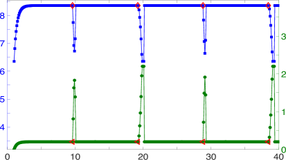
In Figure 14(a) the triangular symbols indicate the nadir for the points with and show that they are close to the nadir resonance peaks. For the first resonance peak the maximum occurs for days and for the third peak it occurs for days. The second and fourth resonance peaks are limited above by the nadir of the unperturbed limit cycle of body mass. Their maximum values stay constant at along the three points , and days for the third resonance peak, and along the four points , , and days for the fourth peak.
The results shown in Figure 14(a) are quantitatively and qualitatively different from the results shown in Figure 2(a) from Zhuge et al. [11]. In Figure 2(a) from Zhuge et al. [11] the nadir and amplitude vary considerably along the interval , and at the resonance points the amplitude increases and the nadir decreases. While in Figure 14(a) the nadir and amplitude increase rapidly for and are essentially constant for , except at the 4 narrow resonance peaks, where the amplitude decreases and the nadir increases substantially.
Administration protocols of common chemotherapeutic drugs (such as docetaxel, cyclophosphamide, cisplatin, paclitaxel, etc.) often prescribe a chemotherapy cycle of three weeks [11]. Our simulations in the current model would suggest that chemotherapy treatments with cycles close to 21 days do not affect the nadir levels, except that for cycles inside of the narrow interval from about 19.9 to 20.1 days would increase the neutrophil nadir along the treatment.
So, again, the results of the simple model considered in this paper seem to be at odds with the results of the model of [11].
6 Bifurcations in the Face of Periodic Perturbation
Periodic perturbation can give rise to periodic solutions through a variety of bifurcations, and in this section we explore these. We examined these mechanisms and how the local maxima and minima of the solution change by performing one parameter continuation on the extremal points.
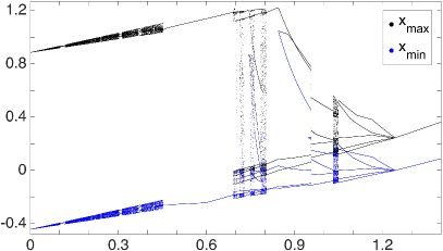
In Figure 15 we present orbit diagrams for (21) as one of each of the parameters is varied. Orbit diagrams are normally produced for maps, but we can reduce the solution of (21) to a map by considering crossings of a Poincaré section which contains the local maxima and minima of along the solution [19].
All graphs of Figure 15 were constructed with the following technique. A mesh with points was used to compute the solutions for increasing parameter values (noted on each abscissa) for panels (a) and (c) and for decreasing parameter values for panels (b) and (d). For all mesh points the orbits were computed using the MATLAB dde23 routine [15], with an absolute error of and relative error of . The points where the trajectory is discontinuous were detected and included in the solution mesh by using the MATLAB events function. For each mesh point we integrated through a transient of , and then plotted all the maxima and minima that occur over the next . The last time units of the solution is used as the history function to compute the solution at the next mesh point. We also used the function Jumps of the MATLAB dde23 routine to include the discontinuity points in each history function mesh to compute the solution of the next mesh point. For the first mesh point we integrated through a transient of length .
In all panels of Figure 15, the one parameter continuation reveals numerous points of period-doubling bifurcation of periodic orbits and several parameter intervals of periodic dynamics and windows of irregular motion. Panels (a) and (b) respectively show that the smallest minima of the solutions increases, except for small variations, as the perturbation amplitude or the time duration of perturbation are increased. Conversely, panels (c) and (d) respectively show that the smallest minima of the solutions decreases, except for small variations, as or the delay are increased.
Figure 15(a) shows discontinuities in the extrema for , while panel (b) shows discontinuities for and . These discontinuities are due to numerical issues and must disappear by increasing the integration time and the mesh size. However, it was verified that doubling the the integration time and/or the mesh size was not enough to remove these discontinuities. While it would be interesting to obtain these graphs with continuous extrema, it might take a long time to find a suitable integration time and mesh size because every attempt requires to solve the DDE (21) numerically with a reasonable precision and also include the breaking points in the solution meshes. We have not pursued this issue in this paper.
In the left side of Figure 15(c) we see a parameter interval with a simple limit cycle followed by intervals with period-5, -4 and -3 limit cycles, where the period-3 region ends with an abrupt transition to irregular motion. A small parameter change can thus cause periodic motion to become irregular, and vice versa.
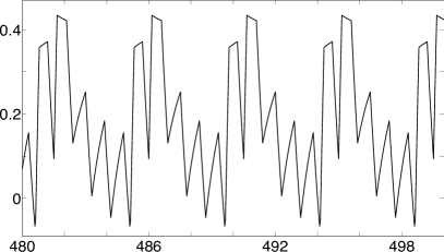
Figure 16 shows a period-5 limit cycle in panels (a)-(b), a period-8 limit cycle in panels (c)-(d) and a complex solution in panels (e)-(f). For all three orbits we used and we have and . Orbits from Figure 16(a)-(b) correspond to solutions of Figure 15(a) for and orbits from Figure 16(c)-(d) are related with solutions of Figure 15(c) for . The solutions shown in Figure 16(e)-(f) correspond to solutions with inside of the windows of apparent chaotic dynamics of Figure 15(d).
For some parameters , there can occur frequency locking between the perturbation period and the limit cycle period . For example, for the limit cycle shown in Figure 16(a)-(b) we have and which yields a frequency locking 5:1, while for the solution of Figure 16(c)-(d) we have and , with a frequency locking of 29:1. The solutions shown in Figures 9 and 11 converge to limit cycles where , and a frequency locking of 1:1. In fact, the frequency locking 1:1 occurs for all limit cycles with (see Proposition 4.2 and 4.3).
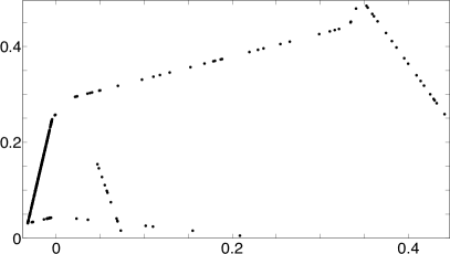
In order to solve (21) it is necessary to define a history function for , which is an infinite-dimensional set of initial conditions. Thereby the solution space of (21) is infinite dimensional and consequently a hyperplane defined by a Poincaré section is also infinite dimensional. Although the Poincaré section is infinite dimensional, we can project it onto by taking, for example, the solution points and such that for some constant . In Figure 17 we project a Poincaré section of the orbit of Figure 16(e)-(f) onto the plane for crossing of the Poincaré section with for panel (a) and for panel (b). Both Poincaré sections form a locus with sparse points, indicating that the irregular motion of the orbit of Figure 16(e)-(f) is chaotic [20].
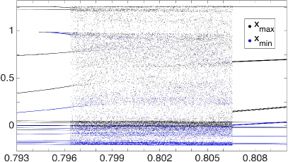
Figure 18(a) shows a magnified part of the diagram of Figure 15(c). In the other panels we show orbits from the diagram of panel (a) transitioning from a region of regular motion to regular motion. In panel (a) we have an irregular motion with , in panel (b) we have and the orbit changes from irregular to regular motion for , while in panel (c) the transition to regular motion occurs for . This scenario of an abrupt transition from periodic motion to irregular motion and vice versa is highly suggestive of a boundary or an exterior crisis scenario [20, 21].
7 Discussion and Conclusions
Here we have been able to exploit the relative simplicity (due to the piecewise linear nonlinearity) of our model system in an extension of the results of Mackey et al. [9] examining the response to a single stimulus (Section 3), as well as examining the response of the system to a periodic stimulus in Section 4. The insights and techniques of Section 4 allowed us to draw conclusions about treatment implications in Section 5. The numerical bifurcation diagrams of Figure 15 revealed that an effective way to increase the minima of the oscillations, and hence decrease the neutropenia duration, is to increase the drug dosage by either increasing the time duration of the drug administration , or increasing the drug dose administrated per unit of time, which is proportional to . From Propositions 4.1 and 4.2 and Eq. (31) we obtained the condition to avoid neutropenia, from which we computed the minimal interval between drug administrations to avoid neutropenia as function of the time duration of the drug administration by Eq. (31).
The numerical results we have presented in Section 6, while not exhaustive, certainly indicate that there is a wealth of bifurcation behaviour to be understood in this relatively simple system. However, this must remain the object of further study as it is outside the main thrust of this paper.
Finally we note that the study of periodic perturbation of limit cycle systems has been long and intensive, particularly in a biological context, c.f. Winfree [12], Guevara and Glass [22], Glass and Winfree [23], Krogh-Madsen et al. [24], Bodnar et al. [25], and the emphasis has been on an examination of the phase response curve. However, to apply numerical methods such as the phase reduction method due to Novicenko and Pyragas [26] and Kotani et al. [27] to calculate the phase response (or phase resetting) curve for a DDE and the method to compute the approximating Lyapunov exponents for DDEs due to Breda and Van Vleck [28] we need to linearize the DDE (21) around a reference orbit, but the feedback function is discontinuous at . An extended approach using (21) with a continuous delayed feedback (a sigmoid type) would allow us to apply these numerical methods to study the solutions with approaching the discontinuous delayed feedback. This too we reserve for a future study.
Acknowledgments
DCS was supported by National Council for Scientific and Technological Development of Brazil (CNPq) postdoctoral fellowship 201105/2014-4, and MCM is supported by a Discovery Grant from the Natural Sciences and Engineering Research Council (NSERC) of Canada. MCM would like to thank the Institut für Theoretische Neurophysik, Universität Bremen for their hospitality during the time in which much of the writing of this paper took place. We are very grateful to Tony Humphries for fruitful discussions and suggestions.
Appendix A Proof of the Results
Proof of Remark 3.1.
First it is shown that holds. For we have
| (41) |
with and
| (42) | |||||
| (43) |
From (42) the condition can be written as
but since , then we must have .
For we have
| (44) |
Proof of Remark 3.2.
FNFP3: for this subcase we have to assume (see the examples in Figure 4).
From and we obtain a zero of in given by
| (46) |
From (44) and it follows that is strictly decreasing for . This together with and yields that there is a zero of in given by
| (47) |
For we have . Hence and
| (48) |
From (48) and we obtain that is strictly decreasing for . At Eq. (48) gives
| (49) |
which is negative by assumption.
Thus the interval , given by (14), together with the extra condition , written as (50), yield the interval given by (16).
FNFP4: in this subcase we also have to assume (see the examples in Figure 3).
For we have . Hence and
From the condition we have , so is strictly decreasing on , and
| (51) |
Proof of Remark 3.3.
For each case (11) we compute the resetting time as follows:
RNRN: , since for all and , where and is as in Mackey et al. [9, Proposition 5.1];
RNRP: , since for all and , where and is as in Mackey et al. [9, Proposition 5.2];
RPRP: , since for all and , where and is as in Mackey et al. [9, Proposition 5.3];
RPFP: , since for all and , where and is as in Mackey et al. [9, Proposition 5.4];
RPFN: , since for all and , where and is as in Mackey et al. [9, Proposition 5.5];
FPFP: , since for all and , where and is as in Mackey et al. [9, Proposition 5.6];
FPFN: , since for all and , where and with and given by Mackey et al. [9, Proposition 5.7 and its proof];
FNFP1: , since for all and , where and are computed as follows. From we obtain a zero of in given by
where . For we have . Hence , and
Since and from the proof of Remark 3.1 the inequality implies , we obtain
| (53) |
Notice that on . Using this and we obtain that is strictly decreasing on as long as . It follows that there is a first zero of in given by
FNFN: , since for all and , where and is as in Mackey et al. [9, Proposition 5.8];
FNRN: , since for all and , where and is as in Mackey et al. [9, Proposition 5.10];
FNRP: , since for all and , where and is as in Mackey et al. [9, Proposition 5.10]. ∎
Proof of Remark 3.4.
Define the constants as in Mackey et al. [9, Eq. (5.6)]
| (54) |
For each case (11) we consider the corresponding interval as computed in Mackey et al. [9, Section 5] and listed in (11). Recalling that , , , for , for all , and from Mackey et al. [9, Proposition 4.2] we see that implies and . Thus, we show that for each case (11) we have as follows:
RNRN: : since ,
RNRP and RPRP: with given by (54) and : using that we infer
RPFP: :
RPFN: : from Mackey et al. [9, Proposition 4.2] we have , and thereby
and using the lower bound of in we conclude that
FPFP: :
FPFN: : using and using the lower bound of in we have
FNFP1: : here we have for all , which gives . Noting that and using the lower bound of in we obtain
FNFP2: Recall that since ;
FNFN: : since we have
FNRN: : using the fact that we obtain
FNRP: : using that we have , and thus
| ∎ |
Proof of Remark 3.5.
Each set of parameters defines a sequence of cases (11) along . Thus we show that for each case (11) we have :
RNRN, RPFP, FPFP, FNRN: ;
RPRP: taking the upper bound of in and using that , see Mackey et al. [9, Proposition 5.3], we find
RPFN: taking the upper bound of in and using that Mackey et al. [9, Proof of Proposition 5.5, Eq. (9.5)] we obtain
FPFN: from Mackey et al. [9, Proof of Proposition 5.7] we have , then
FNFP1: ;
FNFP2: Recall that since ;
FNFN: ;
FNRP: from Mackey et al. [9, Proof of Proposition 5.10] we have . Using this and in we have
So and lead to
| ∎ |
Proof of Remark 3.6.
Proof of Remark 3.7.
From Mackey et al. [9, Corollary 4.2] it follows that the cycle length map is continuous for . The proof is divided into two subcases, and as follows.
The condition implies that and there exists a sequence of cases from (11) as is shown in Mackey et al. [9, Table 1]. Once the cycle length map is continuous we see from Mackey et al. [9, Third row of Table 1] that is strictly increasing on and strictly decreasing on . Thus the maximum of occurs for the case RPFP with and we have with the cycle length map given by Mackey et al. [9, Proposition 5.4], i.e.
| (55) |
where is defined by (9).
For there exists a sequence of cases from (11) as is shown in Mackey et al. [9, Table 2] and it follows from Remark 3.6 that holds. For the case RPFN of Mackey et al. [9, Table 2] we have and from Remark 3.6 it follows that . Once the cycle length map is continuous and , we see from Mackey et al. [9, Third row of Table 2] that again is strictly increasing on and strictly decreasing on . Thus the maximum of occurs for the case FPFP with and we have with the cycle length map given by Mackey et al. [9, Proposition 5.6], which is equal to (55). ∎
Proof of Remark 3.8.
For , Eq. (41) together with yields
| (56) |
The conditions and (see Remark 3.1) combined yield . Hence is strictly increasing on . From and we obtain a zero of in given by (46).
For , Eq. (44) together with shows that is strictly decreasing on .
For we have . Hence , and
Thus is strictly increasing on since . For
| (57) |
A rapidly oscillating periodic solution occurs if , and if the solution for is equal to the solution for , i.e, . Then, the necessary conditions for the existence of a rapid oscillation are
| (58) |
Combining Eq. (58) with (57) we get
| (59) |
Using the first and second relation in the third line of Eq. (59) gives
and combining this with (42) yields
From and it follows that . Hence the conditions (58) are reduced to
| (60) |
The relation (60) combined with (46) yields
| (61) |
where is given by (9). Substituting in (61) gives the constant defined in (19) and
So the conditions (58) yield with .
The period of the unstable periodic solution is given by (see the example from Figure 5). Computing from (60) and using gives , and this together with yields .
Recalling that is strictly increasing on , strictly decreasing on and strictly increasing on , we infer that for the minimum and maximum of the rapid limit cycle are respectively given by and . From with and it follows that
From (56) with and together with and it follows that
∎
Proof of Proposition 4.1.
Using the fact that , for we have
The condition implies , so is increasing and
thus .
For we have
so is decreasing, since , and
The condition implies .
For it follows that
so is increasing, , and
Since is increasing for and , then .
For the solution is given by
so is decreasing, , and
Thus .
For we have
so is increasing, , and
Since is increasing for and , then .
For it follows that
so is decreasing, , and
Thus .
For the solution is given by
so is increasing, , and
Since is increasing for and , then .
Proof of Proposition 4.2.
(ii): Using that and , for the solution is given by
once that . So is increasing, since , and
Using that , for we have
so is decreasing, since , and
Furthermore, once , for it follows that
and thus . For we have
Hence, repeating this process for , , and so forth we see that the solution is given by (27). The proof is completed by checking that the Principle of Mathematical Induction holds for (27) with and . ∎
Proof of Proposition 4.3.
Consider the maximum (29) and define an initial perturbation phase such that . The solution for the initial pulse is given by (41) [9, Section 5.3] with . Thus . This with , since , gives
| (62) |
The proof is divided between the four cases shown in Figure 9, where each interval is given by: (a) , (b) , (c) , (d) .
First, we prove case (b) by showing that for the points converge to (28) and the points converge to (29). For this case and . Thus for we have
For the solution is given by , so
For we have , then
Repeating the previous steps for , and so forth, we see that for and the solution is given by , so
| (63) |
and for and we have , then
| (64) |
From (63), (64) and it follows that
| (65) |
Equation (65) is recursive and can be rewritten as
| (66) |
It is known that for , thus taking the limit of (66) gives
| (67) |
and taking the limit of (63) and using (67) yields
Then in the limit we see that the solution of (21) converges to the limit cycle given by (27).
For case (c) the proof is the same as the case (b), but with and hence .
To prove case (a) we first note that for . Given an initial perturbation phase , the solution on alternates between for and for with , where the -th index is such that . Along the interval the solution might have a maximum point if it reaches the value in the intervals or if it reaches the value in the intervals , otherwise, it will be strictly increasing for , as is in the examples of Figure 9(a). For the proof is the same as the case (b), but using as initial point .
For case (d) we need to distinguish it between two subcases, the interval , for which , and the interval , where and is the first zero of with . For the first interval the solution alternates between for and for with , where the -th interval is such that . For the second interval, the solution alternates between for and for with , where the -th index is such that . Along the interval the solution might oscillate if it reaches the value in the intervals or if it reaches the value in the intervals , otherwise, it will be strictly increasing for , as is in the examples of Figure 9(d). For the proof is the same as the case (a), but using as initial point . ∎
References
- Glass and Mackey [1988] L. Glass, M. C. Mackey, From Clocks to Chaos: The Rhythms of Life, Princeton University Press, New Jersey, 1988.
- Langlois et al. [2017] G. P. Langlois, M. Craig, A. R. Humphries, M. C. Mackey, J. M. Mahaffy, J. Bélair, T. Moulin, S. R. Sinclair, L. Wang, Normal and pathological dynamics of platelets in humans, J. Math. Biol. 75 (6) (2017) 1411–1462, doi:10.1007/s00285-017-1125-6.
- Colijn and Mackey [2005a] C. Colijn, M. C. Mackey, A mathematical model of hematopoiesis: II. Cyclical neutropenia, J. Theor. Biol. 237 (2005a) 133–146, doi:10.1016/j.jtbi.2005.03.034.
- Colijn and Mackey [2005b] C. Colijn, M. C. Mackey, A mathematical model of hematopoiesis: I. Periodic chronic mylogenous leukemia, J. Theor. Biol. 237 (2005b) 117–132, doi:10.1016/j.jtbi.2005.03.033.
- Craig et al. [2016] M. Craig, A. R. Humphries, M. C. Mackey, A Mathematical Model of Granulopoiesis Incorporating the Negative Feedback Dynamics and Kinetics of G-CSF/Neutrophil Binding and Internalization, B. Math. Biol. 78 (12) (2016) 2304–2357, doi:10.1007/s11538-016-0179-8.
- Craig et al. [2015] M. Craig, A. R. Humphries, F. Nekka, J. Bélair, J. Li, M. C. Mackey, Neutrophil dynamics during concurrent chemotherapy and G-CSF administration: Mathematical modelling guides dose optimisation to minimise neutropenia, J. Theor. Biol. 385 (2015) 77–89, doi:10.1016/j.jtbi.2015.08.015.
- Foley and Mackey [2009] C. Foley, M. C. Mackey, Dynamic hematological disease: A review, J. Math. Biol. 58 (1-2) (2009) 285–322, doi:10.1007/s00285-008-0165-3.
- Beuter et al. [2003] A. Beuter, L. Glass, M. C. Mackey, M. S. Titcombe, Nonlinear Dynamics in Physiology and Medicine, IAM, Mathematical Biology, Springer-Verlag New York, Inc., 2003.
- Mackey et al. [2017] M. C. Mackey, M. Tyran-Kamińska, H.-O. Walther, Response of an oscillatory differential delay equation to a single stimulus, J. Math. Biol. 74 (5) (2017) 1139–1196, doi:10.1007/s00285-016-1051-z.
- Pujo-Menjouet [2016] L. Pujo-Menjouet, Blood Cell Dynamics: Half of a Century of Modelling, Math. Model. Nat. Phenom. 11 (1) (2016) 92–115, doi:10.1051/mmnp/201611106.
- Zhuge et al. [2012] C. Zhuge, J. Lei, M. C. Mackey, Neutrophil dynamics in response to chemotherapy and G-CSF, J. Theor. Biol. 293 (2012) 111–120, ISSN 0022-5193, doi:https://doi.org/10.1016/j.jtbi.2011.10.017.
- Winfree [1980] A. T. Winfree, The geometry of biological time, vol. 8 of Biomathematics, Springer, Berlin, 1980.
- Granada et al. [2009] A. Granada, R. Hennig, B. Ronacher, A. Kramer, H. Herzel, Chapter 1 Phase Response Curves: Elucidating the Dynamics of Coupled Oscillators, in: Computer Methods, Part A, vol. 454 of Methods in Enzymology, Academic Press, 1–27, doi:https://doi.org/10.1016/S0076-6879(08)03801-9, 2009.
- Bellen and Zennaro [2003] A. Bellen, M. Zennaro, Numerical Methods for Delay Differential Equations, Oxford University Press Inc., New York, 2003.
- Mathworks [2015] Mathworks, MATLAB 2015b, Mathworks, Natick, Massachusetts, 2015.
- Shampine et al. [2003] L. F. Shampine, I. Gladwell, S. Thompson, Solving ODEs with MATLAB, Cambridge University Press, New York, 2003.
- Hearn et al. [1998] T. Hearn, C. Haurie, M. C. Mackey, Cyclical Neutropenia and the Peripheral Control of White Blood Cell Production, J. Theor. Biol. 192 (2) (1998) 167–181, ISSN 0022-5193, doi:https://doi.org/10.1006/jtbi.1997.0589.
- Brooks et al. [2012] G. Brooks, G. P. Langlois, J. Lei, M. C. Mackey, Neutrophil dynamics after chemotherapy and G-CSF: The role of pharmacokinetics in shaping the response, J. Theor. Biol. 315 (2012) 97–109, doi:https://doi.org/10.1016/j.jtbi.2012.08.028.
- De Souza and Humphries [2018] D. C. De Souza, A. R. Humphries, Dynamics of a mathematical hematopoietic stem-cell population model, arXiv:1712.08308 [math.DS], 2018.
- Nayfeh and Balachandran [2007] A. H. Nayfeh, B. Balachandran, Applied Nonlinear Dynamics. Analytical, Computational and Experimental Methods, WILEY-VCH Verlag GmbH & Co. KGaA, Weinheim, doi:10.1002/9783527617548, 2007.
- Grebogi et al. [1983] C. Grebogi, E. Ott, J. A. Yorke, Crises, sudden changes in chaotic attractors, and transient chaos, Physica D 7 (1-3) (1983) 181–200, doi:10.1016/0167-2789(83)90126-4.
- Guevara and Glass [1982] M. R. Guevara, L. Glass, Phase locking, periodic doubling bifurcations and chaos in a mathematical model of a periodically driven oscillator: a theory for the entrainment of biological oscillators, J. Math. Biol. 14 (1982) 1–23, doi:10.1007/BF02154750.
- Glass and Winfree [1984] L. Glass, A. T. Winfree, Discontinuities in phase-resetting experiments, Am. J. Physiol. 246 (2 Pt 2) (1984) R251–258, doi:10.1152/ajpregu.1984.246.2.R251.
- Krogh-Madsen et al. [2004] T. Krogh-Madsen, L. Glass, E. J. Doedel, M. R. Guevara, Apparent discontinuities in the phase-resetting response of cardiac pacemakers, J. Theor. Biol. 230 (4) (2004) 499–519, doi:10.1016/j.jtbi.2004.03.027.
- Bodnar et al. [2013] M. Bodnar, M. J. Piotrowska, U. Foryś, Existence and stability of oscillating solutions for a class of delay differential equations, Nonlinear Anal. Real World Appl. 14 (3) (2013) 1780–1794, doi:10.1016/j.nonrwa.2012.11.010.
- Novicenko and Pyragas [2012] V. Novicenko, K. Pyragas, Phase reduction of weakly perturbed limit cycle oscillations in time-delay systems, Physica D 241 (2012) 1090–1098, doi:10.1016/j.physd.2012.03.001.
- Kotani et al. [2012] K. Kotani, I. Yamaguchi, Y. Ogawa, Y. Jimbo, H. Hakao, G. Ermentrout, Adjoint method provides phase response functions for delay-induced oscillations, Phys. Rev. Lett. 109 (2012) 044101, doi:10.1103/PhysRevLett.109.044101.
- Breda and Van Vleck [2014] D. Breda, E. Van Vleck, Approximating Lyapunov exponents and Sacker–Sell spectrum for retarded functional differential equations, Numer. Math. 126 (2014) 225–257, doi:10.1007/s00211-013-0565-1.