Increases to Inferred Rates of Planetesimal Accretion Due to Thermohaline Mixing in Metal Accreting White Dwarfs

Abstract

Many isolated, old white dwarfs (WDs) show surprising evidence of metals in their photospheres. Given that the timescale for gravitational sedimentation is astronomically short, this is taken as evidence for ongoing accretion, likely of tidally disrupted planetesimals. The rate of such accretion, ${\dot{M}_{\rm acc}}$, is important to constrain, and most modeling of this process relies on assuming an equilibrium between diffusive sedimentation and metal accretion supplied to the WD’s surface convective envelope. Building on earlier work of Deal and collaborators, we show that high ${\dot{M}_{\rm acc}}$ models with only diffusive sedimentation are unstable to thermohaline mixing and that models which account for the enhanced mixing from the active thermohaline instability require larger accretion rates, sometimes reaching ${\dot{M}_{\rm acc}\approx 10^{13}\,\rm g\,s^{-1}}$ to explain observed Calcium abundances. We present results from a grid of MESA models that include both diffusion and thermohaline mixing. These results demonstrate that both mechanisms are essential for understanding metal pollution across the range of polluted WDs with hydrogen atmospheres. Another consequence of active thermohaline mixing is that the observed metal abundance ratios are identical to accreted material.

1 Introduction

Despite the short sedimentation timescales for metals that should lead to pure hydrogen atmospheres, a large fraction ($25-50\%$) of DA white dwarfs (WDs) show signatures of atmospheric metal pollution (Zuckerman et al., 2003). Though radiative levitation can prevent some element settling in WDs with $T_{\rm eff}\gtrsim 20,000\,\rm K$ (Chayer et al., 1995a, b; Chayer, 2014), more than $25\%$ of WDs can only be explained with ongoing accretion providing a continued supply of metals to the surface (Koester et al., 2014). Many of these WDs are thought to be actively accreting debris from disrupted planetesimals that are perturbed within the WD tidal radius, and some show anomalous infrared emission indicative of an accreting disk (Jura, 2003; Farihi et al., 2009; Girven et al., 2012; Vanderburg et al., 2015; Farihi, 2016). Detailed atmosphere models for mixing and metal sedimentation allow for inferences of accretion rates and compositions (Vauclair et al., 1979; Dupuis et al., 1992, 1993; Koester & Wilken, 2006; Koester, 2009), and thus these objects serve as unique laboratories for observing the interior bulk composition of planetesimals around WDs (Zuckerman et al., 2007; Gänsicke et al., 2012; Dufour et al., 2012; Koester et al., 2014; Jura & Young, 2014).

Much recent work in this field has relied on the assumption of equilibrium between accretion and diffusive sedimentation. The large mean molecular weight of accreted material compared to the hydrogen atmosphere can lead to additional mixing due to the thermohaline instability (Deal et al., 2013; Wachlin et al., 2017), though see Koester (2015) for a critique of its efficacy. We perform time-dependent stellar evolution calculations using MESA (Paxton et al., 2011, 2013, 2015, 2018). Our models that account for diffusion and thermohaline mixing indicate that both mechanisms are essential for understanding the range of observed parameters for polluted WDs. Our work spans a large range of effective temperatures and accretion rates, allowing new accretion inferences for hydrogen atmosphere WDs with $T_{\rm eff}\lesssim 20,000\,\rm K$.

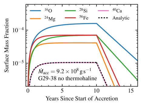
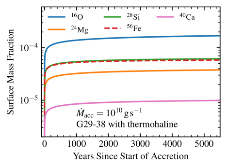
Figure 1: Left: MESA model of G29-38 matching observed abundances (Xu et al., 2014) after accreting earth-like composition at a total rate of ${\dot{M}_{\rm acc}=9.2\times 10^{8}\,\rm g\,s^{-1}}$ for 10 years to approach equilibrium surface abundances. Accretion ceases after 10 years to illustrate the exponential decay of observable pollution governed by diffusion in the absence of accretion. No thermohaline mixing is included in this model. Right: MESA model of G29-38 including thermohaline mixing accreting metals in the ratios observed at the WD surface at ${\dot{M}_{\rm acc}=10^{10}\,\rm g\,s^{-1}}$ for 5,000 years to approach observed surface abundances.

In Section 2, we discuss standard diffusion calculations and their relation to sedimentation in MESA models. In Section 3, we examine conditions for thermohaline instability in layers containing accreted metals and explore the impact of thermohaline mixing in our MESA models. In Section 4, we present the resulting implications for observed polluted WDs with hydrogen atmospheres. We find that WDs with $T_{\rm eff}\gtrsim 10,000\,\rm K$ require accretion rates several orders of magnitude larger than previously inferred, with the largest as high as ${\dot{M}_{\rm acc}\approx 10^{13}\,\rm g\,s^{-1}}$ when accounting for thermohaline mixing. In Section 5, we discuss avenues for extending and refining the grid of models.

2 Gravitational Sedimentation

In accretion-diffusion equilibrium, the observed metal abundances in the outer convective zone of a polluted WD are simply related to those in the accreted material. The timescale for convective mixing is rapid, so accreted material is quickly distributed throughout the convection zone. The observable mass fraction of an accreted pollutant $X_{{\rm cvz},i}$ is then related to the accretion rate $\dot{M}_{i}$ for that pollutant by (cf. Vauclair et al. 1979; Dupuis et al. 1993; Koester 2009)

$$M_{\rm cvz}\frac{dX_{{\rm cvz},i}}{dt}=\dot{M}_{i}-\frac{X_{{\rm cvz},i}M_{\rm cvz}}{\tau_{{\rm diff},i}}~{},$$ (1)

where the sedimentation time for element $i$ is

$$\tau_{{\rm diff},i}\equiv\frac{M_{\rm cvz}}{4\pi r^{2}\rho v_{{\rm diff},i}}~{},$$ (2)

and $v_{{\rm diff},i}$ is the downward sedimentation velocity of the accreted pollutant at the base of the surface convection zone, at density $\rho$ and radius $r$, where it sinks away from the fully mixed surface region.

Assuming $\tau_{{\rm diff},i}$, $\dot{M}_{i}$, and $M_{\rm cvz}$ are time independent, Equation (1) gives

$$X_{{\rm cvz},i}(t)=X_{{\rm cvz},i}(0)\,e^{-t/\tau_{{\rm diff},i}}+\frac{\dot{M}_{i}}{M_{\rm cvz}}\tau_{{\rm diff},i}\left(1-e^{-t/\tau_{{\rm diff},i}}\right)~{},$$ (3)

and for $t\gg\tau_{{\rm diff},i}$ the mass fraction approaches the equilibrium value

$$X_{{\rm eq},i}=\frac{\dot{M}_{i}}{M_{\rm cvz}}\tau_{{\rm diff},i}~{}.$$ (4)

Since sedimentation timescales in hydrogen WD atmospheres are short ($\tau_{\rm diff}\sim{\rm days}-10^{4}\,{\rm years}$, Koester 2009), Equation (4) is typically used to infer elemental accretion rates from observed abundances assuming $X_{{\rm obs},i}=X_{{\rm eq},i}$. A total accretion rate can be found simply by adding the individual contributions of each observed pollutant ($\dot{M}_{\rm acc}\equiv\sum_{i}\dot{M}_{i}$), or by scaling to a fiducial composition when other elements are not directly observed but are expected to be present (e.g. $\dot{M}_{\rm acc}=\dot{M}_{\rm Ca}/X_{\rm acc,Ca}$).

The theoretical ingredients for the preceding calculation are diffusion timescales and surface convection zone masses (Koester & Wilken, 2006; Koester, 2009). We calculate these as part of time-dependent WD evolutionary models with hydrogen atmospheres using MESA version 10398. In particular, our treatment of diffusion is based on a complete time-dependent solution of the Burgers equations for diffusion (Burgers, 1969), adapted to be appropriate for any degree of electron degeneracy in WDs as described in detail in Paxton et al. (2018). This treatment yields diffusion velocities for each species in the plasma everywhere in the stellar model. Our results for diffusion timescales and convection zone masses in WDs with hydrogen atmospheres are comparable to those of Koester (2009).

The convection prescription for our models is ML2 (Bohm & Cassinelli, 1971) with $\alpha_{\rm MLT}=0.8$. Our settings for surface boundary conditions rely on either a grey iterative procedure ($T_{\rm eff}>9,000\,\rm K$) described in Paxton et al. (2013), or the WD atmosphere tables in MESA ($T_{\rm eff}<9,000\,\rm K$), which are adapted from Rohrmann et al. (2012). Diffusion coefficients are those of Stanton & Murillo (2016) as implemented in Paxton et al. (2018), which produce comparable results to those of Paquette et al. (1986). More details are presented in a forthcoming paper. For WDs with no surface convection zone (${T_{\rm eff}\gtrsim 15,000\,\rm K}$), we take the surface region in which to evaluate $X_{\rm cvz}$ and $M_{\rm cvz}$ to be everywhere above the photosphere in the model (optical depth $\tau_{\rm Ross}=2/3$), with $\tau_{\rm diff}$ evaluated at the photosphere. See Gänsicke et al. (2012) for a thorough discussion justifying this choice.

The left panel of Figure 1 shows that a MESA model of an accretion episode with constant $\dot{M}_{\rm acc}=9.2\times 10^{8}\,\rm g\,s^{-1}$ (accreted mass fractions ${X_{\rm Fe}=0.307}$, ${X_{\rm O}=0.295}$, ${X_{\rm Mg}=0.199}$, $X_{\rm Si}=0.153$, $X_{\rm Ca}=0.046$) agrees with the prediction of Equation (3) when thermohaline mixing is not considered. This model is tuned to match the observed properties of G29-38 presented by Xu et al. (2014), including $T_{\rm eff}=11,820\,\rm K$, $\log g=8.4$, and the abundances presented in their Table 3. Our MESA model has diffusion timescales on the order of 1-2 years, roughly a factor of 5 longer than those reported by Xu et al. (2014) due to a larger surface convection zone in the MESA model ($M_{\rm cvz}=6\times 10^{-14}\,M_{\odot}$). This difference arises because convection zone depths are very sensitive to $T_{\rm eff}$ around the temperature for G29-38, and our models show growth of the surface convection zone slightly sooner as the WD cools compared to those of Koester (2009) in this regime. Hence, we infer an accretion rate that is $40\%$ larger than the value Xu et al. (2014) report, but we find excellent agreement with their relative diffusion timescales and composition of the accreted material.

3 Thermohaline Instability

Deal et al. (2013) and Wachlin et al. (2017) have noted that thermohaline mixing may significantly alter the accretion rates inferred from observed abundances in polluted WDs. Koester (2015) argued against the efficacy of this instability for a few cases. Here we show the regime in which it operates and its overall impact, which can be large.

3.1 Onset of the Instability Beneath the Convection Zone

Thermohaline instability can occur when fluid is stable to convection according to the Ledoux criterion, but has an inverted mean molecular weight gradient:

$$\nabla_{T}-\nabla_{\rm ad}<\frac{\varphi}{\delta}\nabla_{\mu}<0~{},$$ (5)

where $\nabla_{T}=(\partial\ln T/\partial\ln P)$ is the temperature gradient, ${\nabla_{\rm ad}=(\partial\ln T/\partial\ln P)_{s}}$ is the adiabatic temperature gradient, $\nabla_{\mu}=(\partial\ln\mu/\partial\ln P)$ is the mean molecular weight gradient, ${\varphi=(\partial\ln\rho/\partial\ln\mu)_{P,T}}$, and ${\delta=-(\partial\ln\rho/\partial\ln T)_{P,\mu}}$. A fluid satisfying Equation 5 alone is not guaranteed to experience thermohaline instability; the double-diffusive nature of the instability requires that microscopic particle transport between fluid elements be slow compared to thermal transport so that perturbed elements maintain their composition long enough for the instability to grow. This extra condition is (Baines & Gill, 1969; Brown et al., 2013; Garaud, 2018):

$$\frac{(\varphi/\delta)\nabla_{\mu}}{\nabla_{T}-\nabla_{\rm ad}}>\frac{\kappa_{\mu}}{\kappa_{T}}~{},$$ (6)

where $\kappa_{\mu}$ and $\kappa_{T}$ are the particle and thermal diffusivities.

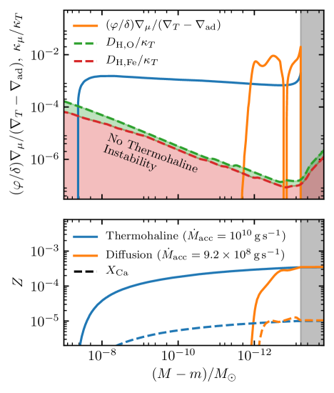
Figure 2: Profiles of quantities relevant to the onset of thermohaline instability in G29-38 models. The lower panel shows the metallicity profile with (blue) and without (orange) thermohaline mixing enabled according to Equation 9 with $\alpha_{\rm th}=1$, for the same models as shown in Figure 1. The upper panel shows the quantities necessary for evaluating the inequality given by Equation (6) in both cases, confirming that these profiles are thermohaline unstable. The gray shaded region represents the convective envelope.

The mean molecular weight gradient is inverted in the radiative zone beneath the outer convective layer of these polluted WDs. Heat is carried there via radiative diffusion, so

$$\kappa_{T}=\frac{4acT^{3}}{3\kappa\rho^{2}C_{P}}~{}.$$ (7)

We use the diffusion coefficients of oxygen or iron in hydrogen as representative of the particle diffusivity relevant for the mean molecular weight of a fluid element:

$$\kappa_{\mu}\approx D_{\rm H,O}\text{ or }D_{\rm H,Fe}~{}.$$ (8)

We obtain these coefficients from the same routines based on Stanton & Murillo (2016) that we use to calculate coefficients for element diffusion (Paxton et al., 2018).

Figure 2 shows the quantities relevant for evaluating the criterion for thermohaline instability given in Equation 6 for the G29-38 MESA model. The metallicity ($Z$) profile for the model is unstable according to Equation 6, and the result of enabling thermohaline mixing will be to mix a significant amount of the metals deeper into the star. A significantly larger accretion rate is then required to match the observed surface pollution in G29-38, similar to the results of Wachlin et al. (2017).

3.2 Outcomes when Thermohaline Mixing is Included

The default thermohaline mixing treatment in MESA (Paxton et al., 2013) follows Kippenhahn et al. (1980) in defining the mixing coefficient:

$$D_{\rm th}=\alpha_{\rm th}\kappa_{T}\frac{3}{2}\frac{(\varphi/\delta)\nabla_{\mu}}{\nabla_{T}-\nabla_{\rm ad}}~{},$$ (9)

where $\alpha_{\rm th}$ is a dimensionless efficiency parameter that should be near unity. MESA also offers options for using more recent treatments of thermohaline mixing due to Traxler et al. (2011) and Brown et al. (2013), which attempt to constrain free parameters by calibrating effective 1D prescriptions to 3D simulations.

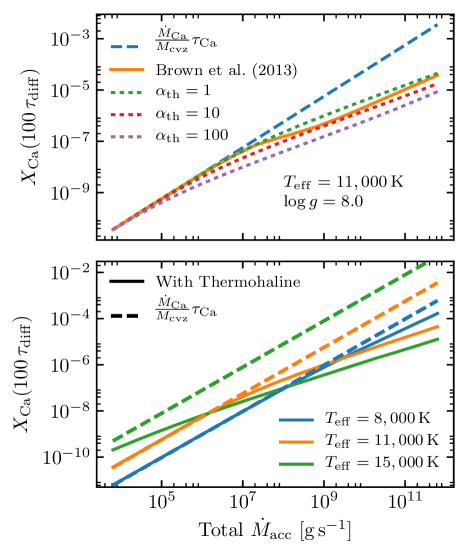
Figure 3: Surface Ca mass fraction after 100 diffusion timescales as a function of total metal accretion rate for a $0.6\,M_{\odot}$ ($\log g=8.0$) WD models accreting metals in bulk earth ratios. The upper panel shows several thermohaline prescriptions for a $T_{\rm eff}=11,000\,\rm K$ WD. The lower panel shows the WD at several temperatures for the thermohaline prescription of Equation 9 with $\alpha_{\rm th}=1$.

Figure 3 shows the surface Ca mass fraction in polluted $0.6\,M_{\odot}$ ($\log g=8.0$) WD models after accreting bulk earth material (McDonough, 2001) at $\dot{M}_{\rm acc}\in(10^{4},10^{12})\,\rm g\,s^{-1}$ for many diffusion timescales. These MESA models include element diffusion at all times. The upper panel includes models with thermohaline mixing according to Equation 9 (several values of $\alpha_{\rm th}$) and also according to Brown et al. (2013). These results suggest that Equation 9 reasonably captures the net effects of thermohaline mixing on pollution for efficiencies in the range ${1<\alpha_{\rm th}<10}$, though note that Vauclair & Théado (2012) have argued that more mixing should occur near the limit of instability to convection (${\nabla_{\mu}\sim\nabla_{T}-\nabla_{\rm ad}}$). We elect to employ the treatment of Equation 9 with $\alpha_{\rm th}=1$ for the models presented in the remainder of this work. Our choice of mixing prescription thus represents a reasonable but conservative estimate of the magnitude and total impact of thermohaline mixing for pollution.

The lower panel of Figure 3 shows the Ca pollution for models at several different values of $T_{\rm eff}$ using the thermohaline prescription of Equation 9 with $\alpha_{\rm th}=1$. Models with thin surface convection zones ($T_{\rm eff}=11,000\,\rm K;15,000\,\rm K$) experience significant dilution of surface metals due to thermohaline mixing, while models with larger surface convection zones ($T_{\rm eff}=8,000\,\rm K$) distribute accreted metals to an extent that $\nabla_{\mu}$ is rarely large enough to drive significant thermohaline mixing beneath the convection zone. In this case, diffusive sedimentation governs the timescale for settling and observed equilibrium abundances.

Unlike models with only element diffusion, those with thermohaline mixing do not approach a true equilibrium composition on a short timescale. Instead, they approach a quasi-steady state composition near the surface for timescales represented in Figure 3 ($\sim 100\,\tau_{\rm diff}$), but these quasi-steady abundances may vary by factors of a few if accretion continues over very long timescales ($\sim$Myr) as the thermohaline mixing region continues to extend deeper into the hydrogen envelope. Thermohaline mixing ceases to extend inward only when it encounters the diffusive tail of helium near the base of the hydrogen envelope. The $\nabla_{\mu}$ from this helium tail counteracts that from metals mixing inward, preventing any further thermohaline instability. For the hydrogen envelopes in our $M=0.6\,M_{\odot}$ WD models ($M_{\rm H}\approx 10^{-6}\,M_{\odot}$), the thermohaline mixing encounters the helium layer only after long periods ($\sim$Myr) of sustained high accretion rates ($\dot{M}_{\rm acc}\gtrsim 10^{10}\,\rm g\,s^{-1}$). Hence, this effect is not significant for the models we present in this work, but it may be important for WDs with much thinner hydrogen envelopes ($M_{\rm H}\lesssim 10^{-8}\,M_{\odot}$), where it could lead to higher observed surface pollution by preventing thermohaline mixing that would otherwise occur.

4 Accretion Rates and Compositions

In order to show the impact of our work on inferring accretion rates, we built an interpolating tool to map observed Ca abundances to total metal accretion rates for MESA runs that include thermohaline mixing and diffusion. The MESA runs used for this interpolation consist of 12 different WD models ($M=0.6\,M_{\odot}$, $\log g=8.0$) in the temperature range ${T_{\rm eff}\in(6000,20500)\,\rm K}$, each accreting bulk earth composition (McDonough, 2001) for 100 diffusion timescales at 17 rates in the range $\dot{M}_{\rm acc}\in(10^{4},10^{12})\,\rm g\,s^{-1}$, with diffusion enabled along with thermohaline mixing according to Equation 9 with $\alpha_{\rm th}=1$. At fixed $T_{\rm eff}$, a given observed Ca abundance corresponds to a unique value of total $\dot{M}_{\rm acc}$ (as seen in the lines in the lower panel of Figure 3), and we interpolate between results from MESA runs at different $T_{\rm eff}$ to yield a result for $\dot{M}_{\rm acc}$ as a function of $T_{\rm eff}$ and observed Ca abundance. Figure 4 shows the results of this procedure for inferring total $\dot{M}_{\rm acc}$ for the 38 polluted hydrogen atmosphere WDs given in Table 1 of Koester & Wilken (2006).

Figure 4 also compares against MESA calculations assuming only diffusion governs the equilibrium state, where we use Equation 4 to infer $\dot{M}_{\rm acc}$, and assume bulk earth abundances for the accreted material. For objects with ${T_{\rm eff}>10,000\,\rm K}$, the inferred accretion rate can increase by several orders of magnitude when accounting for thermohaline mixing, confirming the earlier work of Deal et al. (2013) and Wachlin et al. (2017).

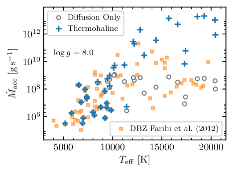
Figure 4: Accretion rates inferred with (blue crosses) and without (open circles) thermohaline mixing from the observed Ca abundances for the 38 WDs given in Table 1 of Koester & Wilken (2006), assuming $\log g=8.0$ and bulk earth composition in the accreting material. The orange points show the rates inferred for He atmosphere WDs by Farihi et al. (2012) for comparison.

Our models assume that the observed Ca is only a fraction of the total metals being accreted. This is important because all accreted metals participate in determining the $\nabla_{\mu}$ that drives thermohaline mixing. This should be justified, since Ca is often the most easily identifiable element in spectra even when other metals are present, and for the objects in which many metals are identified, compositions appear roughly consistent with bulk earth (Gänsicke et al., 2012; Jura & Young, 2014; Xu et al., 2014). Our inferences are also currently limited by the fact that all input models have a mass of $0.6\,M_{\odot}$ ($\log g=8.0$), which is not always consistent with the observed WDs. More MESA runs are necessary to build a tool that can interpolate over $\log g$ as well as $T_{\rm eff}$. However, we do not expect the small corrections due to different $\log g$’s to lead to qualitative changes in the several orders of magnitude effect seen in Figure 4.

For objects where multiple pollutants are observed, it should be possible to estimate relative accreted abundances, but there are two distinct regimes. For low accretion rates or thick convective envelopes where the thermohaline instability is not excited, the equilibrium state of each element is separately governed by Equation 4, so that the inferred relative abundance is related to observations by

$$\frac{X_{{\rm obs},1}}{X_{{\rm obs},2}}=\frac{\tau_{{\rm diff},1}X_{{\rm acc},1}}{\tau_{{\rm diff},2}X_{{\rm acc},2}}~{}.$$ (10)

However, when thermohaline mixing dominates over diffusion, the diffusion timescales play no role. Instead the mixing coefficient $D_{\rm th}$ applies equally to all elements, resulting in the observed relative abundances of metals matching the ratios in the accreted material.

Returning to MESA models of G29-38, when thermohaline mixing is included, we achieve a good match to observed pollution with an accretion rate of ${\dot{M}_{\rm acc}\gtrsim 10^{10}\,\rm g\,s^{-1}}$ (depending on thermohaline efficiency), higher than the value ${\dot{M}_{\rm acc}\approx 3\times 10^{9}\,\rm g\,s^{-1}}$ suggested by Wachlin et al. (2017). The significant thermohaline mixing also means that the best match to observed composition is achieved with a model that accretes metals in the same ratios as those observed at the photosphere, with no correction for relative diffusion timescales. Whereas the model without thermohaline mixing matches bulk earth composition remarkably well, models of G29-38 with thermohaline mixing imply a significantly more oxygen rich composition of the accreted material.

5 Conclusions and Future Work

Our MESA models indicate that inferred accretion rates in polluted WDs with hydrogen dominated atmospheres of $T_{\rm eff}\gtrsim 10,000\,\rm K$ require systematic increases due to thermohaline mixing, often by several orders of magnitude. These higher rates can be tested, especially via X-ray observations (Farihi et al., 2018). Very thin hydrogen envelopes ($M_{\rm H}\lesssim 10^{-8}\,M_{\odot}$) are not considered in the models presented here, but are often poorly constrained. Such thin envelopes could impose a systematic effect on inferences by lessening the impact of thermohaline mixing, with smaller inferred accretion rates as the result. We have also assumed bulk earth composition, so objects that are very rich in Ca relative to other metals could also be revised downward.

Models that include significant corrections due to thermohaline mixing also show very different surface abundance ratios than those that only include diffusive sedimentation. Diffusion leads to a correction to observed compositions due to different sedimentation timescales for each element, while models where thermohaline mixing dominates over diffusion show metal ratios that match the accreted material.

We do not expect the thermohaline instability to play as large of a role on WDs with helium atmospheres due to their much thicker convective envelopes that distribute accreted metals much deeper into the star. Preliminary MESA runs with helium atmosphere WD models indicate that thermohaline mixing is unimportant for those with $T_{\rm eff}\lesssim 15,000\,\rm K$ due to their thick (${M_{\rm cvz}\gtrsim 10^{-6}\,M_{\odot}}$) convective envelopes. Hotter He atmosphere WDs may require some accretion rate corrections due to thermohaline mixing, but we expect the effect to remain modest. As predicted by Deal et al. (2013), our results in Figure 4 appear to resolve the discrepancy between inferred accretion rates in helium and hydrogen atmospheres that is seen in the work of Farihi et al. (2012).

The high accretion rates implied by our calculations here may pose problems for models that deliver accreted metals to the WD surface via Poynting-Robertson drag (Rafikov, 2011a). Models of runaway accretion events due to other disk processes have been proposed to account for high inferred accretion rates in helium atmosphere WDs (Rafikov, 2011b; Metzger et al., 2012), but it is unclear if these can account for the highest rates suggested in Figure 4.

Further work is necessary to extend our MESA models to cover the entire range of $\log g$ relevant to all observed polluted WDs. Future work will present this along with more details from MESA models for surface convection zone masses and individual diffusion timescales for many elements, as well as models for WDs with helium atmospheres. Surface mixing regions in polluted WDs may also be modified by convective overshoot (Tremblay et al., 2015; Kupka et al., 2018), and MESA models have the potential for including this effect as well.

References

- Baines & Gill (1969) Baines, P. G., & Gill, A. E. 1969, Journal of Fluid Mechanics, 37, 289
- Bohm & Cassinelli (1971) Bohm, K. H., & Cassinelli, J. 1971, A&A, 12, 21
- Brown et al. (2013) Brown, J. M., Garaud, P., & Stellmach, S. 2013, ApJ, 768, 34
- Burgers (1969) Burgers, J. M. 1969, Flow Equations for Composite Gases (New York: Academic Press)
- Chayer (2014) Chayer, P. 2014, MNRAS, 437, L95
- Chayer et al. (1995a) Chayer, P., Fontaine, G., & Wesemael, F. 1995a, ApJS, 99, 189
- Chayer et al. (1995b) Chayer, P., Vennes, S., Pradhan, A. K., et al. 1995b, ApJ, 454, 429
- Deal et al. (2013) Deal, M., Deheuvels, S., Vauclair, G., Vauclair, S., & Wachlin, F. C. 2013, A&A, 557, L12
- Dufour et al. (2012) Dufour, P., Kilic, M., Fontaine, G., et al. 2012, ApJ, 749, 6
- Dupuis et al. (1992) Dupuis, J., Fontaine, G., Pelletier, C., & Wesemael, F. 1992, ApJS, 82, 505
- Dupuis et al. (1993) —. 1993, ApJS, 84, 73
- Farihi (2016) Farihi, J. 2016, New A Rev., 71, 9
- Farihi et al. (2012) Farihi, J., Gänsicke, B. T., Wyatt, M. C., et al. 2012, MNRAS, 424, 464
- Farihi et al. (2009) Farihi, J., Jura, M., & Zuckerman, B. 2009, ApJ, 694, 805
- Farihi et al. (2018) Farihi, J., Fossati, L., Wheatley, P. J., et al. 2018, MNRAS, 474, 947
- Gänsicke et al. (2012) Gänsicke, B. T., Koester, D., Farihi, J., et al. 2012, MNRAS, 424, 333
- Garaud (2018) Garaud, P. 2018, Annual Review of Fluid Mechanics, 50, 275
- Girven et al. (2012) Girven, J., Brinkworth, C. S., Farihi, J., et al. 2012, ApJ, 749, 154
- Hunter (2007) Hunter, J. D. 2007, Computing In Science & Engineering, 9, 90
- Jones et al. (2001–) Jones, E., Oliphant, T., Peterson, P., et al. 2001–, SciPy: Open source scientific tools for Python, http://www.scipy.org/
- Jura (2003) Jura, M. 2003, ApJ, 584, L91
- Jura & Young (2014) Jura, M., & Young, E. D. 2014, Annual Review of Earth and Planetary Sciences, 42, 45
- Kippenhahn et al. (1980) Kippenhahn, R., Ruschenplatt, G., & Thomas, H.-C. 1980, A&A, 91, 175
- Koester (2009) Koester, D. 2009, A&A, 498, 517
- Koester (2015) Koester, D. 2015, in Astronomical Society of the Pacific Conference Series, Vol. 493, 19th European Workshop on White Dwarfs, ed. P. Dufour, P. Bergeron, & G. Fontaine, 129
- Koester et al. (2014) Koester, D., Gänsicke, B. T., & Farihi, J. 2014, A&A, 566, A34
- Koester & Wilken (2006) Koester, D., & Wilken, D. 2006, A&A, 453, 1051
- Kupka et al. (2018) Kupka, F., Zaussinger, F., & Montgomery, M. H. 2018, MNRAS, 474, 4660
- McDonough (2001) McDonough, W. F. 2001, in EarthQuake Thermodynamics and Phase Transformations in the Earth’s Interior, ed. E. R. Teisseyre & E. Majewski (San Diego: Academic Press), 3
- Metzger et al. (2012) Metzger, B. D., Rafikov, R. R., & Bochkarev, K. V. 2012, MNRAS, 423, 505
- Paquette et al. (1986) Paquette, C., Pelletier, C., Fontaine, G., & Michaud, G. 1986, ApJS, 61, 177
- Paxton et al. (2011) Paxton, B., Bildsten, L., Dotter, A., et al. 2011, ApJS, 192, 3
- Paxton et al. (2013) Paxton, B., Cantiello, M., Arras, P., et al. 2013, ApJS, 208, 4
- Paxton et al. (2015) Paxton, B., Marchant, P., Schwab, J., et al. 2015, ApJS, 220, 15
- Paxton et al. (2018) Paxton, B., Schwab, J., Bauer, E. B., et al. 2018, ApJS, 234, 34
- Rafikov (2011a) Rafikov, R. R. 2011a, ApJ, 732, L3
- Rafikov (2011b) —. 2011b, MNRAS, 416, L55
- Rohrmann et al. (2012) Rohrmann, R. D., Althaus, L. G., García-Berro, E., Córsico, A. H., & Miller Bertolami, M. M. 2012, A&A, 546, A119
- Stanton & Murillo (2016) Stanton, L. G., & Murillo, M. S. 2016, Phys. Rev. E, 93, 043203
- Traxler et al. (2011) Traxler, A., Garaud, P., & Stellmach, S. 2011, ApJ, 728, L29
- Tremblay et al. (2015) Tremblay, P.-E., Ludwig, H.-G., Freytag, B., et al. 2015, ApJ, 799, 142
- van der Walt et al. (2011) van der Walt, S., Colbert, S. C., & Varoquaux, G. 2011, Computing in Science & Engineering, 13, 22
- Vanderburg et al. (2015) Vanderburg, A., Johnson, J. A., Rappaport, S., et al. 2015, Nature, 526, 546
- Vauclair et al. (1979) Vauclair, G., Vauclair, S., & Greenstein, J. L. 1979, A&A, 80, 79
- Vauclair & Théado (2012) Vauclair, S., & Théado, S. 2012, ApJ, 753, 49
- Wachlin et al. (2017) Wachlin, F. C., Vauclair, G., Vauclair, S., & Althaus, L. G. 2017, A&A, 601, A13
- Wolf et al. (2017) Wolf, B., Bauer, E. B., & Schwab, J. 2017, wmwolf/MesaScript: A DSL for Writing MESA Inlists
- Xu et al. (2014) Xu, S., Jura, M., Koester, D., Klein, B., & Zuckerman, B. 2014, ApJ, 783, 79
- Zuckerman et al. (2007) Zuckerman, B., Koester, D., Melis, C., Hansen, B. M., & Jura, M. 2007, ApJ, 671, 872
- Zuckerman et al. (2003) Zuckerman, B., Koester, D., Reid, I. N., & Hünsch, M. 2003, ApJ, 596, 477