The non-perturbative phase diagram of the BMN matrix model

Abstract

We study the maximally supersymmetric plane wave matrix model (the BMN model) at finite temperature, $T$, and locate the high temperature phase boundary in the $(\mu,T)$ plane, where $\mu$ is the mass parameter. We find the first transition, as the system is cooled from high temperatures, is from an approximately $SO(9)$ symmetric phase to one where three matrices expand to form fuzzy spheres. For $\mu>3.0$ there is a second distinct transition at a lower temperature. The two transitions approach one another at smaller $\mu$ and merge in the vicinity of $\mu=3.0$. The resulting single transition curve then approaches the gauge/gravity prediction as $\mu$ is further decreased. We find a rough estimate of the transition, for all $\mu$, is given by a Padé resummation of the large-$\mu$, 3-loop perturbative, predictions. We find evidence that the transition at small $\mu$ is to an M5-brane phase of the theory.

1 Introduction

The BMN or plane wave matrix model model Berenstein:2003gb is the matrix model description of M-theory in discrete lightcone quantisation (DLCQ) when the M2-brane is propagating on an eleven dimensional plane wave background. This background preserves the maximal, sixteen, supersymmetries and is a massive deformation of the BFSS model Banks:1996vh ; Townsend:1995kk ; Susskind:1997cw .

In contrast to the BFSS model, the BMN matrix model has a discrete energy spectrum. It is conjectured to capture the entire dynamics of M-theory on the plane wave background and provide a non-perturbative definition of M-theory itself. Alternatively, it describes a system of D0-branes of IIA supergravity. It has BPS ground states, where the D0-branes expand to fuzzy spheres Dasgupta:2002ru ; Dasgupta:2002hx . In Maldacena:2002rb it is argued that the model also provides a regularisation of NS5/M5-branes.

For large $\mu$ the model becomes a supersymmetric gauged Gaussian model. Perturbation theory around this limiting model was performed up to three loop order Spradlin:2004sx ; Hadizadeh:2004bf and a large $\mu$ series for the transition in the Polyakov loop was developed. The dual gravitational theory was studied by perturbing around the BFSS dual geometry to linear order in small $\mu$ in Costa:2014wya and the corresponding dual gravity prediction for the transition was obtained to this order.

The gravity dual has a remarkably rich structure. At zero temperature it is described by bubbling geometries. The dual bubbling geometries are in eleven-dimensional supergravity compactified in one translationally invariant direction on the two-dimensional subspace LLM , or equivalently, in type IIA supergravity LM . The supergravity solutions are labeled by configuration of D2/M2 and NS5/M5 charges, discretely located on a one-dimensional subspace of the geometries, and each of them corresponds to a vacuum of the BMN model. In the large $N$ limit there are infinitely many solutions, and interesting special solutions, such as those corresponding to a single stack of D2/M2-branes or NS5/M5-branes, exist. At finite temperature, the system has a Hawking-Page transition—a transition between thermal and black hole spacetimes. The solution examined in Costa:2014wya has $S^{8}\times S^{1}$ horizon topology, which corresponds to the trivial vacuum in the BMN model, where the $S^{1}$ is the M-theory circle. It is surprisingly difficult to obtain general gravity solutions dual to the BMN model at finite temperature; even the solution in Costa:2014wya required numerical computations to obtain the free energy.

There is some understanding of the dual geometry from the gauge-theory side. Since the corresponding supergravity solutions are supposed to be obtained at low energy, the geometry should be constructed by a low-energy moduli operator in the gauge theory. In Asano:2014vba ; Asano:2014eca , the BPS operator that is expected to pick up the low-energy moduli was computed by the supersymmetric localisation method, and in the appropriate large-$N$ and strong coupling limit, it was found that its eigenvalue distribution satisfies the same integral equations as those determining the supergravity solution. These equations govern a non-trivial part of the dual metric, which is not determined by the isometry. Although these results successfully reproduced part of the supergravity solution, the dynamics of the emergence of those geometries, such as how the geometries are favoured or superposed as the temperature changes, is beyond the scope of such methods; therefore numerical simulations for the thermal theory provide important information on which geometry emerges naturally.

This paper is dedicated to obtaining a non-perturbative estimate of the high temperature phase boundary as a function of the mass parameter, $\mu$.

We find that a Padé resummation of the large $\mu$ perturbative series Hadizadeh:2004bf , with the assumption that the transition temperature goes to zero linearly with $\mu$, gives a result very close to that of the gravity calculations Costa:2014wya when expanded to linear order in small $\mu$. We use this interpolating Padé resummed curve as a guide to the location of the transition. In practice, we find it is an excellent guide, giving a reasonable approximate location of the transition for all values of $\mu$.

We study the BMN model non-perturbatively using Rational Hybrid Monte Carlo techniques. We map the phase diagram in the $(\mu,T)$ plane and determine the phase boundary as the system cools from the high temperature phase. We find that for large $\mu$, a sharp transition in the Polyakov loop locates the transition. However, for $\mu\sim 7.0$ we find that there are two phase boundaries and a new phase appears characterised by the Myers cubic term in the action acquiring a significant non-zero vacuum expectation value and the approximate $SO(9)$ symmetry no longer holds. We observe that this transition, which we call a Myers transition, is from a phase where the system fluctuates around the trivial configuration to one with fluctuations around expanded fuzzy spheres. In the transition region we observe that the system also fluctuates between different intermediate fuzzy sphere configurations. The transition should be in the universality class of the emergent geometry transitions discussed in DelgadilloBlando:2007vx ; DelgadilloBlando:2008vi ; OConnor:2013gfj . As the system is further cooled, with fixed $\mu$ (e.g. see $\mu=6.0$ in Figure 2), the Polyakov loop undergoes a separate transition but at a significantly lower temperature.

For $\mu<3.0$ we find the two transitions merge, and the combined transition is visible in both the Myers observable and the Polyakov loop and has a significant jump in the energy, $E=\langle H\rangle/N^{2}$, where $H$ is the Hamiltonian (see $\mu=2.0$ in Figure 3). For $\mu<3.0$, the transition in the Polyakov loop is rather difficult to observe but one can check that the eigenvalue density of the holonomy undergoes a transition from a gapped to a gapless spectrum as the system is cooled through the Myers transition temperature.

For small $\mu$, in the transition to a stable fuzzy sphere phase the Polyakov loop tends to increase sharply (see Figure 4) to a higher value before decreasing slowly. In turn, for fuzzy sphere backgrounds, the transition in the holonomy to a gapless phase occurs at a considerably lower temperature than the Myers transition; the latter transition coincides with the region where the holonomy associated with the trivial background becomes gapless. These different temperatures would correspond to different Hawking-Page transitions for different solutions in the gravity dual. This result is consistent with the upper bound for the critical temperature discussed in Costa:2014wya .

At large $N$ the system can be trapped in a given vacuum phase and the transition between such vacua, being a quantum effect, is suppressed. This stability was used in Honda:2013nfa to study ${\cal N}=4$ super Yang-Mills from the BMN model. The parameter region they used is located at lower temperatures than the Myers transition we observe, and thus consistent with our findings.

A key ingredient in ensuring that the system was in the preferred thermodynamic state, and not trapped in a false vacuum, was to cool the system adiabatically so that $E(T)$ remained a monotonic function of temperature.

In the intermediate $\mu$ regime the transition in the Myers term occurs at a significantly higher temperature than that predicted by our Padé curve while the transition in the Polyakov loop tracks it more closely. For smaller $\mu<2$ the Myers transition again approaches the Padé curve and begins to qualitatively agree with the dual gravity prediction Costa:2014wya . The observed transition also is from small to large Myers term. We interpret this as meaning that on the gravity side a spherical black hole becomes unstable to asymmetric deformations. To our knowledge, the relevant gravity solution describing the black hole corresponding to a fuzzy sphere vacuum has not yet been constructed.

The principal results of this paper are:

• A determination of the high temperature phase boundary of the BMN matrix model (see Figure 5).

• A Padé approximant estimate for the phase transition in the trivial vacuum.

• A detailed non-perturbative study of the model for $N=8$.

• An extrapolation to large $N$ of the Myers transition for $\mu=2.0$.

• For $\mu=2.0$ we find the Myers observable takes a finite, $N$ independent, non-zero value in the range studied. This suggests the transition can be interpreted as one to an M5-brane phase of the theory.

The paper is organised as follows. Section 2 describes the model and the Padé resummation of the large $\mu$ transition curve. Section 3 summarises our lattice formulation of the model. Section 4 discusses the observables we measure. Section 5 gives our results and describes the phase diagram we find. We end with some concluding remarks and discussion.

2 The BMN Model

The Euclidean thermal action for the BMN matrix model is given by

$$S[X,\psi]=N\int_{0}^{\beta}d\tau\,\operatorname{Tr}\Bigg{[} \frac{1}{2}D_{\tau}X^{i}D_{\tau}X^{i}-\frac{1}{4}\left([X^{r},X^{s}]+\frac{i\mu}{3}\varepsilon^{rst}X_{t}\right)^{2}$$

$$-\frac{1}{2}[X^{r},X^{m}]^{2}-\frac{1}{4}[X^{m},X^{n}]^{2}+\frac{1}{2}\left(\frac{\mu}{6}\right)^{2}X_{m}^{2}$$

$$+\frac{1}{2}\psi^{T}\mathcal{C}\left(D_{\tau}-\frac{i\mu}{4}\gamma^{567}\right)\psi-\frac{1}{2}\psi^{T}\mathcal{C}\gamma^{i}[X^{i},\psi]\Bigg{]},$$ (1)

where $i,j=1,\cdots,9$, $r,s=5,6,7$ and $m,n=1,\cdots,4,8,9$. The covariant derivative is defined by $D_{\tau}\cdot=\partial_{\tau}\cdot-i[A,\cdot]$ and $\mathcal{C}$ is the charge conjugation matrix of $Spin(9)$. In (1) we have rescaled $X^{i}$, $\psi$, $\tau$ and $A$ to absorb the dependence on the ’t Hooft coupling defined as $\lambda=Ng^{2}$ and we use $\beta=\lambda^{1/3}/T$ and $\mu=\mu_{0}/\lambda^{1/3}$ with $\mu_{0}$ the mass parameter of the plane wave geometry.

In the large $\mu$ limit the model (1) reduces to a supersymmetric Gaussian model. This simple Gaussian model undergoes a confinement-deconfinement phase transition as the temperature is lowered and a straightforward calculation gives the critical temperature in this limit as $T_{c}=\frac{\mu}{12\ln 3}$. This transition has been studied perturbatively in $1/\mu$ Spradlin:2004sx ; Hadizadeh:2004bf , where in a three loop calculation it was found that

$$T_{c}=\frac{\mu}{12\ln 3}\left\{1+\frac{2^{6}\times 5}{3}\frac{1}{\mu^{3}}-\left(\frac{23\times 19927}{2^{2}\times 3}+\frac{1765769\ln 3}{2^{4}\times 3^{2}}\right)\frac{1}{\mu^{6}}+\cdots\right\}.$$ (2)

This result, while reliable for large $\mu$ becomes untrustworthy as $\mu$ decreases and passes through zero for $\mu\simeq 13.4$. However, if we perform a Padé resummation of (2), assuming that $T_{c}\rightarrow 0$ linearly with $\mu$ as $\mu\rightarrow 0$, then we can rewrite (2) as

$$T_{c}=\frac{\mu}{12\ln 3}\left\{1+\frac{\frac{320}{3\mu^{3}}}{1+\frac{3}{320\mu^{3}}(\frac{458321}{12}+\frac{1765769\ln 3}{144})+\cdots}\right\},$$ (3)

which to linear order in small $\mu$ leads to the prediction

$$T_{c}=\frac{\mu}{12\ln 3}\left(1+\frac{1638400}{5499852+1765769\ln 3}\right)\simeq 0.0925579\mu.$$

This value is surprisingly close to

$$T_{c}=0.105905(57)\mu,$$ (4)

which was obtained from a rather involved dual gravity computation Costa:2014wya .

We use the Padé resummed result (3) as a guide to where one might expect the transition in the full model as $\mu$ is decreased and study the system using the rational hybrid Monte Carlo algorithm and a novel lattice discretisation described in LatticePaper .

The action (1) is minimised by the fuzzy sphere configurations,

$$X^{r}=-\frac{\mu}{3}J^{r}\quad\hbox{and}\quad X^{m}=0,$$ (5)

where $J^{r}$ are generators of $SU(2)$ in an arbitrary representation of total dimension $N$. These are BPS states and are protected ground states of the quantum Hamiltonian.

3 Lattice Formulation

We use a second order lattice discretisation of the model. In this formulation the time interval is replaced by a periodic lattice with $\Lambda$ sites. The matrices are located on the lattice site, and the lattice spacing is $a=\frac{\beta}{\Lambda}$.

The bosonic Laplacian is discretised using the lattice version

$$\Delta_{Bose}=\Delta+r_{b}a^{2}\Delta^{2}\,,\quad\hbox{where}\quad\Delta=\frac{2-e^{aD_{\tau}}-e^{-aD_{\tau}}}{a^{2}}\,.$$ (6)

In the fermionic action the Dirac operator is discretised as

$$D_{Lat}=K_{a}{\bf 1}_{16}-i\frac{\mu}{4}\gamma^{567}+\Sigma^{123}K_{w}\,,\quad\hbox{where}\quad\Sigma^{123}=i\gamma^{123}\,.$$ (7)

In (7)

$$K_{w}=r_{1f}a\Delta+r_{2f}a^{3}\Delta^{2}$$ (8)

is a Wilson term that suppresses fermionic doublers and

$$K_{a}=(1-r)\frac{e^{aD_{\tau}}-e^{-aD_{\tau}}}{2a}+r\frac{e^{2aD_{\tau}}-e^{-2aD_{\tau}}}{4a}\;$$ (9)

is a slightly more general discretisation of the derivative (the standard first order lattice derivative is recovered setting $r=0$). Here, $K_{a}$ is an anti-symmetric lattice operator while $K_{w}$ is symmetric. The overall Dirac operator ${\cal C}D_{Lat}$ is an anti-symmetry matrix. The charge conjugation matrix ${\cal C}$ is symmetric as are ${\cal C}\gamma^{i}$, while ${\cal C}\gamma^{ij}$ and ${\cal C}\gamma^{ijk}$ are the only anti-symmetric elements of the Clifford algebra. An alternative to using $\Sigma^{123}$ would have been to use $\Sigma^{89}=i\gamma^{89}$ which was the choice used in Anagnostopoulos:2007fw ; Catterall:2008yz ; Hanada ; Berkowitz:2016jlq ; Catterall:2010gf and our earlier code Filev:2015hia . However, $\Sigma^{89}$, in contrast to $\Sigma^{123}$, does not anti-commute with the mass term. Different components of the spinor then have different dispersion relations and $\mu$-dependent lattice effects which grow with $\mu$. We also found that using the $\Sigma^{89}$ prescription and a first order discretisation (i.e. where $r,r_{b}$ and $r_{2f}$ are zero) had large lattice effects for moderate values of $\mu$. We discuss details of our code and other technical issues in LatticePaper . The dispersion relations for the two options are illustrated in Figure 1, where one can see two curves for the $\Sigma^{89}$ prescription. As the temperature is lowered, with fixed $\Lambda$, the lattice spacing becomes larger and the splitting becomes more extreme.

In practice, the parameter values for our simulations were $r=-\frac{1}{3}$, $r_{1f}=0$, $r_{b}=\frac{1}{12}$, $r_{2f}\approx 0.148$. We chose $r=-\frac{1}{3}$ as it eliminates the cubic term in the expansion of $K_{a}$ and we found that choosing $r_{1f}=0$ minimised a lattice artifact in the inverse to $D_{Lat}$. For comparison the parameters used in Hanada were $r=-1$, $r_{1f}=0$, $r_{2f}=\frac{1}{4}$, $r_{b}=\frac{3}{4}$ and $\Sigma^{123}$ should be replaced with $\Sigma^{89}$.

For $\mu=6.0$ and different parameter choices, we performed tests of our $\Sigma^{123}$ formulation against the $\Sigma^{12}$ option. Fixing parameters to those of our current study we found results of the $\Sigma^{123}$ choice with $\Lambda=24$ comparable to the $\Sigma^{12}$ option with $\Lambda=48$.

In this paper we concentrate on $\Lambda=24$ and $N=8$; however, preliminary simulations comparing $\Lambda=24$ and $\Lambda=48$ show that the lattice effects are small especially for $\mu>4.0$ in the range of temperatures we studied. More generally, we found no observable difference in the location of the transitions between the two lattice sizes.

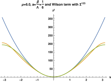
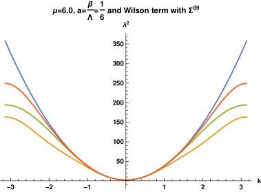
Figure 1: The two figures show the eigenvalues $k^{2}+\frac{\mu^{2}}{4}$ as the blue parabola, and $\Delta_{Bose}+\frac{\mu^{2}}{4}$ as the light green curve. The left figure then shows $D_{Lat}^{\dagger}D_{Lat}$ with $\Sigma^{123}$ Wilson term as the orange curve while the right figure shows the two distinct eigenvalues of $D_{Lat}^{\dagger}D_{Lat}$ with $\Sigma^{89}$ Wilson prescription as the red and orange curves. All plots are with $\mu=6.0$, $a=\frac{1}{6}$, $r=-\frac{1}{3}$, $r_{1f}=0$, $r_{b}=\frac{1}{12}$, $r_{2f}=0.1488$, the parameter values used in the simulations and a representative lattice spacing.

4 Observables

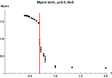
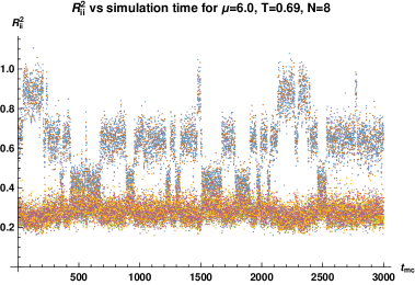
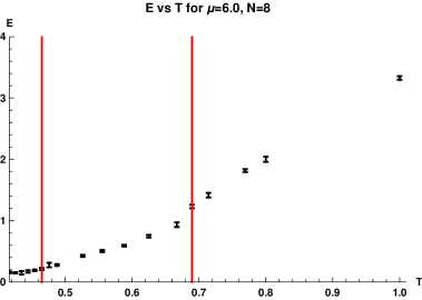
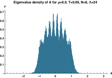
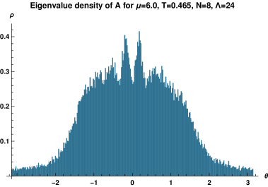
Figure 2: The figure shows the Myers observable, the Polyakov loop and the energy for $\mu=6.0$ and $N=8$. Two transitions occur at distinct temperatures, with the Myers transition occurring at $T_{c1}=0.690$, while the Polyakov transition, visible in both the Polyakov loop and eigenvalue density of the holonomy, occurs at $T_{c2}=0.465$. The top right figure shows $R^{2}_{ii}$ for each of the nine matrices at $T_{c1}=0.690$ marked as the red vertical line in the Myers plot and the higher temperature line in the energy plot. The upper points correspond to the $SO(3)$ matrices. The Polyakov loop shows a transition at $T_{c2}=0.465$, which is marked as the second lower temperature red line in the energy plot. The corresponding eigenvalue distributions for the holonomy at both transition temperatures are plotted, and one can see that Polyakov loop transition involves the eigenvalue distribution changing from gapped to ungapped.

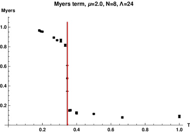
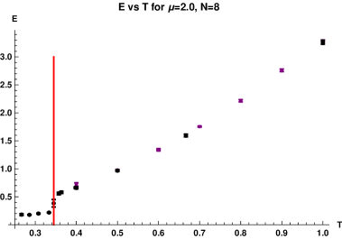
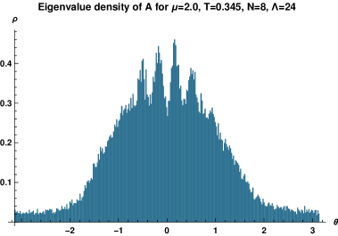
Figure 3: The figure shows the Myers observable, the energy as a function of temperature, the $R^{2}_{ii}$ for each $X_{i}$ as a function of Monte Carlo sweep and the spectrum of the holonomy $\rho$ for $\mu=2.0$, $N=8$, $\Lambda=24$. The red vertical line shows our measured value of the transition temperature $T_{c}=0.345$. One can see that the two transitions have merged to a single transition for this value of $\mu$. Since the mass is relatively small we have also included, in the energy plot, the energy of the BFSS system for $\mu=0$, $N=24$, $\Lambda=24$ (the purple points).

The BMN model is expected to have many phases and a rather complicated phase structure would be natural at low temperatures due to the multitude of zero energy BPS states. Our goal in this paper is to map the high temperature phase boundary to this region. We therefore study the system as the temperature is lowered, typically beginning our study at $T=2.0$ for a fixed $\mu$.

In the path integral formulation used in our study one can show, following the arguments of Asano:2016xsf , that the energy is given by

$$E=\left\langle\frac{1}{N\beta}\int_{0}^{\beta}d\tau\,\operatorname{Tr}\Bigg{[}-\frac{3}{4}[X^{i},X^{j}]^{2}\right. -\frac{5i\mu}{6}\varepsilon_{rst}X^{r}X^{s}X^{t}+\left(\frac{\mu}{6}\right)^{2}(X^{m})^{2}$$

$$\left.+\left(\frac{\mu}{3}\right)^{2}(X^{r})^{2}-\frac{3}{4}\psi^{T}\mathcal{C}\gamma^{i}[X^{i},\psi]-\frac{i\mu}{8}\psi^{T}\mathcal{C}\gamma^{567}\psi\Bigg{]}\right\rangle\,.$$ (10)

For the BFSS model this reduces to

$$E=\left\langle\frac{1}{N\beta}\int_{0}^{\beta}d\tau\,\operatorname{Tr}\Bigg{[}-\frac{3}{4}[X^{i},X^{j}]^{2}-\frac{3}{4}\psi^{T}\mathcal{C}\gamma^{i}[X^{i},\psi]\Bigg{]}\right\rangle,$$ (11)

and (11) together with the Ward identity, which reads

$$2\langle S_{bos}\rangle+N\int_{0}^{\beta}d\tau\,\operatorname{Tr}\Bigg{[}-\frac{1}{2}[X^{i},X^{j}]^{2}-\frac{1}{2}\psi^{T}\mathcal{C}\gamma^{i}[X^{i},\psi]\Bigg{]}=9(N^{2}-1)\Lambda\,,$$ (12)

was typically used to express the energy without fermionic terms as

$$E=\frac{3}{N^{2}\beta}\left(\frac{9}{2}\Lambda(N^{2}-1)-\langle S_{bos}\rangle\right).$$ (13)

While this expression provides coding convenience it is not necessary as one can measure these fermionic observables using pseudo fermions. Also, note that (13) involves the difference of large numbers and is limited by the precision of the rational approximation to the fermionic contributions. Using this expression to determine the energy in a precision calculation can become a problem especially when approaching the continuum limit, a limit involving sending $\Lambda$ to infinity.

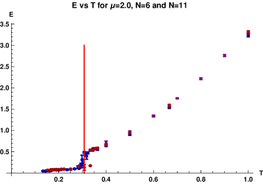
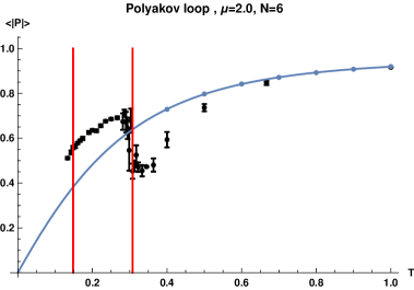
Figure 4: The left figure shows superimposed energy curves for $N=6$ and $N=11$. The right figure shows $\langle|P|\rangle$ for $N=6$, $\mu=2.0$ and $\Lambda=24$. The $N=6$ transition is taken to be at $T_{c}=0.31\pm 0.02$. Both plots include the BFSS energy (i.e. $\mu=0$) and $\langle|P|\rangle$ values for $N=24$, $\Lambda=24$. This data was used in the $1/N$ extrapolation in Figure 5.

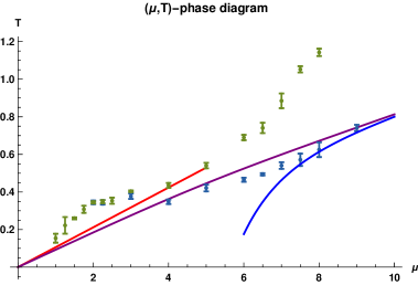
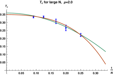
Figure 5: The left figure shows data for the two observed phase transitions. The green points are the observed values of the Myers transition and the dark blue points are the Polyakov transition, both were measured for $N=8$ and $\Lambda=24$. The blue curve is the large $\mu$ expansion of the critical temperature to 3 loops. The red line is the gauge gravity prediction and the purple curve is the Padé approximant obtained from the large mass expansion. The figure on the right shows our extrapolation of the critical temperature of the Myers transition from the observed values for $N=4,5,6,8$ and $N=11$ for $\mu=2.0$ and $\Lambda=24$. We use a quadratic extrapolation (green), given by $0.36-2.17x^{2}$ and quartic (red) given by $0.35-1.09x^{2}-15.26x^{4}$, which gives $T_{c}(\infty)=0.35\pm 0.01$.

In practice we find that the direct observable (11) behaves better numerically. For the BMN model we implement (10) directly using pseudo fermions following the strategy discussed in section 4.2 of Filev:2015hia and used in Asano:2016kxo . We also, for completeness, observe the BMN Ward identity analogue of (12).

The observables we follow are then: $E$ as defined in (10),

$${\rm Myers} =\left\langle\frac{i}{3N\beta}\int_{0}^{\beta}d\tau\epsilon_{rst}\operatorname{Tr}(X^{r}X^{s}X^{t})\right\rangle\,,$$ (14)

$$\left\langle|P|\right\rangle =\left\langle\frac{1}{N}|\operatorname{Tr}\left(\exp\left[i\beta A\right]\right)|\right\rangle\,,$$ (15)

$$\quad\qquad R^{2}_{ii} =\left\langle\frac{1}{N\beta}\int_{0}^{\beta}d\tau\operatorname{Tr}(X^{i}X^{i})\right\rangle\quad\hbox{(no sum on $i$).}$$ (16)

The energy and specific heat of the system, which due to supersymmetry, should both decrease to zero as $T$ approaches zero, are given by

$$N^{2}E=\langle H\rangle=-\partial_{\beta}\ln Z\quad\hbox{ and}\quad C=\langle(H-\langle H\rangle)^{2}\rangle=\partial^{2}_{\beta}\ln Z~{}\geq~{}0.$$ (17)

We see, furthermore, that $E$ must be a monotonic function of $T$. This proves especially useful in the simulations as tracking the energy as a function of $T$ was a crucial clue in identifying when the system transitioned to a new level. With this strategy and careful simulation as the transition was approached we identified the phase diagram as shown in Figure 5.

5 Results and Phase Diagram

For large $\mu$, e.g. $\mu=18.0$, we find that the transition is well tracked by the 3-loop perturbative result (2); however, deviations arise as $\mu$ is reduced. We concentrate our efforts on $\mu\leq 9.0$. We find that for $\mu\leq 6.5$ the system undergoes a phase transition from a small Myers observable to a large one and there is no longer an approximate $SO(9)$ symmetry. This is clear when observing $R^{2}_{ii}$, which at temperatures close to the transition has large fluctuations in the $SO(3)$ components (see Figure 2). A reasonable order parameter for this transition is the Myers observable (14), also shown in Figure 2 for $\mu=6.0$ as a function of temperature.

Figure 2 shows there are two separate transitions with the Myers transition occurring at the higher temperature. The figure also shows $R^{2}_{ii}$ for each of the nine matrices during a run corresponding to the transition value $T_{c1}=0.690$ marked as the red vertical line in the Myers plot and the higher temperature line in the energy plot. One can see that the $SO(3)$ matrices fluctuate between different fuzzy sphere vacua, while there are only small variations in the $SO(6)$ matrices, which are concentrated at smaller values.

The deconfinement transition is clear in the plot of the Polyakov loop and is measured to occur at $T_{c2}=0.465$. It is the second red line marked in the energy plot. The corresponding eigenvalue distributions of the holonomy for the two transition temperatures are plotted below and one can see that the confinement-deconfinement transition involves the eigenvalue distribution changing from gapped to ungapped. One can also see evidence for both transitions in the plot of $E$, though the Polyakov transition is less clear due to the relatively small jump in energy across this transition. However, as the temperature is lowered the transition in the energy becomes more pronounced and the two transitions approach, eventually effectively merging in the vicinity of $\mu=3.0$. Figure 3 shows our observables for $\mu=2.0$ with $N=8$ and $\Lambda=24$. Only one transition was observed and this transition is clear in the energy plot.

Once the system is cooled to a temperature below $T_{c1}$ the $SO(3)$ matrices settle into the thermodynamically favoured fuzzy sphere configuration, and the $SO(6)$ ones fluctuate around smaller values. Though larger fuzzy sphere vacua exist, further transitions between fuzzy sphere configurations were not observed as the system was cooled further.

We present our overall measured phase diagram in Figure 5. The figure is restricted to $N=8$ with $\Lambda=24$ and was determined from the Myers observable, Polyakov loop and energy observables. The simulations were performed beginning at $T=2.0$; then $T$ was slowly decreased for fixed $\mu$ using the thermalised input obtained at the higher temperature as an initial configuration for the lower $T$. The strategy of slowly decreasing the temperature for fixed $\mu$ proved crucial in determining the transition, as in many cases hysteresis made it difficult for the simulation to find the correct phase at the lower temperature. Which phase was correct was determined by carefully observing that the energy remained a monotonic function of $T$. The simulations indicate that the observed transitions are all first order, with a significant latent heat for $\mu=2.0$.

In the second graph in Figure 5 we focus on $\mu=2.0$ and extrapolate the critical temperature to large $N$ estimating that $T_{c}(\infty)=0.35\pm 0.01$, where the measured value for $N=8$ was $T_{c}(8)=0.345\pm 0.006$. From this example and preliminary results for other $\mu$ we expect that the large $N$ curve is shifted upwards slightly towards higher temperatures and we infer that the transition curve as measured in Figure 5 is a lower estimate for the large $N$ coexistence curve. Figure 4 shows the energy and Polyakov loop for $N=6$, with $\mu=2.0$. We see that the transition occurs at $T_{c}(6)=0.31\pm 0.02$, which is lower than $T_{c}(8)$; both are used in the $\frac{1}{N}$ extrapolation of Figure 5. Figure 4 also shows the Polyakov loop and we see it makes a sharp transition to a larger value. From this we infer that the fuzzy sphere configurations have typically larger Polyakov loop at a given temperature than the approximately $SO(9)$ symmetric phase. We further find that in this phase the holonomy becomes ungapped at $T\sim 0.15\pm 0.02$.

6 Conclusions

We have mapped an initial phase diagram for the BMN matrix model in the $(\mu,T)$ plane. We have concentrated on relatively small matrix sizes, with most of our data for $N=8$. The resulting diagram is presented in Figure 5.

We found that for small enough $N$ and large enough temperature ergodicity is not a problem. However, for large $N$ ergodicity is lost in the simulations, we therefore restricted our study to small $N$. For $N=6$ we tracked the system to relatively low temperatures (down to $T\sim 0.1$ with $\mu=2.0$). A little below the transition temperature it was apparent that maintaining ergodicity was beginning to be a problem as transitions between levels required rather lengthy simulations. For $N=8$ and $N=11$ there were difficulties with ergodicity, however, cooling the system in sufficiently small temperature intervals allowed us to access the transition. We suspect that going beyond $N=16$ would require new techniques to overcome these difficulties.

We have observed two transitions for larger values of $\mu$, which appear to merge for $\mu\sim 3.0$. The higher temperature transition curve, which shows the Myers transition curve, is the transition from the trivial vacuum to a non-trivial fuzzy sphere vacuum. In this transition the ground state consists of the $SO(3)$ matrices blowing up into fuzzy spheres and the transition has the characteristics of that discussed in DelgadilloBlando:2007vx ; DelgadilloBlando:2008vi ; OConnor:2013gfj . The Myers transition became very difficult to observe for $\mu>6.5$ as it occurred in a very narrow temperature interval. We have not successfully tracked it to very large $\mu$ and we suspect that, at least in the large $\mu$ region of the phase diagram, it is a finite matrix effect.

The second transition is observed in the Polyakov loop and is associated with the eigenvalue density of the gauge field, or holonomy, transitioning from gapped to ungapped (from covering a small interval of the unit circle to covering the entire circle). For $\mu\sim 6.0$ this occurs in a narrow temperature interval. However, as $\mu$ is lowered the Polyakov loop is not a monotonic function of temperature; it jumps upward at the Myers transition, where the system transitions to larger fuzzy sphere configurations. Each BPS ground state has its own typical value for the holonomy. In the Hamiltonian picture the holonomy implements the Gauss law constraint and is therefore sensitive to the density of accessible $SU(N)$ non-singlet states. It plays an essential rôle when there are many non-singlets around the relevant energy. One would expect that different fuzzy sphere configurations have different densities of non-singlets, which would account for the behaviour of the holonomy, as it is effectively probing these.

We found that as $\mu$ was decreased the two transitions merge at about $\mu\sim 3.0$. This single transition curve then approaches the Padé prediction (3) and the gauge/gravity Costa:2014wya prediction (4). We have not tracked the transition to $\mu$ less than $1.0$.

We find strong evidence that the Polyakov loop transition coincides with the Myers transition for $\mu<3.0$. Also, our results are in qualitative agreement with the gravity predictions of Costa:2014wya . However, we expect that better agreement over a larger range of $\mu$ would be obtained should a black hole solution dual to a general vacuum be available.

Another remarkable observation is that, at strong coupling, $\mu=2.0$, the Myers term seems to have a finite, non-zero value in the large-$N$ extrapolation. If one considers a typical vacuum as a representation with $m$ copies of the $k$ dimensional representation, it yields at low temperatures $\mathrm{Myers}\sim\frac{\mu^{3}}{3^{4}N}\operatorname{Tr}(J^{r}J^{r})\sim\mu^{3}(k^{2}-1)$. Such a configuration provides an example where this observable is non-zero and does not diverge, when $k$ is finite. Thus the easiest way to realise configurations that have finite Myers term at large $N$ is to have many copies of representations that fluctuate around a typical one of relatively small dimension. This should correspond to a state of five-branes Maldacena:2002rb , and in turn suggests that the Myers tranitions for $\mu<3$ can be regarded as a transition to a five-brane phase.

Our current study is clearly only the beginning. However, it indicates that an effort to construct such a black hole configuration in the dual gravitational theory, even a numerical one, would be very useful.

In the near future we plan to add D4-brane probes to the BMN model Kim:2002cr in analogy with our studies Asano:2016kxo ; Filev:2015cmz . This should give an alternative, more detailed probe, of the dual geometry.

References

- (1) D. E. Berenstein, J. M. Maldacena and H. S. Nastase, “Strings in flat space and pp waves from N=4 Super Yang Mills,” AIP Conf. Proc. 646 (2003) 3.
- (2) T. Banks, W. Fischler, S. H. Shenker and L. Susskind, “M theory as a matrix model: A Conjecture,” Phys. Rev. D 55, 5112 (1997) [hep-th/9610043].
- (3) P. K. Townsend, “The eleven-dimensional supermembrane revisited”, Phys. Lett. B350 (1995) 184 [hep-th/9501068].
- (4) L. Susskind, “Another conjecture about M(atrix) theory,” hep-th/9704080.
- (5) K. Dasgupta, M. M. Sheikh-Jabbari and M. Van Raamsdonk, “Matrix perturbation theory for M theory on a PP wave,” JHEP 0205 (2002) 056 doi:10.1088/1126-6708/2002/05/056 [hep-th/0205185].
- (6) K. Dasgupta, M. M. Sheikh-Jabbari and M. Van Raamsdonk, “Protected multiplets of M theory on a plane wave,” JHEP 0209 (2002) 021 doi:10.1088/1126-6708/2002/09/021 [hep-th/0207050].
- (7) J. M. Maldacena, M. M. Sheikh-Jabbari and M. Van Raamsdonk, “Transverse five-branes in matrix theory,” JHEP 0301 (2003) 038 doi:10.1088/1126-6708/2003/01/038 [hep-th/0211139].
- (8) M. Spradlin, M. Van Raamsdonk and A. Volovich, “Two-loop partition function in the planar plane-wave matrix model,” Phys. Lett. B 603, 239 (2004) doi:10.1016/j.physletb.2004.10.017 [hep-th/0409178].
- (9) S. Hadizadeh, B. Ramadanovic, G. W. Semenoff and D. Young, “Free energy and phase transition of the matrix model on a plane-wave,” Phys. Rev. D 71 (2005) 065016 doi:10.1103/PhysRevD.71.065016 [hep-th/0409318].
- (10) M. S. Costa, L. Greenspan, J. Penedones and J. Santos, “Thermodynamics of the BMN matrix model at strong coupling,” JHEP 1503 (2015) 069 doi:10.1007/JHEP03(2015)069 [arXiv:1411.5541 [hep-th]].
- (11) H. Lin, O. Lunin and J. M. Maldacena, “Bubbling AdS space and 1/2 BPS geometries,” JHEP 0410, 025 (2004) [hep-th/0409174].
- (12) H. Lin and J. M. Maldacena, “Fivebranes from gauge theory,” Phys. Rev. D 74, 084014 (2006) [hep-th/0509235].
- (13) Y. Asano, G. Ishiki, T. Okada and S. Shimasaki, “Emergent bubbling geometries in the plane wave matrix model,” JHEP 1405, 075 (2014) doi:10.1007/JHEP05(2014)075 [arXiv:1401.5079 [hep-th]].
- (14) Y. Asano, G. Ishiki and S. Shimasaki, “Emergent bubbling geometries in gauge theories with SU(2—4) symmetry,” JHEP 1409, 137 (2014) doi:10.1007/JHEP09(2014)137 [arXiv:1406.1337 [hep-th]].
- (15) Y. Asano, G. Ishiki, S. Shimasaki and S. Terashima, “On the transverse M5-branes in matrix theory,” Phys. Rev. D 96, 126003 (2017) [arXiv:1701.07140 [hep-th]].
- (16) Y. Asano, G. Ishiki, S. Shimasaki and S. Terashima, “Spherical transverse M5-branes from the plane wave matrix model,” JHEP 1802, 076 (2018) [arXiv:1711.07681 [hep-th]].
- (17) S. Catterall and G. van Anders, “First Results from Lattice Simulation of the PWMM,” JHEP 1009 (2010) 088 doi:10.1007/JHEP09(2010)088 [arXiv:1003.4952 [hep-th]].
- (18) N. Kawahara, J. Nishimura and K. Yoshida, “Dynamical aspects of the plane-wave matrix model at finite temperature,” JHEP 0606 (2006) 052 doi:10.1088/1126-6708/2006/06/052 [hep-th/0601170].
- (19) G. Ishiki, S. W. Kim, J. Nishimura and A. Tsuchiya, “Deconfinement phase transition in N=4 super Yang-Mills theory on R x S**3 from supersymmetric matrix quantum mechanics,” Phys. Rev. Lett. 102 (2009) 111601 doi:10.1103/PhysRevLett.102.111601 [arXiv:0810.2884 [hep-th]].
- (20) G. Ishiki, S. W. Kim, J. Nishimura and A. Tsuchiya, “Testing a novel large-N reduction for N=4 super Yang-Mills theory on R x S**3,” JHEP 0909 (2009) 029 doi:10.1088/1126-6708/2009/09/029 [arXiv:0907.1488 [hep-th]].
- (21) M. Honda, G. Ishiki, S. W. Kim, J. Nishimura and A. Tsuchiya, “Direct test of the AdS/CFT correspondence by Monte Carlo studies of N=4 super Yang-Mills theory,” JHEP 1311 (2013) 200 doi:10.1007/JHEP11(2013)200 [arXiv:1308.3525 [hep-th]].
- (22) R. Delgadillo-Blando, D. O’Connor and B. Ydri, “Geometry in Transition: A Model of Emergent Geometry,” Phys. Rev. Lett. 100, 201601 (2008) doi:10.1103/PhysRevLett.100.201601 [arXiv:0712.3011 [hep-th]].
- (23) R. Delgadillo-Blando, D. O’Connor and B. Ydri, “Matrix Models, Gauge Theory and Emergent Geometry,” JHEP 0905, 049 (2009) doi:10.1088/1126-6708/2009/05/049 [arXiv:0806.0558 [hep-th]].
- (24) D. O’Connor, B. P. Dolan and M. Vachovski, “Critical Behaviour of the Fuzzy Sphere,” JHEP 1312 (2013) 085 doi:10.1007/JHEP12(2013)085 [arXiv:1308.6512 [hep-th]].
- (25) Y. Asano and D. O’Connor, “Checking gauge/gravity duality with the BFSS model by different lattice discretisations”, in preparation.
- (26) K. N. Anagnostopoulos, M. Hanada, J. Nishimura and S. Takeuchi, “Monte Carlo studies of supersymmetric matrix quantum mechanics with sixteen supercharges at finite temperature,” Phys. Rev. Lett. 100, 021601 (2008) [arXiv:0707.4454 [hep-th]].
- (27) S. Catterall and T. Wiseman, “Black hole thermodynamics from simulations of lattice Yang-Mills theory,” Phys. Rev. D 78, 041502 (2008) [arXiv:0803.4273 [hep-th]].
- (28) M. Hanada, “A Users’ Manual of Monte Carlo Code for the Matrix Model of M-theory” https://sites.google.com/site/hanadamasanori/home/mmmm.
- (29) E. Berkowitz, E. Rinaldi, M. Hanada, G. Ishiki, S. Shimasaki and P. Vranas, Phys. Rev. D 94 (2016) no.9, 094501 doi:10.1103/PhysRevD.94.094501 [arXiv:1606.04951 [hep-lat]].
- (30) V. G. Filev and D. O’Connor, “The BFSS model on the lattice,” JHEP 1605 (2016) 167 doi:10.1007/JHEP05(2016)167 [arXiv:1506.01366 [hep-th]].
- (31) Y. Asano, V. G. Filev, S. Kováčik and D. O’Connor, “The Flavoured BFSS Model at High Temperature,” arXiv:1605.05597 [hep-th].
- (32) J. Maldacena and A. Milekhin, “To gauge or not to gauge?,” JHEP 1804 (2018) 084 doi:10.1007/JHEP04(2018)084 [arXiv:1802.00428 [hep-th]].
- (33) E. Berkowitz, M. Hanada, E. Rinaldi and P. Vranas, “Gauged And Ungauged: A Nonperturbative Test,” JHEP 1806, 124 (2018) doi:10.1007/JHEP06(2018)124 [arXiv:1802.02985 [hep-th]].
- (34) N. Kim, K. M. Lee and P. Yi, “Deformed matrix theories with N=8 and five-branes in the PP wave background,” JHEP 0211, 009 (2002) doi:10.1088/1126-6708/2002/11/009 [hep-th/0207264].
- (35) Y. Asano, V. G. Filev, S. Kováčik and D. O’Connor, “A computer test of holographic flavour dynamics. Part II,” JHEP 1803 (2018) 055 doi:10.1007/JHEP03(2018)055 [arXiv:1612.09281 [hep-th]].
- (36) V. G. Filev and D. O’Connor, “A Computer Test of Holographic Flavour Dynamics,” JHEP 1605, 122 (2016) doi:10.1007/JHEP05(2016)122 [arXiv:1512.02536 [hep-th]].