Automated computation of materials properties

Abstract

Materials informatics offers a promising pathway towards rational materials design, replacing the current trial-and-error approach and accelerating the development of new functional materials. Through the use of sophisticated data analysis techniques, underlying property trends can be identified, facilitating the formulation of new design rules. Such methods require large sets of consistently generated, programmatically accessible materials data. Computational materials design frameworks using standardized parameter sets are the ideal tools for producing such data. This work reviews the state-of-the-art in computational materials design, with a focus on these automated ab-initio frameworks. Features such as structural prototyping and automated error correction that enable rapid generation of large datasets are discussed, and the way in which integrated workflows can simplify the calculation of complex properties, such as thermal conductivity and mechanical stability, is demonstrated. The organization of large datasets composed of ab-initio calculations, and the tools that render them programmatically accessible for use in statistical learning applications, are also described. Finally, recent advances in leveraging existing data to predict novel functional materials, such as entropy stabilized ceramics, bulk metallic glasses, thermoelectrics, superalloys, and magnets, are surveyed.

1 Introduction

Materials informatics requires large repositories of materials data to identify trends in and correlations between materials properties, as well as for training machine learning models. Such patterns lead to the formulation of descriptors that guide rational materials design. Generating large databases of computational materials properties requires robust, integrated, automated frameworks [1]. Built-in error correction and standardized parameter sets enable the production and analysis of data without direct intervention from human researchers. Current examples of such frameworks include AFLOW (Automatic FLOW) [2, 3, 4, 5, 6, 7, 8, 9, 10], Materials Project [11, 12, 13, 14], OQMD (Open Quantum Materials Database) [15, 16, 17], the Computational Materials Repository [18] and its associated scripting interface ASE (Atomic Simulation Environment) [19], AiiDA (Automated Interactive Infrastructure and Database for Computational Science) [20, 21, 22], and the Open Materials Database at httk.openmaterialsdb.se with its associated High-Throughput Toolkit (HTTK). Other computational materials science resources include the aggregated repository maintained by the Novel Materials Discovery (NoMaD) Laboratory [23], the Materials Mine database available at www.materials-mine.com, and the Theoretical Crystallography Open Database (TCOD) [24]. For this data to be consumable by automated machine learning algorithms, it must be organized in programmatically accessible repositories [4, 5, 7, 11, 12, 15, 23]. These frameworks also contain modules that combine and analyze data from various calculations to predict complex thermomechanical phenomena, such as lattice thermal conductivity and mechanical stability.

Computational strategies have already had success in predicting materials for applications including photovoltaics [25], water-splitters [26], carbon capture and gas storage [27, 28], nuclear detection and scintillators [29, 30, 31, 32], topological insulators [33, 34], piezoelectrics [35, 36], thermoelectric materials [37, 38, 39, 40], catalysis [41], and battery cathode materials [42, 43, 44]. More recently, computational materials data has been combined with machine learning approaches to predict electronic and thermomechanical properties [45, 46], and to identify superconducting materials [47]. Descriptors are also being constructed to describe the formation of disordered materials, and have recently been used to predict the glass forming ability of binary alloy systems [48]. These successes demonstrate that accelerated materials design can be achieved by combining structured data sets generated using autonomous computational methods with intelligently formulated descriptors and machine learning.

2 Automated computational materials design frameworks

Rapid generation of materials data relies on automated frameworks such as AFLOW [2, 3, 4, 5, 6], Materials Project’s pymatgen [13] and atomate [14], OQMD [15, 16, 17], ASE [19], and AiiDA [21]. The general automated workflow is illustrated in Figure 1. These frameworks begin by creating the input files required by the electronic structure codes that perform the quantum-mechanics level calculations, where the initial geometry is generated by decorating structural prototypes (Figure 1(a, b)). They execute and monitor these calculations, reading any error messages written to the output files and diagnosing calculation failures. Depending on the nature of the errors, these frameworks are equipped with a catalog of prescribed solutions — enabling them to adjust the appropriate parameters and restart the calculations (Figure 1(c)). At the end of a successful calculation, the frameworks parse the output files to extract the relevant materials data such as total energy, electronic band gap, and relaxed cell volume. Finally, the calculated properties are organized and formatted for entry into machine-accessible, searchable and sortable databases.

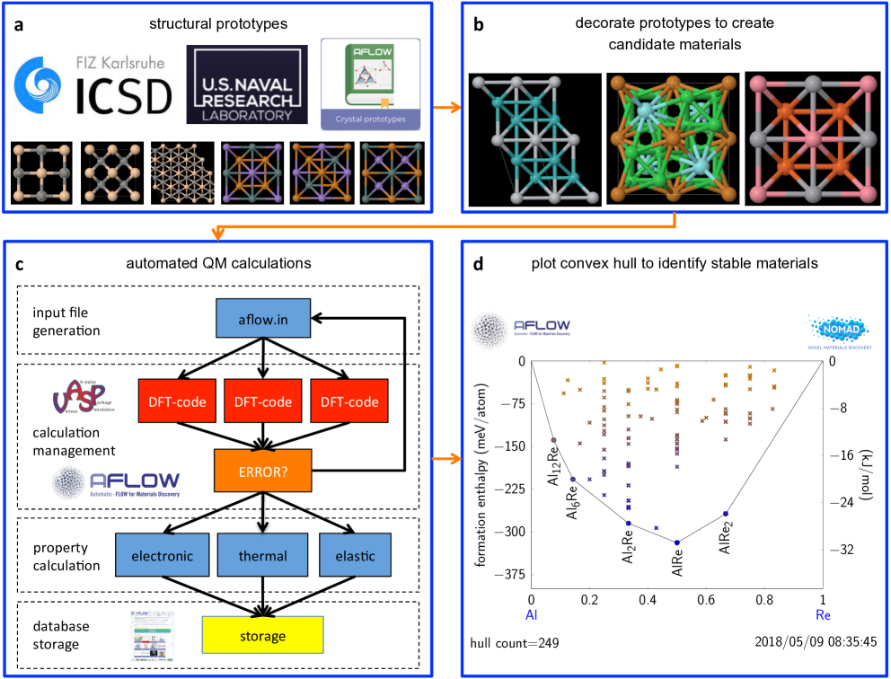
Figure 1: Computational materials data generation workflow. (a) Crystallographic prototypes are extracted from databases such as the ICSD or the NRL crystal structure library, or generated by enumeration algorithms. The illustrated examples are for the rocksalt, zincblende, wurtzite, Heusler, anti-Heusler and half-Heusler structures. (b) New candidate materials are generated by decorating the atomic sites with different elements. (c) Automated DFT calculations are used to optimize the geometric structure and calculate energetic, electronic, thermal, and elastic properties. Calculations are monitored to detect errors. The input parameters are adjusted to compensate for the problem and the calculation is re-run. Results are formatted and added to an online data repository to facilitate programmatic access. (d) Calculated data is used to plot the convex hull phase diagrams for each alloy system to identify stable compounds.

In addition to running and managing the quantum-mechanics level calculations, the frameworks also maintain a broad selection of post-processing libraries for extracting additional properties, such as calculating x-ray diffraction (XRD) spectra from relaxed atomic coordinates, and the formation enthalpies for the convex hull analysis to identify stable compounds (Figure 1(d)). Results from calculations of distorted structures can be combined to calculate thermal and elastic properties [2, 49, 50, 51], and results from different compositions and structural phases can be amalgamated to generate thermodynamic phase diagrams.

2.1 Generating and using databases for materials discovery

A major aim of high-throughput computational materials science is to identify new, thermodynamically stable compounds. This requires the generation of new materials structures, which have not been previously reported in the literature, to populate the databases. The accuracy of analyses involving sets of structures, such as that used to determine thermodynamic stability, is contingent on sufficient exploration of the full range of possibilities. Therefore, autonomous materials design frameworks such as AFLOW use crystallographic prototypes to generate new materials entries consistently and reproducibly.

Crystallographic prototypes are the basic building blocks used to generate the wide range of materials entries involved in computational materials discovery. These prototypes are based on i. structures commonly observed in nature [52, 53, 54], such as the rocksalt, zincblende, wurtzite or Heusler structures illustrated in Figure 1(b), as well as ii. hypothetical structures, such as those enumerated by the methods described in Refs. 55, 56. The AFLOW Library of Crystallographic Prototypes [54] is also available online at aflow.org/CrystalDatabase/, where users can choose from hundreds of crystal prototypes with adjustable parameters, and which can be decorated to generate new input structures for materials science calculations.

New materials are then generated by decorating the various atomic sites in the crystallographic prototype with different elements. These decorated prototypes serve as the structural input for ab-initio calculations. A full relaxation of the geometries and energy determination follows, from which phase diagrams for stability analyses can be constructed. The resulting materials data are then stored in an online data repository for future consideration.

The phase diagram of a given alloy system can be approximated by considering the low-temperature limit in which the behavior of the system is dictated by the ground state [57, 58]. In compositional space, the lower-half convex hull defines the minimum energy surface and the ground-state configurations of the system. All non-ground-state stoichiometries are unstable, with the decomposition described by the hull facet directly below it. In the case of a binary system, the facet is a tie-line as illustrated in Figure 2(a). The energy gained from this decomposition is geometrically represented by the (vertical-)distance of the compound from the facet and quantifies the excitation energy involved in forming this compound. While the minimum energy surface changes at finite temperature (favoring disordered structures), the $T=0$ K excitation energy serves as a reasonable descriptor for relative thermodynamic stability [59]. This analysis generates valuable information such as ground-state structures, excitation energies, and phase coexistence for storage in the online data repository. This stability data can be visualized and displayed by online modules, such as those developed by AFLOW [59], the Materials Project [60], and the OQMD [61, 16]. An example visualization from AFLOW is shown in Figure 2(b).

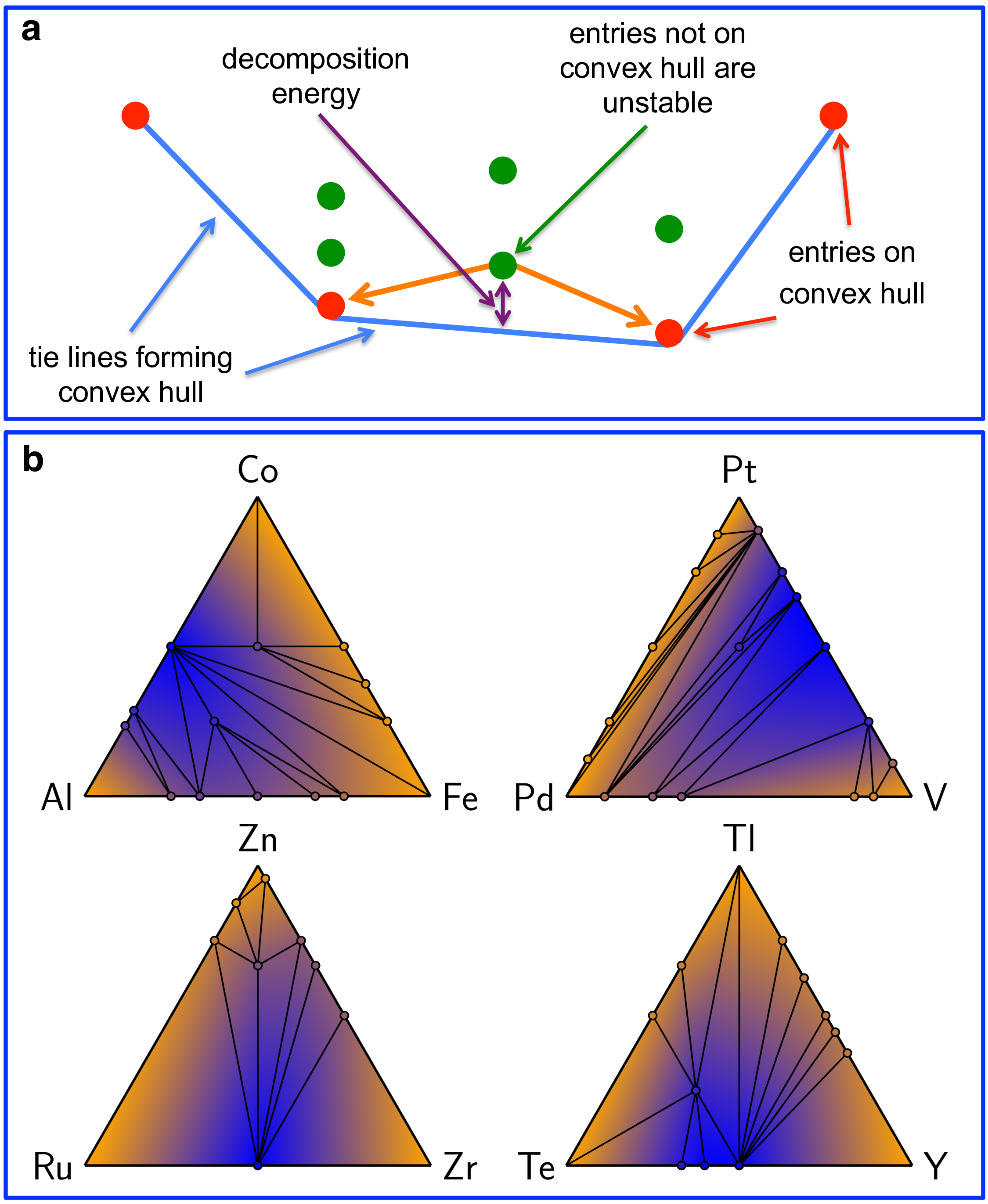
Figure 2: Convex hull phase diagrams for multicomponent alloys systems. (a) Schematic illustrating construction of convex hull for a general binary alloy system $A_{x}B_{1-x}$. Ground state structures are depicted as red points, with the minimum energy surface outlined with blue lines. The minimum energy surface is formed by connecting the lowest energy structures with tie lines which form a convex hull. Unstable structures are shown in green, with the decomposition reaction indicated by orange arrows, and the decomposition energy indicated in purple. (b) Example ternary convex hulls as generated by AFLOW.

Convex hull phase diagrams have been used to discover new thermodynamically stable compounds in a wide range of alloy systems, including hafnium [62, 63], rhodium [64], rhenium [65], ruthenium [66], and technetium [67] with various transition metals, as well as the Co-Pt system [68]. Magnesium alloy systems such as the lightweight Li-Mg system [69] and 34 other Mg-based systems [70] have also been investigated. This approach has also been used to calculate the solubility of elements in titanium alloys [71], to study the effect of hydrogen on phase separation in iron-vanadium [72], and to find new superhard tungsten nitride compounds [73]. The data has been employed to generate structure maps for hcp metals [74], as well as to search for new stable compounds with the Pt₈Ti phase [75], and with the $L1_{1}$ and $L1_{3}$ crystal structures [76]. Note that even if a structure does not lie on the ground state convex hull, this does not rule out its existence. It may be synthesizable under specific temperature and pressure conditions, and then be metastable under ambient conditions.

2.2 Standardized protocols for automated data generation

Standard calculation protocols and parameters sets [6] are essential to the identification of trends and correlations among materials properties. The workhorse method for calculating quantum-mechanically resolved materials properties is density functional theory (DFT). DFT is based on the Hohenberg-Kohn theorem [77], which proves that for a ground state system, the potential energy is a unique functional of the density: $V(\vec{r})=V(\rho(\vec{r}))$. This allows for the charge density $\rho(\vec{r})$ to be used as the central variable for the calculations rather than the many-body wave function $\Psi(\vec{r_{1}},\vec{r_{2}},...,\vec{r_{N}})$, dramatically reducing the number of degrees of freedom in the calculation.

The Kohn-Sham equations [78] map the $n$ coupled equations for the system of $n$ interacting particles onto a system of $n$ independent equations for $n$ non-interacting particles:

$$\left[-\frac{\hbar^{2}}{2m}\nabla^{2}+V_{s}(\vec{r})\right]\phi_{i}(\vec{r})=\varepsilon_{i}\phi_{i}(\vec{r}),$$ (1)

where $\phi_{i}(\vec{r})$ are the non-interacting Kohn-Sham eigenfunctions and $\varepsilon_{i}$ are their eigenenergies. $V_{s}(\vec{r})$ is the Kohn-Sham potential:

$$V_{s}(\vec{r})=V(\vec{r})+\int e^{2}\frac{\rho_{s}(\vec{r^{\prime}})}{|\vec{r}-\vec{r^{\prime}}|}d^{3}\vec{r^{\prime}}+V_{\begin{subarray}{c}\scalebox{0.6}{XC}\end{subarray}}\left[\rho_{s}(\vec{r})\right],$$ (2)

where $V(\vec{r})$ is the external potential (which includes influences of the nuclei, applied fields, and the core electrons when pseudopotentials are used), the second term is the direct Coulomb potential, and $V_{\begin{subarray}{c}\scalebox{0.6}{XC}\end{subarray}}\left[\rho_{s}(\vec{r})\right]$ is the exchange-correlation term.

The mapping onto a system of $n$ non-interacting particles comes at the cost of introducing the exchange-correlation potential $V_{\begin{subarray}{c}\scalebox{0.6}{XC}\end{subarray}}\left[\rho_{s}(\vec{r})\right]$, the exact form of which is unknown and must be approximated. The simplest approximation is the local density approximation (LDA) [79], in which the magnitude of the exchange-correlation energy at a particular point in space is assumed to be proportional to the magnitude of the density at that point in space. Despite its simplicity, LDA produces realistic results for atomic structure, elastic and vibrational properties for a wide range of systems. However, it tends to overestimate the binding energies of materials, even putting crystal bulk phases in the wrong energetic order [80]. Beyond LDA is the Generalized Gradient Approximation (GGA), in which the exchange correlation term is a functional of the charge density and its gradient at each point in space. There are several forms of GGA  including those developed by Perdew, Burke and Ernzerhof (PBE, [81]), or by Lee, Yang and Parr (LYP, [82]). A more recent development is the meta-GGA Strongly Constrained and Appropriately Normed (SCAN) functional [83], which satisfies all 17 known exact constraints on meta-GGA functionals.

The major limitations of LDA and GGA include their inability to adequately describe systems with strongly correlated or localized electrons, due to the local and semilocal nature of the functionals. Treatments include the Hubbard $U$ corrections [84, 85], self-interaction corrections [79] and hybrid functionals such as Becke’s 3-parameter modification of LYP (B3LYP, [86]), and that of Heyd, Scuseria and Ernzerhof (HSE, [87]).

Within the context of ab-initio structure prediction calculations, GGA-PBE is the usual standard since it tends to produce accurate geometries and lattice constants [57]. For accounting for strong correlation effects, the DFT$+U$ method [84, 85] is often favored in large-scale automated database generation due to its low computational overhead. However, the traditional DFT$+U$ procedure requires the addition of an empirical factor to the potential [84, 85]. Recently, methods have been implemented to calculate the $U$ parameter self-consistently from first-principles, such as the ACBN0 functional [88].

DFT also suffers from an inadequate description of excited/unoccupied states, as the theory is fundamentally based on the ground state. Extensions for describing excited states include time-dependent DFT (TDDFT) [89] and the GW correction [90]. However, these methods are typically much more expensive than standard DFT, and are not generally considered for large scale database generation.

At the technical implementation level, there are many DFT software packages available, including VASP [91, 92, 93, 94], QuantumESPRESSO [95, 96], ABINIT [97, 98], FHI–AIMS [99], SIESTA [100] and GAUSSIAN [101]. These codes are generally distinguished by the choice of basis set. There are two principle types of basis sets: plane waves, which take the form $\psi(\vec{r})=\sum e^{i\vec{k}\cdot\vec{r}}$, and local orbitals, formed by a sum over functions $\phi_{a}(\vec{r})$ localized at particular points in space, such as gaussians or numerical atomic orbitals [102]. Plane wave based packages include VASP, QuantumESPRESSO and ABINIT, and are generally better suited to periodic systems such as bulk inorganic materials. Local orbital based packages include FHI–AIMS, SIESTA and GAUSSIAN, and are generally better suited to non-periodic systems such as organic molecules. In the field of automated computational materials science, plane wave codes such as VASP are generally preferred: it is straightforward to automatically and systematically generate well-converged basis sets since there is only a single parameter to adjust, namely the cut-off energy determining the number of plane waves in the basis set. Local orbital basis sets tend to have far more independently adjustable degrees of freedom, such as the number of basis orbitals per atomic orbital as well as their respective cut-off radii, making the automated generation of reliable basis sets more difficult. Therefore, a typical standardized protocol for automated materials science calculations [6] relies on the VASP software package with a basis set cut-off energy higher than that recommended by the VASP potential files, in combination with the PBE formulation of GGA.

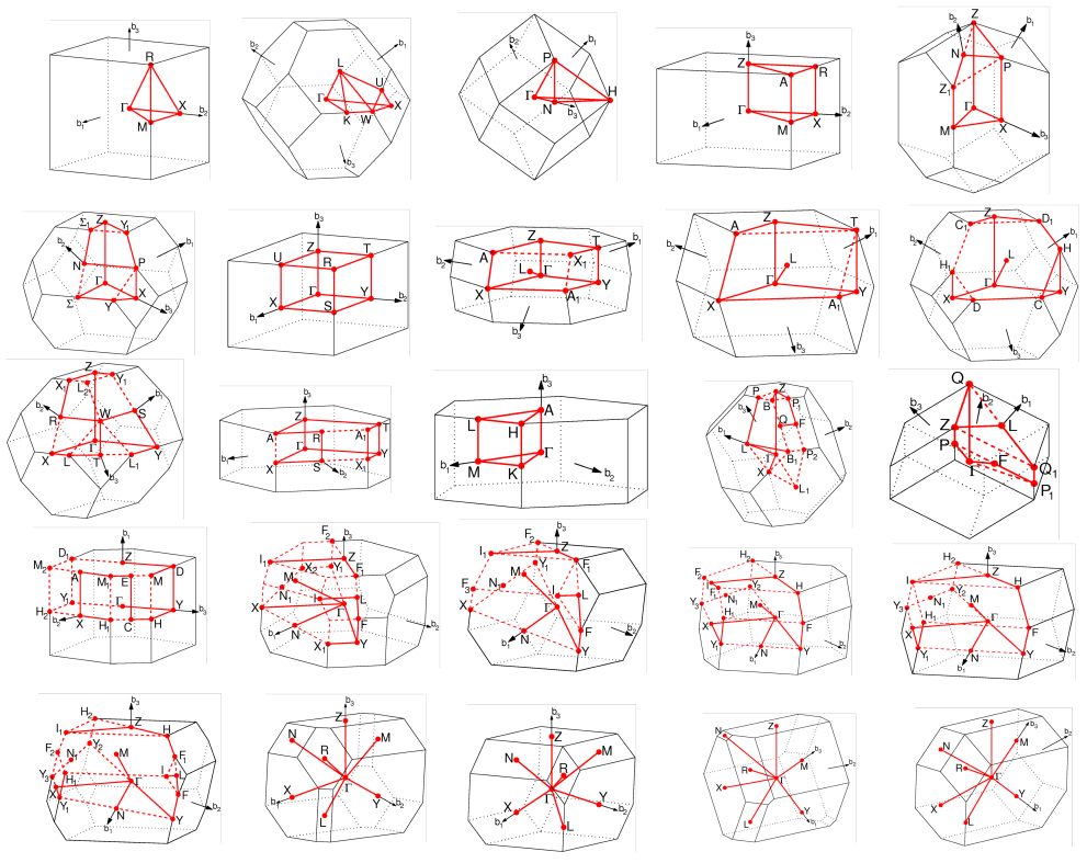
Figure 3: Standardized paths in reciprocal space for calculation of the electronic band structures for the 25 different lattice types [3].

Finally, it is necessary to automate the generation of the $k$-point grid and pathways in reciprocal space used for the calculation of forces, energies and the electronic band structure. In general, DFT codes use standardized methods such as the Monkhorst-Pack scheme [103] to generate reciprocal lattice $k$-point grids, although optimized grids have been calculated for different lattice types and are available online [104]. Optimizing $k$-point grid density is a computationally expensive process that is difficult to automate, so instead standardized grid densities based on the concept of “$k$-points per reciprocal atom” (KPPRA) are used. The KPPRA value is chosen to be sufficiently large to ensure convergence for all systems. Typical recommended values used for KPPRA range from 6,000 to 10,000 [6], so that a material with two atoms in the calculation cell will have a $k$-point mesh of at least 3,000 to 5,000 points. Standardized directions in reciprocal space have also been defined for the calculation of the band structure as illustrated in Figure 3 [3]. These paths are optimized to include all of the high-symmetry points of the lattice.

3 Integrated calculation of materials properties

Automated frameworks such as AFLOW combine the computational analysis of properties including symmetry, electronic structure, elasticity, and thermal behavior into integrated workflows. Crystal symmetry information is used to find the primitive cell to reduce the size of DFT calculations, to determine the appropriate paths in reciprocal space for electronic band structure calculations (see Figure 3, [3]), and to determine the set of inequivalent distortions for phonon and elasticity calculations. Thermal and elastic properties of materials are important for predicting the thermodynamic and mechanical stability of structural phases [105, 106, 107, 108] and assessing their importance for a variety of applications. Elastic properties such as the shear and bulk moduli are important for predicting the hardness of materials [109, 110], and thus their resistance to wear and distortion. Elasticity tensors can be used to predict the properties of composite materials [111, 112]. They are also important in geophysics for modeling the propagation of seismic waves in order to investigate the mineral composition of geological formations [106, 113, 114]. The lattice thermal conductivity $\left(\kappa_{\begin{subarray}{c}\scalebox{0.6}{L}\end{subarray}}\right)$ is a crucial design parameter in a wide range of important technologies, such as the development of new thermoelectric materials [115, 39, 116], heat sink materials for thermal management in electronic devices [117], and rewritable phase-change memories [118]. High thermal conductivity materials, which typically have a zincblende or diamond-like structure, are essential in microelectronic and nanoelectronic devices for achieving efficient heat removal [119], and have been intensively studied for the past few decades [120]. Low thermal conductivity materials constitute the basis of a new generation of thermoelectric materials and thermal barrier coatings [121].

The calculation of thermal and elastic properties offer an excellent example of the power of integrated computational materials design frameworks. With a single input file, these frameworks can automatically set-up and run calculations of different distorted cells, and combine the resulting energies and forces to calculate thermal and mechanical properties.

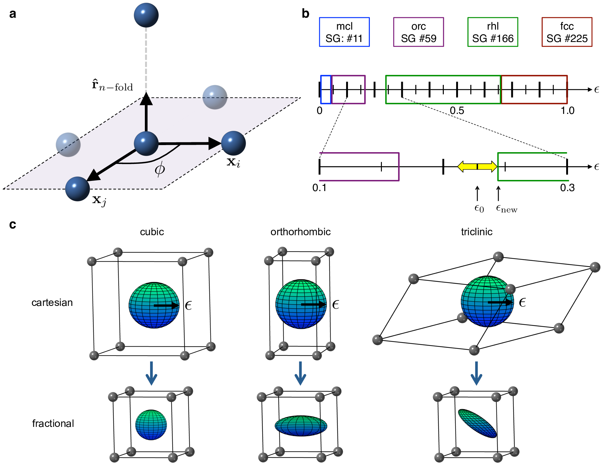
Figure 4: Challenges in autonomous symmetry analysis. (a) An illustration of a general $n$-fold symmetry operation. (b) Possible space group determinations with mapping tolerance $\epsilon$ for AgBr (ICSD #56551). (c) Warping of mapping tolerance sphere with a transformation from cartesian to fractional basis.

3.1 Autonomous symmetry analysis

Critical to any analysis of crystals is the accurate determination of the symmetry profile. For example, symmetry serves to i. validate the forms of the elastic constants and compliance tensors, where the crystal symmetry dictates equivalence or absence of specific tensor elements [122, 50, 107], and ii. reduce the number of ab-initio calculations needed for phonon calculations, where, in the case of the finite-displacement method, equivalent atoms and distortion directions are identified through factor group and site symmetry analyses [123].

Autonomous workflows for elasticity and vibrational characterizations therefore require a correspondingly robust symmetry analysis. Unfortunately, standard symmetry packages [124, 125, 126, 127], catering to different objectives, depend on tolerance-tuning to overcome numerical instabilities and atypical data — emanating from finite temperature measurements and uncertainty in experimentally reported observations. These tolerances are responsible for validating mappings and identifying isometries, such as the $n$-fold operator depicted in Figure 4(a). Some standard packages define separate tolerances for space, angle [127], and even operation type [124, 125, 126] (e.g., rotation versus inversion). Each parameter introduces a factorial expansion of unique inputs, which can result in distinct symmetry profiles as illustrated in Figure 4(b). By varying the spatial tolerance $\epsilon$, four different space groups can be observed for AgBr (ICSD #56551 ), if one is found at all. Gaps in the range, where no consistent symmetry profile can be resolved, are particularly problematic in automated frameworks, triggering critical failures in subsequent analyses.

Cell shape can also complicate mapping determinations. Anisotropies in the cell, such as skewness of lattice vectors, translate to distortions of fractional and reciprocal spaces. A uniform tolerance sphere in cartesian space, inside which points are considered mapped, generally warps to a sheared spheroid, as depicted in Figure 4(c). Hence, distances in these spaces are direction-dependent, compromising the integrity of rapid minimum-image determinations [129] and generally warranting prohibitively expensive algorithms [130]. Such failures can result in incommensurate symmetry profiles, where the real space lattice profile (e.g., bcc) does not match that of the reciprocal space (fcc).

The new AFLOW-SYM module [130] within AFLOW offers careful treatment of tolerances, with extensive validation schemes, to mitigate the aforementioned challenges. Although a user-defined tolerance input is still available, AFLOW defaults to one of two pre-defined tolerances, namely tight (standard) and loose. Should any discrepancies occur, these defaults are the starting values of a large tolerance scan, as shown in Figure 4(b). A number of validation schemes have been incorporated to catch such discrepancies. These checks are consistent with crystallographic group theory principles, validating operation types and cardinalities [131]. From considerations of different extreme cell shapes, a heuristic threshold has been defined to classify scenarios where mapping failures are likely to occur — based on skewness and mapping tolerance. When benchmarked against standard packages for over 54,000 structures in the Inorganic Crystal Structure Database, AFLOW-SYM consistently resolves the symmetry characterization most compatible with experimental observations [130].

Along with accuracy, AFLOW-SYM delivers a wealth of symmetry properties and representations to satisfy injection into any analysis or workflow. The full set of operators — including that of the point-, factor-, crystallographic point-, space groups, and site symmetries — are provided in matrix, axis-angle, matrix generator, and quaternion representations in both cartesian and fractional coordinates. A span of characterizations, organized by degree of symmetry-breaking, are available, including those of the lattice, superlattice, crystal, and crystal-spin. Space group and Wyckoff positions are also resolved. The full dataset is made available in both plain-text and JSON formats.

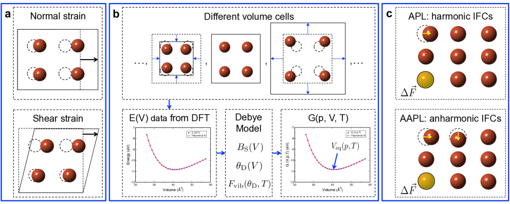
Figure 5: (a) AEL applies a set of independent normal and shear strains to the crystal structure to obtain the elastic constants. (b) AGL applies a set of isotropic strains to the unit cell to obtain energy versus volume data, which is fitted by a polynomial in order to calculate the bulk modulus as a function of volume, $B_{\mathrm{S}}(V)$. $B_{\mathrm{S}}(V)$ is then used to calculate the Debye temperature as a function of volume and thus the vibrational free energy as a function of temperature. The Gibbs free energy as a function of volume is then minimized for each pressure and temperature point to obtain the equilibrium volume and other thermomechanical properties. (c) APL obtains the harmonic interatomic force constants (IFCs) from supercell calculations where inequivalent atoms are displaced in inequivalent directions, and then the changes in the forces on the other atoms are calculated. The IFCs are then used to construct the dynamical matrix, which is diagonalized to obtain the phonon eigenmodes. AAPL calculates three-phonon scattering effects by performing supercell calculations where pairs of inequivalent atoms are displaced in inequivalent directions, and the changes in the forces on the other atoms in the supercell are calculated to obtain the third-order anharmonic IFCs.

3.2 Elastic Constants

There are two main methods for calculating the elastic constants based on the response of either the stress tensor or the total energy to a set of applied strains [50, 51, 132, 133, 133, 134]. Automated implementations of these methods are included in the AFLOW (referred to as the Automatic Elasticity Library, AEL [51]) and Materials Project frameworks [50].

To calculate the elastic tensor several different normal and shear strains should be applied to the calculation cell in each independent direction [50, 51], as illustrated in Figure 5(a). The resulting stress tensor elements $\sigma_{ij}$, obtained from the directional forces on the cell calculated with DFT, can then be fitted to the applied strains $\epsilon_{ij}$ to obtain the corresponding elastic constants $c_{ij}$ in the form of the stiffness tensor:

$$\left(\begin{array}[]{l}\sigma_{11}\\ \sigma_{22}\\ \sigma_{33}\\ \sigma_{23}\\ \sigma_{13}\\ \sigma_{12}\end{array}\right)=\left(\begin{array}[]{l l l l l l}c_{11}\ c_{12}\ c_{13}\ c_{14}\ c_{15}\ c_{16}\\ c_{12}\ c_{22}\ c_{23}\ c_{24}\ c_{25}\ c_{26}\\ c_{13}\ c_{23}\ c_{33}\ c_{34}\ c_{35}\ c_{36}\\ c_{14}\ c_{24}\ c_{34}\ c_{44}\ c_{45}\ c_{46}\\ c_{15}\ c_{25}\ c_{35}\ c_{45}\ c_{55}\ c_{56}\\ c_{16}\ c_{26}\ c_{36}\ c_{46}\ c_{56}\ c_{66}\end{array}\right)\left(\begin{array}[]{c}\epsilon_{11}\\ \epsilon_{22}\\ \epsilon_{33}\\ 2\epsilon_{23}\\ 2\epsilon_{13}\\ 2\epsilon_{12}\end{array}\right)$$ (3)

written in the $6\times 6$ Voigt notation using the mapping [106]: $11\mapsto 1$, $22\mapsto 2$, $33\mapsto 3$, $23\mapsto 4$, $13\mapsto 5$, $12\mapsto 6$. Symmetry analysis such as that provided by AFLOW-SYM can be used to reduce the number of required calculations by up to a factor of three in the case of cubic systems, as well as for verification of the computed tensors [107].

The elastic constants can then be used in the Voigt or Reuss approximations, which for polycrystalline materials correspond to assuming uniform strain and uniform stress respectively, and give the upper and lower bounds on the elastic moduli. In the Voigt approximation, the bulk modulus is given by

$$B_{{\begin{subarray}{c}\scalebox{0.6}{Voigt}\end{subarray}}}=\frac{1}{9}\left[(c_{11}+c_{22}+c_{33})+2(c_{12}+c_{23}+c_{13})\right],$$ (4)

and the shear modulus is given by

$$G_{{\begin{subarray}{c}\scalebox{0.6}{Voigt}\end{subarray}}}=\frac{1}{15}\left[(c_{11}+c_{22}+c_{33})-(c_{12}+c_{23}+c_{13})\right]+\\ \frac{1}{5}(c_{44}+c_{55}+c_{66}).$$ (5)

The Reuss approximation uses the elements of the compliance tensor $s_{ij}$ (the inverse of the stiffness tensor) to calculate the bulk modulus

$$\frac{1}{B_{{\begin{subarray}{c}\scalebox{0.6}{Reuss}\end{subarray}}}}=(s_{11}+s_{22}+s_{33})+2(s_{12}+s_{23}+s_{13}),$$ (6)

while the shear modulus is given by

$$\frac{15}{G_{{\begin{subarray}{c}\scalebox{0.6}{Reuss}\end{subarray}}}}=4(s_{11}+s_{22}+s_{33})-4(s_{12}+s_{23}+s_{13})+\\ +3(s_{44}+s_{55}+s_{66}).$$ (7)

The two approximations are combined to obtain the Voigt-Reuss-Hill (VRH) averages [135] for the bulk modulus

$$B_{{\begin{subarray}{c}\scalebox{0.6}{VRH}\end{subarray}}}=\frac{B_{{\begin{subarray}{c}\scalebox{0.6}{Voigt}\end{subarray}}}+B_{{\begin{subarray}{c}\scalebox{0.6}{Reuss}\end{subarray}}}}{2};$$ (8)

and the shear modulus

$$G_{{\begin{subarray}{c}\scalebox{0.6}{VRH}\end{subarray}}}=\frac{G_{{\begin{subarray}{c}\scalebox{0.6}{Voigt}\end{subarray}}}+G_{{\begin{subarray}{c}\scalebox{0.6}{Reuss}\end{subarray}}}}{2}.$$ (9)

The Poisson ratio $\nu$ is then given by

$$\nu=\frac{3B_{{\begin{subarray}{c}\scalebox{0.6}{VRH}\end{subarray}}}-2G_{{\begin{subarray}{c}\scalebox{0.6}{VRH}\end{subarray}}}}{6B_{{\begin{subarray}{c}\scalebox{0.6}{VRH}\end{subarray}}}+2G_{{\begin{subarray}{c}\scalebox{0.6}{VRH}\end{subarray}}}}.$$ (10)

3.3 Quasi-harmonic Debye-Grüneisen model

Thermal properties can be predicted by several different methods, such as the quasi-harmonic Debye-Grüneisen model which uses volume as a proxy for temperature [49], and by calculating the phonon dispersion from the dynamical matrix of IFCs [123].

The energy versus volume data from a set of simple static primitive cell calculations can be fitted to a quasi-harmonic Debye-Grüneisen model such as the “GIBBS” method [136, 49, 51] to obtain thermal properties, as demonstrated in Figure 5(b). This method has been implemented in the AFLOW framework in the form of the Automatic GIBBS Library (AGL).

First, the adiabatic bulk modulus $B_{\begin{subarray}{c}\scalebox{0.6}{S}\end{subarray}}$ as a function of cell volume $V$ is obtained either i. by fitting the $E_{\begin{subarray}{c}\scalebox{0.6}{DFT}\end{subarray}}(V)$ data to an equation of state (EOS), or ii. by taking the numerical second derivative of a polynomial fit of $E_{\begin{subarray}{c}\scalebox{0.6}{DFT}\end{subarray}}(V)$, which gives the static bulk modulus $B_{\mathrm{static}}$:

$$B_{\begin{subarray}{c}\scalebox{0.6}{S}\end{subarray}}(V) \approx B_{\mathrm{static}}(\vec{x})\approx B_{\mathrm{static}}(\vec{x}_{\begin{subarray}{c}\scalebox{0.6}{opt}\end{subarray}}(V))=$$

$$= V\left(\frac{\partial^{2}E(\vec{x}_{\begin{subarray}{c}\scalebox{0.6}{opt}\end{subarray}}(V))}{\partial V^{2}}\right)=V\left(\frac{\partial^{2}E(V)}{\partial V^{2}}\right).$$

Three different empirical EOS have been implemented within AGL: the Birch-Murnaghan EOS [137, 106, 136]; the Vinet EOS [138, 136]; and the Baonza-Cáceres-Núñez spinodal EOS [139, 136]. However, these EOS often introduce an additional source of error into the results since they are calibrated for specific sets of systems and pressure-temperature regimes. Recent studies have found the numerical calculation of $B$ to be just as, if not more, reliable as the empirical EOS [51]. Therefore, the numerical method is the default for the automated generation of thermomechanical properties for the AFLOW database.

The bulk modulus can then be used to calculate the Debye temperature as a function of volume:

$$\theta_{\begin{subarray}{c}\scalebox{0.6}{D}\end{subarray}}(V)=\frac{\hbar}{k_{\begin{subarray}{c}\scalebox{0.6}{B}\end{subarray}}}[6\pi^{2}V^{1/2}n]^{1/3}f(\nu)\sqrt{\frac{B_{\begin{subarray}{c}\scalebox{0.6}{S}\end{subarray}}}{M}},$$ (12)

where $M$ is the mass of the unit cell, and $f(\nu)$ is a function of the Poisson ratio $\nu$:

$$f(\nu)=\left\{3\left[2\left(\frac{2}{3}\!\cdot\!\frac{1+\nu}{1-2\nu}\right)^{3/2}+\left(\frac{1}{3}\!\cdot\!\frac{1+\nu}{1-\nu}\right)^{3/2}\right]^{-1}\right\}^{\frac{1}{3}}\!\!\!\!.$$ (13)

The integration offered by the AFLOW framework allows the value of $\nu$ required by this expression to be obtained directly and automatically from the AEL calculation (Equation 10).

To obtain the equilibrium volume at a particular $(p,T)$ point, the Gibbs free energy is minimized with respect to volume. In the quasi-harmonic approximation, the vibrational component of the free energy, $F_{\begin{subarray}{c}\scalebox{0.6}{vib}\end{subarray}}(\vec{x};T)$, is given by

$$F_{\begin{subarray}{c}\scalebox{0.6}{vib}\end{subarray}}(\vec{x};T)\!=\!\!\int_{0}^{\infty}\!\!\left[\frac{\hbar\omega}{2}\!+\!\frac{1}{\beta}\ \mathrm{log}\!\left(1\!-\!{\mathrm{e}}^{-\beta\hbar\omega}\right)\!\right]\!g(\vec{x};\omega)d\omega,$$ (14)

where $\beta=\left(k_{\begin{subarray}{c}\scalebox{0.6}{B}\end{subarray}}T\right)^{-1}$ and $g(\vec{x};\omega)$ is the phonon density of states, which depends on the system geometry $\vec{x}$. In the Debye-Grüneisen model, $F_{\begin{subarray}{c}\scalebox{0.6}{vib}\end{subarray}}$ can be written as

$$F_{\begin{subarray}{c}\scalebox{0.6}{vib}\end{subarray}}(\theta_{\begin{subarray}{c}\scalebox{0.6}{D}\end{subarray}};T)\!=\!\frac{n}{\beta}\!\left[\frac{9}{8}\frac{\theta_{\begin{subarray}{c}\scalebox{0.6}{D}\end{subarray}}}{T}\!+\!3\ \mathrm{log}\!\left(1\!-\!{\mathrm{e}}^{-\theta_{\begin{subarray}{c}\scalebox{0.6}{D}\end{subarray}}/T}\!\right)\!\!-\!\!D\left(\frac{\theta_{\begin{subarray}{c}\scalebox{0.6}{D}\end{subarray}}}{T}\right)\!\!\right],$$ (15)

where $D(\theta_{\begin{subarray}{c}\scalebox{0.6}{D}\end{subarray}}/T)$ is the Debye integral

$$D\left(\theta_{\begin{subarray}{c}\scalebox{0.6}{D}\end{subarray}}/T\right)=3\left(\frac{T}{\theta_{\begin{subarray}{c}\scalebox{0.6}{D}\end{subarray}}}\right)^{3}\int_{0}^{\theta_{\begin{subarray}{c}\scalebox{0.6}{D}\end{subarray}}/T}\frac{x^{3}}{e^{x}-1}dx.$$ (16)

Next, the full Gibbs free energy as a function of temperature and pressure is calculated

$${\sf G}(V;p,T)=E_{\begin{subarray}{c}\scalebox{0.6}{DFT}\end{subarray}}(V)+F_{\mathrm{vib}}(\theta_{\begin{subarray}{c}\scalebox{0.6}{D}\end{subarray}}(V);T)+pV,$$ (17)

and fitted by a polynomial in $V$, the minimum of which gives the equilibrium volume, $V_{\mathrm{eq}}$. Note that the symbol $G$ is used for shear modulus while G is used for the Gibbs free energy.

$\theta_{\begin{subarray}{c}\scalebox{0.6}{D}\end{subarray}}$ is then determined from its value at $V_{\mathrm{eq}}$, while other thermal properties such as the Grüneisen parameter can be calculated using the expression

$$\gamma=-\frac{V}{\theta_{\begin{subarray}{c}\scalebox{0.6}{D}\end{subarray}}}\frac{\partial\theta_{\begin{subarray}{c}\scalebox{0.6}{D}\end{subarray}}(V)}{\partial V}.$$ (18)

The specific heat capacity at constant volume can be obtained using the expression

$$C_{{\begin{subarray}{c}\scalebox{0.6}{V}\end{subarray}},{\begin{subarray}{c}\scalebox{0.6}{vib}\end{subarray}}}=3nk_{\begin{subarray}{c}\scalebox{0.6}{B}\end{subarray}}\left[4D\left(\frac{\theta_{\begin{subarray}{c}\scalebox{0.6}{D}\end{subarray}}}{T}\right)-\frac{3\theta_{\begin{subarray}{c}\scalebox{0.6}{D}\end{subarray}}/T}{e^{\theta_{\begin{subarray}{c}\scalebox{0.6}{D}\end{subarray}}/T}-1}\right],$$ (19)

while the specific heat capacity at constant pressure is given by

$$C_{{\rm p},{\begin{subarray}{c}\scalebox{0.6}{vib}\end{subarray}}}=C_{{\begin{subarray}{c}\scalebox{0.6}{V}\end{subarray}},{\begin{subarray}{c}\scalebox{0.6}{vib}\end{subarray}}}(1+\alpha\gamma T),$$ (20)

where $\alpha$ is the coefficient of thermal expansion

$$\alpha=\frac{\gamma C_{{\begin{subarray}{c}\scalebox{0.6}{V}\end{subarray}},{\begin{subarray}{c}\scalebox{0.6}{vib}\end{subarray}}}}{B_{\begin{subarray}{c}\scalebox{0.6}{T}\end{subarray}}V}.$$ (21)

The lattice thermal conductivity can be calculated using the Leibfried-Schlömann equation [140, 141, 142] using the Debye temperature and the Grüneisen parameter

$$\kappa_{\begin{subarray}{c}\scalebox{0.6}{L}\end{subarray}}(\theta_{\mathrm{a}}) = \frac{0.849\times 3\sqrt[3]{4}}{20\pi^{3}(1-0.514\gamma_{\mathrm{a}}^{-1}+0.228\gamma_{\mathrm{a}}^{-2})}$$

$$\times\left(\frac{k_{\begin{subarray}{c}\scalebox{0.6}{B}\end{subarray}}\theta_{\mathrm{a}}}{\hbar}\right)^{2}\frac{k_{\begin{subarray}{c}\scalebox{0.6}{B}\end{subarray}}mV^{\frac{1}{3}}}{\hbar\gamma_{\mathrm{a}}^{2}}.$$

where $V$ is the volume of the unit cell, $m$ is the average atomic mass, while $\theta_{\mathrm{a}}$ and $\gamma_{\mathrm{a}}$ are the acoustic Debye temperature and Grüneisen parameter obtained by only considering the acoustic modes, based on the assumption that the optical phonon modes in crystals do not contribute to heat transport [141, 142]. $\theta_{\mathrm{a}}$ and $\gamma_{\mathrm{a}}$ can be derived directly from the phonon DOS by only considering the acoustic modes [141, 143]. $\theta_{\mathrm{a}}$ can also be estimated from the traditional Debye temperature $\theta_{\begin{subarray}{c}\scalebox{0.6}{D}\end{subarray}}$ using the expression $\theta_{\mathrm{a}}=\theta_{\begin{subarray}{c}\scalebox{0.6}{D}\end{subarray}}n^{-\frac{1}{3}}$ [141, 142]. There is no simple way to extract $\gamma_{\mathrm{a}}$ from the traditional Grüneisen parameter, so the approximation $\gamma_{\mathrm{a}}=\gamma$ is used in the AEL-AGL approach to calculating the thermal conductivity.

The thermal conductivity at temperatures other than $\theta_{\mathrm{a}}$ is estimated using the expression [141, 142, 144]: $\kappa_{\begin{subarray}{c}\scalebox{0.6}{L}\end{subarray}}(T)=\kappa_{\begin{subarray}{c}\scalebox{0.6}{L}\end{subarray}}(\theta_{\mathrm{a}})\theta_{\mathrm{a}}/T$.

3.4 Harmonic Phonons

Thermal properties can also be obtained by directly calculating the phonon dispersion from the dynamical matrix of IFCs. The approach is implemented within the AFLOW Phonon Library (APL) [2]. The IFCs are determined from a set of supercell calculations in which the atoms are displaced from their equilibrium positions [123] as shown in Figure 5(c).

The IFCs derive from a Taylor expansion of the potential energy, $V$, of the crystal about the atoms’ equilibrium positions:

$$V=\left.V\right|_{\vec{r}(i,t)=0,\forall i}+\sum_{i,\alpha}\left.\frac{\partial V}{\partial r(i,t)^{\alpha}}\right|_{\vec{r}(i,t)=0,\forall i}r(i,t)^{\alpha}\\ +\frac{1}{2}\sum_{\begin{subarray}{c}i,\alpha,\\ j,\beta\end{subarray}}\left.\frac{\partial^{2}V}{\partial r(i,t)^{\alpha}\partial r(j,t)^{\beta}}\right|_{\vec{r}(i,t)=0,\forall i}r(i,t)^{\alpha}r(j,t)^{\beta}\\ +\ldots,$$ (23)

where $r(i,t)^{\alpha}$ is the $\alpha$-cartesian component ($\alpha=x,y,z$) of the time-dependent atomic displacement $\vec{r}(t)$ of the $i^{\mathrm{th}}$ atom about its equilibrium position, $\left.V\right|_{\vec{r}(i,t)=0,\forall i}$ is the potential energy of the crystal in its equilibrium configuration, $\left.\partial V/\partial r(i,t)^{\alpha}\right|_{\vec{r}(i,t)=0,\forall i}$ is the negative of the force acting in the $\alpha$ direction on atom $i$ in the equilibrium configuration (zero by definition), and $\left.\partial^{2}V/\partial r(i,t)^{\alpha}\partial r(j,t)^{\beta}\right|_{\vec{r}(i,t)=0,\forall i}$ constitute the IFCs $\phi(i,j)_{\alpha,\beta}$. To first approximation, $\phi(i,j)_{\alpha,\beta}$ is the negative of the force exerted in the $\alpha$ direction on atom $i$ when atom $j$ is displaced in the $\beta$ direction with all other atoms maintaining their equilibrium positions, as shown in Figure 5(c). All higher order terms are neglected in the harmonic approximation.

Correspondingly, the equations of motion of the lattice are as follows:

$$M(i)\ddot{r}(i,t)^{\alpha}=-\sum_{j,\beta}\phi(i,j)_{\alpha,\beta}r(j,t)^{\beta}\quad\forall i,\alpha,$$ (24)

and can be solved by a plane wave solution of the form

$$r(i,t)^{\alpha}=\frac{v(i)^{\alpha}}{\sqrt{M(i)}}e^{\mathrm{i}\left(\vec{q}\cdot\vec{R}_{l}-\omega t\right)},$$ (25)

where $v(i)^{\alpha}$ form the phonon eigenvectors (polarization vector), $M(i)$ is the mass of the $i^{\mathrm{th}}$ atom, $\vec{q}$ is the wave vector, $\vec{R}_{l}$ is the position of lattice point $l$, and $\omega$ form the phonon eigenvalues (frequencies). The approach is nearly identical to that taken for electrons in a periodic potential (Bloch waves) [145]. Plugging this solution into the equations of motion (Equation 24) yields the following set of linear equations:

$$\omega^{2}v(i)^{\alpha}=\sum_{j,\beta}D_{i,j}^{\alpha,\beta}(\vec{q})v(j)^{\beta}\quad\forall i,\alpha,$$ (26)

where the dynamical matrix $D_{i,j}^{\alpha,\beta}(\vec{q})$ is defined as

$$D_{i,j}^{\alpha,\beta}(\vec{q})=\sum_{l}\frac{\phi(i,j)_{\alpha,\beta}}{\sqrt{M(i)M(j)}}e^{-\mathrm{i}\vec{q}\cdot\left(\vec{R}_{l}-\vec{R}_{0}\right)}.$$ (27)

The problem can be equivalently represented by a standard eigenvalue equation:

$$\omega^{2}\begin{bmatrix}\\ \vec{v}\\ ~{}\end{bmatrix}=\begin{bmatrix}&&\\ &\mathbf{D}(\vec{q})&\\ &&\end{bmatrix}\begin{bmatrix}\\ \vec{v}\\ ~{}\end{bmatrix},$$ (28)

where the dynamical matrix and phonon eigenvectors have dimensions $\left(3n_{\mathrm{a}}\times 3n_{\mathrm{a}}\right)$ and $\left(3n_{\mathrm{a}}\times 1\right)$, respectively, and $n_{\mathrm{a}}$ is the number of atoms in the cell. Hence, Equation 28 has $\lambda=3n_{\mathrm{a}}$ solutions/modes referred to as branches. In practice, Equation 28 is solved for discrete sets of $\vec{q}$-points to compute the phonon density of states (grid over all possible $\vec{q}$) and dispersion (along the high-symmetry paths of the lattice [3]). Thus, the phonon eigenvalues and eigenvectors are appropriately denoted $\omega_{\lambda}(\vec{q})$ and $\vec{v}_{\lambda}(\vec{q})$, respectively.

Similar to the electronic Hamiltonian, the dynamical matrix is Hermitian, i.e., $\mathbf{D}(\vec{q})=\mathbf{D}^{*}(\vec{q})$. Thus $\omega_{\lambda}^{2}(\vec{q})$ must also be real, so $\omega_{\lambda}(\vec{q})$ can either be real or purely imaginary. However, a purely imaginary frequency corresponds to vibrational motion of the lattice that increases exponentially in time. Therefore, imaginary frequencies, or those corresponding to soft modes, indicate the structure is dynamically unstable. In the case of a symmetric, high-temperature phase, soft modes suggest there exists a lower symmetry structure stable at $T=0$ K. Temperature effects on phonon frequencies can be modeled with

$$\widetilde{\omega}_{\lambda}^{2}(\vec{q},T)=\omega_{\lambda}^{2}(\vec{q},T=0)+\eta T^{2},$$ (29)

where $\eta$ is positive in general. The two structures, the symmetric and the stable, differ by the distortion corresponding to this “frozen” (non-vibrating) mode. Upon heating, the temperature term increases until the frequency reaches zero, and a phase transition occurs from the stable structure to the symmetric [146].

In practice, soft modes [147] may indicate: i. the structure is dynamically unstable at $T$, ii. the symmetry of the structure is lower than that considered, perhaps due to magnetism, iii. strong electronic correlations, or iv. long range interactions play a significant role, and a larger supercell should be considered.

With the phonon density of states computed, the following thermal properties can be calculated: the internal vibrational energy

$$U_{\begin{subarray}{c}\scalebox{0.6}{vib}\end{subarray}}(\vec{x},T)=\int_{0}^{\infty}\left(\frac{1}{2}+\frac{1}{e^{\left(\beta\hbar\omega\right)}-1}\right)\hbar\omega g(\vec{x};\omega)d\omega,$$ (30)

the vibrational component of the free energy $F_{\begin{subarray}{c}\scalebox{0.6}{vib}\end{subarray}}(\vec{x};T)$ (Equation 14), the vibration entropy

$$S_{\begin{subarray}{c}\scalebox{0.6}{vib}\end{subarray}}(\vec{x},T)=\frac{U_{\begin{subarray}{c}\scalebox{0.6}{vib}\end{subarray}}(\vec{x},T)-F_{\begin{subarray}{c}\scalebox{0.6}{vib}\end{subarray}}(\vec{x};T)}{T},$$ (31)

and the isochoric specific heat

$$C_{{\begin{subarray}{c}\scalebox{0.6}{V}\end{subarray}},{\begin{subarray}{c}\scalebox{0.6}{vib}\end{subarray}}}(\vec{x},T)=\int_{0}^{\infty}\frac{k_{\begin{subarray}{c}\scalebox{0.6}{B}\end{subarray}}\left(\beta\hbar\omega\right)^{2}g(\vec{x};\omega)}{\left(1-e^{-\left(\beta\hbar\omega\right)}\right)\left(e^{\left(\beta\hbar\omega\right)}-1\right)}d\omega.$$ (32)

3.5 Quasi-harmonic phonons

The harmonic approximation does not describe phonon-phonon scattering, and so cannot be used to calculate properties such as thermal conductivity or thermal expansion. To obtain these properties, either the quasi-harmonic approximation can be used, or a full calculation of the higher order anharmonic IFCs can be performed. The quasi-harmonic approximation is the less computationally demanding of these two methods, and compares harmonic calculations of phonon properties at different volumes to predict anharmonic properties. The different volume calculations can be in the form of harmonic phonon calculations as described above [148, 149], or simple static primitive cell calculations [136, 49]. The Quasi-Harmonic Approximation is implemented within APL and referred to as QHA-APL [49]. In the case of the quasi-harmonic phonon calculations, the anharmonicity of the system is described by the mode-resolved Grüneisen parameters, which are given by the change in the phonon frequencies as a function of volume

$$\gamma_{\lambda}(\vec{q})=-\frac{V}{\omega_{\lambda}(\vec{q})}\frac{\partial\omega_{\lambda}(\vec{q})}{\partial V},$$ (33)

where $\gamma_{\lambda}(\vec{q})$ is the parameter for the wave vector $\vec{q}$ and the $\lambda^{\rm{th}}$ mode of the phonon dispersion. The average of the $\gamma_{\lambda}(\vec{q})$ values, weighted by the specific heat capacity of each mode $C_{{\begin{subarray}{c}\scalebox{0.6}{V}\end{subarray}},\lambda}(\vec{q})$, gives the average Gruneisen parameter:

$$\gamma=\frac{\sum_{\lambda,\vec{q}}\gamma_{\lambda}(\vec{q})C_{{\begin{subarray}{c}\scalebox{0.6}{V}\end{subarray}},\lambda}(\vec{q})}{C_{\begin{subarray}{c}\scalebox{0.6}{V}\end{subarray}}}.$$ (34)

The specific heat capacity, Debye temperature and Grüneisen parameter can then be combined to calculate other properties such as the specific heat capacity at constant pressure $C_{\rm p}$, the thermal coefficient of expansion $\alpha$, and the lattice thermal conductivity $\kappa_{\begin{subarray}{c}\scalebox{0.6}{L}\end{subarray}}$ [149], using similar expressions to those described in Section 3.3.

3.6 Anharmonic phonons

The full calculation of the anharmonic IFCs requires performing supercell calculations in which pairs of inequivalent atoms are displaced in all pairs of inequivalent directions [150, 151, 152, 153, 154, 155, 156, 157, 158, 159] as illustrated in Figure 5(c). The third order anharmonic IFCs can then be obtained by calculating the change in the forces on all of the other atoms due to these displacements. This method has been implemented in the form of a fully automated integrated workflow in the AFLOW framework, where it is referred to as the AFLOW Anharmonic Phonon Library (AAPL) [159]. This approach can provide very accurate results for the lattice thermal conductivity when combined with accurate electronic structure methods [159], but quickly becomes very expensive for systems with multiple inequivalent atoms or low symmetry. Therefore, simpler methods such as the quasi-harmonic Debye model tend to be used for initial rapid screening [49, 51], while the more accurate and expensive methods are used for characterizing systems that are promising candidates for specific engineering applications.

4 Online data repositories

Rendering the massive quantities of data generated using automated ab-initio frameworks available for other researchers requires going beyond the conventional methods for the dissemination of scientific results in the form of journal articles. Instead, this data is typically made available in online data repositories, which can usually be accessed both manually via interactive web portals, and programmatically via an application programming interface (API).

4.1 Computational materials data web portals

Most computational data repositories include an interactive web portal front end that enables manual data access. These web portals usually include online applications to facilitate data retrieval and analysis. The front page of the AFLOW data repository is displayed in Figure 6(a). The main features include a search bar where information such as ICSD reference number, AFLOW unique identifier (AUID) or the chemical formula can be entered in order to retrieve specific materials entries.

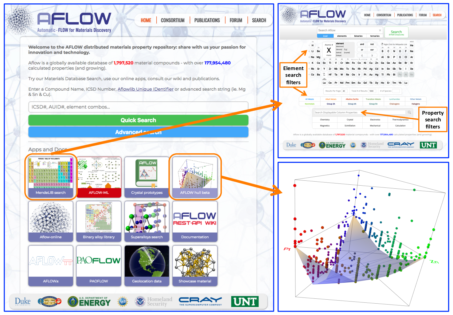
Figure 6: (a) Front page of the AFLOW online data repository, highlighting the link to (b) the AFLOW advanced search application, which facilitates complex search queries including filtering by chemical composition and materials properties and (c) the AFLOW interactive convex hull generator, showing the 3D hull for the Pt-Sc-Zn ternary alloy system.

Below are buttons linking to several different online applications such as the advanced search functionality, convex hull phase diagram generators, machine learning applications [45, 160, 161] and AFLOW-online data analysis tools. The link to the advanced search application is highlighted by the orange square, and the application page is shown in Figure 6(b). The advanced search application allows users to search for materials that contain (or exclude) specific elements or groups of elements, and also to filter and sort the results by properties such as electronic band structure energy gap (under the “Electronics” properties filter group) and bulk modulus (under the “Mechanical” properties filter group). This allows users to identify candidate materials with suitable materials properties for specific applications.

Another example online application available on the AFLOW web portal is the convex hull phase diagram generator. This application can be accessed by clicking on the button highlighted by the orange square in Figure 6(a), which will bring up a periodic table allowing users to select two or three elements for which they want to generate a convex hull. The application will then access the formation enthalpies and stoichiometries of the materials entries in the relevant alloy systems, and use this data to generate a two or three dimensional convex hull phase diagram as depicted in Figure 6(c). This application is fully interactive, allowing users to adjust the energy axis scale, rotate the diagram to view from different directions, and select specific points to obtain more information on the corresponding entries.

4.2 Programmatically accessible online repositories of computed materials properties

In order to use materials data in machine learning algorithms, it should be stored in a structured online database and made programmatically accessible via a representational state transfer API (REST-API). Examples of online repositories of materials data include AFLOW [4, 5], Materials Project [11], and OQMD [15]. There are also repositories that aggregate results from multiple sources such as NoMaD [23] and Citrine [162].

REST-APIs facilitate programmatic access to data repositories. Typical databases such as AFLOW are organized in layers, with the top layer corresponding to a project or catalog (e.g., binary alloys), the next layer corresponding to data sets (e.g., all of the entries for a particular alloy system), and then the bottom layer corresponding to specific materials entries, as illustrated in Figure 7(a).

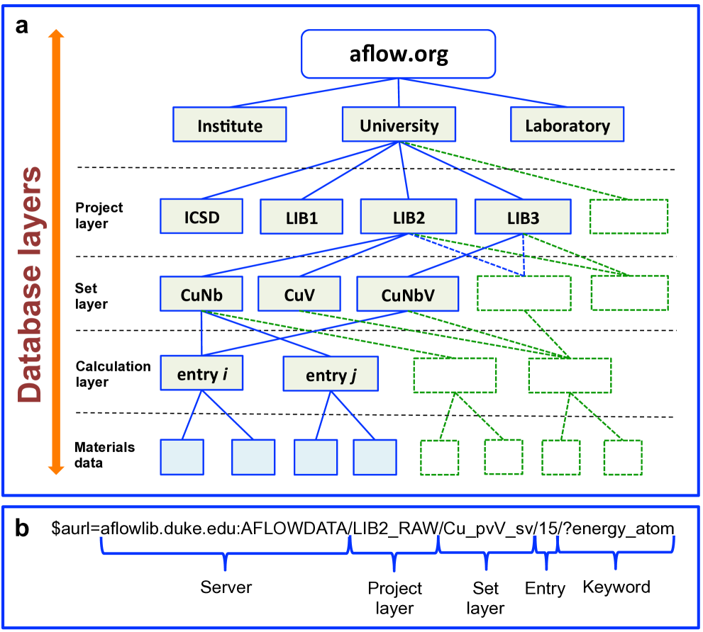
Figure 7: (a) The AFLOW database is organized as a multilayered system. (b) Example of an AURL which enables direct programmatic access to specific materials entry properties in the AFLOW database.

In the case of the AFLOW database, there are currently four different “projects”, namely the “ICSD”, “LIB1”, “LIB2” and “LIB3” projects; along with three more under construction: “LIB4”, “LIB5” and “LIB6”. The “ICSD” project contains calculated data for previously observed compounds [52], whereas the other three projects contain calculated data for single elements, binary alloys, and ternary alloys respectively, and are constructed by decorating prototype structures with combinations of different elements. Within “LIB2” and “LIB3”, there are many different data sets, each corresponding to a specific binary or ternary alloy system. Each entry in the set corresponds to a specific prototype structure and stoichiometry. The materials properties values for each of these entries are encoded via keywords, and the data can be accessed via URLs constructed from the different layer names and the appropriate keywords. In the case of the AFLOW database, the location of each layer and entry is identified by an AFLOW uniform resource locator (AURL) [5], which can be converted to a URL providing the absolute path to a particular layer, entry or property. The AURL takes the form server:AFLOWDATA/project/set/entry/?keywords, for example aflowlib.duke.edu:AFLOWDATA/LIB2_RAW/Cu_pvV_sv/15/?energy_atom, where aflowlib.duke.edu is the web address of the physical server where the data is located, LIB2_RAW is the binary alloy project layer, Cu_pvV_sv is the set containing the binary alloy system Cu-V, 15 is a specific entry with the composition Cu₃V in a tetragonal lattice, and energy_atom is the keyword corresponding to the property of energy per atom in units of eV, as shown in Figure 7(b). Each AURL can be converted to a web URL by changing the “:” after the server name to a “/”, so that the AURL in Figure 7(b) would become the URL aflowlib.duke.edu/AFLOWDATA/LIB2_RAW/Cu_pvV_sv/15/?energy_atom. This URL, if queried via a web browser or using a UNIX utility such as wget, returns the energy per atom in eV for entry 15 of the Cu-V binary alloy system.

In addition to the AURL, each entry in the AFLOW database is also associated with an AUID [5], which is a unique hexadecimal (base 16) number constructed from a checksum of the AFLOW output file for that entry. Since the AUID for a particular entry can always be reconstructed by applying the checksum procedure to the output file, it serves as a permanent, unique specifier for each calculation, irrespective of the current physical location of where the data are stored. This enables the retrieval of the results for a particular calculation from different servers, allowing for the construction of a truly distributed database that is robust against the failure or relocation of the physical hardware. Actual database versions can be identified from the version of AFLOW used to parse the calculation output files and postprocess the results to generate the database entry. This information can be retrieved using the keyword aflowlib_version.

The search and sort functions of the front-end portals can be combined with the programmatic data access functionality of the REST-API through the implementation of a Search-API. The AFLUX Search-API uses the LUX language to enable the embedding of logical operators within URL query strings [163]. For example, the energy per atom of every entry in the AFLOW repository containing the element Cu or V, but not the element Ti, with an electronic band gap between 2 and 5 eV, can be retrieved using the command: aflowlib.duke.edu/search/API/species((Cu:V),(!Ti)),Egap(2*,*5),energy_atom. In this AFLUX search query, the comma “,” represents the logical AND operation, the colon “:” the logical OR operation, the exclamation mark “!” the logical NOT operation, and the asterisk “*” is the “loose” operation that defines a range of values to search within. Note that by default AFLUX  returns only the first 64 entries matching the search query. The number and set of entries can be controlled by appending the paging directive to the end of the search query as follows: aflowlib.duke.edu/search/API/species((Cu:V),(!Ti)),Egap(2*,*5),energy_atom,paging(0), where calling the paging directive with the argument “0” instructs AFLUX to return all of the matching entries (note that this could potentially be a large amount of data, depending on the search query). The AFLUX Search-API allows users to construct and retrieve customized data sets, which they can feed into materials informatics machine learning packages to identify trends and correlations for use in rational materials design.

The use of APIs to provide programmatic access is being extended beyond materials data retrieval, to enable the remote use of pre-trained machine learning algorithms. The AFLOW-ML API [161] facilitates access to the two machine learning models that are also available online at aflow.org/aflow-ml [45, 160]. The API allows users to submit structural data for the material of interest using a utility such as cURL, and then returns the results of the model’s predictions in JSON format. The programmatic access to machine learning predictions enables the incorporation of machine learning into materials design workflows, allowing for rapid pre-screening to automatically select promising candidates for further investigation.

5 Materials applications

The automated approach to computational materials science has been used to accelerate the design of materials for structural applications such as metallic glasses and superalloys, and for functional applications including thermoelectrics, magnets, catalysts, batteries, photovoltaics and superconductors.

5.1 Disordered Materials

Section 2 describes how the thermodynamic stability of ordered compounds at zero temperature can be predicted from the convex hull phase diagrams generated using the formation enthalpies available in computational materials data repositories such as AFLOW [2, 4, 5, 6]. At finite temperature, however, entropic contributions due to thermally driven disorder play an important role, and lead to the formation of disordered materials such as metallic glasses and solid solutions. The thermodynamically favored phase at a given temperature and pressure is the phase with the lowest Gibbs free energy. Since the entropy term in the Gibbs free energy is multiplied by the temperature $T$, the entropic contribution to the Gibbs free energy becomes increasingly important at higher temperatures. The entropy of materials has two main components: the vibrational entropy, $S_{\begin{subarray}{c}\scalebox{0.6}{vib}\end{subarray}}$, which can be calculated from the phonon dispersion or the Debye model as described in Section 3; and the configuration entropy, $S_{\begin{subarray}{c}\scalebox{0.6}{config}\end{subarray}}$, due to the disorder in the atomic positions or site occupations. Configurational entropy originates from chemical disorder as in the case of high entropy alloys in which all of the atoms are arranged on a regular lattice, but the specific lattice sites are randomly occupied by different chemical species; or structural disorder as in the case of metallic glasses, where the atoms no longer occupy regular lattice sites resulting in an amorphous material.

High entropy materials. High entropy materials display structural order (i.e. all of the atoms are arranged on a periodic crystal lattice) but chemical disorder (i.e. the actual occupation of these lattice sites is random) [164].

In the ideal entropy limit in which the occupation of the atomic sites is completely random, the configuration entropy per atom is given by $S_{\begin{subarray}{c}\scalebox{0.6}{config}\end{subarray}}=k_{\begin{subarray}{c}\scalebox{0.6}{B}\end{subarray}}\sum_{i}x_{i}\log_{e}\left(x_{i}\right)$ [164], where $x_{i}$ is the fractional composition of each species component. Note that this expression increases with increasing numbers of species, and is also maximized when all of the values of $x_{i}$ are equal, i.e. for equimolar compositions.

The expression for the ideal entropy can be combined with calculations for special quasirandom structures (SQS) [165], which are special structural configurations where the radial correlation functions mimic those of a perfectly random structure, to estimate the Gibbs free energy for high entropy alloys. This can then be used in conjunction with the energies of the ordered phases obtained from computational materials data repositories such as AFLOW [2, 4, 5, 6] to generate structural phase diagrams as a function of temperature and composition, predicting the phase transition boundaries between ordered compounds, phase separation regions, and single phase solid solutions [108, 166, 167]. The calculated ordered structure energies in AFLOW can also be used to train cluster expansion models [168] to predict the energies of large ensembles of configurations, which can be combined with thermodynamic descriptors to estimate the transition temperature and miscibility gaps for solid solutions and high entropy alloys [169].

The concept of entropy stabilization has recently been extended beyond metallic alloys to include multi-component ceramics, such as high entropy oxides [170, 171]. High entropy oxides consist of an ordered anion sublattice occupied by oxygen ions, with a disordered cation sublattice randomly occupied by five different metal ions, such as Co, Cu, Mg, Ni and Zn [170, 171]. The oxygen ions screen the metal ions from each other, reducing the energy cost associated with forming a random configuration of the metal ions, enabling the formation of a single-phase, entropy-stabilized ceramic.

Metallic glasses. Metallic glasses are alloys in which the atoms do not occupy the sites of a regular periodic lattice, but instead form a structurally disordered amorphous phase. These materials are of great commercial and industrial interest due to their unique combination of superb mechanical properties [172] and plastic-like processability [173, 174, 175] for several potential applications [176, 177, 178, 179, 180].

Several different attempts have been made to understand the formation of metallic glasses and predict the glass forming ability (GFA) of different alloy compositions. Most of these efforts center around maximizing the packing density of the different atoms [181], which requires elements with a range of different atomic radii [182, 183, 184, 185, 186]. Other efforts have been made to use phase diagram data on liquidus temperatures to predict GFA [187, 188, 189]. Work is also underway to use machine learning techniques to predict potential glass formers [190].

Much of the theoretical work described above relies on the use of experimental rather than ab-initio computational data to predict new materials, due to the difficulty of modeling amorphous structures using first-principles techniques. However, Perim et al. [48] recently demonstrated that the energies of different structural phases can be combined into a descriptor to predict the formation of metallic glasses. If there are many different structural phases with similar formation enthalpy, this will frustrate crystallization during solidification and thus promote glass formation [48]. This frustration can be quantified to formulate a spectral descriptor for GFA using the structural and energetic information available in computational materials data repositories such as AFLOW [2, 4, 5, 6]. The differences in the geometry between two structures are quantified by describing each structure in terms of its atomic environments [191, 192, 193], while the formation enthalpy differences between the respective structures are expressed in the form of Boltzmann factors. The energetic and structural descriptors can then be combined with appropriate normalization factors to formulate a spectral descriptor for GFA as function of composition $x$: $GFA\left(\{x\}\right)$. Comparisons with known glass forming compositions available in the literature can then be used to define a threshold, such that if $GFA\left(\{x\}\right)$ exceeds this threshold, then the composition $x$ would be expected to be glass forming.

The $GFA\left(\{x\}\right)$ descriptor has been used to perform an automated analysis of the GFA of over 1,400 binary alloy systems from the AFLOW data repository [48]. While over half of all binary alloy systems are predicted to have a GFA below that of the threshold, nevertheless some 17% of alloy systems display a maximum value of $GFA\left(\{x\}\right)$ greater than the maximum value for the Cu-Zr system, a well-known good glass former. These included several alloy systems for which glass formation had never previously been observed or sometimes even investigated, suggesting that there are many possible glass forming compositions which remain to be discovered. This success demonstrates the power of combining descriptors based on the easily calculated properties of periodic crystalline phases with large pre-calculated databases for predicting the synthesizability of complex disordered materials.

Modeling off-stoichiometry materials. Incorporating the effects of disorder is a necessary, albeit difficult, step in materials modeling. Not only is disorder intrinsic to all materials, but it also offers a route to enhanced and even otherwise inaccessible functionality, as demonstrated by its ubiquity in technological applications. Prominent examples include fuel cells [194], high-temperature superconductors [195, 196], and low thermal conductivity thermoelectrics [197].

Specifically, chemical disorder can arise in the form of doping, vacancies, and even in the occupation of lattice sites themselves (random), which cannot inherently be modeled using periodic systems. One approach for modeling such effects includes SQS [165]. These quasirandom approximates are very computationally effective, but only offer a single representation of the disordered states, i.e., that with the lowest site correlations. Instead of reducing down to a single representation, AFLOW treats such systems as an ensemble of ordered supercells [198]. Properties are resolved through ensemble averages of the representative states, with opportunities to optimize computation (via supercell size/site error) and tune the level of disorder explored (via parameter $T$). AFLOW-POCC (AFLOW partial occupation module) has already resolved significant stoichiometric trends in wide-gap semiconductors and magnetic systems while offering additional insight into underlying physical mechanisms. Ultimately, the screening criteria and property predictions generated by these bona fide thermodynamic models and descriptors are accelerating design of new, technologically-significant materials, including advanced ceramics [199] and metallic glasses [48].

5.2 Superalloys

Superalloys are characterized by their extraordinary mechanical properties, particularly at temperatures near their melting point. Such traits make them the ideal candidates for applications in the aerospace and power generation industries. Among the more common examples, many have a face-centered cubic structure with base elements nickel, cobalt, and iron, though nickel-based superalloys dominate the market. Surprisingly, a novel cobalt-based superalloy, Co₃(Al,W) was discovered in 2006 that exhibits mechanical properties better than many nickel-based superalloys. This inspired a thorough computational investigation with AFLOW of alloys containing 40 different elements, yielding over 2,224 relevant ternary systems [59]. The search offered 102 systems shown to i. be more stable than Co₃[Al_0.5,W_0.5] — the L1₂-like random structure previously characterized thermodynamically [200] and very close to the compositions reported by experiments [201], ii. have a relevant concentration $\left(X_{3}[A_{x}B_{1-x}]\right)$ that is in two-phase equilibrium with the host matrix, and iii. exhibit only small deviations from the host matrix lattice (within 5% relative mismatch).

For these 102 candidates, additional pertinent properties were extracted, including the density and bulk modulus (as a proxy for hardness). Low density materials are preferred to mitigate the stress on turbine components. Significant trends for the bulk modulus are elucidated when plotting with respect to component $B$ on a Pettifor scale: Ni-based materials show a peak at or before Ni, whereas Co-based materials monotonically increase. Additionally, Co-based materials are generally more resistant to compression compared to Ni-based materials.

Of the 102 candidates, 37 materials have no reported phase diagrams in standard databases, and are thus expected to be unexplored or new. Additional screening based on the toxicity and (low) melting temperature of components uncovered six priority candidates for experimental validation.

5.3 Thermoelectrics

Thermoelectric materials generate an electric voltage when subjected to a temperature gradient, and can also generate a temperature gradient when a voltage is applied [202, 203]. Their lack of moving parts and resulting scalability means that they have potential applications in power generation for spacecraft, energy recovery from waste heat in automotive and industrial facilities [204, 205] and in spot cooling for nanoelectronics using the Peltier cooling effect [204, 205]. However, most of the available thermoelectric materials have low efficiency, only converting a few percent of the available thermal energy into electricity. Therefore, a major goal of thermoelectrics research is to develop new materials that have higher thermoelectric efficiency.

The thermoelectric efficiency of a material is determined by the figure of merit $zT$, which is obtained from [202, 203]

$$zT=\frac{\sigma{\sf S}^{2}T}{\kappa_{\begin{subarray}{c}\scalebox{0.6}{L}\end{subarray}}+\kappa_{\mathrm{e}}},$$ (35)

where S is the Seebeck coefficient, $\sigma$ is the electrical conductivity, $\kappa_{\begin{subarray}{c}\scalebox{0.6}{L}\end{subarray}}$ is the lattice thermal conductivity, and $\kappa_{\mathrm{e}}$ is the electronic thermal conductivity. The lattice thermal conductivity $\kappa_{\begin{subarray}{c}\scalebox{0.6}{L}\end{subarray}}$ can be calculated using the methods described in Section 3. Most of the electronic thermal conductivity $\kappa_{\mathrm{e}}$ will depend directly on the electrical conductivity $\sigma$ through the Wiedemann-Franz law [202]

$$\kappa_{\mathrm{e}}=L\sigma T,$$ (36)

where $L$ is the Lorenz factor, which has a value of $2.4\times 10^{-8}$ J² K^-2 C^-2 for free electrons. The Seebeck coefficient S is given by [202]

$${\sf S}=\frac{8\pi^{2}k_{\begin{subarray}{c}\scalebox{0.6}{B}\end{subarray}}^{2}}{3eh^{2}}m^{*}T\left(\frac{\pi}{3n}\right)^{\frac{2}{3}},$$ (37)

where $n$ is the charge carrier concentration, $e$ is the electronic charge, and $m^{*}$ is the density of states effective mass of the charge carriers in the material. The effective mass tensor $m_{ij}$ can be calculated from the curvature of electronic band structure dispersion $E(\vec{k})$

$$m_{ij}^{-1}=\frac{1}{\hbar^{2}}\frac{d^{2}E}{dk_{i}dk_{j}},$$ (38)

where $k_{i}$ and $k_{j}$ are components of the wave vector $\vec{k}$. Larger curvature of the band structure implies a lower effective mass, while flat narrow bands tend to result in a large effective mass. Charge carrier mobility and thus electrical conductivity tend to reduce with increasing effective mass. However, as can be seen from Equation 37, the Seebeck coefficient increases with effective mass, and $\kappa_{\mathrm{e}}$ also increases with $\sigma$. Therefore, a compromise should be found between high effective mass to maximize S and high charge carrier mobility to give high $\sigma$ in order to optimize the thermoelectric efficiency of the device.

Several computational high-throughput searches have been performed for thermoelectric materials [37, 38, 39, 40, 116, 206, 207, 208]. Many of the efforts towards developing more efficient thermoelectric materials have focused on either lowering the lattice thermal conductivity $\kappa_{\begin{subarray}{c}\scalebox{0.6}{L}\end{subarray}}$, or finding materials in which the electronic properties are highly directional, allowing for a narrow energy band distribution while simultaneously having a low effective mass, thus increasing the power factor $\sigma{\sf S}^{2}$. High-throughput searches for materials with low lattice thermal conductivity have focused on materials such as half-Heusler structures [39, 40, 209], which have lower densities and thus lower thermal conductivities than the full Heusler structures. Other promising materials include structures such as clathrates [210, 211, 212, 213, 214] and skutterudites [215, 216, 208, 217], which contain hollow voids that can be filled with “rattler” atoms to reduce the lattice thermal conductivity. Filled skutterudites in particular, such as $R_{x}$Co₄Sb₁₂, are excellent thermoelectric materials because of their combination of a high effective mass with high carrier mobility due to the existence of a secondary conduction band with 12 conducting charge carrier pockets [208].

Searches of large databases of inorganic materials to find new thermoelectrics include the study of 48,000 materials from the Materials Project database [206], where the power factor was calculated using the BoltzTraP code [218] and the thermal conductivity was estimated using the Clarke [219] and Cahill-Pohl [220] models. Almost 600 oxides, nitrides and sulfides from the ICSD were investigated by Garrity [116], where the lattice thermal conductivity was calculated at the quasiharmonic phonon level of approximation, with particular attention being paid to degeneracies in the conduction band minimum, or materials with strongly anisotropic conduction bands, that result in an effective low-dimensional conductor with a corresponding increase in the power factor. The thermoelectric material LiZnSb was proposed by an automated search of the calculated band structures of 1,640 compounds in the ICSD containing Sb [38], although later experimental measurements did not find a high thermoelectric efficiency for this compound [221].

Other strategies to increase the power factor include engineering the band structure [222] through volume changes by alloying different materials to create solid solutions, such as antifluorite Mg₂Si and Mg₂Ge with Mg₂Sn, or orthorhombic Ca₂Si and Ca₂Ge with Ca₂Sn [223]. Tuning the composition of alloys can also be used to converge the valence and conduction bands, enabling high valley degeneracy to be achieved in materials such as PbTe_1-xSe_x alloys [224]. Solid solutions can also produce local anisotropic structural disorder, increasing phonon scattering and thus improving the thermoelectric efficiency [225, 226].

The exploitation of thermodynamic phenomena such as spinodal decomposition to self-assemble heterostructures with increased phonon scattering [227] has also been proposed to enhance the efficiency of thermoelectric devices. In this approach, materials such as PbSe and PbTe, that are miscible at high temperatures, undergo phase separation when the mixture is cooled slowly, creating a layered heterostructure with a network of boundaries between the different components, which scatter phonons and thus suppress the thermal conductivity. This concept has also been extended to other nanotechnology applications, e.g. as a means to embed a network of electrically conducting nanowires, in the form of topologically protected interface states, within an insulating matrix [228].

The combination of different competing materials properties that must be optimized to maximize the thermoelectric efficiency highlights the importance of integrated frameworks such as AFLOW, which can automatically calculate different types of materials properties such as thermal conductivity and electronic band structures. Having all of these electronic and thermal properties calculated and available in an integrated, searchable, sortable data repository such as AFLOW.org accelerates the design of new, high-efficiency thermoelectric materials.

5.4 Magnetic materials

The search for new magnetic systems remains a longstanding challenge despite their ubiquity in modern technology [229]. Magnetism demonstrates remarkable sensitivity to a number of properties, including electronic configuration, bond length/angle, and magnetic ion valence, and thus its presence is rather uncommon and difficult to predict. In fact, only two percent of the known inorganic compounds [52] exhibit magnetic order of any kind. Consumer applications place additional practical restrictions for magnets, with the current global market effectively populated by only two dozen compounds. These obstacles motivated a large-scale computational search with AFLOW for new magnets among the Heusler structure family. Heusler structures are of particular interest for a number of reasons: i. several are known high-performance magnets, ii. the breadth of distinct compounds offers an excellent chance for discovery, iii. the full set of materials will likely offer other types of interesting materials (aside from magnets), and iv. they are metallic and thus well described by DFT. There are three types of Heusler structures, i.e., the regular- $X_{2}YZ$ (Cu₂MnAl-type), inverse- $\left(XY\right)XZ$ (Hg₂CuTi-type), and the half-Heuslers $XYZ$ (MgCuSb-type). By decorating these prototypes with ternary combinations of 55 elements, a total of 236,115 compounds were generated and added to the AFLOW.org repository.

As a first attempt, the analysis is limited to Heuslers containing elements of the 3$d$, 4$d$, and 5$d$ periods, i.e., a subset of 36,540 compounds. Of this set, 248 are determined to be thermodynamically stable and 22 have a magnetic ground state compatible with the unit cells considered. Among these 22 magnetic ground state compounds, a few prominent classes can be identified, including Co${}_{2}YZ$ and Mn${}_{2}YZ$. Upon further analysis of these classes, four materials became of particular interest. In the first class Co${}_{2}YZ$, there already exists 25 known compounds all lying on the Slater-Pauling curve (magnetic moment per formula unit versus number of valence electrons) [230]. The regression predicts Co₂MnTi to have the notably high Curie transition temperature $T_{\mathrm{C}}$ of 940 K — a feature shared by only two dozen known magnets. The second class Mn${}_{2}YZ$ is of interest because of their high $T_{\mathrm{C}}$ and potentially large magnetocrystalline anisotropy [231]. Two known examples from this class, Mn₂VAl and Mn₂VGa, show ferrimagnetic ordering, matching two candidates from the list of 22, Mn₂PtCo and Mn₂PtV. One more compound was highlighted for satisfying a stringent thermodynamic constraint. Mn₂PdPt shows to be robustly stable by at least 30 meV, where the criterion derives from the distance of the stable phase from the pseudo convex hull that neglects it. This criterion quantifies the impact of the structure on the minimum energy surface.

Following an attempt to synthesis these four candidates, two were successful (Co₂MnTi and Mn₂PtPd) and the other two decomposed into binary compounds. In fact, Co₂MnTi shows a $T_{\mathrm{C}}$ of 938 K, almost exactly as predicted by the Slater-Pauling curve. Surprisingly, Mn₂PdPt shows antiferromagnetic ordering and tetragonal distortion ($c/a\sim 1.8$), a result corroborated by calculation upon further analysis. Beyond the synthesis of these two systems, this investigation offers a new, accelerated pathway to discovery over traditional trial-and-error approaches.

6 Conclusion

Automated computational materials design frameworks have the capability to rapidly generate materials data without the need for laborious human intervention. They are being used to construct large repositories of programmatically accessible materials properties, calculated in a standardized, consistent fashion so as to facilitate the identification of trends and the training of machine learning models to predict electronic, thermal and mechanical behavior. When combined with physical models and intelligently formulated descriptors, the data becomes a powerful tool to accelerate the discovery of new materials for applications ranging from high-temperature superalloys to thermoelectrics and magnets.

7 Acknowledgments

We thank Drs. S. Barzilai, Y. Lederer, O. Levy, F. Rose, P. Nath, D. Usanmaz, D. Hicks, E. Gossett, D. Ford, R. Friedrich, M. Esters, P. Colinet, E. Perim, C. Calderon, K. Yang, M. Mehl, M. Buongiorno Nardelli, M. Fornari, G. Hart, I. Takeuchi, E. Zurek, P. Avery, R. Hanson, A. Kolmogorov, A. Natan, N. Mingo, J. Carrete, S. Sanvito, D. Brenner, K. Vecchio, M. Scheffler, L. Ghiringhelli, O. Isayev, A. Tropsha, J. Schroers and J. J. Vlassak for insightful discussions. This work is supported by DOD-ONR (N00014-16-1-2326, N00014-16-1-2583, N00014-17-1-2090, N00014-17-1-2876), by NSF (DMR-1436151), and by the Duke University—Center for Materials Genomics. SC acknowledges support by the Alexander von Humboldt-Foundation for financial support. CO acknowledges support from the NSF Graduate Research Fellowship #DGF1106401.

References

- [1] S. Curtarolo, G. L. W. Hart, M. Buongiorno Nardelli, N. Mingo, S. Sanvito, and O. Levy, The high-throughput highway to computational materials design, Nat. Mater. 12, 191–201 (2013).
- [2] S. Curtarolo, W. Setyawan, G. L. W. Hart, M. Jahnátek, R. V. Chepulskii, R. H. Taylor, S. Wang, J. Xue, K. Yang, O. Levy, M. J. Mehl, H. T. Stokes, D. O. Demchenko, and D. Morgan, AFLOW: An automatic framework for high-throughput materials discovery, Comput. Mater. Sci. 58, 218–226 (2012).
- [3] W. Setyawan and S. Curtarolo, High-throughput electronic band structure calculations: Challenges and tools, Comput. Mater. Sci. 49, 299–312 (2010).
- [4] S. Curtarolo, W. Setyawan, S. Wang, J. Xue, K. Yang, R. H. Taylor, L. J. Nelson, G. L. W. Hart, S. Sanvito, M. Buongiorno Nardelli, N. Mingo, and O. Levy, AFLOWLIB.ORG: A distributed materials properties repository from high-throughput ab initio calculations, Comput. Mater. Sci. 58, 227–235 (2012).
- [5] R. H. Taylor, F. Rose, C. Toher, O. Levy, K. Yang, M. Buongiorno Nardelli, and S. Curtarolo, A RESTful API for exchanging materials data in the AFLOWLIB.org consortium, Comput. Mater. Sci. 93, 178–192 (2014).
- [6] C. E. Calderon, J. J. Plata, C. Toher, C. Oses, O. Levy, M. Fornari, A. Natan, M. J. Mehl, G. L. W. Hart, M. Buongiorno Nardelli, and S. Curtarolo, The AFLOW standard for high-throughput materials science calculations, Comput. Mater. Sci. 108 Part A, 233–238 (2015).
- [7] W. Setyawan and S. Curtarolo, AflowLib: Ab-initio Electronic Structure Library Database, http://www.aflow.org (2011).
- [8] C. Toher, C. Oses, D. Hicks, E. Gossett, F. Rose, P. Nath, D. Usanmaz, D. C. Ford, E. Perim, C. E. Calderon, J. J. Plata, Y. Lederer, M. Jahnátek, W. Setyawan, S. Wang, J. Xue, K. Rasch, R. V. Chepulskii, R. H. Taylor, G. Gomez, H. Shi, A. R. Supka, R. Al Rahal Al Orabi, P. Gopal, F. T. Cerasoli, L. Liyanage, H. Wang, I. Siloi, L. A. Agapito, C. Nyshadham, G. L. W. Hart, J. Carrete, F. Legrain, N. Mingo, E. Zurek, O. Isayev, A. Tropsha, S. Sanvito, R. M. Hanson, I. Takeuchi, M. J. Mehl, A. N. Kolmogorov, K. Yang, P. D’Amico, A. Calzolari, M. Costa, R. De Gennaro, M. Buongiorno Nardelli, M. Fornari, O. Levy, and S. Curtarolo, The AFLOW Fleet for Materials Discovery, vol. arXiv:1712.00422 (2018).
- [9] A. R. Supka, T. E. Lyons, L. S. I. Liyanage, P. D’Amico, R. Al Rahal Al Orabi, S. Mahatara, P. Gopal, C. Toher, D. Ceresoli, A. Calzolari, S. Curtarolo, M. Buongiorno Nardelli, and M. Fornari, AFLOW: A minimalist approach to high-throughput ab initio calculations including the generation of tight-binding hamiltonians, Comput. Mater. Sci. 136, 76–84 (2017).
- [10] M. Buongiorno Nardelli, F. T. Cerasoli, M. Costa, S. Curtarolo, R. De Gennaro, M. Fornari, L. Liyanage, A. R. Supka, and H. Wang, PAOFLOW: A utility to construct and operate on ab initio Hamiltonians from the projections of electronic wavefunctions on atomic orbital bases, including characterization of topological materials, Comput. Mater. Sci. 143, 462–472 (2017).
- [11] A. Jain, G. Hautier, C. J. Moore, S. P. Ong, C. C. Fischer, T. Mueller, K. A. Persson, and G. Ceder, A high-throughput infrastructure for density functional theory calculations, Comput. Mater. Sci. 50, 2295–2310 (2011).
- [12] A. Jain, S. P. Ong, G. Hautier, W. Chen, W. D. Richards, S. Dacek, S. Cholia, D. Gunter, D. Skinner, G. Ceder, and K. A. Persson, Commentary: The Materials Project: A materials genome approach to accelerating materials innovation, APL Mater. 1, 011002 (2013).
- [13] S. P. Ong, W. D. Richards, A. Jain, G. Hautier, M. Kocher, S. Cholia, D. Gunter, V. L. Chevrier, K. A. Persson, and G. Ceder, Python Materials Genomics (pymatgen): A robust, open-source python library for materials analysis, Comput. Mater. Sci. 68, 314–319 (2013).
- [14] K. Mathew, J. H. Montoya, A. Faghaninia, S. Dwarakanath, M. Aykol, H. Tang, I. Chu, T. Smidt, B. Bocklund, M. Horton, J. Dagdelen, B. Wood, Z.-K. Liu, J. Neaton, S. P. Ong, K. A. Persson, and A. Jain, Atomate: A high-level interface to generate, execute, and analyze computational materials science workflows, Comput. Mater. Sci. 139, 140–152 (2017).
- [15] J. E. Saal, S. Kirklin, M. Aykol, B. Meredig, and C. Wolverton, Materials Design and Discovery with High-Throughput Density Functional Theory: The Open Quantum Materials Database (OQMD), JOM 65, 1501–1509 (2013).
- [16] S. Kirklin, B. Meredig, and C. Wolverton, High-Throughput Computational Screening of New Li-Ion Battery Anode Materials, Adv. Energy Mater. 3, 252–262 (2013).
- [17] S. Kirklin, J. E. Saal, V. I. Hegde, and C. Wolverton, High-throughput computational search for strengthening precipitates in alloys, Acta Mater. 102, 125–135 (2016).
- [18] D. D. Landis, J. S. Hummelshøj, S. Nestorov, J. Greeley, M. Dułak, T. Bligaard, J. K. Nørskov, and K. W. Jacobsen, The Computational Materials Repository, Comput. Sci. Eng. 14, 51–57 (2012).
- [19] S. R. Bahn and K. W. Jacobsen, An object-oriented scripting interface to a legacy electronic structure code, Comput. Sci. Eng. 4, 56–66 (2002).
- [20] G. Pizzi, A. Cepellotti, R. Sabatini, N. Marzari, and B. Kozinsky, AiiDA, http://www.aiida.net (2016).
- [21] G. Pizzi, A. Cepellotti, R. Sabatini, N. Marzari, and B. Kozinsky, AiiDA: automated interactive infrastructure and database for computational science, Comput. Mater. Sci. 111, 218–230 (2016).
- [22] N. Mounet, M. Gibertini, P. Schwaller, D. Campi, A. Merkys, A. Marrazzo, T. Sohier, I. E. Castelli, A. Cepellotti, G. Pizzi, and N. Marzari, Two-dimensional materials from high-throughput computational exfoliation of experimentally known compounds, Nat. Nanotechnol. 13, 246–252 (2018).
- [23] M. Scheffler, C. Draxl, and Computer Center of the Max-Planck Society, Garching, The NoMaD Repository, http://nomad-repository.eu (2014).
- [24] A. Merkys, N. Mounet, A. Cepellotti, N. Marzari, S. Graz̆ulis, and G. Pizzi, A posteriori metadata from automated provenance tracking: integration of AiiDA and TCOD, J. Cheminform. 9, 56 (2017).
- [25] L. Yu and A. Zunger, Identification of Potential Photovoltaic Absorbers Based on First-Principles Spectroscopic Screening of Materials, Phys. Rev. Lett. 108, 068701 (2012).
- [26] I. E. Castelli, T. Olsen, S. Datta, D. D. Landis, S. Dahl, K. S. Thygesen, and K. W. Jacobsen, Computational screening of perovskite metal oxides for optimal solar light capture, Energy Environ. Sci. 5, 5814–5819 (2012).
- [27] L.-C. Lin, A. H. Berger, R. L. Martin, J. Kim, J. A. Swisher, K. Jariwala, C. H. Rycroft, A. S. Bhown, M. W. Deem, M. Haranczyk, and B. Smit, In silico screening of carbon-capture materials, Nat. Mater. 11, 633–641 (2012).
- [28] S. V. Alapati, J. K. Johnson, and D. S. Sholl, Large-Scale Screening of Metal Hydride Mixtures for High-Capacity Hydrogen Storage from First-Principles Calculations, J. Phys. Chem. C 112, 5258–5262 (2008).
- [29] S. Derenzo, G. Bizarri, R. Borade, E. Bourret-Courchesne, R. Boutchko, A. Canning, A. Chaudhry, Y. Eagleman, G. Gundiah, S. Hanrahan, M. Janecek, and M. Weber, New scintillators discovered by high-throughput screening, Nuclear Inst. and Methods in Physics Research, A 652, 247–250 (2011).
- [30] C. Ortiz, O. Eriksson, and M. Klintenberg, Data mining and accelerated electronic structure theory as a tool in the search for new functional materials, Comput. Mater. Sci. 44, 1042–1049 (2009).
- [31] W. Setyawan, R. M. Gaumé, S. Lam, R. S. Feigelson, and S. Curtarolo, High-Throughput Combinatorial Database of Electronic Band Structures for Inorganic Scintillator Materials, ACS Comb. Sci. 13, 382–390 (2011).
- [32] W. Setyawan, R. M. Gaumé, R. S. Feigelson, and S. Curtarolo, Comparative Study of Nonproportionality and Electronic Band Structures Features in Scintillator Materials, IEEE Trans. Nucl. Sci. 56, 2989–2996 (2009).
- [33] K. Yang, W. Setyawan, S. Wang, M. Buongiorno Nardelli, and S. Curtarolo, A search model for topological insulators with high-throughput robustness descriptors, Nat. Mater. 11, 614–619 (2012).
- [34] H. Lin, L. A. Wray, Y. Xia, S. Xu, S. Jia, R. J. Cava, A. Bansil, and M. Z. Hasan, Half-Heusler ternary compounds as new multifunctional experimental platforms for topological quantum phenomena, Nat. Mater. 9, 546–549 (2010).
- [35] R. Armiento, B. Kozinsky, M. Fornari, and G. Ceder, Screening for high-performance piezoelectrics using high-throughput density functional theory, Phys. Rev. B 84, 014103 (2011).
- [36] A. Roy, J. W. Bennett, K. M. Rabe, and D. Vanderbilt, Half-Heusler Semiconductors as Piezoelectrics, Phys. Rev. Lett. 109, 037602 (2012).
- [37] S. Wang, Z. Wang, W. Setyawan, N. Mingo, and S. Curtarolo, Assessing the Thermoelectric Properties of Sintered Compounds via High-Throughput Ab-Initio Calculations, Phys. Rev. X 1, 021012 (2011).
- [38] G. K. H. Madsen, Automated Search for New Thermoelectric Materials: The Case of LiZnSb, J. Am. Chem. Soc. 128, 12140–12146 (2006).
- [39] J. Carrete, W. Li, N. Mingo, S. Wang, and S. Curtarolo, Finding Unprecedentedly Low-Thermal-Conductivity Half-Heusler Semiconductors via High-Throughput Materials Modeling, Phys. Rev. X 4, 011019 (2014).
- [40] J. Carrete, N. Mingo, S. Wang, and S. Curtarolo, Nanograined Half-Heusler Semiconductors as Advanced Thermoelectrics: An Ab Initio High-Throughput Statistical Study, Adv. Func. Mater. 24, 7427–7432 (2014).
- [41] J. K. Nørskov, T. Bligaard, J. Rossmeisel, and C. H. Christensen, Towards the computational design of solid catalysts, Nat. Chem. 1, 37 (2009).
- [42] G. Hautier, A. Jain, H. Chen, C. Moore, S. P. Ong, and G. Ceder, Novel mixed polyanions lithium-ion batery cathode materials predicted by high-throughput ab initio computations, J. Mater. Chem. 21, 17147–17153 (2011).
- [43] G. Hautier, A. Jain, S. P. Ong, B. Kang, C. Moore, R. Doe, and G. Ceder, Phosphates as Lithium-Ion Battery Cathodes: An Evaluation Based on High-Throughput ab Initio Calculations, Chem. Mater. 23, 3495–3508 (2011).
- [44] T. Mueller, G. Hautier, A. Jain, and G. Ceder, Evaluation of Tavorite-Structured Cathode Materials for Lithium-Ion Batteries Using High-Throughput Computing, Chem. Mater. 23, 3854–3862 (2011).
- [45] O. Isayev, C. Oses, C. Toher, E. Gossett, S. Curtarolo, and A. Tropsha, Universal fragment descriptors for predicting electronic properties of inorganic crystals, Nat. Commun. 8, 15679 (2017).
- [46] M. de Jong, W. Chen, R. Notestine, K. A. Persson, G. Ceder, A. Jain, M. D. Asta, and A. Gamst, A Statistical Learning Framework for Materials Science: Application to Elastic Moduli of -nary Inorganic Polycrystalline Compounds, Sci. Rep. 6, 34256 (2016).
- [47] O. Isayev, D. Fourches, E. N. Muratov, C. Oses, K. Rasch, A. Tropsha, and S. Curtarolo, Materials Cartography: Representing and Mining Materials Space Using Structural and Electronic Fingerprints, Chem. Mater. 27, 735–743 (2015).
- [48] E. Perim, D. Lee, Y. Liu, C. Toher, P. Gong, Y. Li, W. N. Simmons, O. Levy, J. J. Vlassak, J. Schroers, and S. Curtarolo, Spectral descriptors for bulk metallic glasses based on the thermodynamics of competing crystalline phases, Nat. Commun. 7, 12315 (2016).
- [49] C. Toher, J. J. Plata, O. Levy, M. de Jong, M. D. Asta, M. Buongiorno Nardelli, and S. Curtarolo, High-throughput computational screening of thermal conductivity, Debye temperature, and Grüneisen parameter using a quasiharmonic Debye model, Phys. Rev. B 90, 174107 (2014).
- [50] M. de Jong, W. Chen, T. Angsten, A. Jain, R. Notestine, A. Gamst, M. Sluiter, C. K. Ande, S. van der Zwaag, J. J. Plata, C. Toher, S. Curtarolo, G. Ceder, K. A. Persson, and M. D. Asta, Charting the Complete Elastic properties of Inorganic Crystalline Compounds, Sci. Data 2, 150009 (2015).
- [51] C. Toher, C. Oses, J. J. Plata, D. Hicks, F. Rose, O. Levy, M. de Jong, M. D. Asta, M. Fornari, M. Buongiorno Nardelli, and S. Curtarolo, Combining the AFLOW GIBBS and Elastic Libraries to efficiently and robustly screen thermomechanical properties of solids, Phys. Rev. Mater. 1, 015401 (2017).
- [52] G. Bergerhoff, R. Hundt, R. Sievers, and I. D. Brown, The inorganic crystal structure data base, J. Chem. Inf. Comput. Sci. 23, 66–69 (1983).
- [53] M. J. Mehl, Naval Research Laboratory Crystal Structure database, http://cst-www.nrl.navy.mil/lattice/ (2011).
- [54] M. J. Mehl, D. Hicks, C. Toher, O. Levy, R. M. Hanson, G. L. W. Hart, and S. Curtarolo, The AFLOW Library of Crystallographic Prototypes: Part 1, Comput. Mater. Sci. 136, S1–S828 (2017).
- [55] G. L. W. Hart and R. W. Forcade, Algorithm for generating derivative structures, Phys. Rev. B 77, 224115 (2008).
- [56] G. L. W. Hart and R. W. Forcade, Generating derivative structures from multilattices: Algorithm and application to hcp alloys, Phys. Rev. B 80, 014120 (2009).
- [57] S. Curtarolo, D. Morgan, and G. Ceder, Accuracy of ab initio methods in predicting the crystal structures of metals: A review of 80 binary alloys, Calphad 29, 163–211 (2005).
- [58] G. L. W. Hart, S. Curtarolo, T. B. Massalski, and O. Levy, Comprehensive Search for New Phases and Compounds in Binary Alloy Systems Based on Platinum-Group Metals, Using a Computational First-Principles Approach, Phys. Rev. X 3, 041035 (2013).
- [59] C. Nyshadham, C. Oses, J. E. Hansen, I. Takeuchi, S. Curtarolo, and G. L. W. Hart, A computational high-throughput search for new ternary superalloys, Acta Mater. 122, 438–447 (2017).
- [60] S. P. Ong, L. Wang, B. Kang, and G. Ceder, Li-Fe-P-O2 Phase Diagram from First Principles Calculations, Chem. Mater. 20, 1798–1807 (2008).
- [61] A. R. Akbarzadeh, V. Ozoliņš, and C. Wolverton, First-principles determination of multicomponent hydride phase diagrams: Application to the Li-Mg-N-H system, Adv. Mater. 19, 3233–3239 (2007).
- [62] O. Levy, G. L. W. Hart, and S. Curtarolo, Uncovering Compounds by Synergy of Cluster Expansion and High-Throughput Methods, J. Am. Chem. Soc. 132, 4830–4833 (2010).
- [63] O. Levy, G. L. W. Hart, and S. Curtarolo, Hafnium binary alloys from experiments and first principles, Acta Mater. 58, 2887–2897 (2010).
- [64] O. Levy, R. V. Chepulskii, G. L. W. Hart, and S. Curtarolo, The New face of Rhodium Alloys: Revealing Ordered Structures from First Principles, J. Am. Chem. Soc. 132, 833–837 (2010).
- [65] O. Levy, M. Jahnátek, R. V. Chepulskii, G. L. W. Hart, and S. Curtarolo, Ordered Structures in Rhenium Binary Alloys from First-Principles Calculations, J. Am. Chem. Soc. 133, 158–163 (2011).
- [66] M. Jahnátek, O. Levy, G. L. W. Hart, L. J. Nelson, R. V. Chepulskii, J. Xue, and S. Curtarolo, Ordered phases in ruthenium binary alloys from high-throughput first-principles calculations, Phys. Rev. B 84, 214110 (2011).
- [67] O. Levy, J. Xue, S. Wang, G. L. W. Hart, and S. Curtarolo, Stable ordered structures of binary technetium alloys from first principles, Phys. Rev. B 85, 012201 (2012).
- [68] R. V. Chepulskii and S. Curtarolo, Revealing low-temperature atomic ordering in bulk Co-Pt with the high-throughput ab-initio method, Appl. Phys. Lett. 99, 261902 (2011).
- [69] R. H. Taylor, S. Curtarolo, and G. L. W. Hart, Ordered magnesium-lithium alloys: First-principles predictions, Phys. Rev. B 81, 024112 (2010).
- [70] R. H. Taylor, S. Curtarolo, and G. L. W. Hart, Guiding the experimental discovery of magnesium alloys, Phys. Rev. B 84, 084101 (2011).
- [71] R. V. Chepulskii and S. Curtarolo, Calculation of solubility in titanium alloys from first principles, Acta Mater. 57, 5314 (2009).
- [72] J. Bloch, O. Levy, B. Pejova, J. Jacob, S. Curtarolo, and B. Hjörvarsson, Prediction and Hydrogen Acceleration of Ordering in Iron-Vanadium Alloys, Phys. Rev. Lett. 108, 215503 (2012).
- [73] M. J. Mehl, D. Finkenstadt, C. Dane, G. L. W. Hart, and S. Curtarolo, Finding the stable structures of N1-xWx with an ab initio high-throughput approach, Phys. Rev. B 91, 184110 (2015).
- [74] O. Levy, G. L. W. Hart, and S. Curtarolo, Structure maps for hcp metals from first-principles calculations, Phys. Rev. B 81, 174106 (2010).
- [75] R. H. Taylor, S. Curtarolo, and G. L. W. Hart, Predictions of the Pt8Ti Phase in Unexpected Systems, J. Am. Chem. Soc. 132, 6851–6854 (2010).
- [76] L. J. Nelson, G. L. W. Hart, and S. Curtarolo, Ground-state characterizations of systems predicted to exhibit L11 or L13 crystal structures, Phys. Rev. B 85, 054203 (2012).
- [77] P. Hohenberg and W. Kohn, Inhomogeneous Electron Gas, Phys. Rev. 136, B864–B871 (1964).
- [78] W. Kohn and L. J. Sham, Self-consistent equations including exchange and correlation effects, Phys. Rev. 140, A1133 (1965).
- [79] J. P. Perdew and A. Zunger, Self-interaction correction to density-functional approximations for many-electron systems, Phys. Rev. B 23, 5048–5079 (1981).
- [80] A. Zupan, P. Blaha, K. Schwarz, and J. P. Perdew, Pressure-induced phase transitions in solid Si, SiO2, and Fe: Performance of local-spin-density and generalized-gradient-approximation density functionals, Phys. Rev. B 58, 11266 (1998).
- [81] J. P. Perdew, K. Burke, and M. Ernzerhof, Generalized Gradient Approximation Made Simple, Phys. Rev. Lett. 77, 3865–3868 (1996).
- [82] C. Lee, W. Yang, and R. G. Parr, Development of the Colle-Salvetti correlation-energy formula into a functional of the electron density, Phys. Rev. B 37, 785 (1988).
- [83] J. Sun, A. Ruzsinszky, and J. P. Perdew, Strongly Constrained and Appropriately Normed Semilocal Density Functional, Phys. Rev. Lett. 115, 036402 (2015).
- [84] A. I. Liechtenstein, V. I. Anisimov, and J. Zaanen, Density-functional theory and strong interactions: Orbital ordering in Mott-Hubbard insulators, Phys. Rev. B 52, R5467 (1995).
- [85] S. L. Dudarev, G. A. Botton, S. Y. Savrasov, C. J. Humphreys, and A. P. Sutton, Electron-energy-loss spectra and the structural stability of nickel oxide: An LSDA study, Phys. Rev. B 57, 1505–1509 (1998).
- [86] A. D. Becke, Density-functional thermochemistry. III. The role of exact exchange, J. Chem. Phys. 98, 5648 (1993).
- [87] J. Heyd, G. E. Scuseria, and M. Ernzerhof, Hybrid functionals based on a screened Coulomb potential, J. Chem. Phys. 118, 8207–8215 (2003).
- [88] L. A. Agapito, S. Curtarolo, and M. Buongiorno Nardelli, Reformulation of as a Pseudohybrid Hubbard Density Functional for Accelerated Materials Discovery, Phys. Rev. X 5, 011006 (2015).
- [89] L. Hedin, New Method for Calculating the One-Particle Green’s Function with Application to the Electron-Gas Problem, Phys. Rev. 139, A796–A823 (1965).
- [90] F. Aryasetiawan and O. Gunnarsson, The Method, Rep. Prog. Phys. 61, 237 (1998).
- [91] G. Kresse and J. Hafner, Ab initio molecular dynamics for liquid metals, Phys. Rev. B 47, 558–561 (1993).
- [92] G. Kresse and J. Furthmüller, Efficient iterative schemes for ab initio total-energy calculations using a plane-wave basis set, Phys. Rev. B 54, 11169–11186 (1996).
- [93] G. Kresse and J. Furthmüller, Efficiency of ab-initio total energy calculations for metals and semiconductors using a plane-wave basis set, Comput. Mater. Sci. 6, 15–50 (1996).
- [94] G. Kresse and D. Joubert, From ultrasoft pseudopotentials to the projector augmented-wave method, Phys. Rev. B 59, 1758–1775 (1999).
- [95] P. Giannozzi, S. Baroni, N. Bonini, M. Calandra, R. Car, C. Cavazzoni, D. Ceresoli, G. L. Chiarotti, M. Cococcioni, I. Dabo, A. Dal Corso, S. de Gironcoli, S. Fabris, G. Fratesi, R. Gebauer, U. Gerstmann, C. Gougoussis, A. Kokalj, M. Lazzeri, L. Martin-Samos, N. Marzari, F. Mauri, R. Mazzarello, S. Paolini, A. Pasquarello, L. Paulatto, C. Sbraccia, S. Scandolo, G. Sclauzero, A. P. Seitsonen, A. Smogunov, P. Umari, and R. M. Wentzcovitch, QUANTUM ESPRESSO: a modular and open-source software project for quantum simulations of materials, J. Phys.: Condens. Matter 21, 395502 (2009).
- [96] P. Giannozzi, O. Andreussi, T. Brumme, O. Bunau, M. Buongiorno Nardelli, M. Calandra, R. Car, C. Cavazzoni, D. Ceresoli, M. Cococcioni, N. Colonna, I. Carnimeo, A. Dal Corso, S. de Gironcoli, P. Delugas, R. A. DiStasio Jr., A. Ferretti, A. Floris, G. Fratesi, G. Fugallo, R. Gebauer, U. Gerstmann, F. Giustino, T. Gorni, J. Jia, M. Kawamura, H.-Y. Ko, A. Kokalj, E. Küçükbenli, M. Lazzeri, M. Marsili, N. Marzari, F. Mauri, N. L. Nguyen, H.-V. Nguyen, A. Otero-de-la-Roza, L. Paulatto, S. Poncé, D. Rocca, R. Sabatini, B. Santra, M. Schlipf, A. P. Seitsonen, A. Smogunov, I. Timrov, T. Thonhauser, P. Umari, N. Vast, X. Wu, and S. Baroni, Advanced capabilities for materials modelling with Quantum ESPRESSO, J. Phys.: Condens. Matter 29, 465901 (2017).
- [97] X. Gonze, J. M. Beuken, R. Caracas, F. Detraux, M. Fuchs, G. M. Rignanese, L. Sindic, M. Verstraete, G. Zerah, F. Jollet, M. Torrent, A. Roy, M. Mikami, P. Ghosez, J. Y. Raty, and D. C. Allan, First-principles computation of material properties: the ABINIT software project, Comput. Mater. Sci. 25, 478–492 (2002).
- [98] X. Gonze, B. Amadon, P.-M. Anglade, J.-M. Beuken, F. Bottin, P. Boulanger, F. Bruneval, D. Caliste, R. Caracas, M. Côté, T. Deutsch, L. Genovese, P. Ghosez, M. Giantomassi, S. Goedecker, D. R. Hamann, P. Hermet, F. Jollet, G. Jomard, S. Leroux, M. Mancini, S. Mazevet, M. J. T. Oliveira, G. Onida, Y. Pouillon, T. Rangel, G.-M. Rignanese, D. Sangalli, R. Shaltaf, M. Torrent, M. J. Verstraete, G. Zerah, and J. W. Zwanziger, ABINIT: First-principles approach to materials and nanosystem properties, Comput. Phys. Commun. 180, 2582–2615 (2009).
- [99] V. Blum, R. Gehrke, F. Hanke, P. Havu, V. Havu, X. Ren, K. Reuter, and M. Scheffler, Ab initio molecular simulations with numeric atom-centered orbitals, Comput. Phys. Commun. 180, 2175–2196 (2009).
- [100] J. M. Soler, E. Artacho, J. D. Gale, A. García, J. Junquera, P. Ordejón, and D. Sánchez-Portal, The SIESTA method for ab initio order-N materials simulation, J. Phys.: Condens. Matter 14, 2745 (2002).
- [101] M. J. Frisch, G. W. Trucks, H. B. Schlegel, G. E. Scuseria, M. A. Robb, J. R. Cheeseman, G. Scalmani, V. Barone, B. Mennucci, G. A. Petersson, H. Nakatsuji, M. Caricato, X. Li, H. P. Hratchian, A. F. Izmaylov, J. Bloino, G. Zheng, J. L. Sonnenberg, M. Hada, M. Ehara, K. Toyota, R. Fukuda, J. Hasegawa, M. Ishida, T. Nakajima, Y. Honda, O. Kitao, H. Nakai, T. Vreven, J. A. Montgomery Jr., J. E. Peralta, F. Ogliaro, M. Bearpark, J. J. Heyd, E. Brothers, K. N. Kudin, V. N. Staroverov, R. Kobayashi, J. Normand, K. Raghavachari, A. Rendell, J. C. Burant, S. S. Iyengar, J. Tomasi, M. Cossi, N. Rega, J. M. Millam, M. Klene, J. E. Knox, J. B. Cross, V. Bakken, C. Adamo, J. Jaramillo, R. Gomperts, R. E. Stratmann, O. Yazyev, A. J. Austin, R. Cammi, C. Pomelli, J. W. Ochterski, R. L. Martin, K. Morokuma, V. G. Zakrzewski, G. A. Voth, P. Salvador, J. J. Dannenberg, S. Dapprich, A. D. Daniels, O. Farkas, J. B. Foresman, J. V. Ortiz, J. Cioslowski, and D. J. Fox, Gaussian09 Revision D.01. Gaussian Inc. Wallingford CT 2009.
- [102] W. J. Hehre, R. F. Stewart, and J. A. Pople, Self-Consistent Molecular-Orbital Methods. I. Use of Gaussian Expansions of Slater-Type Atomic Orbitals, J. Chem. Phys. 51, 2657–2664 (1969).
- [103] H. J. Monkhorst and J. D. Pack, Special points for Brillouin-zone integrations, Phys. Rev. B 13, 5188 (1976).
- [104] P. Wisesa, K. A. McGill, and T. Mueller, Efficient generation of generalized Monkhorst-Pack grids through the use of informatics, Phys. Rev. B 93, 155109 (2016).
- [105] G. N. Greaves, A. L. Greer, R. S. Lakes, and T. Rouxel, Poisson’s ratio and modern materials, Nat. Mater. 10, 823–837 (2011).
- [106] J.-P. Poirier, Introduction to the Physics of the Earth’s Interior (Cambridge University Press, 2000), 2nd edn.
- [107] F. Mouhat and F.-X. Coudert, Necessary and sufficient elastic stability conditions in various crystal systems, Phys. Rev. B 90, 224104 (2014).
- [108] S. Barzilai, C. Toher, S. Curtarolo, and O. Levy, Evaluation of the tantalum-titanium phase diagram from ab-initio calculations, Acta Mater. 120, 255–263 (2016).
- [109] X.-Q. Chen, H. Niu, D. Li, and Y. Li, Modeling hardness of polycrystalline materials and bulk metallic glasses, Intermetallics 19, 1275–1281 (2011).
- [110] D. M. Teter, Computational Alchemy: The Search for New Superhard Materials, MRS Bull. 23, 22–27 (1998).
- [111] Z. Hashin and S. Shtrikman, A variational approach to the theory of the elastic behaviour of multiphase materials, J. Mech. Phys. Solids 11, 127–140 (1963).
- [112] T. I. Zohdi and P. Wriggers, Aspects of the computational testing of the mechanical properties of microheterogeneous material samples, Int. J. Numer. Methods Eng. 50, 2573–2599 (2001).
- [113] O. L. Anderson, E. Schreiber, R. C. Liebermann, and N. Soga, Some elastic constant data on minerals relevant to geophysics, Rev. Geophys. 6, 491–524 (1968).
- [114] B. B. Karki, L. Stixrude, and R. M. Wentzcovitch, High-pressure elastic properties of major materials of Earth’s mantle from first principles, Rev. Geophys. 39, 507–534 (2001).
- [115] M. Zebarjadi, K. Esfarjani, M. S. Dresselhaus, Z. F. Ren, and G. Chen, Perspectives on thermoelectrics: from fundamentals to device applications, Energy Environ. Sci. 5, 5147–5162 (2012).
- [116] K. F. Garrity, First principles search for n-type oxide, nitride and sulfide thermoelectrics, Phys. Rev. B 94, 045122 (2016).
- [117] L.-T. Yeh and R. C. Chu, Thermal Management of Microloectronic Equipment: Heat Transfer Theory, Analysis Methods, and Design Practices (ASME Press, 2002).
- [118] C. D. Wright, L. Wang, P. Shah, M. M. Aziz, E. Varesi, R. Bez, M. Moroni, and F. Cazzaniga, The design of rewritable ultrahigh density scanning-probe phase-change memories, IEEE Trans. Nanotechnol. 10, 900–912 (2011).
- [119] K. Watari and S. L. Shinde, High thermal conductivity materials, MRS Bull. 26, 440–444 (2001).
- [120] G. A. Slack, R. A. Tanzilli, R. O. Pohl, and J. W. Vandersande, The intrinsic thermal conductivity of AlN, J. Phys. Chem. Solids 48, 641–647 (1987).
- [121] E. S. Toberer, A. Zevalkink, and G. J. Snyder, Phonon engineering through crystal chemistry, J. Mater. Chem. 21, 15843–15852 (2011).
- [122] J. F. Nye, Physical Properties of Crystals: Their Representation by Tensors and Matrices, Oxford science publications (Clarendon Press, 1985).
- [123] A. A. Maradudin, E. W. Montroll, G. H. Weiss, and I. P. Ipatova, Theory of Lattice Dynamics in the Harmonic Approximation (Academic Press, New York, 1971).
- [124] H. T. Stokes and D. M. Hatch, FINDSYM: Program for identifying the space group symmetry of a crystal, J. Appl. Crystallogr. 38, 237–238 (2005).
- [125] H. T. Stokes, Using symmetry in frozen phonon calculations, Ferroelectrics 164, 183–188 (1995).
- [126] A. L. Spek, Single-crystal structure validation with the program PLATON, J. Appl. Crystallogr. 36, 7–13 (2003).
- [127] Spglib, https://atztogo.github.io/spglib/ (2017).
- [128] http://www.aflow.org/material.php?id=56551.
- [129] M. Hloucha and U. K. Deiters, Fast Coding of the Minimum Image Convention, Mol. Simul. 20, 239–244 (1998).
- [130] D. Hicks, C. Oses, E. Gossett, G. Gomez, R. H. Taylor, C. Toher, M. J. Mehl, O. Levy, and S. Curtarolo, AFLOW-SYM: platform for the complete, automatic and self-consistent symmetry analysis of crystals, Acta Crystallogr. Sect. A 74, 184–203 (2018).
- [131] T. Hahn, ed., International Tables of Crystallography. Volume A: Space-group symmetry (Kluwer Academic publishers, International Union of Crystallography, Chester, England, 2002).
- [132] R. Golesorkhtabar, P. Pavone, J. Spitaler, P. Puschnig, and C. Draxl, ElaStic: A tool for calculating second-order elastic constants from first principles, Comput. Phys. Commun. 184, 1861–1873 (2013).
- [133] P. R. C. da Silveira, C. R. S. da Silva, and R. M. Wentzcovitch, Metadata management for distributed first principles calculations in VLab—A collaborative cyberinfrastructure for materials computation, Comput. Phys. Commun. 178, 186–198 (2008).
- [134] C. R. S. da Silva, P. R. C. da Silveira, B. Karki, R. M. Wentzcovitch, P. A. Jensen, E. F. Bollig, M. Pierce, G. Erlebacher, and D. A. Yuen, Virtual laboratory for planetary materials: System service architecture overview, Phys. Earth Planet. Inter. 163, 321–332 (2007).
- [135] R. Hill, The elastic behaviour of a crystalline aggregate, Proc. Phys. Soc. Sect. A 65, 349 (1952).
- [136] M. A. Blanco, E. Francisco, and V. Luaña, GIBBS: isothermal-isobaric thermodynamics of solids from energy curves using a quasi-harmonic Debye model, Comput. Phys. Commun. 158, 57–72 (2004).
- [137] F. Birch, The Effect of Pressure Upon the Elastic Parameters of Isotropic Solids, According to Murnaghan’s Theory of Finite Strain, J. Appl. Phys. 9, 279 (1938).
- [138] P. Vinet, J. H. Rose, J. Ferrante, and J. R. Smith, Universal features of the equation of state of solids, J. Phys.: Condens. Matter 1, 1941–1963 (1989).
- [139] V. G. Baonza, M. Cáceres, and J. Núñez, Universal compressibility behavior of dense phases, Phys. Rev. B 51, 28–37 (1995).
- [140] G. Leibfried and E. Schlömann, Wärmeleitung in elektrisch isolierenden Kristallen, Nachrichten d. Akad. d. Wiss. in Göttingen. Math.-physik. Kl. 2a. Math.-physik.-chem. Abt (Vandenhoeck & Ruprecht, 1954).
- [141] G. A. Slack, The thermal conductivity of nonmetallic crystals, in Solid State Physics, edited by H. Ehrenreich, F. Seitz, and D. Turnbull (Academic, New York, 1979), vol. 34, p. 1.
- [142] D. T. Morelli and G. A. Slack, High Lattice Thermal Conductivity Solids, in High Thermal Conductivity Materials, edited by S. L. Shindé and J. S. Goela (Springer, 2006).
- [143] D. Wee, B. Kozinsky, B. Pavan, and M. Fornari, Quasiharmonic Vibrational Properties of TiNiSn from Ab-Initio Phonons, J. Elec. Mat. 41, 977–983 (2012).
- [144] L. Bjerg, B. B. Iversen, and G. K. H. Madsen, Modeling the thermal conductivities of the zinc antimonides ZnSb and Zn4Sb3, Phys. Rev. B 89, 024304 (2014).
- [145] N. W. Ashcroft and N. D. Mermin, Solid State Physics (Holt-Saunders, Philadelphia, 1976).
- [146] M. T. Dove, Introduction to Lattice Dynamics, Cambridge Topics in Mineral Physics and Chemistry (Cambridge University Press, 1993).
-
[147]
K. Parlinski, Computing for Materials: Phonon Software,
http://www.computingformaterials.com/
phoncfm/3faq/100softmode1.html (2010). - [148] P. Nath, J. J. Plata, D. Usanmaz, R. Al Rahal Al Orabi, M. Fornari, M. Buongiorno Nardelli, C. Toher, and S. Curtarolo, High-throughput prediction of finite-temperature properties using the quasi-harmonic approximation, Comput. Mater. Sci. 125, 82–91 (2016).
- [149] P. Nath, J. J. Plata, D. Usanmaz, C. Toher, M. Fornari, M. Buongiorno Nardelli, and S. Curtarolo, High throughput combinatorial method for fast and robust prediction of lattice thermal conductivity, Scr. Mater. 129, 88–93 (2017).
- [150] D. A. Broido, M. Malorny, G. Birner, N. Mingo, and D. A. Stewart, Intrinsic lattice thermal conductivity of semiconductors from first principles, Appl. Phys. Lett. 91, 231922 (2007).
- [151] W. Li, N. Mingo, L. Lindsay, D. A. Broido, D. A. Stewart, and N. A. Katcho, Thermal conductivity of diamond nanowires from first principles, Phys. Rev. B 85, 195436 (2012).
- [152] A. Ward, D. A. Broido, D. A. Stewart, and G. Deinzer, Ab initio theory of the lattice thermal conductivity in diamond, Phys. Rev. B 80, 125203 (2009).
- [153] A. Ward and D. A. Broido, Intrinsic phonon relaxation times from first-principles studies of the thermal conductivities of Si and Ge, Phys. Rev. B 81, 085205 (2010).
- [154] Q. Zhang, F. Cao, K. Lukas, W. Liu, K. Esfarjani, C. Opeil, D. Broido, D. Parker, D. J. Singh, G. Chen, and Z. Ren, Study of the thermoelectric properties of lead selenide doped with boron, gallium, indium, or thallium, J. Am. Chem. Soc. 134, 17731–17738 (2012).
- [155] W. Li, L. Lindsay, D. A. Broido, D. A. Stewart, and N. Mingo, Thermal conductivity of bulk and nanowire Mg2SixSn1-x alloys from first principles, Phys. Rev. B 86, 174307 (2012).
- [156] L. Lindsay, D. A. Broido, and T. L. Reinecke, First-principles determination of ultrahigh thermal conductivity of boron arsenide: A competitor for diamond?, Phys. Rev. Lett. 111, 025901 (2013).
- [157] L. Lindsay, D. A. Broido, and T. L. Reinecke, Ab initio thermal transport in compound semiconductors, Phys. Rev. B 87, 165201 (2013).
- [158] W. Li, J. Carrete, N. A. Katcho, and N. Mingo, ShengBTE: A solver of the Boltzmann transport equation for phonons, Comput. Phys. Commun. 185, 1747–1758 (2014).
- [159] J. J. Plata, P. Nath, D. Usanmaz, J. Carrete, C. Toher, M. de Jong, M. D. Asta, M. Fornari, M. Buongiorno Nardelli, and S. Curtarolo, An efficient and accurate framework for calculating lattice thermal conductivity of solids: AFLOW-AAPL Automatic Anharmonic Phonon Library, NPJ Comput. Mater. 3, 45 (2017).
- [160] F. Legrain, J. Carrete, A. van Roekeghem, S. Curtarolo, and N. Mingo, How Chemical Composition Alone Can Predict Vibrational Free Energies and Entropies of Solids, Chem. Mater. 29, 6220–6227 (2017).
- [161] E. Gossett, C. Toher, C. Oses, O. Isayev, F. Legrain, F. Rose, E. Zurek, J. Carrete, N. Mingo, A. Tropsha, and S. Curtarolo, AFLOW-ML: A RESTful API for machine-learning predictions of materials properties, Comput. Mater. Sci. in press, arXiv:1711.10744 (2017).
- [162] C. Informatics, Citrine: http://www.citrine.io (2015).
- [163] F. Rose, C. Toher, E. Gossett, C. Oses, M. Buongiorno Nardelli, M. Fornari, and S. Curtarolo, AFLUX: The LUX materials search API for the AFLOW data repositories, Comput. Mater. Sci. 137, 362–370 (2017).
- [164] M. Widom, Prediction of Structure and Phase Transformations, in High-Entropy Alloys: Fundamentals and Applications, edited by M. C. Gao, J.-W. Yeh, P. K. Liaw, and Y. Zhang (Springer, Cham, Switzerland, 2015), chap. 8.
- [165] A. Zunger, S.-H. Wei, L. G. Ferreira, and J. E. Bernard, Special quasirandom structures, Phys. Rev. Lett. 65, 353–356 (1990).
- [166] S. Barzilai, C. Toher, S. Curtarolo, and O. Levy, The effect of lattice stability determination on the computational phase diagrams of intermetallic alloys, J. Alloys Compd. 728, 314–321 (2017).
- [167] S. Barzilai, C. Toher, S. Curtarolo, and O. Levy, Molybdenum-titanium phase diagram evaluated from ab initio calculations, Phys. Rev. Mater. 1, 023604 (2017).
- [168] A. van de Walle, M. D. Asta, and G. Ceder, The alloy theoretic automated toolkit: A user guide, Calphad 26, 539–553 (2002).
- [169] Y. Lederer, C. Toher, K. S. Vecchio, and S. Curtarolo, The search for high entropy alloys: a high-throughput ab-initio approach, submitted arXiv:1711.03426 (2018).
- [170] C. M. Rost, E. Sachet, T. Borman, A. Moballegh, E. C. Dickey, D. Hou, J. L. Jones, S. Curtarolo, and J.-P. Maria, Entropy-stabilized oxides, Nat. Commun. 6, 8485 (2015).
- [171] Z. Rak, C. M. Rost, M. Lim, P. Sarker, C. Toher, S. Curtarolo, J.-P. Maria, and D. W. Brenner, Charge compensation and electrostatic transferability in three entropy-stabilized oxides: Results from density functional theory calculations, J. Appl. Phys. 120, 095105 (2016).
- [172] W. Chen, J. Ketkaew, Z. Liu, R. M. Ojeda Mota, K. O’Brien, C. S. da Silva, and J. Schroers, Does the fracture toughness of bulk metallic glasses scatter?, Scr. Mater. 107, 1–4 (2015).
- [173] J. Schroers and N. Paton, Amorphous metal alloys form like plastics, Adv. Mater. Processes 164, 61 (2006).
- [174] J. Schroers, T. M. Hodges, G. Kumar, H. Raman, A. J. Barnes, Q. Pham, and T. A. Waniuk, Thermoplastic blow molding of metals, Materials Today 14, 14–19 (2011).
- [175] G. Kaltenboeck, M. D. Demetriou, S. Roberts, and W. L. Johnson, Shaping metallic glasses by electromagnetic pulsing, Nat. Commun. 7, 10576 (2016).
- [176] W. L. Johnson, Bulk Glass-Forming Metallic Alloys: Science and Technology, MRS Bull. 24, 42–56 (1999).
- [177] A. L. Greer, Metallic glasses…on the threshold, Materials Today 12, 14–22 (2009).
- [178] J. Schroers, Processing of Bulk Metallic Glass, Adv. Mater. 22, 1566–1597 (2010).
- [179] W. L. Johnson, J. H. Na, and M. D. Demetriou, Quantifying the origin of metallic glass formation, Nat. Commun. 7, 10313 (2016).
- [180] M. F. Ashby and A. L. Greer, Metallic glasses as structural materials, Scr. Mater. 54, 321–326 (2006).
- [181] D. B. Miracle, A structural model for metallic glasses, Nat. Mater. 3, 697–702 (2004).
- [182] T. Egami and Y. Waseda, Atomic size effect on the formability of metallic glasses, J. Non Cryst. Solids 64, 113–134 (1984).
- [183] A. L. Greer, Confusion by design, Nature 366, 303–304 (1993).
- [184] T. Egami, Atomistic mechanism of bulk metallic glass formation, J. Non Cryst. Solids 317, 30–33 (2003).
- [185] H.-J. Lee, T. Cagin, W. L. Johnson, and W. A. Goddard III, Criteria for formation of metallic glasses: The role of atomic size ratio, J. Chem. Phys. 119, 9858–9870 (2003).
- [186] K. Zhang, B. Dice, Y. Liu, J. Schroers, M. D. Shattuck, and C. S. O’Hern, On the origin of multi-component bulk metallic glasses: Atomic size mismatches and de-mixing, J. Chem. Phys. 143, 054501 (2015).
- [187] J. Cheney and K. Vecchio, Evaluation of glass-forming ability in metals using multi-model techniques, J. Alloys Compd. 471, 222–240 (2009).
- [188] J. Cheney and K. Vecchio, Prediction of glass-forming compositions using liquidus temperature calculations, Mat. Sci. Eng. A 471, 135–143 (2007).
- [189] Z. P. Lu and C. T. Liu, A new glass-forming ability criterion for bulk metallic glasses, Acta Mater. 50, 3501–3512 (2002).
- [190] L. Ward, A. Agrawal, A. Choudhary, and C. Wolverton, A general-purpose machine learning framework for predicting properties of inorganic materials, NPJ Comput. Mater. 2, 16028 (2016).
- [191] P. Villars, Factors Governing Crystal Structures, in Crystal Structures of Intermetallic Compounds, edited by J. H. Westbrook and R. L. Fleisher (Wiley, New York, 2000), pp. 1–49.
- [192] J. L. C. Daams, Atomic Environments in Some Related Intermetallic Structure Types, in Crystal Structures of Intermetallic Compounds, edited by J. H. Westbrook and R. L. Fleisher (Wiley, New York, 2000), pp. 139–159.
- [193] J. L. C. Daams and P. Villars, Atomic environments in relation to compound prediction, Eng. Appl. Artif. Intel. 13, 507 (2000).
- [194] L. Xie, P. Brault, C. Coutanceau, J.-M. Bauchire, A. Caillard, S. Baranton, J. Berndt, and E. C. Neyts, Efficient amorphous platinum catalyst cluster growth on porous carbon: A combined molecular dynamics and experimental study, Appl. Catal. B 162, 21–26 (2015).
- [195] J. G. Bednorz and K. A. Müller, Possible high superconductivity in the Ba-La-Cu-O system, Z. Phys. B: Condens. Matter 64, 189–193 (1986).
- [196] Y. Maeno, H. Hashimoto, K. Yoshida, S. Nishizaki, T. Fujita, J. G. Bednorz, and F. Lichtenberg, Superconductivity in a layered perovskite without copper, Nature 372, 532–534 (1994).
- [197] M. R. Winter and D. R. Clarke, Oxide Materials with Low Thermal Conductivity, J. Amer. Ceram. Soc. 90, 533–540 (2007).
- [198] K. Yang, C. Oses, and S. Curtarolo, Modeling Off-Stoichiometry Materials with a High-Throughput Ab-Initio Approach, Chem. Mater. 28, 6484–6492 (2016).
- [199] G. S. Rohrer, M. Affatigato, M. Backhaus, R. K. Bordia, H. M. Chan, S. Curtarolo, A. Demkov, J. N. Eckstein, K. T. Faber, J. E. Garay, Y. Gogotsi, L. Huang, L. E. Jones, S. V. Kalinin, R. J. Lad, C. G. Levi, J. Levy, J.-P. Maria, L. Mattos Jr., A. Navrotsky, N. Orlovskaya, C. Pantano, J. F. Stebbins, T. S. Sudarshan, T. Tani, and K. S. Weil, Challenges in Ceramic Science: A Report from the Workshop on Emerging Research Areas in Ceramic Science, J. Amer. Ceram. Soc. 95, 3699–3712 (2012).
- [200] J. E. Saal and C. Wolverton, Thermodynamic stability of Co-Al-W L12 ’, Acta Mater. 61, 2330–2338 (2013).
- [201] J. Sato, T. Omori, K. Oikawa, I. Ohnuma, R. Kainuma, and K. Ishida, Cobalt-Base High-Temperature Alloys, Science 312, 90–91 (2006).
- [202] G. J. Snyder and E. S. Toberer, Complex thermoelectric materials, Nat. Mater. 7, 105–114 (2008).
- [203] G. S. Nolas, J. Sharp, and H. J. Goldsmid, Thermoelectrics: Basic Principles and New Materials Developments (Springer, 2001).
- [204] L. E. Bell, Cooling, Heating, Generating Power, and Recovering Waste Heat with Thermoelectric Systems, Science 321, 1457–1461 (2008).
- [205] F. J. DiSalvo, Thermoelectric Cooling and Power Generation, Science 285, 703 (1999).
- [206] W. Chen, J.-H. Pöhls, G. Hautier, D. Broberg, S. Bajaj, U. Aydemir, Z. M. Gibbs, H. Zhu, M. Asta, G. J. Snyder, B. Meredig, M. A. White, K. Persson, and A. Jain, Understanding thermoelectric properties from high-throughput calculations: trends, insights, and comparisons with experiment, J. Mater. Chem. C 4, 4414–4426 (2016).
- [207] H. Zhu, G. Hautier, U. Aydemir, Z. M. Gibbs, G. Li, S. Bajaj, J.-H. Pöhls, D. Broberg, W. Chen, A. Jain, M. A. White, M. Asta, G. J. Snyder, K. Persson, and G. Ceder, Computational and experimental investigation of TmAgTe2 and XYZ2 compounds, a new group of thermoelectric materials identified by first-principles high-throughput screening, J. Mater. Chem. C 3, 10554–10565 (2015).
- [208] Y. Tang, Z. M. Gibbs, L. A. Agapito, G. Li, H.-S. Kim, M. Buongiorno Nardelli, S. Curtarolo, and G. J. Snyder, Convergence of multi-valley bands as the electronic origin of high thermoelectric performance in CoSb3 skutterudites, Nat. Mater. 14, 1223–1228 (2015).
- [209] W. G. Zeier, J. Schmitt, G. Hautier, U. Aydemir, Z. M. Gibbs, C. Felser, and G. J. Snyder, Engineering half-Heusler thermoelectric materials using Zintl chemistry, Nat. Rev. Mater. 1, 16032 (2016).
- [210] X. Shi, J. Yang, S. Bai, J. Yang, H. Wang, M. Chi, J. R. Salvador, W. Zhang, L. Chen, and W. Wong-Ng, On the Design of High-Efficiency Thermoelectric Clathrates through a Systematic Cross-Substitution of Framework Elements, Adv. Func. Mater. 20, 755–763 (2010).
- [211] H. Zhang, H. Borrmann, N. Oeschler, C. Candolfi, W. Schnelle, M. Schmidt, U. Burkhardt, M. Baitinger, J.-T. Zhao, and Y. Grin, Atomic Interactions in the p-Type Clathrate I Ba8Au5.3Ge40.7, Inorg. Chem. 50, 1250–1257 (2011).
- [212] Y. Saiga, B. Du, S. K. Deng, K. Kajisa, and T. Takabatake, Thermoelectric properties of type-VIII clathrate Ba8Ga16Sn30 doped with Cu, J. Alloys Compd. 537, 303–307 (2012).
- [213] M. Christensen, S. Johnsen, and B. B. Iversen, Thermoelectric clathrates of type I, Dalton Trans. 39, 978–992 (2010).
- [214] G. K. H. Madsen, A. Katre, and C. Bera, Calculating the thermal conductivity of the silicon clathrates using the quasi-harmonic approximation, Phys. Stat. Solidi A 213, 802–807 (2016).
- [215] B. C. Sales, D. Mandrus, and R. K. Williams, Filled Skutterudite Antimonides: A New Class of Thermoelectric Materials, Science 272, 1325–1328 (1996).
- [216] S. Q. Bai, Y. Z. Pei, L. D. Chen, W. Q. Zhang, X. Y. Zhao, and J. Yang, Enhanced thermoelectric performance of dual-element-filled skutterudites BaxCeyCo4Sb12, Acta Mater. 57, 3135–3139 (2009).
- [217] J. Yang, P. Qiu, R. Liu, L. Xi, S. Zheng, W. Zhang, L. Chen, D. J. Singh, and J. Yang, Trends in electrical transport of -type skutterudites Fe4Sb12 (=Na, K, Ca, Sr, Ba, La, Ce, Pr, Yb) from first-principles calculations and Boltzmann transport theory, Phys. Rev. B 84, 235205 (2011).
- [218] G. K. Madsen and D. J. Singh, BoltzTraP. A code for calculating band-structure dependent quantities, Comput. Phys. Commun. 175, 67–71 (2006).
- [219] D. R. Clarke, Materials selection guidelines for low thermal conductivity thermal barrier coatings, Surf. Coat. Technol. 163–164, 67–74 (2003).
- [220] D. G. Cahill, P. V. Braun, G. Chen, D. R. Clarke, S. Fan, K. E. Goodson, P. Keblinski, W. P. King, G. D. Mahan, A. Majumdar, H. J. Maris, S. R. Phillpot, E. Pop, and L. Shi, Nanoscale thermal transport. II. 2003-2012, Appl. Phys. Rev. 1, 011305 (2014).
- [221] E. S. Toberer, A. F. May, C. J. Scanlon, and G. J. Snyder, Thermoelectric properties of p-type LiZnSb: Assessment of ab initio calculations, J. Appl. Phys. 105, 063701 (2009).
- [222] Y. Pei, H. Wang, and G. J. Snyder, Band Engineering of Thermoelectric Materials, Adv. Mater. 24, 6125–6135 (2012).
- [223] S. Bhattacharya and G. K. H. Madsen, High-throughput exploration of alloying as design strategy for thermoelectrics, Phys. Rev. B 92, 085205 (2015).
- [224] Y. Pei, X. Shi, A. LaLonde, H. Wang, L. Chen, and G. J. Snyder, Convergence of electronic bands for high performance bulk thermoelectrics, Nature 473, 66–69 (2011).
- [225] W. G. Zeier, A. LaLonde, Z. M. Gibbs, C. P. Heinrich, M. Panthöfer, G. J. Snyder, and W. Tremel, Influence of a Nano Phase Segregation on the Thermoelectric Properties of the p-Type Doped Stannite Compound Cu2+xZn1-xGeSe4, J. Am. Chem. Soc. 134, 7147–7154 (2012).
- [226] W. G. Zeier, Y. Pei, G. Pomrehn, T. Day, N. Heinz, C. P. Heinrich, G. J. Snyder, and W. Tremel, Phonon Scattering through a Local Anisotropic Structural Disorder in the Thermoelectric Solid Solution Cu2Zn1-xGeSe4, J. Am. Chem. Soc. 135, 726–732 (2012).
- [227] D. Usanmaz, P. Nath, J. J. Plata, G. L. W. Hart, I. Takeuchi, M. Buongiorno Nardelli, M. Fornari, and S. Curtarolo, First principles thermodynamical modeling of the binodal and spinodal curves in lead chalcogenides, Phys. Chem. Chem. Phys. 18, 5005–5011 (2016).
- [228] D. Usanmaz, P. Nath, C. Toher, J. J. Plata, R. Friedrich, M. Fornari, M. Buongiorno Nardelli, and S. Curtarolo, Spinodal Superlattices of Topological Insulators, Chem. Mater. 30, 2331–2340 (2018).
- [229] S. Sanvito, C. Oses, J. Xue, A. Tiwari, M. Zic, T. Archer, P. Tozman, M. Venkatesan, J. M. D. Coey, and S. Curtarolo, Accelerated discovery of new magnets in the Heusler alloy family, Sci. Adv. 3, e1602241 (2017).
- [230] T. Graf, C. Felser, and S. S. P. Parkin, Simple rules for the understanding of Heusler compounds, Prog. Solid State Chem. 39, 1–50 (2011).
- [231] G. Kreiner, A. Kalache, S. Hausdorf, V. Alijani, J.-F. Qian, G. Shan, U. Burkhardt, S. Ouardi, and C. Felser, New Mn2-based Heusler Compounds, Z. Anorg. Allg. Chem. 640, 738–752 (2014).