Renormalization of Lagrangian bias via spectral parameters

Abstract

We extend the definition of Lagrangian local bias proposed by Matsubara (2008) to include curvature and higher-derivative bias operators. Evolution of initially biased tracers using perturbation theory (PT) generates multivariate bias parameters as soon as nonlinear fluctuations become important. We present a procedure that reparametrizes a set of spectral parameters, the arguments of the Fourier transformed Lagrangian bias function, from which multivariate renormalized biases can be derived at any order in bias expansion and PT. We find our method simpler than previous renormalization schemes because it only relies on the definition of bias, fixed from the beginning, and in one equation relating renormalized and unrenormalized spectral parameters. We also show that our multivariate biases can be obtained within the peak background split framework, in that sense this work extends that of Schmidt, Jeong and Desjacques (2013). However, we restrict our method to Gaussian initial conditions. Non-linear evolution also leads to the appearance of products of correlators evaluated at the same point, commonly named contact terms, yielding divergent contributions to the power spectrum. In this work we present an explicit method to remove these divergences by introducing stochastic fields.

I Introduction

Upcoming galaxy surveys such as DESI Aghamousa:2016zmz , Euclid Amendola:2012ys and WFIRST Spergel:2015sza will impact our understanding of the evolution of the Universe by measuring with high precision the cosmological parameters at low redshifts, and also they are likely to answer more fundamental questions such as the value of the mass of neutrinos or even to test gravity at cosmological scales. As the depth and size of the surveys increases they cover scales where quasi-linear effects are more relevant and the tools of perturbation theory (PT) become even more important. To fully exploit the already existing and forthcoming wealth of data within analytical and semianalytical methods, a concise theory of clustering is needed. With the exception of weak lensing, the dark matter clustering is not observable directly, but it should be deduced from the clustering of galaxies, Ly-alpha forest, and other biased tracers of the underlying matter content Kaiser:1984sw ; Desjacques:2016bnm . PT of matter fluctuations is well understood within its range of validity Bernardeau:2001qr , but this is not the case for the PT of tracers, which requires the inclusion of information about halos and galaxy formation and evolution. Being these highly non-linear processes, they are apparently out of the reach of PT. However, biased tracers can be described within PT as an effective field theory (EFT) with a set of unknown parameters (the bias parameters) that are in principle free and should be determined by observations or simulations. The situation becomes more complicated since the bias parameters evolve in general with time and scale Fry:1996fg ; Hui:2007zh . An EFT smooths the relevant fields by removing out of the theory their small scales. Since the smoothing scale $R_{\Lambda}$ (or equivalently $\Lambda=1/R_{\Lambda}$) is arbitrary, and hence unphysical, it should not appear in observables such as statistics of tracers; this reasoning led McDonald to propose a renormalization procedure of bias parameters McDonald:2006mx . The first description of bias relied on locally expanding the overdensity of tracers in powers of the matter overdensities $\delta_{m}$ Kaiser:1984sw ; Fry:1992vr ; Matarrese:1997sk ; Dekel:1998eq . Soon, several authors realized that this procedure had some theoretical flaws, since for example quantities such as $[\delta_{m}]^{2}$ were not necessarily smaller than $\delta_{m}$; thus the introduction of nonlocal bias operators in the bias expansion was required and the process of renormalization has been extended 2009JCAP…08..020M ; Matsubara:2011ck ; Schmidt:2012ys ; Assassi:2014fva .

The bias expansion can be performed on either evolved or initial density fields; the former is named Eulerian bias and the latter as Lagrangian bias. In the Lagrangian approach it is assumed that the initial overdensities are linear at all scales of interest, such that one can guarantee that $\delta_{m}(t_{ini})\ll 1$, and a local expansion in matter densities is at least well defined; other contributions such as tidal bias can be generated by subsequent nonlinear evolution Baldauf:2012hs . This does not mean Lagrangian tidal bias or other nonlinear biases should not be incorporated, because nonlinearities, although negligibly small, are still present and will eventually dominate the clustering of matter. Moreover, if we let tidal contributions be generated only by the gravitational evolution, they will appear in the evolved fields carrying the local bias parameters, while in principle they should carry their own bias parameters. Lagrangian tidal bias has been considered by some authors Castorina:2016tuc ; Vlah:2016bcl ; Abidi:2018eyd and currently there is good evidence that it is nonzero Modi:2016dah . In this work we will not consider tidal bias, but we foresee no obstacles to introduce it following the path of Vlah:2016bcl .

The main subject of this work is the local (in mass density) Lagrangian description and that, as has been noted by Schmidt, Jeong and Desjacques Schmidt:2012ys , besides standard renormalization that removes zero-lag correlators, it needs the inclusion of curvature $\nabla^{2}\delta$ and higher derivatives $\nabla^{2N}\delta$ in order to remove subleading dependencies on the smoothing scale $R_{\Lambda}$. Our approach assumes the existence of a Lagrangian bias function relating overdensities of matter and tracers, $1+\delta_{X}=F(\delta,\nabla^{2}\delta,\nabla^{4}\delta,\dots)$; each argument generates a set of univariate bias parameters: $c_{n00\dots}$ for $\delta$, $c_{0m0\dots}$ for $\nabla^{2}\delta$, and so on. As long as the evolution remains linear those are all the parameters we need, but when nonlinear fluctuations become important multivariate biases $c_{nm\dots}$ with both $m$ and $n$ different from zero should be included. Typically, the $c_{nm\dots}$ are derivatives of the function $F$ evaluated at zero values of the arguments. This description leads to the renormalization of the $c_{nm}$ biases, as much as it happens for the univariate bias Schmidt:2012ys .

In Matsubara:2008wx , Matsubara put forward a closely related procedure for local bias parameters which takes as its most important object the argument of the Fourier transformed local Lagrangian bias function $\tilde{F}(\lambda)$, that we name here the local spectral bias parameter $\lambda$. The bias local parameters at $n$ order in the bias expansion are obtained by simple integrations of powers of $\lambda$. It turns out that the local biases derived in this way are automatically renormalized in the sense that $N$-point statistics have no zero-lag correlators. In this work we generalize this procedure to multivariate biases; hence our principal objects of interest are a set of spectral bias parameters $\lambda,\eta_{\nabla^{2}\delta},\eta_{\nabla^{4}\delta}$, corresponding to the arguments of the Fourier transformed nonlocal Lagrangian function. Although describing bias in terms of “space” or spectral parameters is equivalent, we find the latter economically simpler; for example, a relation between bare and renormalized local bias can be obtained in a single line [see Eq. (15)]. However, we shall note that the multivariate biases obtained in this way need renormalization, unlike the $b_{n}=c_{n0\dots}$ obtained from the spectral parameter $\lambda$ only. In this work we present a renormalization method that reparametrizes directly the spectral parameters, instead of the bias parameters themselves, with the advantage that it only needs one relation [Eq. (48)] to renormalize any multivariate bias parameter $c_{n_{1}n_{2}\cdots n_{N}}$. We further show that our renormalized bias parameters can be obtained within the framework of peak background split Kaiser:1984sw ; Mo:1996cn ; Sheth:1999mn , where the bias parameters measure the changes of the mean abundance of tracers against small constant shifts in background density and in curvature Schmidt:2012ys .

We use Lagrangian perturbation theory (LPT) Zel70 ; Buc89 ; Mou91 ; TayHam96 to evolve the initially biased tracers, and the resummations leading to standard perturbation theory (SPT) Matsubara:2007wj and convolution Lagrangian perturbation theory (CLPT) Carlson:2012bu to obtain the 1-loop SPT power spectrum and CLPT correlation function, respectively. Nonlinear evolution of fluctuations leads to the appearance of the product of correlators evaluated at the same point, commonly named contact terms following the usage in field theory. When Fourier transformed, these terms have UV divergences that is well known can be removed by the introduction, and a posteriori renormalization of stochastic fields Dekel:1998eq ; Taruya:1998hf ; Matsubara:1999qq and corresponding bias parameters 2009JCAP…08..020M ; Assassi:2014fva . In this work we present a systematic procedure to remove the UV divergences from any contact term by adding a finite collection of counterterms that are “absorbed” by the stochastic fields.

We organize this work as follows. In Sec. II we present results for locally biased tracers and its nonlinear evolution within PT. Some of these results are known from the works of Matsubara:2008wx ; Carlson:2012bu ; Matsubara:2007wj , but we give some insights in order to generalize them in the subsequent sections. We further present the renormalization of the first contact term, following Ref. McDonald:2006mx . In Sec. III we generalize the definition of bias to include curvature and higher order derivative operators, thereafter we present our method of renormalization via spectral bias parameters. In Sec. IV we discuss the UV divergences in the power spectrum coming from Fourier transformed contact terms and we show how these can be removed by stochastic fields. We conclude in Sec. V.

II Locally biased tracers and their non-linear evolution

We consider particles with (Lagrangian) position q at some early time $t_{ini}$; the (Eulerian) position ${\text{\bf x}}({\text{\bf q}},t)$ at a later time $t$ is given by the transformation rule

$${\text{\bf x}}({\text{\bf q}},t)={\text{\bf q}}+\mathbf{\Psi}({\text{\bf q}},t),$$ (1)

where $\mathbf{\Psi}$ is the Lagrangian displacement vector and $\mathbf{\Psi}(q,t_{ini})=0$. Matter conservation allows us to write the fluid overdensities as TayHam96

$$\delta_{m}({\text{\bf k}})=\int d^{3}qe^{-i{\text{\bf k}}\cdot{\text{\bf q}}}\left(e^{-i{\text{\bf k}}\cdot\mathbf{\Psi}({\text{\bf q}},t)}-1\right),$$ (2)

as long as the initial overdensities are sufficiently small, $\delta({\text{\bf q}})\ll 1$. The transverse piece of the Lagrangian displacement is nonzero starting at third order in PT if velocity dispersions and higher momenta can be neglected Matsubara:2015ipa ; Aviles:2015osc ; Cusin:2016zvu . In this work we deal with 2-point statistics (up to 1-loop) of cold dark matter particles; hence we can treat $\mathbf{\Psi}$ as longitudinal. We further assume that the linear displacement field is drawn from a Gaussian distribution. To linear order in fluctuations we get

$$\Psi_{i,i}^{(1)}({\text{\bf q}},t)=-\delta_{L}({\text{\bf q}},t)$$ (3)

where $\delta_{L}({\text{\bf q}},t)$ is the linearly extrapolated initial matter overdensity $\delta_{L}({\text{\bf q}},t)=D_{+}(t)\delta({\text{\bf q}})$, with $D_{+}$ the linear growth function. A local Lagrangian bias is introduced for initial, yet linear density fields as

$$1+\delta_{X}({\text{\bf q}})=F(\delta_{R}({\text{\bf q}}))$$ (4)

where $\delta_{X}({\text{\bf q}})$ is the overdensity of tracer $X$ and $\delta_{R}({\text{\bf q}},t)$ is the initial density field linearly extrapolated up to time $t$ and smoothed by a window function over a scale $R_{\Lambda}$, $\delta_{R}({\text{\bf q}})=\int d^{3}q^{\prime}W(|{\text{\bf q}}-{\text{\bf q}}^{\prime}|/R_{\Lambda})\delta_{L}({\text{\bf q}}^{\prime},t)$. The bias can be made nonlocal in several ways, for example by promoting the function $F$ to a nonlocal functional Matsubara:2011ck ; Matsubara:2012nc or by including other operators as arguments Schmidt:2012ys ; Vlah:2016bcl . In Sec. III we will add curvature and higher-derivative ($\nabla^{2}\delta_{R},\nabla^{4}\delta_{R},\cdots$) arguments to $F$ with the purpose of removing $R_{\Lambda}$ dependencies on tracer statistics. The choice of local Lagrangian bias leads inevitably to nonlocal Eulerian bias since nonlinear evolution of smoothed fields is nonlocal. By the same reason an Eulerian local bias evolves into nonlocal bias; thus Eulerian local bias is not expected to hold in nature. Using tracer conservation, $(1+\delta_{X}({\text{\bf x}}))d^{3}x=(1+\delta_{X}({\text{\bf q}}))d^{3}q$, it is found that Matsubara:2008wx

$$(2\pi)^{3}\delta_{\text{D}}({\text{\bf k}})+\delta_{X}({\text{\bf k}}) =\int d^{3}qe^{-i{\text{\bf k}}\cdot({\text{\bf q}}+\Psi({\text{\bf q}}))}\int\frac{d\lambda}{2\pi}\tilde{F}(\lambda)e^{i\lambda\delta_{R}({\text{\bf q}})},$$ (5)

where $\tilde{F}(\lambda)$ is the Fourier transform of $F(\delta_{R})$. We will call $\lambda$ the local bias spectral parameter. The power spectrum is

$$(2\pi)^{3}\delta_{\text{D}}({\text{\bf k}})+P_{X}(k)=\int d^{3}qe^{i{\text{\bf k}}\cdot{\text{\bf q}}}\int\frac{d\lambda_{1}}{2\pi}\frac{d\lambda_{2}}{2\pi}\tilde{F}(\lambda_{1})\tilde{F}(\lambda_{2})\langle e^{i[\lambda_{1}\delta_{1}+\lambda_{1}\delta_{2}+{\text{\bf k}}\cdot\Delta]}\rangle,$$ (6)

where ${\text{\bf q}}={\text{\bf q}}_{2}-{\text{\bf q}}_{1}$, $\delta_{1,2}=\delta_{R}({\text{\bf q}}_{1,2})$ and $\Delta_{i}=\Psi_{i}({\text{\bf q}}_{2},t)-\Psi_{i}({\text{\bf q}}_{1},t)$ is the difference of displacements at two Lagrangian coordinates. With the aid of the cumulant expansion theorem we may write $\langle e^{iX}\rangle=\exp\left(-\frac{1}{2}\langle X^{2}\rangle_{c}-\frac{i}{6}\langle X^{3}\rangle_{c}\right)$ which is valid up to third order in fluctuations; in our case

$$X=\lambda_{1}\delta_{1}+\lambda_{2}\delta_{2}+{\text{\bf k}}\cdot\Delta.$$ (7)

We will further adopt the definitions Carlson:2012bu

$$U^{mn}_{i}({\text{\bf q}})=\langle\delta_{1}^{m}\delta_{2}^{n}\Delta_{i}\rangle_{c},\qquad A_{ij}^{mn}({\text{\bf q}})=\langle\delta_{1}^{m}\delta_{2}^{n}\Delta_{i}\Delta_{j}\rangle_{c},\qquad W_{ijk}({\text{\bf q}})=\langle\Delta_{i}\Delta_{j}\Delta_{k}\rangle_{c},$$ (8)

$U\equiv U^{01}=U^{10}$, $A_{ij}\equiv A^{00}_{ij}$, and write

$$-\frac{1}{2}\langle X^{2}\rangle_{c} =-\frac{1}{2}k_{i}k_{j}A_{ij}-\frac{1}{2}(\lambda_{1}^{2}+\lambda_{2}^{2})\sigma^{2}_{R}-\lambda_{1}\lambda_{2}\xi_{R}-(\lambda_{1}+\lambda_{2})k_{i}U_{i},$$ (9)

$$-\frac{i}{6}\langle X^{3}\rangle_{c} =-\frac{i}{2}(\lambda_{1}^{2}+\lambda_{2}^{2})k_{i}U_{i}^{20}-i\lambda_{1}\lambda_{2}k_{i}U_{i}^{11}-\frac{i}{2}(\lambda_{1}+\lambda_{2})k_{i}k_{j}A_{ij}^{10}-\frac{i}{6}k_{i}k_{j}k_{k}W_{ijk},$$ (10)

where we used $A_{ij}^{10}=A_{ij}^{01}$ and $U_{i}^{02}=U_{i}^{20}$. Explicit expressions for these $q$-functions can be found in Carlson:2012bu . $\xi_{R}(q)$ is the correlation function of smoothed density fields and $\sigma^{2}_{R}=\xi_{R}(0)$ their variance. Lagrangian displacements, on the other hand, are not smoothed since they enter directly through the coordinate transformation of Eq. (1) The strategy is to expand some terms out of the exponential, if we keep exponentiated the variances of matter smoothed overdensities we can introduce the bias parameters as Matsubara:2008wx

$$b_{n}\equiv\int_{-\infty}^{\infty}\frac{d\lambda}{2\pi}\tilde{F}(\lambda)e^{-\lambda^{2}\sigma^{2}_{R}/2}(i\lambda)^{n}$$ (11)

which will let us replace the $\lambda$ integrals for biases in Eq. (6). Forcing this definition to operate in Eq. (5) we obtain

$$(2\pi)^{3}\delta_{\text{D}}({\text{\bf k}})+\delta({\text{\bf k}})=\int d^{3}qe^{-i{\text{\bf k}}\cdot({\text{\bf q}}+\Psi)}\left(b_{0}+(b_{1}-\frac{1}{2}\sigma_{R}^{2}b_{3})\delta_{R}({\text{\bf q}})+\frac{1}{2}b_{2}\big{(}(\delta_{R}({\text{\bf q}}))^{2}-\sigma^{2}_{R}\big{)}+\frac{1}{6}b_{3}(\delta_{R}({\text{\bf q}}))^{3}+\cdots\right).$$ (13)

On the other hand, the “bare” local bias parameters are given by Matsubara:2011ck

$$c_{n}\equiv\langle F^{(n)}(0)\rangle=\int_{-\infty}^{\infty}\frac{d\Lambda}{2\pi}\tilde{F}(\lambda)(i\lambda)^{n}.$$ (14)

We can find a relation between the bare and renormalized biases by expanding the exponential in Eq. (11) and using Eq. (14)

$$b_{n}=\sum_{k=0}^{\infty}\frac{\sigma_{R}^{2k}}{2^{k}k!}c_{n+2k},$$ (15)

from which we obtain standard relations $b_{0}=c_{0}+\frac{1}{2}\sigma^{2}_{R}c_{2}+\cdots$, $b_{1}=c_{1}+\frac{1}{2}\sigma^{2}_{R}c_{3}+\cdots$, $b_{2}=c_{2}+\cdots$, $b_{3}=c_{3}+\cdots$, where we neglected bias beyond third order. Moreover, for Gaussian fields $b_{0}=\langle F\rangle=1$ and we get a constraint equation for even bare bias parameters, $\sum_{k=0}^{\infty}\frac{\sigma^{2k}}{2^{k}k!}c_{2k}=1$. Hence, we interpret the renormalized bias expansion as a resummation of the unrenormalized biases that removes zero-lag correlators. Indeed, for initial density fields, such that $\Psi(q,t_{ini})=0$, from Eq. (6) we obtain the correlation function

$$\xi_{X,L}({\text{\bf q}})=\sum_{n=1}^{\infty}\frac{b_{n}^{2}}{n!}(\xi_{R,L}({\text{\bf q}}))^{n},$$ (16)

which has no zero-lag correlators. The label “$L$” means that at the end of the process we have evolved linearly the correlations in the right-hand side (rhs) of the above equation, and not that $\xi_{X,L}({\text{\bf q}})$ is the linear correlation function for tracers. That is, the theory is regulated by two scales, the scales of nonlinearity $k_{NL}$ for fluctuations, and the scale $\Lambda=1/R_{\Lambda}$ associated to the bias expansion. Hereafter, we will suppress that label under the understanding that terms composed of smoothed fields evolve linearly, and we use it only to distinguish between the linear and loop contributions of quantities. Now, allowing nonlinear evolution of Lagrangian displacements in Eq. (6) and using Eqs. (8) we have

$$(2\pi)^{3}\delta_{\text{D}}({\text{\bf k}})+P_{X}^{\text{LPT}}(k) =\int d^{3}qe^{i{\text{\bf k}}\cdot{\text{\bf q}}}e^{-\frac{1}{2}k_{i}k_{j}A_{ij}-\frac{i}{6}k_{i}k_{j}k_{k}W_{ijk}}\Bigg{[}1+b_{1}^{2}\xi_{R}+2ib_{1}k_{i}U_{i}+\frac{1}{2}b_{2}^{2}\xi_{R}^{2}$$

$$-(b_{2} +b_{1}^{2})k_{i}k_{j}U_{i}U_{j}+2ib_{1}b_{2}\xi_{R}k_{i}U_{i}+ib_{1}^{2}k_{i}U_{i}^{11}+ib_{2}k_{i}U_{i}^{20}-b_{1}k_{i}k_{j}A_{ij}^{10}\Bigg{]}.$$ (17)

This is the exact expression for the 1-loop LPT power spectrum with a second order local bias expansion. Since the exponential is highly oscillatory it is challenging to numerically solve the integral, this has been done for matter in Sugiyama:2013mpa ; Vlah:2014nta adopting different methods. The idea of CLPT is to perform a further expansion keeping only quadratic terms in $k$ in the exponential, in such a way that one can perform the Fourier transform and get an analytical expression for the correlation function by performing several multivariate Gaussian integrals. Different schemes are possible, but in order to preserve Galilean invariance these reduce to essentially two. In Ref. Carlson:2012bu , the contribution $A=A_{L}+A_{loop}$ is kept exponentiated while $W$ is expanded. In order to treat in equal footing linear and loop contributions we follow Vlah:2015sea and expand also the nonlinear piece $A_{loop}$. By doing this to Eq. (II) and Fourier transforming we obtain

$$1+\xi_{X}^{\text{CLPT}}(r) =\int\frac{d^{3}q}{(2\pi)^{3/2}|A_{L}|^{1/2}}e^{-\frac{1}{2}(A_{L}^{-1})_{ij}(q_{i}-r_{i})(q_{j}-r_{j})}\Bigg{(}1-\frac{1}{2}A_{ij}^{loop}G_{ij}+\frac{1}{6}\Gamma_{ijk}W_{ijk}$$

$$\qquad-b_{1}(2U_{i}g_{i}+A^{10}_{ij}G_{ij})+b_{1}^{2}(\xi_{R}-U_{i}U_{j}G_{ij}-U_{i}^{11}g_{i})-b_{2}(U_{i}^{20}g_{i}+U_{i}U_{j}G_{ij})$$

$$\qquad-2b_{1}b_{2}\xi_{R}U_{i}g_{i}+\frac{1}{2}b_{2}^{2}\xi_{R}^{2}\Bigg{)},$$ (18)

with

$$g_{i}=(A_{L}^{-1})_{ij}(q_{j}-r_{j}),\qquad G_{ij}=(A_{L}^{-1})_{ij}-g_{i}g_{j},\qquad\Gamma_{ijk}=(A_{L}^{-1})_{\{ij}g_{k\}}+g_{i}g_{j}g_{k},$$ (19)

taking the form of a Gaussian convolution. Indeed, the integrand at large fixed $r$ is very close to a Gaussian centered at $q=r$ with a width $\sim 20\,\text{Mpc}/h$. A nice feature of the CLPT correlation function is that it preserves the Zel’dovich approximation as its lower order contribution, corresponding to the “1” in between the parentheses. The different contributions to the above equation are plotted in Fig. 1 at redshift $z=0$.

In Ref. Carlson:2012bu , by using Eq. (II) directly, it was shown that the linear correlation function for tracers is

$$\xi_{X}(r)=(1+b_{1})^{2}\xi_{L}(r),$$ (20)

following the identification $b_{1}^{E}=1+b_{1}$, where $E$ refers to the Eulerian bias. This result is in apparent contradiction with Eq.(16). Nevertheless, by allowing linear evolution of the Lagrangian displacement in Eq. (13), we find $\xi_{X}(r)=b_{1}^{2}\langle\delta_{R}({\text{\bf x}}+{\text{\bf r}})\delta_{R}({\text{\bf x}})\rangle+2b_{1}\langle\delta_{R}({\text{\bf x}}+{\text{\bf r}})\delta({\text{\bf x}})\rangle+\langle\delta({\text{\bf x}}+{\text{\bf r}})\delta({\text{\bf x}})\rangle$, recovering Eq. (20) at scales we can neglect the smoothing, ideally this is for $r>R_{\Lambda}$, but we will find this inequality to be more restrictive. Some works attach the smoothing filter to the bias by defining $b_{1}(k)=b_{1}\tilde{W}(kR)$ in Fourier space Matsubara:2011ck ; Matsubara:2012nc ; that approach makes Eq. (20) consistent at any scale beyond $R_{\Lambda}$.

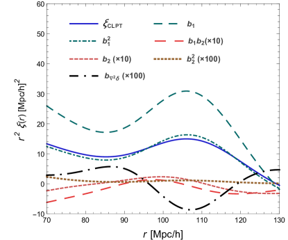
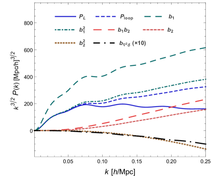
Figure 1: Bias components for the CLPT correlation function [Eq. (II)] and SPT power spectrum [Eq. (22)]. We are also showing the contribution of curvature bias with bias parameter $b_{01}=b_{\nabla^{2}\delta}$ of Sects. III and IV. For the correlation function this is the term that contains $c_{10}c_{01}\nabla^{2}\xi_{R}$ in Eq. (III.1), the second term in that equation is degenerated with this one, while the rest are subdominant. For the power spectrum we are showing $-k^{2}P_{L}(k)$. We fix cosmological parameters to the best fit of the WMAP nine-year results 2013ApJS..208…19H and consider redshift $z=0$.

The SPT power spectrum is obtained by expanding all terms out of the exponential in Eq. (II) and by performing the $q$ integral, obtaining Matsubara:2008wx

$$P^{\text{SPT}}_{X}(k) =P_{L}(k)+P_{22}(k)+P_{13}(k)+b_{1}a_{10}(k)+b_{2}a_{01}(k)+b_{1}^{2}a_{20}(k)+b_{1}b_{2}a_{11}(k)+b_{2}^{2}a_{02}(k),$$ (22)

with

$$P_{22}(k) =\frac{9}{98}Q_{1}(k)+\frac{3}{7}Q_{2}(k)+\frac{1}{2}Q_{3}(k),\qquad P_{13}(k)=\frac{10}{21}R_{1}(k)+\frac{6}{7}R_{2}(k)-\sigma^{2}_{L}k^{2}P_{L}(k),$$ (23)

$$a_{10}(k) =2P_{L}(k)+\frac{10}{21}R_{1}(k)+\frac{6}{7}R_{1+2}(k)+\frac{6}{7}R_{2}(k)+\frac{6}{7}Q_{5}(k)+2(Q_{7}(k)-\sigma^{2}_{L}k^{2}P_{L}(k)),$$ (24)

$$a_{01}(k) =Q_{9}(k)+\frac{3}{7}Q_{8}(k),\qquad a_{20}(k)=P_{L}(k)+\frac{6}{7}R_{1+2}(k)+Q_{9}(k)+Q_{11}(k)-\sigma^{2}_{L}k^{2}P_{L}(k),$$ (25)

$$a_{11}(k) =2Q_{12}(k),\qquad a_{02}(k)=\frac{1}{2}Q_{13}(k),$$ (26)

$$\sigma^{2}_{L} =\frac{1}{3}\delta_{ij}\langle\Psi_{i}(0)\Psi_{j}(0)\rangle=\frac{1}{6\pi^{2}}\int dpP_{L}(p).$$ (27)

In Fig. 1 we show the different contributions to Eq. (22). The $Q(k)$ and $R(k)$ functions are computed for Einstein-de Sitter (EdS) evolution in Matsubara:2007wj ; Matsubara:2008wx , however, they can differ in more general cosmologies Aviles:2017aor . In particular, in $\Lambda$CDM we have that $R_{1}+R_{2}\simeq R_{1+2}$ is a good approximation, holding exactly in EdS. The claim that Eq. (22) contains the standard pieces in the unbiased SPT power spectrum was proven in Matsubara:2007wj for EdS and more generally in Vlah:2014nta .

We notice Eq. (22) is the SPT power spectrum for locally biased tracers at initial time, which we emphasize differs from the power spectrum of Eulerian local biased tracers, because smoothing and nonlinear evolution do not commute. Only at linear order in fluctuations these are simple related since $P_{XL}(k)=(1+b_{1})^{2}P_{L}(k)$, consistent with Eq. (20). However, at large scales the biased power spectrum does not reduce to the linear one, instead we have

$$P_{X}^{\text{SPT}}(k\rightarrow 0)=(1+b_{1})^{2}P_{L}(k)+\frac{1}{2}b_{2}^{2}\int\frac{d^{3}p}{(2\pi)^{3}}(P_{L}(p))^{2}.$$ (28)

The constant term arises from the last term in Eq. (22),

$$a_{02}(k)=\frac{1}{2}\int\frac{d^{3}p}{(2\pi)^{3}}P_{L}(p)P_{L}(|{\text{\bf k}}-{\text{\bf p}}|),$$ (29)

which is potentially harmful. For power law power spectra with $P_{L}\propto k^{n}$, $a_{02}(k)$ is UV divergent for $n\geq-3/2$ (instead of $P_{loop}$, whose UV divergence appears for $n\geq-1$). The filtering makes $a_{02}(k)$ convergent but sensible to the cutoff $\Lambda=1/R_{\Lambda}$. Thus, scales below $\Lambda$ receive arbitrary corrections from the small scales that were integrated out of the theory. Exactly the same constant contribution to the power spectrum is present in the biased SPT power spectrum with already renormalized Eulerian bias, that is cured by considering the addition of a constant shot noise to the biased power spectrum McDonald:2006mx , which at this point we introduce as $P_{X}\rightarrow P_{X}+N_{0}$. This white noise arises from stochastic, uncorrelated with long wavelength overdensities, contributions to the density fields of tracers, and is renormalized to absorb the term $a_{02}(k=0)$. Slightly more formally, in Eq. (7) we may add a contribution $X_{\epsilon}=\lambda_{\epsilon,1}\epsilon_{0}({\text{\bf q}}_{1})+\lambda_{\epsilon,2}\epsilon_{0}({\text{\bf q}}_{2})$ that comes from stochasticity of small scales, inducing the constant $N_{0}=b_{\epsilon}^{2}\langle\epsilon_{0}({\text{\bf k}})\epsilon_{0}({\text{\bf k}}^{\prime})\rangle$ contribution to the power spectrum (see Sec. IV). Thereafter, the bias parameter $b_{\epsilon}$ absorbs the constant $a_{02}(k=0)$, leading to a renormalized function

$$a_{02}(k)\longrightarrow a_{02}(k)-a_{02}(0)=\frac{1}{2}\int\frac{d^{3}p}{(2\pi)^{3}}P_{L}(p)(P_{L}(|{\text{\bf k}}-{\text{\bf p}}|)-P_{L}(p)),$$ (30)

which is safe from UV divergences for $n<-1/2$. By taking the inverse Fourier transform of the renormalized function $a_{02}(k)$, the constant shift only contributes with a Dirac delta function at $r=0$ in the correlation function.

There are other divergences in Eq. (22). $Q_{3}(k)$ has IR divergences when the internal momentum goes to zero and when it approaches the external momentum; both divergences are canceled by the term $2\sigma^{2}_{L}k^{2}P_{L}$ Aviles:2017aor . Functions $Q_{7}(k)$ and $Q_{11}(k)$ present the same IR divergence when the internal momenta go to zero, but we note that they are accompanied by $\sigma^{2}_{L}k^{2}P_{L}$ terms; hence these divergences cancel out, becoming IR safe for spectral index $n>-3$. All the other functions in Eq. (22) are well behaved.

III Curvature bias and renormalization

III.1 Density curvature bias

To some extent, we have removed the $R_{\Lambda}$ dependence from statistics in the sense that they lack zero-lag correlators. However, there still exist some residual dependencies. Consider the linear correlation function of smoothed density fields Schmidt:2012ys

$$\xi_{R}(q)=\int\frac{d^{3}k}{(2\pi)^{3}}e^{i{\text{\bf k}}\cdot{\text{\bf q}}}|\tilde{W}(kR_{\Lambda})|^{2}P_{L}(k)=\xi(q)+2R_{\Lambda}^{2}\nabla^{2}\xi(q)+\mathcal{O}(R_{\Lambda}^{4}\nabla^{4}\xi(q)),$$ (31)

where we expanded the smoothing filter as $\tilde{W}(kR_{\Lambda})=1-R_{\Lambda}^{2}k^{2}+\cdots$ for illustration purposes, though our results do not depend in this particular choice. Equation (31) shows that the linear correlation function will be $R_{\Lambda}$ independent as long as $R^{2}_{\Lambda}\nabla^{2}\xi(r)\ll\xi(r)$. For a featureless correlation function this holds as long as $R_{\Lambda}\ll r$, but in our Universe where the BAO bump with a width $\Delta r\sim 20\,\text{Mpc}/h$ is present at a scale $r\sim 100\,\text{Mpc}/h$, the condition becomes $R_{\Lambda}\ll\Delta r$, which is highly undesirable, especially for the description of massive halos where the smoothing scale is typically identified with its Lagrangian radius. In this section, following closely the work of Ref. Schmidt:2012ys , we remove the subleading scale dependencies by introducing a density Laplacian as an argument in the Lagrangian bias function,

$$1+\delta_{X}=F(\delta_{R},\nabla^{2}\delta_{R}),$$ (32)

which generalizes the LPT power spectrum for tracers,

$$(2\pi)^{3}\delta_{\text{D}}({\text{\bf k}})+P_{X}(k)=\int d^{3}qe^{i{\text{\bf k}}\cdot{\text{\bf q}}}\int\frac{d^{2}\mathbf{\Lambda}_{1}}{(2\pi)^{2}}\frac{d^{2}\mathbf{\Lambda}_{2}}{(2\pi)^{2}}\tilde{F}(\mathbf{\Lambda}_{1})\tilde{F}(\mathbf{\Lambda}_{2})\langle e^{i[\mathbf{\Lambda}_{1}\cdot\mathbf{D}_{1}+\mathbf{\Lambda}_{2}\cdot\mathbf{D}_{2}+{\text{\bf k}}\cdot\Delta]}\rangle,$$ (33)

where

$$\mathbf{\Lambda}=(\lambda,\bar{\eta}),\qquad\mathbf{D}=(\delta_{R},\nabla^{2}\delta_{R})$$ (34)

are vectors and $\tilde{F}(\mathbf{\Lambda})=\tilde{F}(\lambda,\bar{\eta})$ is the Fourier transform of $F(\delta_{R},\nabla^{2}\delta_{R})$ with respect to both arguments. In the same way that $\lambda$ is the spectral bias parameter of matter overdensities, $\bar{\eta}$ is the (bare) spectral bias parameter for the curvature operator $\nabla^{2}\delta_{R}$. We introduce the bivariate bias parameters as a generalization of Eq. (11):

$$c_{nm}\equiv\int\frac{d^{2}\mathbf{\Lambda}}{(2\pi)^{2}}\tilde{F}(\mathbf{\Lambda})e^{-\frac{1}{2}\mathbf{\Lambda}^{\text{T}}\mathbf{\Sigma}\mathbf{\Lambda}}(i\lambda)^{n}(i\bar{\eta})^{m}=\int\frac{d^{2}\mathbf{D}}{2\pi|\mathbf{\Sigma}|^{1/2}}e^{-\frac{1}{2}\mathbf{D}^{\text{T}}\mathbf{\Sigma}^{-1}\mathbf{D}}\frac{\partial^{n+m}F(\delta_{R},\nabla^{2}\delta_{R})}{\partial\delta^{n}\partial(\nabla^{2}\delta)^{m}}=\left\langle\frac{\partial^{n+m}F(\delta_{R},\nabla^{2}\delta_{R})}{\partial\delta^{n}\partial(\nabla^{2}\delta)^{m}}\right\rangle.$$ (35)

The components of the covariance matrix are given by zero-lag correlators as $\Sigma_{11}=\langle\delta_{R}^{2}\rangle=\sigma^{2}_{R}$, $\Sigma_{12}=\Sigma_{21}=\langle\delta_{R}\nabla^{2}\delta_{R}\rangle$, and $\Sigma_{22}=\langle(\nabla^{2}\delta_{R})^{2}\rangle$. Standard notation is recovered by identifying

$$b_{n}=c_{n0},\qquad\text{and}\qquad c_{(\nabla^{2}\delta)^{m}}=c_{0m}.$$ (36)

We see below that parameters $c_{nm}$ require renormalization, unlike the $b_{n}$ of the previous section. For initial density fields, we get the correlation function for tracers

$$\xi_{X}({\text{\bf q}})=c_{10}^{2}\xi_{R}({\text{\bf q}})+2c_{10}c_{01}\nabla^{2}\xi_{R}({\text{\bf q}})+c_{01}^{2}\nabla^{4}\xi_{R}({\text{\bf q}}),$$ (37)

which extends Eq. (16) by including curvature bias, but simplifies it by considering only linear fluctuations. It is good to keep in mind that $c_{nm}$ has units of $[\text{\emph{length}}]^{2m}$, reflecting the nonlocality of the bias description.

In this subsection, we are interested in removing the $R_{\Lambda}$ dependencies of the $\xi_{R}$ and $\xi_{R}^{2}$ terms of Eq. (II). This can be achieved by considering the following contributions to the LPT power spectrum

$$(2\pi)^{3}\delta_{\text{D}}({\text{\bf k}})+P_{X}^{\text{LPT}}(k) \supset\int d^{3}qe^{i{\text{\bf k}}\cdot{\text{\bf q}}}e^{-\frac{1}{2}k_{i}k_{j}A_{ij}-\frac{i}{6}k_{i}k_{j}k_{k}W_{ijk}}\Big{(}2c_{10}c_{01}\nabla^{2}\xi_{R}(q)-2ic_{01}k_{i}\nabla_{i}\xi_{R}(q)$$

$$\quad+2i(c_{20}c_{01}+c_{10}c_{11})\nabla^{2}\xi_{R}k_{i}U_{i}+2c_{20}c_{11}\xi_{R}\nabla^{2}\xi_{R}\Big{)},$$ (38)

with

$$\nabla^{2}\xi_{R}(q)=-\int\frac{d^{3}k}{(2\pi)^{3}}e^{i{\text{\bf k}}\cdot{\text{\bf q}}}k^{2}|\tilde{W}(kR)|^{2}P_{L}(k)=\nabla^{2}\xi(q)+2R_{\Lambda}^{2}\nabla^{4}\xi(q)+\cdots,$$ (39)

where we expanded the filter $W$ in powers of $R_{\Lambda}^{2}k^{2}$. By expanding loop contributions out of the exponential in Eq. (III.1) and performing the Fourier transform, we arrive at

$$\xi_{X}^{\text{CLPT}}(r) \supset\int\frac{d^{3}q}{(2\pi)^{3/2}|A_{L}|^{1/2}}e^{-\frac{1}{2}(A_{L}^{-1})_{ij}(q_{i}-r_{i})(q_{j}-r_{j})}\Big{(}2c_{10}c_{01}\nabla^{2}\xi_{R}(q)+2c_{01}\nabla_{i}\xi_{R}(q)g_{i}$$

$$\quad-2(c_{20}c_{01}+c_{10}c_{11})\nabla^{2}\xi_{R}g_{i}U_{i}+2c_{20}c_{11}\xi_{R}\nabla^{2}\xi_{R}+\cdots\Big{)}.$$ (40)

A similar result is presented in Vlah:2016bcl , where the authors additionally consider tidal bias and EFT contributions; the latter are degenerated with the curvature bias. By comparing Eqs. (37) and (III.1) we note an interesting fact: once nonlinear evolution takes place, bivariate bias parameters $c_{nm}$, with both $n\neq 0$ and $m\neq 0$, should be considered, and the description with only univariate biases $c_{n0}$ and $c_{0m}$ becomes incomplete. Clearly, this feature is shared by the SPT power spectrum, but we postpone its discussion to Sec. IV.

Joining this result with the $\xi_{R}$ in Eq. (II) and using Eq. (31), the combination

$$c_{10}^{2}(\xi(q)+2R_{\Lambda}^{2}\nabla^{2}\xi(q))+2c_{10}c_{01}\nabla^{2}\xi(q)=c_{10}^{2}\xi(q)+2c_{10}(c_{10}R_{\Lambda}^{2}+c_{01})\nabla^{2}\xi(q)$$ (41)

appears in the correlation function. That is, the curvature bias operator has introduced the precise term in order to absorb the $R_{\Lambda}^{2}$ term in the above equation, since we can reparametrize $b_{01}=c_{01}+c_{10}R_{\Lambda}^{2}$. In this sense, the addition of a curvature bias is not a choice, it should be included to make the theory independent of (or less sensible to) the details of the smoothing.

Another contribution to Eq. (II) sensible to $R_{\Lambda}$ is $\xi_{R}g_{i}U_{i}$. We can pair it with the term $\nabla^{2}\xi_{R}g_{i}U_{i}$ in Eq. (III.1), leading to

$$\left[2c_{10}c_{20}(\xi+2R_{\Lambda}^{2}\nabla^{2}\xi)+2(c_{20}c_{01}+c_{10}c_{11})\nabla^{2}\xi\right]g_{i}U_{i}=\left[2c_{10}c_{20}\xi+2c_{20}(2c_{10}R_{\Lambda}^{2}+c_{01}+\frac{c_{11}c_{10}}{c_{20}})\nabla^{2}\xi\right]g_{i}U_{i}.$$ (42)

One of the terms $c_{10}R^{2}$ is absorbed by $c_{01}$ as in Eq.(41), while the other is absorbed by $\frac{c_{11}c_{10}}{c_{20}}$. That is, we can reparametrize $b_{11}=c_{11}+c_{20}R_{\Lambda}^{2}$.

Analogously, the contribution $\frac{1}{2}c_{20}^{2}\xi^{2}_{R}$ to Eq. (II) is expanded as

$$\frac{1}{2}c_{20}^{2}\xi^{2}_{R}=\frac{1}{2}c_{20}^{2}\xi^{2}+2c_{20}^{2}\xi R_{\Lambda}^{2}\nabla^{2}\xi+\mathcal{O}(R_{\Lambda}^{4}\nabla^{4}\xi).$$ (43)

We join up the second term in the rhs of the above equation with the term $2c_{20}c_{11}\xi_{R}\nabla^{2}\xi_{R}$ in Eq. (III.1), the sum of both is

$$2\frac{c^{2}_{20}}{c_{10}}\left(c_{10}R_{\Lambda}^{2}+\frac{c_{11}c_{10}}{c_{20}}\right)\xi\nabla^{2}\xi+\cdots,$$ (44)

and consistently with Eq. (42), the term $\frac{c_{11}c_{10}}{c_{20}}$ absorbs $c_{10}R_{\Lambda}^{2}$.

III.2 Renormalization of curvature and higher order bias via spectral parameters

The renormalization presented in the previous subsection is a special case of a more general method that is the subject of this subsection. We can guarantee that our results are $R_{\Lambda}$ independent if we are able to remove any $R_{\Lambda}$ dependence in the function $X$ [Eq. (7)]. We focus on just one term, $X_{\delta}=\lambda\delta_{R}$, and use

$$\delta_{R}({\text{\bf q}})=\int\frac{d^{3}k}{(2\pi)^{3}}e^{i{\text{\bf k}}\cdot{\text{\bf q}}}\tilde{W}(kR_{\Lambda})\delta({\text{\bf k}})=\sum_{n=0}^{\infty}(-1)^{n}W_{n}R_{\Lambda}^{2n}\nabla^{2n}\delta({\text{\bf q}})$$ (45)

where we assumed that the filter can be Taylor expanded as $\tilde{W}(kR)=\sum_{n=0}^{\infty}W_{n}(kR_{\Lambda})^{2n}$; we notice that normalization of the window function, $\int d^{3}xW({\text{\bf x}})=1$, implies $W_{0}=1$. To absorb the smoothing scale we add a (formally infinite) collection of counterterms

$$Y=\sum_{m=1}^{\infty}\bar{\eta}_{\nabla^{2m}\delta}\nabla^{2m}\delta_{R}({\text{\bf q}}).$$ (46)

where $\bar{\eta}_{\nabla^{2m}\delta}$ is a set of unrenormalized spectral parameters; in the notation of the previous subsection $\bar{\eta}=\bar{\eta}_{\nabla^{2}\delta}$. Inserting Eq. (45) in Eq. (46) and summing to $X_{\delta}$ we get

$$X_{\delta}+Y =\lambda\delta({\text{\bf q}})+\sum_{n=1}^{\infty}\left((-1)^{n}\lambda W_{n}R_{\Lambda}^{2n}+\sum_{m=1}^{n}(-1)^{n-m}W_{n-m}R_{\Lambda}^{2(n-m)}\bar{\eta}_{\nabla^{2m}\delta}\right)\nabla^{2n}\delta({\text{\bf q}})$$ (47)

where we used the double sum identity $\sum_{m=1}^{\infty}\sum_{n=0}^{\infty}=\sum_{i=1}^{\infty}\sum_{m=1}^{i}$ with $i=m+n$, and relabel $i\rightarrow n$.

We introduce the renormalized bias spectral parameters as

$$\eta_{\nabla^{2n}\delta}=(-1)^{n}W_{n}R_{\Lambda}^{2n}\left(\lambda+\sum_{m=1}^{n}(-1)^{m}\frac{W_{n-m}}{W_{n}R_{\Lambda}^{2m}}\bar{\eta}_{\nabla^{2m}\delta}\right),$$ (48)

from which

$$X_{\delta}+Y =\lambda\delta({\text{\bf q}})+\sum_{n=1}^{\infty}\eta_{\nabla^{2n}\delta}\nabla^{2n}\delta({\text{\bf q}}),$$ (49)

becomes $R_{\Lambda}$ independent.

We have introduced an infinite set of counterterms; in this case zero-lag correlators in the covariance matrix $\mathbf{\Sigma}$ diverge for common linear power spectra. In practice, only a finite set of counterterms can be introduced, let us say up to $n=N$, keeping dependencies $\sim\mathcal{O}(R_{\Lambda}^{2(N+1)}\nabla^{2(N+1)}\delta_{R})$, and as one approaches the smoothing scale, the theory loses its validity.

We now come back to the case in which only the counterterm $\nabla^{2}\delta_{R}$ is introduced. From Eq. (48), the spectral renormalized parameter $\eta=\eta_{\nabla^{2}\delta}$ is

$$\eta=\bar{\eta}-W_{1}R_{\Lambda}^{2}\lambda.$$ (50)

We define the bivariate renormalized bias parameters as

$$b_{nm}\equiv\int\frac{d\mathbf{\Lambda}}{(2\pi)^{2}}e^{-\frac{1}{2}\mathbf{\Lambda}^{T}\mathbf{\Sigma}\mathbf{\Lambda}}\tilde{F}(\mathbf{\Lambda})(i\lambda)^{n}(i\eta)^{m},$$ (51)

where we note that we still have $\mathbf{\Lambda}=(\lambda,\bar{\eta})$. Replacing $\bar{\eta}$ for $\eta$, we get

$$b_{nm}=\sum_{k=0}^{m}\binom{m}{k}(-W_{1})^{k}R_{\Lambda}^{2k}c_{n+k,m-k},$$ (52)

which relates renormalized and unrenormalized bivariate biases. We immediately have $b_{n0}=c_{n0}$ and

$$b_{01}=c_{01}-W_{1}R_{\Lambda}^{2}c_{10},\qquad b_{11}=c_{11}-W_{1}R_{\Lambda}^{2}c_{20}.$$ (53)

By setting $W_{1}=-1$, as in the previous subsection, we note that these are the precise relations we need to make the $R_{\Lambda}$ cancellations in Eqs. (41), (42) and (44).

We can extend the definitions of bivariate bias in Eqs.(35) and (51) to include higher-derivative terms. That is, we introduce the bare and renormalized multivariate bias parameters as

$$c_{n_{0}n_{1}\cdots n_{N}}=\int\frac{d\mathbf{\Lambda}}{(2\pi)^{N+1}}e^{-\frac{1}{2}\mathbf{\Lambda}^{\text{T}}\mathbf{\Sigma}\mathbf{\Lambda}}\tilde{F}(\mathbf{\Lambda})(i\lambda)^{n_{0}}(i\bar{\eta}_{\nabla^{2}\delta})^{n_{1}}\cdots(i\bar{\eta}_{\nabla^{2N}\delta})^{n_{N}},$$ (54)

$$b_{n_{0}n_{1}\cdots n_{N}}=\int\frac{d\mathbf{\Lambda}}{(2\pi)^{N+1}}e^{-\frac{1}{2}\mathbf{\Lambda}^{\text{T}}\mathbf{\Sigma}\mathbf{\Lambda}}\tilde{F}(\mathbf{\Lambda})(i\lambda)^{n_{0}}(i\eta_{\nabla^{2}\delta})^{n_{1}}\cdots(i\eta_{\nabla^{2N}\delta})^{n_{N}},$$ (55)

with $\mathbf{\Lambda}=(\lambda,\bar{\eta}_{\nabla^{2}\delta},\dots,\bar{\eta}_{\nabla^{2N}\delta})$ and $\Sigma_{ij}=\langle\nabla^{2(i-1)}\delta_{R}\nabla^{2(j-1)}\delta_{R}\rangle$. Analogous relations to Eq. (52) follow from substituting Eq. (48) in Eq. (55). To check consistency with earlier work, we consider the case

$$b_{\nabla^{2N}\delta}\equiv b_{\underbrace{\scriptstyle{00\cdots 1}}_{N+1}}.$$ (56)

Using the spectral bias parameters relation of Eq. (48), we quickly find the relation between renormalized and bare bias parameters:

$$b_{\nabla^{2N}\delta}=\sum_{m=0}^{N}(-1)^{N-m}W_{N-m}R_{\Lambda}^{2(N-m)}c_{\nabla^{2m}\delta},$$ (57)

which is the same result presented in Eq. (B14) of Ref. Schmidt:2012ys , with $[W_{n}]^{\text{here}}=[\frac{(-1)^{n}f_{n}}{(2n+1)!}]^{\text{that work}}$.

The connection between our formalism and the peak background split bias (PBS) framework Mo:1996cn ; Schmidt:2012ys is deeper than the above result. In the PBS formalism the bias parameters are defined as responses of the mean abundance of tracers to small changes of background density and curvature. If the background density $\bar{\rho}$ is shifted by a constant amount $\Delta\bar{\rho}=\bar{\rho}D$, the smoothed overdensity is shifted as

$$\bar{\rho}\rightarrow\bar{\rho}+\bar{\rho}D:\qquad\delta_{R}\rightarrow\delta_{R}+D.$$ (58)

On the other hand, a constant shift on the curvature $\nabla^{2}\delta\rightarrow\nabla^{2}\delta+\alpha$ induces a shift on the Laplacian of the smoothed density and on the smoothed density itself

$$\nabla^{2}\delta\rightarrow\nabla^{2}\delta+\alpha:\qquad\nabla^{2}\delta_{R}\rightarrow\nabla^{2}\delta_{R}+\alpha,\quad\delta_{R}\rightarrow\delta_{R}-W_{1}R_{\Lambda}^{2}\alpha,$$ (59)

where the last relation holds if the density field $\delta$ is evaluated at the center of the window function (see Schmidt:2012ys ), otherwise subdominant terms should be added. For bivariate bias parameters we simply take the combined transformation, $\delta_{R}\rightarrow\delta_{R}+D-W_{1}R_{\Lambda}^{2}\alpha$, $\nabla^{2}\delta\rightarrow\nabla^{2}\delta+\alpha$. Since in this work we have defined $F$ through Eq. (32), the mean abundance of tracers $n_{X}$ at position x is given by $n_{X}({\text{\bf x}})=\langle n_{X}\rangle_{{\text{\bf x}}}F$, and the PBS biases are

$$b_{nm}^{\text{PBS}}=\left\langle\frac{\partial^{n+m}F(\delta+D-W_{1}R_{\Lambda}^{2}\alpha,\nabla^{2}\delta+\alpha)}{\partial D^{n}\partial\alpha^{m}}\Big{|}_{\alpha=0,D=0}\right\rangle.$$ (60)

We want to show that this coincides with our definition of bias in Eq. (51). First, we have

$$F(\delta+D-W_{1}R_{\Lambda}^{2}\alpha,\nabla^{2}\delta+\alpha)=\int\frac{d\Lambda}{2\pi}\frac{d\eta}{2\pi}e^{i\lambda\delta+i\bar{\eta}\nabla^{2}\delta}F(\lambda,\bar{\eta})e^{iD\lambda+i\alpha(\bar{\eta}-W_{1}\lambda R_{\Lambda}^{2})}.$$ (61)

By taking derivatives with respect to $D$ and $\alpha$,

$$\frac{\partial^{n+m}F(\delta+D-W_{1}R_{\Lambda}^{2}\alpha,\nabla^{2}\delta+\alpha)}{\partial D^{n}\partial\alpha^{m}}\Big{|}_{\alpha=0,D=0} =\int\frac{d\Lambda}{2\pi}\frac{d\eta}{2\pi}e^{i\lambda\delta+i\bar{\eta}\nabla^{2}\delta}F(\lambda,\bar{\eta})(i\lambda)^{n}(i\bar{\eta}-iW_{1}R_{\Lambda}^{2})^{m}$$

$$=\int\frac{d\mathbf{\Lambda}}{(2\pi)^{2}}e^{i\mathbf{\Lambda}\cdot\mathbf{D}}F(\mathbf{\Lambda})(i\lambda)^{n}(i\eta)^{m},$$ (62)

where in the last equality we have used $\eta=\bar{\eta}-W_{1}R_{\Lambda}^{2}$, consistently with Eq. (50). Now, we assume ergodicity and Gaussianity to obtain the PBS biases, that is, integration of Eq. (III.2) against $\int d\mathbf{D}(2\pi|\mathbf{\Sigma}|^{1/2})^{-1}e^{-\frac{1}{2}\mathbf{D}^{T}\mathbf{\Sigma}^{-1}\mathbf{D}}$ yields

$$b_{nm}^{\text{PBS}} =\int\frac{d\mathbf{\Lambda}}{(2\pi)^{2}}e^{-\frac{1}{2}\mathbf{\Lambda}^{T}\mathbf{\Sigma}\mathbf{\Lambda}}\tilde{F}(\mathbf{\Lambda})(i\lambda)^{n}(i\eta)^{m}=b_{nm},$$ (63)

which shows the equivalence of our renormalized bias with the PBS biases.

We emphasize that our results rely on the reparametrization of spectral bias parameters of Eq. (48). Any multivariate renormalized bias parameter is found through Eq. (55), and to find the relation between the $c_{n_{1}n_{2}\dots}$ and $b_{n_{1}n_{2}\dots}$ one uses Eq. (48) and performs combinatorial algebra.

IV Renormalization of contact terms

The SPT power spectrum corresponding to Eq. (III.1) is

$$P^{\text{SPT}}_{X}(k) \ni-2(1+b_{10})b_{01}k^{2}P_{L}(k)-2(b_{20}b_{01}+b_{10}b_{11})\int\frac{d^{3}p}{(2\pi)^{3}}\frac{({\text{\bf k}}-{\text{\bf p}})^{2}{\text{\bf k}}\cdot{\text{\bf p}}}{p^{2}}P_{L}(|{\text{\bf k}}-{\text{\bf p}}|)P_{L}(p)$$

$$\quad-2b_{20}b_{11}\int\frac{d^{3}p}{(2\pi)^{3}}p^{2}P_{L}(|{\text{\bf k}}-{\text{\bf p}}|)P_{L}(p).$$ (64)

The last contribution, named here as $\bar{\mathcal{I}}^{(0,2)}(k)$, is analogous to the function $a_{02}(k)$ that we found in Sec. II. But, this time the UV divergence cannot be removed by a white noise absorbing a constant $\bar{\mathcal{I}}^{(0,2)}(k=0)=\int_{\text{\bf p}}p^{2}P_{L}^{2}(p)$. It is clear that the situation will still get worse as higher derivatives are considered. For example, in Eq. (A) we find the term $b_{02}^{2}(\nabla^{4}\xi)^{2}$, leading to a SPT power spectrum contribution $\int_{|{\text{\bf p}}|<\Lambda}({\text{\bf k}}-{\text{\bf p}})^{4}p^{4}P_{L}(|{\text{\bf k}}-{\text{\bf p}}|)P_{L}(p)$, which scales as $\Lambda^{10+2n}$, with $n$ the spectral index of the linear power spectrum at small scales. The same divergences are present in the Eulerian treatment of bias Assassi:2014fva , and it is well known that these can be absorbed by the stochastic bias. The subject of this section is to provide a systematic procedure to remove these divergences.

Stochastic fields are, by construction, uncorrelated with long wavelength perturbations and among themselves at scales beyond $r>1/\Lambda$ Dekel:1998eq . In principle, they contain all the nonlinear processes that we have smoothed, as much as in the EFTofLSS Baumann:2010tm . In Fourier space its 2-point function is commonly written as 2009JCAP…08..020M ; Desjacques:2016bnm

$$\langle\epsilon({\text{\bf k}})\epsilon({\text{\bf k}}^{\prime})\rangle^{\prime}=N_{0}+N_{1}k^{2}+N_{2}k^{4}+\cdots.$$ (65)

The departure of a white noise arises because stochasticity is not localized at a single point; instead it is a nonlocal process with a range of coherence $\sim 1/\Lambda$, and for the same reason the above description breaks down for $k\sim\Lambda$. The absence of odd powers of $k$ comes from the spherical symmetry of the filter.

The last term in Eq. (IV) is the Fourier transform of one of the many products of correlators evaluated at the same point (commonly named contact terms) we find in the correlation function. In full generality, we find integrals as

$$\bar{\mathcal{I}}^{(s,t)}(k,\Lambda)\equiv(-1)^{t+s}\mathcal{F}[(\nabla^{2s}\xi({\text{\bf q}}))(\nabla^{2t}\xi({\text{\bf q}}))]=\int\frac{d^{3}p}{(2\pi)^{3}}|{\text{\bf k}}-{\text{\bf p}}|^{2t}p^{2s}P_{L}(|{\text{\bf k}}-{\text{\bf p}}|)P_{L}(p),$$ (66)

where we have written explicitly the cutoff dependence. For a scale invariant power spectrum, $P_{L}\propto p^{n}$, $\bar{\mathcal{I}}^{(s,t)}$ scales as $\Lambda^{2(n+s+t+1)}$. Our goal is to find a renormalized function $\mathcal{I}^{(s,t)}$ with two properties: first, that it is UV safe (for $n<-1/2$, for example), and second, that it can be written as the sum of the bare function (Eq. (66)) and a finite set of counterterms:

$$\mathcal{I}^{(s,t)}(k)=\bar{\mathcal{I}}^{(s,t)}(k,\Lambda)+\mathcal{I}^{(s,t)}_{ct}(k,\Lambda),$$ (67)

with counterterms

$$\mathcal{I}^{(s,t)}_{ct}(k,\Lambda)=\mathcal{I}_{0}(\Lambda)+\mathcal{I}_{1}(\Lambda)k^{2}+\cdots+\mathcal{I}_{m}(\Lambda)k^{2m},$$ (68)

for some integer $m$ and with $\mathcal{I}_{i}(\Lambda)$ depending only on the cutoff $\Lambda$. In such a way, the counterterms can be absorbed by stochastic bias terms. We first write the expansion

$$|{\text{\bf k}}-{\text{\bf p}}|^{2t}P_{L}(|{\text{\bf k}}-{\text{\bf p}}|)=p^{2t}P_{L}(p)\sum_{\ell=0}^{\infty}c_{\ell}(\mu^{\ell},\mu^{\ell-2},\dots)\frac{k^{\ell}}{p^{\ell}},$$ (69)

where we have assumed $p^{s}P^{(s)}_{L}(p)\propto P_{L}(p)$, which is a good approximation for large $p$ and holds exactly for scale invariant universes. The $c_{\ell}$ are polynomials of $\mu=\hat{{\text{\bf k}}}\cdot\hat{{\text{\bf p}}}$ with $c_{0}=1$ and containing only even (odd) powers of $\mu$ if $\ell$ is even (odd). We propose the counterterms

$$\mathcal{I}_{ct}^{(s,t)}({\text{\bf k}},\Lambda)=-\int\frac{d^{3}p}{(2\pi)^{3}}p^{2(s+t)}(P_{L}(p))^{2}\sum_{\ell=0}^{2(s+t)}c_{\ell}(\mu^{\ell},\mu^{\ell-2},\dots)\frac{k^{\ell}}{p^{\ell}}.$$ (70)

Thus our candidate for renormalized $\mathcal{I}$ is

$$\mathcal{I}^{(s,t)}(k) =\int\frac{d^{3}p}{(2\pi)^{3}}p^{2s}P_{L}(p)\left(|{\text{\bf k}}-{\text{\bf p}}|^{2t}P_{L}(|{\text{\bf k}}-{\text{\bf p}}|)-p^{2t}P_{L}(p)\sum_{\ell=0}^{2(s+t)}c_{\ell}(\mu^{\ell},\mu^{\ell-2},\dots)\frac{k^{\ell}}{p^{\ell}}\right).$$ (71)

By plugging in the expansion (69) into the above equation we get

$$\mathcal{I}^{(s,t)}(k) =\sum_{\ell=2(s+t)+1}^{\infty}k^{\ell}\int\frac{d^{3}p}{(2\pi)^{3}}c_{\ell}(\mu^{\ell},\mu^{\ell-2},\dots)p^{2(s+t)-\ell}(P_{L}(p))^{2}=\alpha k^{2(s+t)+2}\int\frac{d^{3}p}{(2\pi)^{3}}\frac{(P_{L}(p))^{2}}{p^{2}}+\cdots,$$ (72)

where the first term in the sum of the first equality vanishes when performing the angular integral because $c_{2(s+t)+1}$ is odd in $\mu$. The last equality shows that the renormalized function $\mathcal{I}$ is UV safe for spectral index $n<-1/2$ (the rest of the terms, not shown, are even more convergent; here $\alpha=2\int_{-1}^{1}d\mu\,c_{2(s+t)+2}$ is a number. To complete the proof that $\mathcal{I}^{(s,t)}$ is indeed the renormalized function we are searching for, we need to show that the counterterms can be written in the form of Eq. (67). This follows immediately from Eq. (70) because contributions with $\ell$ odd vanish, and we can write

$$\mathcal{I}_{ct}^{(s,t)}(k,\Lambda)=-\sum_{i=0}^{s+t}\alpha_{i}k^{2i}\int\frac{d^{3}p}{(2\pi)^{3}}p^{2(s+t-i)}(P_{L}(p))^{2}.$$ (73)

At this point one may wonder if this procedure can be continued indefinitely by cutting the sum in Eq. (70) at some $N>2(s+t)$ and making the renormalized function $\mathcal{I}$ as close to zero as desired. While this is true, it would require an arbitrary number of stochastic bias operators, as we see below.

We can accommodate the stochastic fields in the approach we have followed by adding $\epsilon({\text{\bf q}})$ as a new argument to the Lagrangian bias function $F$, which introduces a spectral bias $\lambda_{\epsilon}$ and corresponding bias parameters $b_{\epsilon},b_{\epsilon^{2}},\dots$. Thereafter we expand similarly to Eq. (45), $\epsilon({\text{\bf q}})\simeq\epsilon_{0}({\text{\bf q}})+\alpha R_{\Lambda}^{2}\nabla^{2}\epsilon_{0}({\text{\bf q}})+\cdots$, with $\alpha$ a number whose value is not important for our discussion. This suggests introducing a second stochastic bias operator $\nabla^{2}\epsilon$ with its own bias spectral parameter $\eta_{\nabla^{2}\epsilon}$ and a set of bias parameters $\{b_{(\nabla^{2}\epsilon)^{N}}\}$. Since the stochastic terms are uncorrelated with long wavelength overdensities and among themselves at large scales, we have $\langle\epsilon({\text{\bf q}}_{1})\epsilon({\text{\bf q}}_{2})\rangle_{|{\text{\bf q}}|>R_{\Lambda}}=0$ and $\langle\epsilon({\text{\bf q}}_{1})\delta_{R}({\text{\bf q}}_{2})\rangle=0$, and equivalent equations for $\nabla^{2}\epsilon$. Accordingly, the covariance matrix $\mathbf{\Sigma}$ will have an isolated block including only zero-lag correlators of stochastic fields, and connected correlators of stochastic fields will be singled out in tracer statistics. Up to second order in stochastic bias expansion we found terms up to $(b_{(\nabla^{2}\epsilon)^{2}}\langle\nabla^{2}\epsilon\nabla^{2}\epsilon\rangle)^{2}$, more precisely, we get the SPT power spectrum for stochastic fields

$$P_{\epsilon}({\text{\bf k}}) =\int d^{3}qe^{-i{\text{\bf k}}\cdot{\text{\bf q}}}\Big{(}b^{2}_{\epsilon}\xi_{\epsilon}+b_{\epsilon}b_{\nabla^{2}\epsilon}\nabla^{2}\xi_{\epsilon}+b_{\nabla^{2}\epsilon}^{2}\nabla^{4}\xi_{\epsilon}+\frac{1}{2}b^{2}_{\epsilon^{2}}\xi_{\epsilon}^{2}+(b_{\epsilon^{2}}b_{(\nabla^{2}\epsilon)^{2}}+b_{\epsilon}^{2}b_{\nabla^{2}\epsilon}^{2})(\nabla^{2}\xi_{\epsilon})^{2}+\frac{1}{2}b^{2}_{(\nabla^{2}\epsilon)^{2}}(\nabla^{4}\xi_{\epsilon})^{2}$$

$$\quad\qquad+2b_{\epsilon}^{2}b_{\epsilon,\nabla^{2}\epsilon}\xi_{\epsilon}\nabla^{2}\xi_{\epsilon}+b_{\epsilon,\nabla^{2}\epsilon}^{2}\xi_{\epsilon}\nabla^{4}\xi_{\epsilon}+b_{\epsilon,\nabla^{2}\epsilon}b_{(\nabla^{2}\epsilon)^{2}}\nabla^{2}\xi_{\epsilon}\nabla^{4}\xi_{\epsilon})$$

$$=(a_{0}+a_{1}k^{2}+a_{2}k^{4})\mathcal{F}[\xi_{\epsilon}]+(b_{0}+b_{1}k^{2}+b_{2}k^{4}+b_{3}k^{6}+b_{4}k^{8})\mathcal{F}[\xi_{\epsilon}^{2}]$$ (74)

with

$$\xi_{\epsilon}(q)\equiv\langle\epsilon_{0}({\text{\bf q}}_{1})\epsilon_{0}({\text{\bf q}}_{1}+{\text{\bf q}})\rangle,$$ (75)

and $a_{0},\dots,b_{4}$ combinations of the stochastic bias parameters. Since $\xi_{\epsilon}(q)$ vanishes quickly for $q>R_{\Lambda}$, we expect that $\mathcal{F}[\xi_{\epsilon}]$ and $\mathcal{F}[\xi_{\epsilon}^{2}]$ depend weakly on $k$ for $k\ll\Lambda$, being effectively constants at large scales. It is common to assign $\xi_{\epsilon}(q)=P^{\{0\}}_{\epsilon}\delta_{\text{D}}({\text{\bf q}})$ Desjacques:2016bnm , leading to $\mathcal{F}[\xi_{\epsilon}]=P^{\{0\}}_{\epsilon}$, but ill defined for $\mathcal{F}[\xi_{\epsilon}^{2}]$.

The derivation of Eq. (IV) was informal because our model for stochasticity is far from being rigorous. Hence it should be considered as indicative, almost illustrative; c.f. Sec. 2.8 of Desjacques:2016bnm . However, our objective was to make notice that with the introduction of two stochastic bias operators $\epsilon$ and $\nabla^{2}\epsilon$ and with a second order bias expansion, we obtain powers up to $k^{8}$ in Eq. (IV). This is the equivalent to Eq. (A) where we consider bias operators $\delta$ and $\nabla^{2}\delta$ and we have contact terms up to $b_{02}^{2}(\nabla^{4}\xi)^{2}$, which has $s+t=4$, and Eq. (73) contains powers up to $k^{8}$ also. Therefore, to remove the UV divergences of contact terms we consider a Lagrangian bias function $F(\delta,\nabla^{2}\delta,\epsilon,\nabla^{2}\epsilon)$. If we add an argument $\nabla^{4}\delta$, in order to preserve the same level of convergence we should add $\nabla^{4}\epsilon$ as well.

V Conclusions

In this work we proposed a novel method of renormalization of Lagrangian bias, consisting of a reparametrization of a set of spectral parameters, which we define as the arguments of the Fourier transformed Lagrangian bias function $\tilde{F}(\lambda,\eta_{\nabla^{2}\delta},\cdots)$. From this renormalized spectra one can easily find any multivariate bias parameter as a function of the bare biases. Our definition for nonlocal bias is an extension of the local case introduced by Matsubara Matsubara:2008wx in order to include curvature and higher-derivative operators. We noticed that the local biases were already renormalized in the sense that 2-points statistics of biased tracers contain only connected moments. However, we find the necessity of add curvature bias to remove subleading dependencies on the smoothing scale. We have restricted our discussion to Gaussian fields and 2-point functions nonlinearly evolved by PT, but it would be attractive to generalize our results to $N$-point statistics and non-Gaussian initial conditions.

We checked the consistency of our results by comparing to the PBS biases of Schmidt:2012ys . In fact, our multivariate bias parameters are shown to be equivalently obtained from the PBS argument in the case of initial Gaussian fields. We believe that our renormalization is simpler than previous methods because it only relies on one relation between bare and bias spectral parameters—Eq. (48), which is a key result of this work.

We further developed a systematic procedure to remove UV divergences of Fourier transformed contact terms. Although it was known from previous works that this is doable due to stochasticity, to our knowledge this is the first time that an explicit method to do it is presented. Our model for stochasticity is primitive, but we find it well motivated, and indeed it provides the necessary contributions to the power spectrum in order to absorb the UV divergences coming from contact terms.

An obvious extension of this work is to additionally consider nonlinear biases such as tidal bias. We do not foresee major complications for doing so following the same path of Ref.Vlah:2016bcl . Another interesting direction is to pursue similar methods to the case of Eulerian bias renormalization; such an endeavor would require the introduction of all bias operators consistent with the symmetries of the fluid equations up to the desired order in PT, including operators that cannot be expressed in terms of matter overdensities Assassi:2014fva .

Finally, we note that similar renormalization schemes (such as that of contact terms) are required in the EFTofLSS; hence we believe the methods developed here can find applicability in that theory.

Appendix A 2nd order in curvature and local bias expansion

In this appendix we provide an equation for the LPT power spectrum with local and curvature bias up to second order in bias expansion. We replace Eq. (7) by

$$X=\lambda_{1}\delta_{1}+\lambda_{2}\delta_{2}+\eta_{1}\nabla^{2}\delta_{1}+\eta_{2}\nabla^{2}\delta_{2}+{\text{\bf k}}\cdot\Delta$$ (76)

and define

$$\sigma^{2}_{R}=\langle(\delta_{R})^{2}\rangle_{c},\qquad\sigma^{2}_{\delta\nabla^{2}\delta} =\langle\delta_{R}\nabla^{2}\delta_{R}\rangle_{c},\qquad\sigma^{2}_{\nabla^{2}\delta}=\langle(\nabla^{2}\delta_{R})^{2}\rangle_{c}.$$ (77)

With this, we get

$$-\frac{1}{2}\langle X^{2}\rangle_{c} =-\frac{1}{2}(\lambda_{1}^{2}+\lambda_{2}^{2})\sigma^{2}_{R}-\frac{1}{2}(\eta_{1}^{2}+\eta_{2}^{2})\sigma^{2}_{\nabla^{2}\delta}-(\lambda_{1}\eta_{1}+\lambda_{2}\eta_{2})\sigma^{2}_{\delta\nabla^{2}\delta}-\lambda_{1}\lambda_{2}\xi_{R}-(\lambda_{1}+\lambda_{2})k_{i}U_{i}-\frac{1}{2}k_{i}k_{j}A_{ij}$$

$$\quad-(\lambda_{1}\eta_{2}+\lambda_{2}\eta_{1})\nabla^{2}\xi_{R}+(\eta_{1}+\eta_{2})k_{i}\nabla_{i}\xi_{R}+\eta_{1}\eta_{2}\nabla^{4}\xi_{R},$$ (78)

and

$$-\frac{i}{6}\langle X^{3}\rangle_{c} =-\frac{i}{2}(\lambda_{1}^{2}+\lambda_{2}^{2})k_{i}U^{2000}_{i}-\frac{i}{2}(\eta_{1}^{2}+\eta_{2}^{2})k_{i}U^{0020}_{i}-i\lambda_{1}\lambda_{2}k_{i}U^{1100}_{i}-i\eta_{1}\eta_{2}k_{i}U^{0011}-i(\lambda_{1}\eta_{1}+\lambda_{2}\eta_{2})k_{i}U^{1010}$$

$$\quad-i(\lambda_{1}\eta_{2}+\lambda_{1}\eta_{2})k_{i}U^{1001}-\frac{i}{2}(\lambda_{1}+\lambda_{2})k_{i}k_{j}A_{ij}^{1000}-\frac{i}{2}(\eta_{1}+\eta_{2})k_{i}k_{j}A_{ij}^{0010}.$$ (79)

The LPT power spectrum is

$$(2\pi)^{3}\delta_{\text{D}}({\text{\bf k}})+P^{\text{LPT}}_{X}(k)=\int d^{3}qe^{i{\text{\bf k}}\cdot{\text{\bf q}}}e^{-\frac{1}{2}k_{i}k_{j}A_{ij}-\frac{i}{6}k_{i}k_{j}k_{k}W_{ijk}}\Big{[}1+b_{10}^{2}\xi+2ib_{10}k_{i}U_{i}+2b_{10}b_{01}\nabla^{2}\xi-2ib_{01}k_{i}\nabla_{i}\xi$$

$$\quad+b^{2}_{01}\nabla^{4}\xi+\frac{1}{2}b_{20}^{2}\xi^{2}-(b_{10}^{2}+b_{20})k_{i}k_{j}U_{i}U_{j}+(b_{20}b_{02}+b_{11}^{2})(\nabla^{2}\xi)^{2}-(b_{02}+b_{01}^{2})k_{i}k_{j}\nabla_{i}\xi\nabla_{j}\xi+\frac{1}{2}b^{2}_{02}(\nabla^{4}\xi)^{2}$$

$$\quad+2ib_{10}b_{20}\xi k_{i}U_{i}+2b_{20}b_{11}\xi\nabla^{2}\xi-2ib_{10}b_{11}\xi k_{i}\nabla_{i}\xi+b_{11}^{2}\xi\nabla^{4}\xi+2i(b_{20}b_{01}+b_{10}b_{11})\nabla^{2}\xi k_{i}U_{i}$$

$$\quad+2(b_{11}+b_{10}b_{01})k_{i}k_{j}\nabla_{i}\xi U_{j}+2ib_{11}b_{01}k_{i}U_{j}\nabla^{4}\xi-2i(b_{11}b_{01}+b_{10}b_{02})k_{i}\nabla_{i}\xi\nabla^{2}\xi$$

$$\quad+2b_{11}b_{02}\nabla^{2}\xi\nabla^{4}\xi-2ib_{01}b_{02}k_{i}\nabla_{i}\xi\nabla^{4}\xi+ib_{20}k_{i}U^{2000}_{i}+ib_{02}k_{i}U^{0020}_{i}+ib_{10}^{2}k_{i}U^{1100}_{i}+ib_{01}^{2}k_{i}U^{0011}$$

$$\quad+2ib_{11}k_{i}U^{1010}+2ib_{10}b_{01}k_{i}U^{1001}-b_{10}k_{i}k_{j}A_{ij}^{1000}-b_{01}k_{i}k_{j}A_{ij}^{0010}\Big{]}$$ (80)

where we defined, as generalizations of Eq.(8),

$$U^{pqrs}_{i}({\text{\bf q}})=\langle\delta_{1}^{p}\delta_{2}^{q}(\nabla^{2}\delta_{1})^{r}(\nabla^{2}\delta_{2})^{s}\Delta_{i}\rangle_{c},\qquad A_{ij}^{pqrs}=\langle\delta_{1}^{p}\delta_{2}^{q}(\nabla^{2}\delta_{1})^{r}(\nabla^{2}\delta_{2})^{s}\Delta_{i}\Delta_{j}\rangle_{c}.$$ (81)

The following identities are valid

$$U^{2000}=U^{0200}=U^{20},\qquad U^{1100}=U^{11},\qquad U^{0020}=U^{0002}$$ (82)

$$U^{1010}=U^{0101},\qquad U^{1001}=U^{0110}$$ (83)

$$A_{ij}^{1000}=A_{ij}^{0100}=A_{ij}^{10},\qquad A_{ij}^{0010}=A_{ij}^{0001}.$$ (84)

We note that we have used the renormalized bias to write Eq. (A) instead of the biases $c_{nm}$, and get rid of the label $R$ in the linear correlation function. That is, we have assumed that all dependences on $R_{\Lambda}$ were removed for $q>R_{\Lambda}$. We also omitted to write the stochastic field contributions.

References

- (1) DESI collaboration, A. Aghamousa et al., The DESI Experiment Part I: Science,Targeting, and Survey Design, 1611.00036.
- (2) Euclid Theory Working Group collaboration, L. Amendola et al., Cosmology and fundamental physics with the Euclid satellite, Living Rev. Rel. 16 (2013) 6, [1206.1225].
- (3) D. Spergel et al., Wide-Field InfrarRed Survey Telescope-Astrophysics Focused Telescope Assets WFIRST-AFTA 2015 Report, 1503.03757.
- (4) N. Kaiser, On the Spatial correlations of Abell clusters, Astrophys. J. 284 (1984) L9–L12.
- (5) V. Desjacques, D. Jeong and F. Schmidt, Large-Scale Galaxy Bias, Phys. Rept. 733 (2018) 1–193, [1611.09787].
- (6) F. Bernardeau, S. Colombi, E. Gaztanaga and R. Scoccimarro, Large scale structure of the universe and cosmological perturbation theory, Phys. Rept. 367 (2002) 1–248, [astro-ph/0112551].
- (7) J. N. Fry, The Evolution of Bias, Astrophys. J. 461 (1996) L65.
- (8) L. Hui and K. P. Parfrey, The Evolution of Bias: Generalized, Phys. Rev. D77 (2008) 043527, [0712.1162].
- (9) P. McDonald, Clustering of dark matter tracers: Renormalizing the bias parameters, Phys. Rev. D74 (2006) 103512, [astro-ph/0609413].
- (10) J. N. Fry and E. Gaztanaga, Biasing and hierarchical statistics in large scale structure, Astrophys. J. 413 (1993) 447–452, [astro-ph/9302009].
- (11) S. Matarrese, L. Verde and A. F. Heavens, Large scale bias in the universe: Bispectrum method, Mon. Not. Roy. Astron. Soc. 290 (1997) 651–662, [astro-ph/9706059].
- (12) A. Dekel and O. Lahav, Stochastic nonlinear galaxy biasing, Astrophys. J. 520 (1999) 24–34, [astro-ph/9806193].
- (13) P. McDonald and A. Roy, Clustering of dark matter tracers: generalizing bias for the coming era of precision LSS, JCAP 8 (Aug., 2009) 020, [0902.0991].
- (14) T. Matsubara, Nonlinear Perturbation Theory Integrated with Nonlocal Bias, Redshift-space Distortions, and Primordial Non-Gaussianity, Phys. Rev. D83 (2011) 083518, [1102.4619].
- (15) F. Schmidt, D. Jeong and V. Desjacques, Peak-Background Split, Renormalization, and Galaxy Clustering, Phys. Rev. D88 (2013) 023515, [1212.0868].
- (16) V. Assassi, D. Baumann, D. Green and M. Zaldarriaga, Renormalized Halo Bias, JCAP 1408 (2014) 056, [1402.5916].
- (17) T. Baldauf, U. Seljak, V. Desjacques and P. McDonald, Evidence for Quadratic Tidal Tensor Bias from the Halo Bispectrum, Phys. Rev. D86 (2012) 083540, [1201.4827].
- (18) E. Castorina, A. Paranjape, O. Hahn and R. K. Sheth, Excursion set peaks: the role of shear, 1611.03619.
- (19) Z. Vlah, E. Castorina and M. White, The Gaussian streaming model and convolution Lagrangian effective field theory, JCAP 1612 (2016) 007, [1609.02908].
- (20) M. M. Abidi and T. Baldauf, Cubic Halo Bias in Eulerian and Lagrangian Space, 1802.07622.
- (21) C. Modi, E. Castorina and U. Seljak, Halo bias in Lagrangian Space: Estimators and theoretical predictions, Mon. Not. Roy. Astron. Soc. 472 (2017) 3959–3970, [1612.01621].
- (22) T. Giannantonio and C. Porciani, Structure formation from non-Gaussian initial conditions: multivariate biasing, statistics, and comparison with N-body simulations, Phys. Rev. D81 (2010) 063530, [0911.0017].
- (23) J. M. Bardeen, J. R. Bond, N. Kaiser and A. S. Szalay, The Statistics of Peaks of Gaussian Random Fields, Astrophys. J. 304 (1986) 15–61.
- (24) V. Desjacques, M. Crocce, R. Scoccimarro and R. K. Sheth, Modeling scale-dependent bias on the baryonic acoustic scale with the statistics of peaks of Gaussian random fields, Phys. Rev. D82 (2010) 103529, [1009.3449].
- (25) T. Matsubara, Nonlinear perturbation theory with halo bias and redshift-space distortions via the Lagrangian picture, Phys. Rev. D78 (2008) 083519, [0807.1733].
- (26) H. J. Mo, Y. P. Jing and S. D. M. White, High-order correlations of peaks and halos: A Step toward understanding galaxy biasing, Mon. Not. Roy. Astron. Soc. 284 (1997) 189, [astro-ph/9603039].
- (27) R. K. Sheth and G. Tormen, Large scale bias and the peak background split, Mon. Not. Roy. Astron. Soc. 308 (1999) 119, [astro-ph/9901122].
- (28) Y. B. Zel’dovich, Gravitational instability: An approximate theory for large density perturbations., A&A 5 (1970) 84–89.
- (29) T. Buchert, A class of solutions in Newtonian cosmology and the pancake theory, A&A 223 (1989) 9–24.
- (30) F. Moutarde, J.-M. Alimi, F. R. Bouchet, R. Pellat and A. Ramani, Precollapse scale invariance in gravitational instability, ApJ 382 (Dec., 1991) 377–381.
- (31) A. N. Taylor and A. J. S. Hamilton, Non-linear cosmological power spectra in real and redshift space, MNRAS 282 (Oct., 1996) 767–778, [astro-ph/9604020].
- (32) T. Matsubara, Resumming Cosmological Perturbations via the Lagrangian Picture: One-loop Results in Real Space and in Redshift Space, Phys. Rev. D77 (2008) 063530, [0711.2521].
- (33) J. Carlson, B. Reid and M. White, Convolution Lagrangian perturbation theory for biased tracers, Mon. Not. Roy. Astron. Soc. 429 (2013) 1674, [1209.0780].
- (34) A. Taruya and J. Soda, Stochastic biasing and galaxy mass density relation in the weakly nonlinear regime, Astrophys. J. 522 (1999) 46–58, [astro-ph/9809204].
- (35) T. Matsubara, Stochasticity of bias and nonlocality of galaxy formation: Linear scales, Astrophys. J. 525 (1999) 543–553, [astro-ph/9906029].
- (36) T. Matsubara, Recursive Solutions of Lagrangian Perturbation Theory, Phys. Rev. D92 (2015) 023534, [1505.01481].
- (37) A. Aviles, Dark matter dispersion tensor in perturbation theory, Phys. Rev. D93 (2016) 063517, [1512.07198].
- (38) G. Cusin, V. Tansella and R. Durrer, Vorticity generation in the Universe: A perturbative approach, Phys. Rev. D95 (2017) 063527, [1612.00783].
- (39) T. Matsubara, Deriving an Accurate Formula of Scale-dependent Bias with Primordial Non-Gaussianity: An Application of the Integrated Perturbation Theory, Phys. Rev. D86 (2012) 063518, [1206.0562].
- (40) N. S. Sugiyama, Using Lagrangian perturbation theory for precision cosmology, Astrophys. J. 788 (2014) 63, [1311.0725].
- (41) Z. Vlah, U. Seljak and T. Baldauf, Lagrangian perturbation theory at one loop order: successes, failures, and improvements, Phys. Rev. D91 (2015) 023508, [1410.1617].
- (42) Z. Vlah, M. White and A. Aviles, A Lagrangian effective field theory, JCAP 1509 (2015) 014, [1506.05264].
- (43) G. Hinshaw, D. Larson, E. Komatsu, D. N. Spergel, C. L. Bennett, J. Dunkley et al., Nine-year Wilkinson Microwave Anisotropy Probe (WMAP) Observations: Cosmological Parameter Results, ApJS 208 (Oct., 2013) 19, [1212.5226].
- (44) A. Aviles and J. L. Cervantes-Cota, Lagrangian perturbation theory for modified gravity, Phys. Rev. D96 (2017) 123526, [1705.10719].
- (45) D. Baumann, A. Nicolis, L. Senatore and M. Zaldarriaga, Cosmological Non-Linearities as an Effective Fluid, JCAP 1207 (2012) 051, [1004.2488].