AMR Parsing as Graph Prediction with Latent Alignment

Abstract

Abstract meaning representations (AMRs) are broad-coverage sentence-level semantic representations. AMRs represent sentences as rooted labeled directed acyclic graphs. AMR parsing is challenging partly due to the lack of annotated alignments between nodes in the graphs and words in the corresponding sentences. We introduce a neural parser which treats alignments as latent variables within a joint probabilistic model of concepts, relations and alignments. As exact inference requires marginalizing over alignments and is infeasible, we use the variational auto-encoding framework and a continuous relaxation of the discrete alignments. We show that joint modeling is preferable to using a pipeline of align and parse. The parser achieves the best reported results on the standard benchmark (74.4% on LDC2016E25).

1 Introduction

Abstract meaning representations (AMRs) Banarescu et al. (2013) are broad-coverage sentence-level semantic representations. AMR encodes, among others, information about semantic relations, named entities, co-reference, negation and modality.

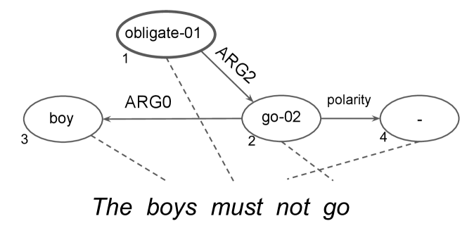
Figure 1: An example of AMR, the dashed lines denote latent alignments, obligate-01 is the root. Numbers indicate depth-first traversal order.

The semantic representations can be regarded as rooted labeled directed acyclic graphs (see Figure  1). As AMR abstracts away from details of surface realization, it is potentially beneficial in many semantic related NLP tasks, including text summarization Liu et al. (2015); Dohare and Karnick (2017), machine translation Jones et al. (2012) and question answering Mitra and Baral (2016).

AMR parsing has recently received a lot of attention (e.g., Flanigan et al. (2014); Artzi et al. (2015); Konstas et al. (2017)). One distinctive aspect of AMR annotation is the lack of explicit alignments between nodes in the graph (concepts) and words in the sentences. Though this arguably simplified the annotation process Banarescu et al. (2013), it is not straightforward to produce an effective parser without relying on an alignment. Most AMR parsers Damonte et al. (2017); Flanigan et al. (2016); Werling et al. (2015); Wang and Xue (2017); Foland and Martin (2017) use a pipeline where the aligner training stage precedes training a parser. The aligners are not directly informed by the AMR parsing objective and may produce alignments suboptimal for this task.

In this work, we demonstrate that the alignments can be treated as latent variables in a joint probabilistic model and induced in such a way as to be beneficial for AMR parsing. Intuitively, in our probabilistic model, every node in a graph is assumed to be aligned to a word in a sentence: each concept is predicted based on the corresponding RNN state. Similarly, graph edges (i.e. relations) are predicted based on representations of concepts and aligned words (see Figure 2). As alignments are latent, exact inference requires marginalizing over latent alignments, which is infeasible. Instead we use variational inference, specifically the variational autoencoding framework of Kingma and Welling (2014). Using discrete latent variables in deep learning has proven to be challenging Mnih and Gregor (2014); Bornschein and Bengio (2015). We use a continuous relaxation of the alignment problem, relying on the recently introduced Gumbel-Sinkhorn construction Mena et al. (2018). This yields a computationally-efficient approximate method for estimating our joint probabilistic model of concepts, relations and alignments.

We assume injective alignments from concepts to words: every node in the graph is aligned to a single word in the sentence and every word is aligned to at most one node in the graph. This is necessary for two reasons. First, it lets us treat concept identification as sequence tagging at test time. For every word we would simply predict the corresponding concept or predict NULL to signify that no concept should be generated at this position. Secondly, Gumbel-Sinkhorn can only work under this assumption. This constraint, though often appropriate, is problematic for certain AMR constructions (e.g., named entities). In order to deal with these cases, we re-categorized AMR concepts. Similar recategorization strategies have been used in previous work Foland and Martin (2017); Peng et al. (2017).

The resulting parser achieves 74.4% Smatch score on the standard test set when using LDC2016E25 training set, an improvement of 3.4% over the previous best result van Noord and Bos (2017). We also demonstrate that inducing alignments within the joint model is indeed beneficial. When, instead of inducing alignments, we follow the standard approach and produce them on preprocessing, the performance drops by 0.9% Smatch. Our main contributions can be summarized as follows:

• we introduce a joint probabilistic model for alignment, concept and relation identification;

• we demonstrate that a continuous relaxation can be used to effectively estimate the model;

• the model achieves the best reported results.

2 Probabilistic Model

In this section we describe our probabilistic model and the estimation technique. In section 3, we describe preprocessing and post-processing (including concept re-categorization, sense disambiguation, wikification and root selection).

2.1 Notation and setting

We will use the following notation throughout the paper. We refer to words in the sentences as $\mathbf{w}=(w_{1},\ldots,w_{n})$, where $n$ is sentence length, $w_{k}\in\mathcal{V}$ for $k\in\{1\ldots,n\}$. The concepts (i.e. labeled nodes) are $\mathbf{c}=(c_{1},\ldots,c_{m})$, where $m$ is the number of concepts and $c_{i}\in\mathcal{C}$ for $i\in\{1\ldots,m\}$. For example, in Figure 1, $\mathbf{c}=(\mbox{\it obligate},\mbox{\it go},\mbox{\it boy},\mbox{\it-})$. Note that senses are predicted at post-processing, as discussed in Section 3.2 (i.e. go is labeled as go-02).

A relation between ‘predicate concept’ $i$ and ‘argument concept’ $j$ is denoted by $r_{ij}\in\mathcal{R}$; it is set to NULL if $j$ is not an argument of $i$. In our example, $r_{2,3}=\mbox{\it ARG0}$ and $r_{1,3}=\mbox{\it NULL}$. We will use $R$ to denote all relations in the graph.

To represent alignments, we will use $\mathbf{a}=\{a_{1},\ldots,a_{m}\}$, where $a_{i}\in\{1,\ldots,n\}$ returns the index of a word aligned to concept $i$. In our example, $a_{1}=3$.

All three model components rely on bi-directional LSTM encoders Schuster and Paliwal (1997). We denote states of BiLSTM (i.e. concatenation of forward and backward LSTM states) as $\mathbf{h}_{k}\in\mathbb{R}^{d}$ ($k\in\{1,\ldots,n\}$). The sentence encoder takes pre-trained fixed word embeddings, randomly initialized lemma embeddings, part-of-speech and named-entity tag embeddings.

2.2 Method overview

Figure 2: Relation identification: predicting a relation between boy and go-02 relying on the two concepts and corresponding RNN states.

We believe that using discrete alignments, rather than attention-based models  Bahdanau et al. (2015) is crucial for AMR parsing. AMR banks are a lot smaller than parallel corpora used in machine translation (MT) and hence it is important to inject a useful inductive bias. We constrain our alignments from concepts to words to be injective. First, it encodes the observation that concepts are mostly triggered by single words (especially, after re-categorization, Section 3.1). Second, it implies that each word corresponds to at most one concept (if any). This encourages competition: alignments are mutually-repulsive. In our example, obligate is not lexically similar to the word must and may be hard to align. However, given that other concepts are easy to predict, alignment candidates other than must and the will be immediately ruled out. We believe that these are the key reasons for why attention-based neural models do not achieve competitive results on AMR Konstas et al. (2017) and why state-of-the-art models rely on aligners. Our goal is to combine best of two worlds: to use alignments (as in state-of-the-art AMR methods) and to induce them while optimizing for the end goal (similarly to the attention component of encoder-decoder models).

Our model consists of three parts: (1) the concept identification model $P_{\theta}(\mathbf{c}|\mathbf{a},\mathbf{w})$; (2) the relation identification model $P_{\phi}(R|\mathbf{a},\mathbf{w},\mathbf{c})$ and (3) the alignment model $Q_{\psi}(\mathbf{a}|\mathbf{c},R,\mathbf{w})$. Formally, (1) and (2) together with the uniform prior over alignments $P(\mathbf{a})$ form the generative model of AMR graphs. In contrast, the alignment model $Q_{\psi}(\mathbf{a}|\mathbf{c},R,\mathbf{w})$, as will be explained below, is approximating the intractable posterior $P_{\theta,\phi}(\mathbf{a}|\mathbf{c},R,\mathbf{w})$ within that probabilistic model.

In other words, we assume the following model for generating the AMR graph:

$$P_{\theta,\phi}(\mathbf{c},R|\mathbf{w})\!=\!\sum_{\!\mathbf{a}}{\!P(\mathbf{a})P_{\theta}(\mathbf{c}|\mathbf{a},\mathbf{w})P_{\phi}(R|\mathbf{a},\mathbf{w},\mathbf{c})}$$

$$=\!\sum_{\mathbf{a}}{\!P(\mathbf{a})\prod_{i=1}^{m}\!P(c_{i}|{\mathbf{h}_{a_{i}}})}\!\!\prod_{i,j=1}^{m}{\!\ P(r_{ij}|\mathbf{h}_{a_{i}},\!\mathbf{c}_{i},\!\mathbf{h}_{a_{j}},\!\mathbf{c}_{j})}$$

AMR concepts are assumed to be generated conditional independently relying on the BiLSTM states and surface forms of the aligned words. Similarly, relations are predicted based only on AMR concept embeddings and LSTM states corresponding to words aligned to the involved concepts. Their combined representations are fed into a bi-affine classifier Dozat and Manning (2017) (see Figure 2).

The expression involves intractable marginalization over all valid alignments. As standard in variational autoencoders, VAEs Kingma and Welling (2014), we lower-bound the log-likelihood as

$$\log P_{\theta,\phi}(\mathbf{c},R|\mathbf{w})$$

$$\geq E_{Q}[\log P_{\theta}(\mathbf{c}|\mathbf{a},\mathbf{w})P_{\phi}(R|\mathbf{a},\mathbf{w},\mathbf{c})]$$

$$-D_{KL}(Q_{\psi}(\mathbf{a}|\mathbf{c},R,\mathbf{w})||P(\mathbf{a})),$$ (1)

where $Q_{\psi}(\mathbf{a}|\mathbf{c},R,\mathbf{w})$ is the variational posterior (aka the inference network), $E_{Q}[\ldots]$ refers to the expectation under $Q_{\psi}(\mathbf{a}|\mathbf{c},R,\mathbf{w})$ and $D_{KL}$ is the Kullback-Liebler divergence. In VAEs, the lower bound is maximized both with respect to model parameters ($\theta$ and $\phi$ in our case) and the parameters of the inference network ($\psi$). Unfortunately, gradient-based optimization with discrete latent variables is challenging. We use a continuous relaxation of our optimization problem, where real-valued vectors $\hat{\mathbf{a}}_{i}\in\mathbb{R}^{n}$ (for every concept $i$) approximate discrete alignment variables $a_{i}$. This relaxation results in low-variance estimates of the gradient using the parameterization trick Kingma and Welling (2014), and ensures fast and stable training. We will describe the model components and the relaxed inference procedure in detail in sections 2.6 and 2.7.

Though the estimation procedure requires the use of the relaxation, the learned parser is straightforward to use. Given our assumptions about the alignments, we can independently choose for each word $w_{k}$ ($k=1,\ldots,m$) the most probably concept according to $P_{\theta}(c|\mathbf{h}_{k})$. If the highest scoring option is NULL, no concept is introduced. The relations could then be predicted relying on $P_{\phi}(R|\mathbf{a},\mathbf{w},\mathbf{c})$. This would have led to generating inconsistent AMR graphs, so instead we search for the highest scoring valid graph (see Section 3.2). Note that the alignment model $Q_{\psi}$ is not used at test time and only necessary to train accurate concept and relation identification models.

2.3 Concept identification model

The concept identification model chooses a concept $c$ (i.e. a labeled node) conditioned on the aligned word $k$ or decides that no concept should be introduced (i.e. returns NULL). Though it can be modeled with a softmax classifier, it would not be effective in handling rare or unseen words. First, we split the decision into estimating the probability of concept category $\tau(c)\in\mathcal{T}$ (e.g. ‘number’, ’frame’) and estimating the probability of the specific concept within the chosen category. Second, based on a lemmatizer and training data we prepare one candidate concept $e_{k}$ for each word $k$ in vocabulary (e.g., it would propose want if the word is wants). Similar to Luong et al. (2015), our model can then either copy the candidate $e_{k}$ or rely on the softmax over potential concepts of category $\tau$. Formally, the concept prediction model is defined as

$$P_{\theta}( c|\mathbf{h}_{k},w_{k})=P(\tau(c)|\mathbf{h}_{k},w_{k})\times$$

$$\frac{[[e_{k}=c]]\times\exp(\mathbf{v}_{copy}^{T}\mathbf{h_{k}})+\exp(\mathbf{v}_{c}^{T}\mathbf{h_{k}})}{Z(\mathbf{h_{k}},\theta)},$$

where the first multiplicative term is a softmax classifier over categories (including NULL); $\mathbf{v}_{copy},\mathbf{v}_{c}\in\mathbb{R}^{d}$ (for $c\in\mathcal{C}$) are model parameters; $[[\ldots]]$ denotes the indicator function and equals 1 if its argument is true and 0, otherwise; $Z(\mathbf{h},\theta)$ is the partition function ensuring that the scores sum to 1.

2.4 Relation identification model

We use the following arc-factored relation identification model:

$$P_{\phi}(R|\mathbf{a},\mathbf{w},\mathbf{c})=\prod_{i,j=1}^{m}{\!\ P(r_{ij}|\mathbf{h}_{a_{i}},\!\mathbf{c}_{i},\!\mathbf{h}_{a_{j}},\!\mathbf{c}_{j})}$$ (2)

Each term is modeled in exactly the same way:

1. for both endpoints, embedding of the concept $c$ is concatenated with the RNN state $\mathbf{h}$;

2. they are linearly projected to a lower dimension separately through $M_{h}(\mathbf{h}_{a_{i}}\circ c_{i})\in\mathbb{R}^{d_{f}}$ and $M_{d}(\mathbf{h}_{a_{j}}\circ c_{j})\in\mathbb{R}^{d_{f}}$, where $\circ$ denotes concatenation;

3. a log-linear model with bilinear scores $M_{h}(\mathbf{h}_{a_{i}}\circ c_{i})^{T}C_{r}M_{d}(\mathbf{h}_{a_{j}}\circ c_{j})$, $C_{r}\in\mathbb{R}^{d_{f}\times d_{f}}$ is used to compute the probabilities.

In the above discussion, we assumed that BiLSTM encodes a sentence once and the BiLSTM states are then used to predict concepts and relations. In semantic role labeling, the task closely related to the relation identification stage of AMR parsing, a slight modification of this approach was shown more effective Zhou and Xu (2015); Marcheggiani et al. (2017). In that previous work, the sentence was encoded by a BiLSTM once per each predicate (i.e. verb) and the encoding was in turn used to identify arguments of that predicate. The only difference across the re-encoding passes was a binary flag used as input to the BiLSTM encoder at each word position. The flag was set to 1 for the word corresponding to the predicate and to 0 for all other words. In that way, BiLSTM was encoding the sentence specifically for predicting arguments of a given predicate. Inspired by this approach, when predicting label $r_{ij}$ for $j\in\{1,\ldots\,m\}$, we input binary flags $\mathbf{p}_{1},\ldots\mathbf{p}_{n}$ to the BiLSTM encoder which are set to $1$ for the word indexed by $a_{i}$ ($\mathbf{p}_{a_{i}}=1$) and to $0$ for other words ($\mathbf{p}_{j}=0$, for $j\neq a_{i}$). This also means that BiLSTM encoders for predicting relations and concepts end up being distinct. We use this multi-pass approach in our experiments.

2.5 Alignment model

Recall that the alignment model is only used at training, and hence it can rely both on input (states $\mathbf{h}_{1},\ldots,\mathbf{h}_{n}$) and on the list of concepts $c_{1},\ldots,c_{m}$.

Formally, we add $(m-n)$ NULL concepts to the list. Aligning a word to any NULL, would correspond to saying that the word is not aligned to any ‘real’ concept. Note that each one-to-one alignment (i.e. permutation) between $n$ such concepts and $n$ words implies a valid injective alignment of $n$ words to $m$ ‘real’ concepts. This reduction to permutations will come handy when we turn to the Gumbel-Sinkhorn relaxation in the next section. Given this reduction, from now on, we will assume that $m=n$.

As with sentences, we use a BiLSTM model to encode concepts $\mathbf{c}$, where $\mathbf{g}_{i}\in\mathcal{R}^{d_{g}}$, $i\in\{1,\ldots,n\}$. We use a globally-normalized alignment model:

$$Q_{\psi}(\mathbf{a}|\mathbf{c},R,\mathbf{w})=\frac{\exp(\sum_{i=1}^{n}{\varphi(\mathbf{g}_{i},\mathbf{h}_{a_{i}})})}{Z_{\psi}(\mathbf{c},\mathbf{w})},$$

where $Z_{\psi}(\mathbf{c},\mathbf{w})$ is the intractable partition function and the terms $\varphi(\mathbf{g}_{i},\mathbf{h}_{a_{i}})$ score each alignment link according to a bilinear form

$$\varphi(\mathbf{g}_{i},\mathbf{h}_{a_{i}})=\mathbf{g}_{i}^{T}B\mathbf{h}_{a_{i}},$$ (3)

where $B\in\mathbb{R}^{d_{g}\times d}$ is a parameter matrix.

2.6 Estimating model with Gumbel-Sinkhorn

Recall that our learning objective (1) involves expectation under the alignment model. The partition function of the alignment model $Z_{\psi}(\mathbf{c},\mathbf{w})$ is intractable, and it is tricky even to draw samples from the distribution. Luckily, the recently proposed relaxation Mena et al. (2018) lets us circumvent this issue. First, note that exact samples from a categorical distribution can be obtained using the perturb-and-max technique Papandreou and Yuille (2011). For our alignment model, it would correspond to adding independent noise to the score for every possible alignment and choosing the highest scoring one:

$$\mathbf{a^{\star}}=\operatorname*{argmax}_{\mathbf{a}\in\mathcal{P}}{\sum_{i=1}^{n}{\varphi(\mathbf{g}_{i},\mathbf{h}_{a_{i}})}+\epsilon_{\mathbf{a}}},$$ (4)

where $\mathcal{P}$ is the set of all permutations of $n$ elements, $\epsilon_{\mathbf{a}}$ is a noise drawn independently for each $\mathbf{a}$ from the fixed Gumbel distribution ($\mathcal{G}(0,1)$). Unfortunately, this is also intractable, as there are $n!$ permutations. Instead, in perturb-and-max an approximate schema is used where noise is assumed factorizable. In other words, first noisy scores are computed as $\hat{\varphi}(\mathbf{g}_{i},\mathbf{h}_{a_{i}})={\varphi}(\mathbf{g}_{i},\mathbf{h}_{a_{i}})+\epsilon_{i,a_{i}}$, where $\epsilon_{i,a_{i}}\sim\mathcal{G}(0,1)$ and an approximate sample is obtained by $\mathbf{a^{\star}}=\operatorname*{argmax}_{\mathbf{a}}{\sum_{i=1}^{n}{\hat{\varphi}(\mathbf{g}_{i},\mathbf{h}_{a_{i}})}},$

Such sampling procedure is still intractable in our case and also non-differentiable. The main contribution of Mena et al. (2018) is approximating this $\operatorname*{argmax}$ with a simple differentiable computation $\hat{\mathbf{a}}=S_{t}(\Phi,\Sigma)$ which yields an approximate (i.e. relaxed) permutation. We use $\Phi$ and $\Sigma$ to denote the $n\times n$ matrices of alignment scores $\varphi(\mathbf{g}_{i},\mathbf{h}_{k})$ and noise variables $\epsilon_{ik}$, respectively. Instead of returning index $a_{i}$ for every concept $i$, it would return a (peaky) distribution over words $\hat{\mathbf{a}}_{i}$. The peakiness is controlled by the temperature parameter $t$ of Gumbel-Sinkhorn which balances smoothness (‘differentiability’) vs. bias of the estimator. For further details and the derivation, we refer the reader to the original paper  Mena et al. (2018).

Note that $\Phi$ is a function of the alignment model $Q_{\psi}$, so we will write $\Phi_{\psi}$ in what follows. The variational bound (1) can now be approximated as

$$E_{\Sigma\sim\mathcal{G}(0,1)}[\log P_{\theta}(c|S_{t}(\Phi_{\psi},\Sigma),\mathbf{w})$$

$$\quad+\log P_{\phi}(R|S_{t}(\Phi_{\psi},\Sigma),\mathbf{w},\mathbf{c})]$$

$$\quad-D_{KL}(\frac{\Phi_{\psi}+\Sigma}{t}||\frac{\Sigma}{t_{0}})$$ (5)

Following  Mena et al. (2018), the original KL term from equation (1) is approximated by the KL term between two $n\times n$ matrices of i.i.d. Gumbel distributions with different temperature and mean. The parameter $t_{0}$ is the ‘prior temperature’.

Using the Gumbel-Sinkhorn construction unfortunately does not guarantee that $\sum_{i}\hat{\mathbf{a}}_{ij}=1$. To encourage this equality to hold, and equivalently to discourage overlapping alignments, we add another regularizer to the objective (5):

$$\Omega(\hat{\mathbf{a}},\lambda)=\lambda\sum_{j}\max(\sum_{i}(\hat{\mathbf{a}}_{ij})-1,0).$$ (6)

Our final objective is fully differentiable with respect to all parameters (i.e. $\theta$, $\phi$ and $\psi$) and has low variance as sampling is performed from the fixed non-parameterized distribution, as in standard VAEs.

2.7 Relaxing concept and relation identification

One remaining question is how to use the soft input $\hat{\mathbf{a}}=S_{t}(\Phi_{\psi},\Sigma)$ in the concept and relation identification models in equation (5). In other words, we need to define how we compute $P_{\theta}(c|S_{t}(\Phi_{\psi},\Sigma),\mathbf{w})$ and $P_{\phi}(R|S_{t}(\Phi_{\psi},\Sigma),\mathbf{w},\mathbf{c})$.

The standard technique would be to pass to the models expectations under the relaxed variables $\sum_{k=1}^{n}{\hat{\mathbf{a}}_{ik}\mathbf{h}_{k}}$, instead of the vectors $\mathbf{h}_{a_{i}}$ Maddison et al. (2017); Jang et al. (2017). This is what we do for the relation identification model. We use this approach also to relax the one-hot encoding of the predicate position ($\mathbf{p}$, see Section 2.4).

However, the concept prediction model $\log P_{\theta}(c|S_{t}(\Phi_{\psi},\Sigma),\mathbf{w})$ relies on the pointing mechanism, i.e. directly exploits the words $\mathbf{w}$ rather than relies only on biLSTM states $\mathbf{h}_{k}$. So instead we treat $\hat{\mathbf{a}}_{i}$ as a prior in a hierarchical model:

$$\log P_{\theta}(c_{i}|\mathbf{\hat{a}_{i}},\mathbf{w})$$

$$\approx\log\sum_{k=1}^{n}{\hat{\mathbf{a}}_{ik}P_{\theta}(c_{i}|a_{i}=k,\mathbf{w})}$$ (7)

As we will show in our experiments, a softer version of the loss is even more effective:

$$\log P_{\theta}(c_{i}|\mathbf{\hat{a}_{i}},\mathbf{w})$$

$$\approx{\log\sum_{k=1}^{n}{(\hat{\mathbf{a}}_{ik}P_{\theta}(c_{i}|a_{i}=k,\mathbf{w}))^{\alpha}}},$$ (8)

where we set the parameter $\alpha=0.5$. We believe that using this loss encourages the model to more actively explore the alignment space. Geometrically, the loss surface shaped as a ball in the 0.5-norm space would push the model away from the corners, thus encouraging exploration.

3 Pre- and post-pocessing

3.1 Re-Categorization

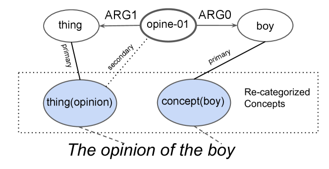
Figure 3: An example of re-categorized AMR. AMR graph at the top, re-categorized concepts in the middle, and the sentence is at the bottom.

AMR parsers often rely on a pre-processing stage, where specific subgraphs of AMR are grouped together and assigned to a single node with a new compound category (e.g., Werling et al. (2015); Foland and Martin (2017); Peng et al. (2017)); this transformation is reversed at the post-processing stage. Our approach is very similar to the Factored Concept Label system of  Wang and Xue (2017), with one important difference that we unpack our concepts before the relation identification stage, so the relations are predicted between original concepts (all nodes in each group share the same alignment distributions to the RNN states). Intuitively, the goal is to ensure that concepts rarely lexically triggered (e.g., thing in Figure 3) get grouped together with lexically triggered nodes. Such ‘primary’ concepts get encoded in the category of the concept (the set of categories is $\mathcal{\tau}$, see also section 2.3). In Figure 3, the re-categorized concept thing(opinion) is produced from thing and opine-01. We use concept as the dummy category type. There are 8 templates in our system which extract re-categorizations for fixed phrases (e.g. thing(opinion)), and a deterministic system for grouping lexically flexible, but structurally stable sub-graphs (e.g., named entities, have-rel-role-91 and have-org-role-91 concepts).

Details of the re-categorization procedure and other pre-processing are provided in appendix.

3.2 Post-processing

For post-processing, we handle sense-disambiguation, wikification and ensure legitimacy of the produced AMR graph. For sense disambiguation we pick the most frequent sense for that particular concept (‘-01’, if unseen). For wikification we again look-up in the training set and default to ”-”. There is certainly room for improvement in both stages. Our probability model predicts edges conditional independently and thus cannot guarantee the connectivity of AMR graph, also there are additional constraints which are useful to impose. We enforce three constraints: (1) specific concepts can have only one neighbor (e.g., ‘number’ and ‘string’; see appendix for details); (2) each predicate concept can have at most one argument for each relation $r\in\mathcal{R}$; (3) the graph should be connected. Constraint (1) is addressed by keeping only the highest scoring neighbor. In order to satisfy the last two constraints we use a simple greedy procedure. First, for each edge, we pick-up the highest scoring relation and edge (possibly NULL). If the constraint (2) is violated, we simply keep the highest scoring edge among the duplicates and drop the rest. If the graph is not connected (i.e. constraint (3) is violated), we greedily choose edges linking the connected components until the graph gets connected (MSCG in Flanigan et al. (2014)).

Finally, we need to select a root node. Similarly to relation identification, for each candidate concept $c_{i}$, we concatenate its embedding with the corresponding LSTM state ($\mathbf{h}_{a_{i}}$) and use these scores in a softmax classifier over all the concepts.

4 Experiments and Discussion

4.1 Data and setting

We primarily focus on the most recent LDC2016E25 (R2) dataset, which consists of 36521, 1368 and 1371 sentences in training, development and testing sets, respectively. The earlier LDC2015E86 (R1) dataset has been used by much of the previous work. It contains 16833 training sentences, and same sentences for development and testing as R2.

We used the development set to perform model selection and hyperparameter tuning. The hyperparameters, as well as information about embeddings and pre-processing, are presented in the supplementary materials.

We used Adam Kingma and Ba (2014) to optimize the loss (5) and to train the root classifier. Our best model is trained fully jointly, and we do early stopping on the development set scores. Training takes approximately 6 hours on a single GeForce GTX 1080 Ti with Intel Xeon CPU E5-2620 v4.

Model	Data	Smatch
JAMR Flanigan et al. (2016)	R1	67.0
AMREager Damonte et al. (2017)	R1	64.0
CAMR Wang et al. (2016)	R1	66.5
SEQ2SEQ + 20M Konstas et al. (2017)	R1	62.1
Mul-BiLSTM Foland and Martin (2017)	R1	70.7
Ours	R1	73.7
Neural-Pointer Buys and Blunsom (2017)	R2	61.9
ChSeq van Noord and Bos (2017)	R2	64.0
ChSeq + 100K van Noord and Bos (2017)	R2	71.0
Ours	R2	74.4 $\pm$ 0.16

Table 1: Smatch scores on the test set. R2 is LDC2016E25 dataset, and R1 is LDC2015E86 dataset. Statistics on R2 are over 8 runs.

4.2 Experiments and discussion

We start by comparing our parser to previous work (see Table  1). Our model substantially outperforms all the previous models on both datasets. Specifically, it achieves 74.4% Smatch score on LDC2016E25 (R2), which is an improvement of 3.4% over character seq2seq model relying on silver data van Noord and Bos (2017). For LDC2015E86 (R1), we obtain 73.7% Smatch score, which is an improvement of 3.0% over the previous best model, multi-BiLSTM parser of Foland and Martin (2017).

Models	A’	C’	J’	Ch’	Ours
	17	16	16	17
Dataset	R1	R1	R1	R2	R2
Smatch	64	63	67	71	74.4$\pm 0.16$
Unlabeled	69	69	69	74	77.1$\pm 0.10$
No WSD	65	64	68	72	75.5$\pm 0.12$
Reentrancy	41	41	42	52	52.3$\pm 0.43$
Concepts	83	80	83	82	85.9$\pm 0.11$
NER	83	75	79	79	86.0$\pm 0.46$
Wiki	64	0	75	65	75.7$\pm 0.30$
Negations	48	18	45	62	58.4$\pm 1.32$
SRL	56	60	60	66	69.8$\pm 0.24$

Table 2: F1 scores on individual phenomena. A’17 is AMREager, C’16 is CAMR, J’16 is JAMR, Ch’17 is ChSeq+100K. Ours are marked with standard deviation.

In order to disentangle individual phenomena, we use the AMR-evaluation tools Damonte et al. (2017) and compare to systems which reported these scores (Table 2). We obtain the highest scores on most subtasks. The exception is negation detection. However, this is not too surprising as many negations are encoded with morphology, and character models, unlike our word-level model, are able to capture predictive morphological features (e.g., detect prefixes such as “un-” or “im-”).

Metric	Pre-	R1	Pre-	R2
	Align		Align	mean
Smatch	72.8	73.7	73.5	74.4
Unlabeled	75.3	76.3	76.1	77.1
No WSD	73.8	74.7	74.6	75.5
Reentrancy	50.2	50.6	52.6	52.3
Concepts	85.4	85.5	85.5	85.9
NER	85.3	84.8	85.3	86.0
Wiki	66.8	75.6	67.8	75.7
Negations	56.0	57.2	56.6	58.4
SRL	68.8	68.9	70.2	69.8

Table 3: F1 scores of on subtasks. Scores on ablations are averaged over 2 runs. The left side results are from LDC2015E86 and right results are from LDC2016E25.

Now, we turn to ablation tests (see Table 3). First, we would like to see if our latent alignment framework is beneficial. In order to test this, we create a baseline version of our system (‘pre-align’) which relies on the JAMR aligner Flanigan et al. (2014), rather than induces alignments as latent variables. Recall that in our model we used training data and a lemmatizer to produce candidates for the concept prediction model (see Section 2.3, the copy function). In order to have a fair comparison, if a concept is not aligned after JAMR, we try to use our copy function to align it. If an alignment is not found, we make the alignment uniform across the unaligned words. In preliminary experiments, we considered alternatives versions (e.g., dropping concepts unaligned by JAMR or dropping concepts unaligned after both JAMR and the matching heuristic), but the chosen strategy was the most effective. These scores of pre-align are superior to the results from Foland and Martin (2017) which also relies on JAMR alignments and uses BiLSTM encoders. There are many potential reasons for this difference in performance. For example, their relation identification model is different (e.g., single pass, no bi-affine modeling), they used much smaller networks than us, they use plain JAMR rather than a combination of JAMR and our copy function, they use a different recategorization system. These results confirm that we started with a strong basic model, and that our variational alignment framework provided further gains in performance.

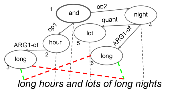
Figure 4: When modeling concepts alone, the posterior probability of the correct (green) and wrong (red) alignment links will be the same.

Ablation	Concepts	SRL	Smatch
2 stages	85.6	68.9	73.6
2 stages, tune align	85.6	69.2	73.9
Full model	85.9	69.8	74.4

Table 4: Ablation studies: effect of joint modeling (all on R2). Scores on ablations are averaged over 2 runs. The first two models load the same concept and alignment model before the second stage.

Now we would like to confirm that joint training of alignments with both concepts and relations is beneficial. In other words, we would like to see if alignments need to be induced in such a way as to benefit the relation identification task. For this ablation we break the full joint training into two stages. We start by jointly training the alignment model and the concept identification model. When these are trained, we optimizing the relation model but keep the concept identification model and alignment models fixed (‘2 stages’ in see Table 4). When compared to our joint model (‘full model’), we observe a substantial drop in Smatch score (-0.8%). In another version (‘2 stages, tune align’) we also use two stages but we fine-tune the alignment model on the second stage. This approach appears slightly more accurate but still -0.5% below the full model. In both cases, the drop is more substantial for relations (‘SRL’). In order to see why relations are potentially useful in learning alignments, consider Figure 4. The example contains duplicate concepts long. The concept prediction model factorizes over concepts and does not care which way these duplicates are aligned: correctly (green edges) or not (red edges). Formally, the true posterior under the concept-only model in ‘2 stages’ assigns exactly the same probability to both configurations, and the alignment model $Q_{\psi}$ will be forced to mimic it (even though it relies on an LSTM model of the graph). The spurious ambiguity will have a detrimental effect on the relation identification stage.

Ablation	Concepts	SRL	Smatch
No Sinkhorn	85.7	69.3	73.8
No Sinkhorn reg	85.6	69.5	74.2
No soft loss	85.2	69.1	73.7
Full model	85.9	69.8	74.4

Table 5: Ablation studies: alignment modeling and relaxation (all on R2). Scores on ablations are averaged over 2 runs.

It is interesting to see the contribution of other modeling decisions we made when modeling and relaxing alignments. First, instead of using Gumbel-Sinkhorn, which encourages mutually-repulsive alignments, we now use a factorized alignment model. Note that this model (‘No Sinkhorn’ in Table 5) still relies on (relaxed) discrete alignments (using Gumbel softmax) but does not constrain the alignments to be injective. A substantial drop in performance indicates that the prior knowledge about the nature of alignments appears beneficial. Second, we remove the additional regularizer for Gumbel-Sinkhorn approximation (equation (6)). The performance drop in Smatch score (‘No Sinkhorn reg’) is only moderate. Finally, we show that using the simple hierarchical relaxation (equation (7)) rather than our softer version of the loss (equation (8)) results in a substantial drop in performance (‘No soft loss’, -0.7% Smatch). We hypothesize that the softer relaxation favors exploration of alignments and helps to discover better configurations.

5 Additional Related Work

Alignment performance has been previously identified as a potential bottleneck affecting AMR parsing Damonte et al. (2017); Foland and Martin (2017). Some recent work has focused on building aligners specifically for training their parsers Werling et al. (2015); Wang and Xue (2017). However, those aligners are trained independently of concept and relation identification and only used at pre-processing.

Treating alignment as discrete variables has been successful in some sequence transduction tasks with neural models Yu et al. (2017, 2016). Our work is similar in that we also train discrete alignments jointly but the tasks, the inference framework and the decoders are very different.

The discrete alignment modeling framework has been developed in the context of traditional (i.e. non-neural) statistical machine translation Brown et al. (1993). Such translation models have also been successfully applied to semantic parsing tasks (e.g., Andreas et al. (2013)), where they rivaled specialized semantic parsers from that period. However, they are considerably less accurate than current state-of-the-art parsers applied to the same datasets (e.g., Dong and Lapata (2016)).

For AMR parsing, another way to avoid using pre-trained aligners is to use seq2seq models Konstas et al. (2017); van Noord and Bos (2017). In particular, van Noord and Bos (2017) used character level seq2seq model and achieved the previous state-of-the-art result. However, their model is very data demanding as they needed to train it on additional 100K sentences parsed by other parsers. This may be due to two reasons. First, seq2seq models are often not as strong on smaller datasets. Second, recurrent decoders may struggle with predicting the linearized AMRs, as many statistical dependencies are highly non-local.

6 Conclusions

We introduced a neural AMR parser trained by jointly modeling alignments, concepts and relations. We make such joint modeling computationally feasible by using the variational auto-encoding framework and continuous relaxations. The parser achieves state-of-the-art results and ablation tests show that joint modeling is indeed beneficial.

We believe that the proposed approach may be extended to other parsing tasks where alignments are latent (e.g., parsing to logical form Liang (2016)). Another promising direction is integrating character seq2seq to substitute the copy function. This should also improve the handling of negation and rare words. Though our parsing model does not use any linearization of the graph, we relied on LSTMs and somewhat arbitrary linearization (depth-first traversal) to encode the AMR graph in our alignment model. A better alternative would be to use graph convolutional networks Marcheggiani and Titov (2017); Kipf and Welling (2017): neighborhoods in the graph are likely to be more informative for predicting alignments than the neighborhoods in the graph traversal.

Supplementary Material

7 Matching algorithm for copying concepts

Only frequent concepts $c$ (frequency at least 10 for R2 and 5 for R1) can be generated without the copying mechanism (i.e. have their own vector $\mathbf{v}_{c}$ associated with them). Both frequent and infrequent ones are processed with coping, using candidates produced by the algorithm below and the matching rule in Table 6.

Input :  $\{\mathbf{w}^{l},\mathbf{c}^{l}\}^{L}_{l=1}$

Output :  D copy dictionary

Counter $\leftarrow\emptyset$

for $l=1$ to $L$ do

       for all pairs $c_{i}^{l}$ and $w_{j}^{l}$ do

             if  match($c_{i}^{l}$, $w_{j}^{l}$) then

                   Increment Counter[$w_{j}^{l}$][$c_{i}^{l}$]

             end if

            

       end for

      

end for

D $\leftarrow$ default Stanford lemmatizer

for w $\leftarrow$ Counter do

       D[w] $\leftarrow\operatorname*{argmax}_{c}$ Counter[w][c]

end for

return D

Algorithm 1 Copy function construction

Rules	Matching Criteria
Verbalization Match	exact match frame in ”verbalization-list-v1.06.txt”
PropBank Match	exact match frame in PropBank frame files
Suffix Removal Match	word with suffix (“-ed”, “-ly”,“-ing”) removed is identical to concept lemma
Edit-distance Match	edit distance smaller than 50% of the length

Table 6: Matching rules for Algorithm 1

8 Re-categorization details

Re-categorization is handled with rules listed in Table 2. They are triggered if a given primary concept (‘primary’) appears adjacent to edges labeled with relations given in column ‘rel’. The assigned category is shown in column ‘re-categorized’. The rules yield 32 categories when applied to the training set.

primary	rel	re-categorized
person	ARG0-of/ARG1-of	person([second])
thing	ARG0-of/ARG1-of/ARG2-of	thing([second])
most	degree-of	most([second])
-quantity	unit	primary([second])
date-entity	weekday/dayperiod/season	date-entity([second])
monetary-quantity	unit/ARG2-of/ARG1-of/quant	monetary-quantity([second])
temporal-quantity	unit/ARG3-of	temporal-quantity([second])

Table 7: Templates for re-categorization.

There are also rules of another type shown in Table 3 below. The templates and examples are in column ‘original’, the resulting concepts are in column ‘re-categorized’. These rules yield 109 additional types when applied to the training set.

original	re-categorized
⬇ (c / type :name (n / name :op1 ‘n1’ … :opx ‘nx’)	(B-Ner_type(n1),…,Ner_type(nx))
⬇ (c / city :name (n / name :op1 ‘New’ :op2 ‘York’)	B-Ner_city(New),Ner_city(York)
⬇ (p / type :ARG0-of (h / have-x-role-91 :ARG2 (p / role)	have-x-role_type(role)
⬇ (p / person :ARG0-of (h / have-org-role-91 :ARG2 (p / premier)	have-org-role_person(premier)
⬇ (o1 / x-entity :x constant)	x-entity(constant)
⬇ (o1 / ordinal-entity :value 1)	ordinal-entity(1)

Table 8: Extra rules for re-categorization.

9 Additional pre-processing

Besides constructing re-categorized AMR concepts, we perform additional preprocessing. We start with tokenized dataset of Pourdamghani et al. (2014). We take all dashed AMR concepts (e.g, make-up and more-than) and concatenate the corresponding spans (based on statistics from training set and PropBank frame files). We also combine spans of words corresponding to a single number. For relation identification, we normalize relations to one canonical direction (e.g. arg0, time-of). For named entity recognition, and lemmatization, we use Stanford CoreNLP toolkit Manning et al. (2014). For pre-trained embedding, we used Glove (300 dimensional embeddings) Pennington et al. (2014).

10 Model parameters and optimization details

We selected hyper-parameters based on the best performance on the development set. For all the ablation tests, the hyper parameters are fixed. We used 2 different BiLSTM encoders of the same hyper-parameters to encode sentence for concept identification and alignment prediction, another BiLSTM to encode AMR concept sequence for alignment, and finally 2 different BiLSTM of the same hyper-parameters to encode sentence for relation identification and root identification. There are 5 BiLSTM encoders in total. Hyper parameters for the model are summarized in Table 9, and optimization parameters are summarized in Table 10.

Model components	Hyper-parameters
Glove Embeddings	300
Lemma Embeddings	200
POS Embeddings	32
NER Embeddings	16
Category Embeddings	32
Concept/Alignment	1 layer 548 input
Sentence BiLSTM	256 hidden (each direction)
AMR Categories $\mathcal{T}$	32
AMR Lemmas $\mathcal{C}$	506
AMR NER types	109
Alignment	1 layer 232 input
AMR BiLSTM	100 hidden (each direction)
$B$ bilinear align	200 $\times$ 512
Relation map dimensionality $d_{g}$	200
Relation/Root	2 layers 549 input (predicate position)
Sentence BiLSTM	256 hidden (each direction)
$d_{f}$ relation vector	200
$v_{c},v_{copy}$ lemma vector	512
$v_{root}$ root vector	200
Sinkhorn temperature	1
Sinkhorn prior temperature	5
Sinkhorn steps l for full joint training	10
Sinkhorn steps l for two stages training	5
$\lambda$	10
Dropout	.2

Table 9: Model hyper-parameters

Optimizer Parameters	Values
Batch size for single stage	64
Maximum Epochs	30
Batch size for first stage	512
Batch size for second stage	64
Maximum Epochs for both stages	30
Learning Rate	1e-4
Adam betas	(0.9, 0.999)
Adam eps	1e-8
Weight decay	1e-5

Table 10: Optimization parameters for full joint training and two stages training.

References

- Andreas et al. (2013) Jacob Andreas, Andreas Vlachos, and Stephen Clark. 2013. Semantic parsing as machine translation. In Proceedings of the 51st Annual Meeting of the Association for Computational Linguistics (Volume 2: Short Papers), volume 2, pages 47–52.
- Artzi et al. (2015) Yoav Artzi, Kenton Lee, and Luke Zettlemoyer. 2015. Broad-coverage CCG semantic parsing with AMR. In Proceedings of the 2015 Conference on Empirical Methods in Natural Language Processing, pages 1699–1710.
- Bahdanau et al. (2015) Dzmitry Bahdanau, Kyunghyun Cho, and Yoshua Bengio. 2015. Neural machine translation by jointly learning to align and translate. International Conference on Learning Representations.
- Banarescu et al. (2013) Laura Banarescu, Claire Bonial, Shu Cai, Madalina Georgescu, Kira Griffitt, Ulf Hermjakob, Kevin Knight, Philipp Koehn, Martha Palmer, and Nathan Schneider. 2013. Abstract Meaning Representation for Sembanking.
- Bornschein and Bengio (2015) Jörg Bornschein and Yoshua Bengio. 2015. Reweighted wake-sleep. International Conference on Learning Representations.
- Brown et al. (1993) Peter F. Brown, Vincent J. Della Pietra, Stephen A. Della Pietra, and Robert L. Mercer. 1993. The mathematics of statistical machine translation: Parameter estimation. Comput. Linguist., 19(2):263–311.
- Buys and Blunsom (2017) Jan Buys and Phil Blunsom. 2017. Oxford at semeval-2017 task 9: Neural amr parsing with pointer-augmented attention. In Proceedings of the 11th International Workshop on Semantic Evaluation (SemEval-2017), pages 914–919. Association for Computational Linguistics.
- Damonte et al. (2017) Marco Damonte, Shay B Cohen, and Giorgio Satta. 2017. An Incremental Parser for Abstract Meaning Representation. In Proceedings of the 15th Conference of the European Chapter of the Association for Computational Linguistics: Volume 1, Long Papers, volume 1, pages 536–546.
- Dohare and Karnick (2017) Shibhansh Dohare and Harish Karnick. 2017. Text Summarization using Abstract Meaning Representation. arXiv preprint arXiv:1706.01678.
- Dong and Lapata (2016) Li Dong and Mirella Lapata. 2016. Language to logical form with neural attention. In Proceedings of the 54th Annual Meeting of the Association for Computational Linguistics (Volume 1: Long Papers), volume 1, pages 33–43.
- Dozat and Manning (2017) Timothy Dozat and Christopher D. Manning. 2017. Deep Biaffine Attention for Neural Dependency Parsing. International Conference on Learning Representations.
- Flanigan et al. (2016) Jeffrey Flanigan, Chris Dyer, Noah A. Smith, and Jaime Carbonell. 2016. CMU at SemEval-2016 Task 8: Graph-based AMR Parsing with Infinite Ramp Loss. In Proceedings of the 10th International Workshop on Semantic Evaluation (SemEval-2016), pages 1202–1206. Association for Computational Linguistics.
- Flanigan et al. (2014) Jeffrey Flanigan, Sam Thomson, Jaime Carbonell, Chris Dyer, and Noah A. Smith. 2014. A Discriminative Graph-Based Parser for the Abstract Meaning Representation. In Proceedings of the 52nd Annual Meeting of the Association for Computational Linguistics (Volume 1: Long Papers), pages 1426–1436, Baltimore, Maryland. Association for Computational Linguistics.
- Foland and Martin (2017) William Foland and James H. Martin. 2017. Abstract Meaning Representation Parsing using LSTM Recurrent Neural Networks. In Proceedings of the 55th Annual Meeting of the Association for Computational Linguistics (Volume 1: Long Papers), pages 463–472, Vancouver, Canada. Association for Computational Linguistics.
- Jang et al. (2017) Eric Jang, Shixiang Gu, and Ben Poole. 2017. Categorical reparameterization with gumbel-softmax. International Conference on Learning Representations.
- Jones et al. (2012) Bevan K. Jones, Jacob Andreas, Daniel Bauer, Karl Moritz Hermann, and Kevin Knight. 2012. Semantics-Based Machine Translation with Hyperedge Replacement Grammars. In COLING.
- Kingma and Ba (2014) Diederik P. Kingma and Jimmy Ba. 2014. Adam: A Method for Stochastic Optimization. International Conference on Learning Representations.
- Kingma and Welling (2014) Diederik P Kingma and Max Welling. 2014. Auto-encoding variational bayes. International Conference on Learning Representations.
- Kipf and Welling (2017) Thomas N Kipf and Max Welling. 2017. Semi-supervised classification with graph convolutional networks. International Conference on Learning Representations.
- Konstas et al. (2017) Ioannis Konstas, Srinivasan Iyer, Mark Yatskar, Yejin Choi, and Luke Zettlemoyer. 2017. Neural AMR: Sequence-to-Sequence Models for Parsing and Generation. In Proceedings of the 55th Annual Meeting of the Association for Computational Linguistics (Volume 1: Long Papers), pages 146–157, Vancouver, Canada. Association for Computational Linguistics.
- Liang (2016) Percy Liang. 2016. Learning executable semantic parsers for natural language understanding. Communications of the ACM, 59(9):68–76.
- Liu et al. (2015) Fei Liu, Jeffrey Flanigan, Sam Thomson, Norman M. Sadeh, and Noah A. Smith. 2015. Toward Abstractive Summarization Using Semantic Representations. In HLT-NAACL.
- Loper and Bird (2002) Edward Loper and Steven Bird. 2002. NLTK: The Natural Language Toolkit. In Proceedings of the ACL-02 Workshop on Effective Tools and Methodologies for Teaching Natural Language Processing and Computational Linguistics - Volume 1, ETMTNLP ’02, pages 63–70, Stroudsburg, PA, USA. Association for Computational Linguistics.
- Luong et al. (2015) Thang Luong, Ilya Sutskever, Quoc Le, Oriol Vinyals, and Wojciech Zaremba. 2015. Addressing the rare word problem in neural machine translation. In Proceedings of the 53rd Annual Meeting of the Association for Computational Linguistics and the 7th International Joint Conference on Natural Language Processing (Volume 1: Long Papers), pages 11–19, Beijing, China. Association for Computational Linguistics.
- Maddison et al. (2017) Chris J Maddison, Andriy Mnih, and Yee Whye Teh. 2017. The concrete distribution: A continuous relaxation of discrete random variables. International Conference on Learning Representations.
- Manning et al. (2014) Christopher D. Manning, Mihai Surdeanu, John Bauer, Jenny Finkel, Steven J. Bethard, and David McClosky. 2014. The Stanford CoreNLP Natural Language Processing Toolkit. In Association for Computational Linguistics (ACL) System Demonstrations, pages 55–60.
- Marcheggiani et al. (2017) Diego Marcheggiani, Anton Frolov, and Ivan Titov. 2017. A Simple and Accurate Syntax-Agnostic Neural Model for Dependency-based Semantic Role Labeling. In Proceedings of the 21st Conference on Computational Natural Language Learning (CoNLL 2017), pages 411–420, Vancouver, Canada. Association for Computational Linguistics.
- Marcheggiani and Titov (2017) Diego Marcheggiani and Ivan Titov. 2017. Encoding Sentences with Graph Convolutional Networks for Semantic Role Labeling. In Proceedings of the 2017 Conference on Empirical Methods in Natural Language Processing, pages 1507–1516, Copenhagen, Denmark. Association for Computational Linguistics.
- Mena et al. (2018) Gonzalo Mena, David Belanger, Scott Linderman, and Jasper Snoek. 2018. Learning Latent Permutations with Gumbel-Sinkhorn Networks. International Conference on Learning Representations. Accepted as poster.
- Mitra and Baral (2016) Arindam Mitra and Chitta Baral. 2016. Addressing a question answering challenge by combining statistical methods with inductive rule learning and reasoning. In 30th AAAI Conference on Artificial Intelligence, AAAI 2016. AAAI press.
- Mnih and Gregor (2014) Andriy Mnih and Karol Gregor. 2014. Neural variational inference and learning in belief networks. In Proceedings of the International Conference on Machine Learning.
- van Noord and Bos (2017) Rik van Noord and Johan Bos. 2017. Neural Semantic Parsing by Character-based Translation: Experiments with Abstract Meaning Representations. Computational Linguistics in the Netherlands Journal, 7:93–108.
- Papandreou and Yuille (2011) George Papandreou and Alan L Yuille. 2011. Perturb-and-map random fields: Using discrete optimization to learn and sample from energy models. In Computer Vision (ICCV), 2011 IEEE International Conference on, pages 193–200. IEEE.
- Paszke et al. (2017) Adam Paszke, Sam Gross, Soumith Chintala, Gregory Chanan, Edward Yang, Zachary DeVito, Zeming Lin, Alban Desmaison, Luca Antiga, and Adam Lerer. 2017. Automatic differentiation in PyTorch.
- Peng et al. (2017) Xiaochang Peng, Chuan Wang, Daniel Gildea, and Nianwen Xue. 2017. Addressing the Data Sparsity Issue in Neural AMR Parsing. In Proceedings of the 15th Conference of the European Chapter of the Association for Computational Linguistics: Volume 1, Long Papers, pages 366–375. Association for Computational Linguistics.
- Pennington et al. (2014) Jeffrey Pennington, Richard Socher, and Christopher D. Manning. 2014. GloVe: Global Vectors for Word Representation. In Empirical Methods in Natural Language Processing (EMNLP), pages 1532–1543.
- Pourdamghani et al. (2014) Nima Pourdamghani, Yang Gao, Ulf Hermjakob, and Kevin Knight. 2014. Aligning english strings with abstract meaning representation graphs. In Proceedings of the 2014 Conference on Empirical Methods in Natural Language Processing (EMNLP), pages 425–429.
- Schuster and Paliwal (1997) M. Schuster and K.K. Paliwal. 1997. Bidirectional Recurrent Neural Networks. Trans. Sig. Proc., 45(11):2673–2681.
- Wang et al. (2016) Chuan Wang, Sameer Pradhan, Xiaoman Pan, Heng Ji, and Nianwen Xue. 2016. CAMR at SemEval-2016 Task 8: An Extended Transition-based AMR Parser. In Proceedings of the 10th International Workshop on Semantic Evaluation (SemEval-2016), pages 1173–1178, San Diego, California. Association for Computational Linguistics.
- Wang and Xue (2017) Chuan Wang and Nianwen Xue. 2017. Getting the Most out of AMR Parsing. In Proceedings of the 2017 Conference on Empirical Methods in Natural Language Processing, pages 1257–1268.
- Werling et al. (2015) Keenon Werling, Gabor Angeli, and Christopher D. Manning. 2015. Robust Subgraph Generation Improves Abstract Meaning Representation Parsing. In ACL.
- Yu et al. (2017) Lei Yu, Phil Blunsom, Chris Dyer, Edward Grefenstette, and Tomas Kocisky. 2017. The Neural Noisy Channel. In International Conference on Learning Representations.
- Yu et al. (2016) Lei Yu, Jan Buys, and Phil Blunsom. 2016. Online Segment to Segment Neural Transduction. In Proceedings of the 2016 Conference on Empirical Methods in Natural Language Processing, pages 1307–1316. Association for Computational Linguistics.
- Zhou and Xu (2015) Jie Zhou and Wei Xu. 2015. End-to-end learning of semantic role labeling using recurrent neural networks. In Proceedings of the 53rd Annual Meeting of the Association for Computational Linguistics and the 7th International Joint Conference on Natural Language Processing (Volume 1: Long Papers), volume 1, pages 1127–1137.