Symmetry breakings in dual-core systems with double-spot localization of nonlinearity

Abstract

We introduce a dual-core system with double symmetry, one between the cores, and one along each core, imposed by the spatial modulation of local nonlinearity in the form of two tightly localized spots, which may be approximated by a pair of ideal delta-functions. The analysis aims to investigate effects of spontaneous symmetry breaking in such systems. Stationary one-dimensional modes are constructed in an implicit analytical form. These solutions include symmetric ones, as well as modes with spontaneously broken inter-core and along-the-cores symmetries. Solutions featuring the simultaneous (double) breaking of both symmetries are produced too. In the model with the ideal delta-functions, all species of the asymmetric modes are found to be unstable. However, numerical consideration of a two-dimensional extension of the system, which includes symmetric cores with a nonzero transverse thickness, and the nonlinearity-localization spots of a small finite size, produces stable asymmetric modes of all the types, realizing the separate breaking of each symmetry, and states featuring simultaneous (double) breaking of both symmetries.

I Introduction

Dual-core couplers represent one of basic types of optical waveguides Huang . In most cases, the couplers are realized as twin-core optical fibers fiber-coupler ; fiber-coupler2 (i.e., in the temporal domain), as well as in double-layer planar waveguides (see, e.g., Ref. planar ), i.e., in the spatial domain. Similar to two-core fiber waveguides for optical waves are dual-core cigar-shaped (strongly elongated) traps for matter waves in atomic Bose-Einstein condensates (BECs) Randy . Transmission of matter waves in the latter setting have been studied theoretically BEC1 ; Luca2 ; Marek , making use of the fact that the Gross-Pitaevskii equation (GPE) for the mean-field wave function of the matter waves in BEC BEC is identical to the propagation equation for the complex amplitude electromagnetic waves in optical waveguides.

If the intrinsic nonlinearity in the parallel-coupled cores is strong enough, the field exchange between them is affected by the intensity of the guided waves Jensen ; Maier . This effect may be used as a basis for the design of switching devices switch1 -review and other applications. Further, a fundamental property of nonlinear couplers with mutually symmetric cores is the symmetry-breaking bifurcation, which destabilizes obvious symmetric modes in the dual-core system, and gives rise to asymmetric states. The symmetry breaking was analyzed for temporally uniform states (continuous waves) in dual-core nonlinear optical fibers Snyder , as well as for solitons in the same system Wabnitz -Kin . Some results obtained in this area were summarized in early reviews Wabnitz2 and Progress , and in a recent review article in-Peng .

The Kerr nonlinearity in the dual-core system gives rise to the symmetry-breaking bifurcation for solitons of the subcritical type, with emerging unstable branches of asymmetric modes going backward (in the direction of decreasing nonlinearity strength), and then turning forward bifurcations . The branches stabilize themselves at the turning points. On the other hand, the bifurcation for continuous waves, in the same system, is of the supercritical type. It creates stable branches of asymmetric states, which immediately go forward (in the direction of strengthening nonlinearity).

The objective of the present paper is to report new result for the ordinary and double symmetry breakings in dual-core systems, in which the additional symmetry in each core is introduced by assuming that its intrinsic nonlinearity is subject to the spatial modulation, being concentrated at two mutually symmetric spatially separated points. Such a setting may be implemented in optics, by means of spatially inhomogeneous distribution of a nonlinearity-enhancing dopant in the waveguiding cores Kip , as well as in BEC, using Feshbach resonance controlled by laser beams focused at the nonlinearity-concentration spots Feshbach . In particular, as concerns this phenomenology in quantum gases, spontaneous symmetry breaking between degenerate ground states is an important feature of quantum phase transitions in bosonic systems. The understanding and control of symmetries of quantum systems may lead to realization of new quantum phases, which are subjects of great interest to fundamental and applied studies alike. It is relevant to mention that, while ordinary spontaneous symmetry breaking was considered in various settings book , effects of double symmetry breaking were previously addressed only in few cases, see, e.g., Ref. Raymond .

The rest of the paper is organized as follows. The model is introduced in Section 2, where its general analytical solution, available (in an implicit form of coupled cubic equations for four constituent amplitudes, see Eq. (24) below) in the case when the nonlinearity in each core is represented by a symmetric pair of ideal delta-functions (as suggested by Ref. Dong , in terms of the single-core model), is given too. Novel results are reported in Section 3, for states which maintain the spatial symmetry between the two delta-functional spots in each core, while breaking the inter-core symmetry via a subcritical bifurcation. In addition, a simplified model with the nonlinearity-modulation profile represented by a single delta-function is considered in Section 3 too. In Section 4, we address the breaking of the spatial symmetry (between the two nonlinearity-concentration spots) in the case when the symmetry between the cores is kept unbroken, hence the system is reduced to the single-core one. A similar setting was considered before in Ref. Dong , therefore in Section IV we briefly recapitulate results for this case.

While in all the versions of the model considered in Sections 3 and 4 broken-symmetry states are unstable, essentially new results are reported in Section 5 for the two-dimensional version of the two-core system, with a small but finite transverse thickness of the channels (cores), and a small but finite width of the two nonlinearity spots. In this case, the system supports stable modes with broken inter-core symmetry, or the intra-core one symmetry between the two nonlinearity spots, as well as stable states which feature double symmetry breaking.

The paper is concluded by Section 6.

II Model

The purpose of our study is to investigate the interplay of inter- and intra-channel symmetry breaking of soliton modes in a pair of linearly-coupled planar nonlinear optical waveguides, as well as in a Bose-Einstein condensate (BEC) loaded into a dual-cigar-shaped potential trap, with two parallel cores coupled by tunneling of atoms. In either case, the intra-channel symmetry breaking is considered with respect to a symmetric pair of spots at which the local nonlinearity is concentrated. The model of this setting is based on a system of linearly-coupled nonlinear Schrödinger equations, alias Gross-Pitaevskii equations (GPEs), in terms of the BEC realization BEC . In particular, the coupled GPEs can be derived, as usual, from the underlying 3D GPE by means of dimensional reduction to the effective 1D form, under the action of tight transverse confinement Luca ; Delgado . The result, written in the scaled form, is the following system of equations for wave functions $\psi$ and $\phi$ in the two tunnel-coupled cores:

$$i\frac{\partial\phi}{\partial t} = -\frac{1}{2}\frac{\partial^{2}\phi}{\partial x^{2}}+g\left(x\right)|\phi|^{2}\phi-\kappa\psi,$$

$$i\frac{\partial\psi}{\partial t} = -\frac{1}{2}\frac{\partial^{2}\psi}{\partial x^{2}}+g\left(x\right)|\psi|^{2}\psi-\kappa\phi,$$ (1)

where $x$ is the longitudinal coordinate, $g(x)$ is the local nonlinearity coefficient, and $\kappa$ is the coupling strength. In terms of a dual-core planar optical waveguide, $\phi$ and $\psi$ are amplitudes of the electromagnetic waves in two cores, $x$ is the transverse coordinate, while time $t$ is replaced by the propagation distance ($z$). Equations (1) conserves the total norm,

$$N=\int_{-\infty}^{+\infty}\left[|\phi(x)|^{2}+|\psi(x)|^{2}\right]dx$$ (2)

(alias the total power, in terms of the optical waveguides) and the Hamiltonian,

$$H=\frac{1}{2}\int_{-\infty}^{+\infty}\left[|\phi_{x}|^{2}+|\psi_{x}|^{2}+g\left(x\right)\left(|\phi|^{4}+|\psi|^{4}\right)-2\kappa\left(\phi\psi^{\ast}+\phi^{\ast}\psi\right)\right]dx,$$ (3)

where the asterisk stands for the complex conjugate wave function.

As said above, our aim is to consider the setting in which the self-focusing nonlinearity is concentrated, in each core, at two tightly localized spots. To the first approximation, following Refs. Dong ; equal_potentials ; Shnir ; Han Pu , this situation may be modelled by introducing the local nonlinearity coefficient taken in the form of a sum of two delta-functions:

$$g\left(x\right)=-\left[\delta\left(x+1\right)+\delta\left(x-1\right)\right],$$ (4)

with the separation between them fixed to be $2$ by means of the remaining scaling invariance of Eq. (1). This model, as well as its numerical implementation with $\delta$-functions replaced by the standard approximation in the form of narrow Gaussians, makes it easier to analyze the double symmetry breaking, between the two cores (represented by $\phi$ and $\psi$), and between vicinities of points $x=-1$ and $+1$.

Stationary solutions with real chemical potential $\mu$ ($-\mu$ is the propagation constant in the model of the optical waveguide) are looked for in the usual form,

$$\phi\left(x,t\right)=e^{-i\mu t}u\left(x\right),~{}\psi\left(x,t\right)=e^{-i\mu t}v\left(x\right),$$ (5)

and substitute it in Eqs. (1) to obtain a system of coupled equations for real functions $u(x)$ and $v(x)$:

$$\mu u = -\frac{1}{2}u^{\prime\prime}-\left[\delta\left(x+1\right)+\delta\left(x-1\right)\right]u^{3}-\kappa v,$$

$$\mu v = -\frac{1}{2}v^{\prime\prime}-\left[\delta\left(x+1\right)+\delta\left(x-1\right)\right]v^{3}-\kappa u.$$ (6)

Everywhere except for infinitesimal vicinities of points $x=\pm 1$, Eq. (6) is linear, and it may be diagonalized for symmetric and antisymmetric solutions $w_{1}\equiv u+v$ and $w_{2}\equiv u-v$:

$$-\mu_{+}w_{1}+w_{1}^{\prime\prime} = 0$$

$$-\mu_{-}w_{2}+w_{2}^{\prime\prime} = 0,$$ (7)

where $\mu_{\pm}\equiv-2(\mu\pm\kappa)$. Restricting the consideration to localized modes, with $\mu_{\pm}>0$, and following the lines of Ref. Dong , where the analysis was developed for the single-component model, one can write respective solutions to Eq. (7) as

$$u = \left\{\begin{array}[]{c}Be^{\sqrt{\mu_{+}}\left(x+1\right)}+De^{\sqrt{\mu_{-}}\left(x+1\right)},\\ \mathrm{at~{}}x<-1,\\ B_{0}e^{\sqrt{\mu_{+}}\left(x+1\right)}+D_{0}e^{\sqrt{\mu_{-}}\left(x+1\right)}+A_{0}e^{-\sqrt{\mu_{+}}\left(x-1\right)}+C_{0}e^{-\sqrt{\mu_{-}}\left(x-1\right)},\\ \mathrm{at~{}}|x|~{}\leq 1,\\ Ae^{-\sqrt{\mu_{+}}\left(x-1\right)}+Ce^{-\sqrt{\mu_{-}}\left(x-1\right)},\\ \mathrm{at~{}}x>1.\end{array}\right.$$ (14)

$$v = \left\{\begin{array}[]{c}Be^{\sqrt{\mu_{+}}\left(x+1\right)}-De^{\sqrt{\mu_{-}}\left(x+1\right)},\\ \mathrm{at~{}}x<-1,\\ B_{0}e^{\sqrt{\mu_{+}}\left(x+1\right)}-D_{0}e^{\sqrt{\mu_{-}}\left(x+1\right)}+A_{0}e^{-\sqrt{\mu_{+}}\left(x-1\right)}-C_{0}e^{-\sqrt{\mu_{-}}\left(x-1\right)},\\ \mathrm{at~{}}|x|~{}\leq 1,\\ Ae^{-\sqrt{\mu_{+}}\left(x-1\right)}-Ce^{-\sqrt{\mu_{-}}\left(x-1\right)},\\ \mathrm{at~{}}x>1.\end{array}\right.$$ (21)

The effect of localized nonlinear terms is introduced through the continuity and jump relations for the wave functions and their first derivatives, respectively, at $x=\pm 1$. The former condition allows one to express amplitudes $A_{0}$, $B_{0}$, $C_{0}$ and $D_{0}$ in terms of $A$, $B$, $C$ and $D$, in Eq. (21):

$$A_{0} = \frac{e^{2\sqrt{\mu_{+}}}B-A}{e^{4\sqrt{\mu_{+}}}-1},B_{0}=\frac{e^{2\sqrt{\mu_{+}}}A-B}{e^{4\sqrt{\mu_{+}}}-1},$$

$$C_{0} = \frac{e^{2\sqrt{\mu_{-}}}D-C}{e^{4\sqrt{\mu_{-}}}-1},D_{0}=\frac{e^{2\sqrt{\mu_{-}}}C-D}{e^{4\sqrt{\mu_{-}}}-1}.$$ (22)

Expressions for the jumps of the derivatives, $\Delta\left(u^{\prime},v^{\prime}\right)|_{x=\pm 1}$, are obtained by integration of Eq. (6) in infinitesimal vicinities of $x=\pm 1$:

$$\Delta\left(u^{\prime}\right)|_{x=\pm 1}=-2\left(u|_{x=\pm 1}\right)^{3},~{}\Delta\left(v^{\prime}\right)|_{x=\pm 1}=-2\left(v|_{x=\pm 1}\right)^{3}.$$ (23)

The substitution of solutions (21) in relations (23) generates four cubic equations for amplitudes:

$$\sqrt{\mu_{+}}e^{2\sqrt{\mu_{+}}}\left(e^{2\sqrt{\mu_{+}}}B-A\right)=\left(e^{4\sqrt{\mu_{+}}}-1\right)B\left(B^{2}+3D^{2}\right),$$

$$\sqrt{\mu_{+}}e^{2\sqrt{\mu_{+}}}\left(e^{2\sqrt{\mu_{+}}}A-B\right)=\left(e^{4\sqrt{\mu_{+}}}-1\right)A\left(A^{2}+3C^{2}\right),$$

$$\sqrt{\mu_{-}}e^{2\sqrt{\mu_{-}}}\left(e^{2\sqrt{\mu_{-}}}D-C\right)=\left(e^{4\sqrt{\mu_{-}}}-1\right)D\left(D^{2}+3B^{2}\right),$$

$$\sqrt{\mu_{-}}e^{2\sqrt{\mu_{-}}}\left(e^{2\sqrt{\mu_{-}}}C-D\right)=\left(e^{4\sqrt{\mu_{-}}}-1\right)C\left(C^{2}+3A^{2}\right).$$ (24)

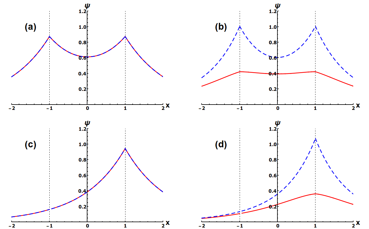
Figure 1: Possible solutions of (24) plotted as the wavefunctions $\psi$ (red, solid) as well as $\phi$ (blue, dashed) corresponding to the cases when: (a) both symmetries are conserved, (b) the symmetry between both cores is broken, (c) only intra-core-symmetry is broken and (d) both symmetries are broken. These wavefunctions are numerical solutions of (24) for $\mu=-0.9$ and $\kappa=0.5$

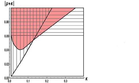
Figure 2: The phase diagram, in the $\left(\kappa,\left|\mu+\kappa\right|\right)$ plane, illustrating regions where solutions of different types exist. Solutions with unbroken symmetry exist everywhere. Above horizontal line $\mu_{+}=0.06$, in the horizontally shaded region, one additionally finds solutions with broken intra-channel symmetry. In the vertically shaded region, there appear solutions with broken symmetry between the channels ($u$ and $v$). In the pink region, there exists solutions both symmetries simultaneously broken . Note that there is a small triangular region where only fully symmetric solutions and ones with both symmetries broken can be found (the unshaded pink area).

The solutions of the system of nonlinear equations (6), in the form defined by Eqs. (22) and (24), are the main analytical result of the present work. They are analyzed through the rest of the paper in the context of the twofold spontaneous symmetry breaking in the system’s ground state, between the areas of $x>0$ and $x<0$, and between components $u$ and $v$ . We show that, depending on parameters of the system, $\kappa$ and $\mu$, solutions of different kinds (co)exist, viz., completely symmetric ones, or solutions which break the symmetry between the channels, or break the parity (symmetry with respect to the origin) in each channel, or, finally, solutions breaking both symmetries (cf. functions presented in Fig. 1).

Coupled algebraic equations (24), to which the use of the ideal delta-functions makes it possible to reduce the solution of Eq. (6), cannot be solved analytically (unlike the explicitly solution which is possible in the single-component model Dong ). It is, nevertheless, relatively easy to find all physically relevant solutions of Eq. (24) numerically, and thus classify all the solutions according to their symmetry.

In general, there are $3^{4}=81$ solutions, but many of them are highly degenerate. We summarize the results in the schematic form in Fig. (2), in the parameter plane of linear coupling $\kappa$ and shifted chemical potential $|\mu+\kappa|$. Ground-state solutions with both symmetries broken were found only in the region painted in pink. Next, as shown below, only above the horizontal line of $|\mu+\kappa|=0.06$ one can find stationary solutions with the broken $x\leftrightarrow-x$ symmetry, and only above the slanted nearly straight line, originating from the origin, there exist solutions with the symmetry broken between components $u$ and $v$. Below we derive conditions that predict these borders, and illustrate specific cases for selected values of $\kappa$, realizing scenarios of the spontaneous breaking of both symmetries. Note, however, that in Fig. (2) there is also a region where only the solutions with preserving full symmetry or with both symmetries broken exist. In this region there are no solutions with only one symmetry broken.

Figure 3: Stationary states for a fixed value of the inter-core coupling constant, $\kappa=0.05$. Panels (a) and (b): the energy and norm of the fully symmetric states (black), ones with broken inter-core symmetry (orange), and states with broken $x\leftrightarrow-x$ symmetry in each channel (blue), as functions of the chemical potential. The inset in (a) displays details of the emergence of the asymmetric states from the symmetric one. Panel (c) displays the corresponding symmetry-breaking bifurcations by means of asymmetry parameters $\Theta_{1}$ and $\Theta_{2}$ (the orange and blue curves, respectively, see Eqs. (25) and (26), plotted versus the total norm.

In the following we fixed the value of $\kappa$, and by varying the chemical potential, we sampled solutions along vertical lines in Fig. 2. Our results are outlined in Figs. 3 and 4, for $\kappa=0.05$ and $\kappa=0.2$, respectively. In order to describe these figures we introduce asymmetry parameters $\Theta_{1}$ and $\Theta_{2}$. The asymmetry between the $u$ and $v$ components is characterized by parameter

$$\Theta_{1}=\frac{\int_{-\infty}^{+\infty}\left[|u^{2}(x)|-|v^{2}(x)|\right]dx}{\int_{-\infty}^{+\infty}\left[|u^{2}(x)|+|v^{2}(x)|\right]dx},$$ (25)

and asymmetry with respect to the parity transformation, $x\longrightarrow-x$, is quantified by

$$\Theta_{2}=\frac{\int_{-\infty}^{0}\left[|u^{2}(x)|+|v^{2}(x)|\right]dx-\int_{0}^{+\infty}\left[|u^{2}(x)|+|v^{2}(x)|\right]dx}{\int_{-\infty}^{+\infty}\left[u^{2}(x)+v^{2}(x)\right]dx}.$$ (26)

In Fig. (3), we vary $\mu$ to the point of crossing the slanted line in Fig. 2, at $\mu\approx-0.062$. This is the border line above which (unstable) states featuring the asymmetry between the cores appear, only symmetric and antisymmetric states existing below this border. These asymmetric solutions are shown by the dashed orange line. Upon further decreasing the chemical potential we eventually enter the region where new solutions appear, with parity symmetries broken, which are represented by the blue dashed line in Fig. 3. Panels (a) and (b) show the norm and energy of these states as functions of the chemical potential, while panel (c) shows the asymmetry parameters $\Theta_{1}$ and $\Theta_{2}$ (see Eqs. (25) and (26) as functions of the norm, revealing that both symmetry-breaking bifurcations are of the subcritical bifurcations  type.

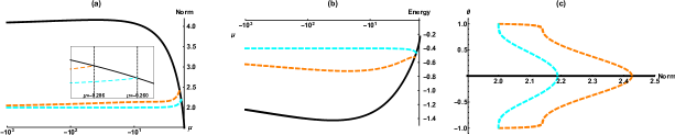
Figure 4: Stationary states for fixed value of $\kappa=0.2$. Panels (a) and (b): energy and norm of the symmetric state (black), states with broken inter-core symmetry (orange), and states with broken $x\leftrightarrow-x$ symmetry in each channel (blue), vs. the chemical potential. The inset in (a) displays details of the emergence of the asymmetric states from the symmetric one. In panel (c), the corresponding symmetry-breaking bifurcations are shown by means of asymmetry parameters $\Theta_{1}$ and $\Theta_{2}$ (the orange and blue curves, respectively, see Eqs. (25) and (26), plotted versus the total norm.

In Fig. (4) the black curve of symmetric states traverses the horizontal line into the region where (unstable) solutions, asymmetric with respect to $x\leftrightarrow-x$, appear (the blue dashed lines), and the second symmetry is broken at $\mu=-0.286$, to produce the states with inter-core symmetry broken (orange lines). Again, both bifurcations have the subcritical character.

In the next two sections we investigate asymmetry solutions, to identify the respective bifurcations. First we restrict the analysis to the class of solutions that remain symmetric (or antisymmetric) with respect to $x\leftrightarrow-x$ in each core. Within this class, we consider the possibility of the symmetry breaking between the cores. Next, we summarize findings obtained in previous works for the single-component model, which corresponds to the setting which maintains the symmetry or antisymmetry between the cores ($u=\pm v$). In the case of the spatial symmetry breaking ($x\leftrightarrow-x$), the model predicts a subcritical type of the spontaneous symmetry breaking. In that context, it is interesting to investigate to what extend the structure of the model affects the transition to the asymmetric states. To this end, we consider various forms of the nonlinearity modulation patterns, including an additional linear potential. Before addressing the model with the double delta function, as defined by Eq. (4), we first consider the profile of $g(x)$ with a single delta function.

III Solutions preserving the spatial symmetry in the cores

III.1 The basic model

The first type of the symmetry breaking, which was not studied in previous works, occurs under the assumption that the wave function remains spatially symmetric (even) or antisymmetric (odd), with respect to $x\leftrightarrow-x$, in each core, while the wave functions in the two cores may become different, $u\neq v$. As concerns coefficients in expression (21) for the solutions, this type of the localized states is ensured by setting $A=B$ and $C=D$. To obtain fully symmetric states, we choose $C=D=0$; then, it is straightforward to obtain from Eq. 24 a previously known solution Dong ,

$$A=B=\pm\sqrt{\frac{\sqrt{\mu_{+}}}{1+e^{-2\sqrt{\mu_{+}}}}}.$$ (27)

Likewise, for antisymmetric states we assume $A=B=0$ to obtain

$$C=D=\pm\sqrt{\frac{\sqrt{\mu_{-}}}{1+e^{-2\sqrt{\mu_{-}}}}}$$ (28)

Searching for states asymmetric between the parallel-coupled cores, we assume that all coefficients $A=B$ and $C=D$ are different from zero. In this case, solutions of Eq. (24) are

$$A = B=\pm\sqrt{\frac{3\sqrt{\mu_{-}}\left(1+e^{-2\sqrt{\mu_{+}}}\right)-\sqrt{\mu_{+}}\left(1+e^{-2\sqrt{\mu_{-}}}\right)}{8\left(1+e^{-2\sqrt{\mu_{-}}}\right)\left(1+e^{-2\sqrt{\mu_{+}}}\right)}},$$

$$C = D=\pm\sqrt{\frac{3\sqrt{\mu_{+}}\left(1+e^{-2\sqrt{\mu_{-}}}\right)-\sqrt{\mu_{-}}\left(1+e^{-2\sqrt{\mu_{+}}}\right)}{8\left(1+e^{-2\sqrt{\mu_{-}}}\right)\left(1+e^{-2\sqrt{\mu_{+}}}\right)}}.$$ (29)

To find the symmetry-breaking bifurcation point, we inspect the second expression in Eq. 29, equating the numerator under the square root to zero. This leads to

$$3\sqrt{\frac{|\mu_{\mathrm{bif}}+\kappa|}{|\mu_{\mathrm{bif}}-\kappa|}}=\frac{1+e^{-2\sqrt{2|\mu_{\mathrm{bif}}+\kappa|}}}{1+e^{-2\sqrt{2|\mu_{\mathrm{bif}}-\kappa|}}},$$ (30)

which is the main result of this section. It corresponds to the almost straight slanted border line in Fig. (2). We stress that, in the present model, all states besides totally symmetric ones are unstable. In particular, the states that exist above the line defined by Eq. (30), which are asymmetric with respect to the two cores ($u\neq v$), are unstable. Actually, this is the property of this particular model. In Section 5 we introduce a two-dimensional model, in which broken-symmetry solutions are stable.

We supplement this section by the following subsection, revealing the type of the symmetry-breaking bifurcation that one may expect dealing with models consisting of two identical cores and various nonlinearity-modulation patterns or linear potentials.

III.2 Review of related models

We first consider the case of the simplified spatial modulation with

$$g\left(x\right)=-\delta\left(x\right),$$ (31)

representing one singularity instead of two. In this case, exact solution (21) is replaced by

$$u = \left\{\begin{array}[]{c}Ae^{\sqrt{\mu_{+}}x}+Ce^{\sqrt{\mu_{-}}x},~{}\mathrm{at}~{}~{}x<0,\\ Ae^{-\sqrt{\mu_{+}}x}+Ce^{-\sqrt{\mu_{-}}x},~{}\mathrm{at}~{}~{}x>0,\end{array}\right.$$ (34)

$$v = \left\{\begin{array}[]{c}Ae^{\sqrt{\mu_{+}}x}-Ce^{\sqrt{\mu_{-}}x},~{}\mathrm{at}~{}~{}x<0,\\ Ae^{-\sqrt{\mu_{+}}x}-Ce^{-\sqrt{\mu_{-}}x},~{}\mathrm{at}~{}~{}x>0.\end{array}\right.$$ (37)

The conditions for the derivative jump at $x=0$ are $\Delta\left(u^{\prime}\right)|_{x=0}=-2\left(u|_{x=0}\right)^{3}$ and $\Delta\left(v^{\prime}\right)|_{x=0}=-2\left(v|_{x=0}\right)^{3}$, cf. Eq. (23). This leads to the system of coupled cubic equations

$$\sqrt{\mu_{+}}A+\sqrt{\mu_{-}}C = \left(A+C\right)^{3},$$

$$\sqrt{\mu_{+}}A-\sqrt{\mu_{-}}C = \left(A-C\right)^{3},$$ (38)

cf. Eq. (24), which can be easily solved. For the asymmetric solution, with $A\neq 0$ and $C\neq 0$, the amplitudes are

$$A = \pm\frac{1}{2}\sqrt{\frac{3}{2}\sqrt{\mu_{-}}-\frac{1}{2}\sqrt{\mu_{+}}},$$

$$C = \pm\frac{1}{2}\sqrt{\frac{3}{2}\sqrt{\mu_{+}}-\frac{1}{2}\sqrt{\mu_{-}}}.$$ (39)

The symmetry-breaking bifurcation point is derived by setting $C=0$ in Eq. (39), which yields

$$\mu_{\mathrm{bif}}=-\frac{5}{4}\kappa.$$ (40)

Note that, when the inter-core coupling is negligible, i.e. $\kappa=0$, the asymmetric states have $\mu<0$, hence they exist everywhere in the trapped-mode regime. On the other hand, the symmetry breaking does not take place for $\kappa\rightarrow\infty$, the solution keeping the form of $u=v$.

Amplitudes of the symmetric and antisymmetric states ($u=v$ and $u=-v$) can be easily found too. In particular, amplitudes of the symmetric state amount to $A^{2}=\sqrt{\mu_{+}/2}$ and $C^{2}=\sqrt{\mu_{-}/2}$, and norm (2) of symmetric and antisymmetric states is $N_{\mathrm{symm}}=N_{\mathrm{antisymm}}=2$. The norm of the asymmetric state is

$$N_{\mathrm{asymm}}=-\frac{3\mu+\sqrt{\mu^{2}-\kappa^{2}}}{2\sqrt{\mu^{2}-\kappa^{2}}},$$ (41)

with limit value $N_{\mathrm{asymm}}(\mu\rightarrow-\infty)=1$. The norms of the symmetric and asymmetric modes are plotted, as functions of $\mu$, in Fig. 5(a).

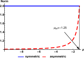
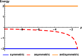
Figure 5: Norm (a) and energy (b) of the symmetric, antisymmetric and asymmetric states as a function of the chemical potential in the model with the nonlinearity modulation in the form of the single delta-function, as defined by Eq. (31). Solid and dashed lines denote stable and unstable states, respectively.

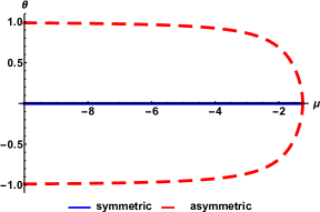
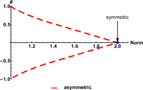
Figure 6: Asymmetry parameter $\Theta$, defined as per Eq. (43), as a function of the chemical potential (a) and total norm (b). Solid and dashed lines correspond to stable and unstable states, respectively.

The value of the energy (Hamiltonian), defined in Eq. (3), can also be calculated for all the states under the consideration, a general expression being

$$E=\sqrt{\mu_{+}}|A|^{2}+\sqrt{\mu_{-}}|C|^{2}-|A|^{4}-A^{2}\left(C^{\ast}\right)^{2}\\ -4|A|^{2}|C|^{2}-\left(A^{\ast}\right)^{2}C^{2}-|C|^{4}-\frac{\kappa|A|^{2}}{\sqrt{\mu_{+}}}+\frac{\kappa|C|^{2}}{\sqrt{\mu_{-}}}.$$

In the special cases of the symmetric, antisymmetric and asymmetric states the corresponding energies are $E_{\mathrm{symm}}=-\kappa$ and $E_{\mathrm{antisymm}}=\kappa$, and

$$E_{\mathrm{asymm}}=-\frac{3}{8}\kappa\left[\sqrt{\frac{\mu_{-}}{\mu_{+}}}-\sqrt{\frac{\mu_{+}}{\mu_{-}}}\right].$$ (42)

At the bifurcation point (see Fig. 5(b)), $\mu=-\left(5/4\right)\kappa$, expression (42) coincides with $E_{\mathrm{symm}}=-\kappa$.

Finally, asymmetry coefficient (25), which measures the norm imbalance between the cores, is calculated for solution (39) as

$$\Theta=\frac{4\sqrt{5\sqrt{\mu^{2}-\kappa^{2}}+3\mu}\cdot\sqrt{\mu^{2}-\kappa^{2}}}{\left(-3\mu-\sqrt{\mu^{2}-\kappa^{2}}\right)\left(\sqrt{-2(\mu+\kappa)}+\sqrt{-2(\mu-\kappa)}\right)}.$$ (43)

It is plotted versus the chemical potential and norm in Fig. 6. Note that $\Theta\rightarrow 1$ in the limit of ${\mu\rightarrow-\infty}.$ All the asymmetric states are unstable, in the model based on the single-delta modulation format (31).

Numerical investigation was also performed for similar models with the single delta function replaced by a finite-width Gaussian. In this case, the symmetry-breaking bifurcation keeps the subcritical form even in the case of a broad Gaussian, cf. Fig. 6(b). This finding is in agreement with the fact that, in various models of dual-core couplers with the uniform self-focusing nonlinearity, symmetry-breaking bifurcations for solitons are subcritical too Laval -Skinner , bifurcations ; Hung . Additionally, we have investigated the model of the coupled cores with the uniform self-focusing nonlinearity, combined with a local defect represented by a linear-potential well (not shown here in detail). In this case, we have found the subcritical transition in shallow wells, regardless of their width, which carry over into a supercritical transition when the well’s depth exceeds a certain critical value.

IV The case of the symmetry maintained between the cores

Here we present a short summary of results obtained when we impose the condition of the symmetry between the cores, i.e. $u=\pm v$, comparing this case to the study presented in Ref. Dong , where the spontaneous symmetry breaking in was due to the action of the nonlinear potential with two symmetric minima. When the respective modulation pattern was taken as per Eq. (4), a fully analytical solution was obtained for symmetric, antisymmetric, and asymmetric states, the respective symmetry-breaking bifurcation was ultimately subcritical, with the branches of asymmetric localized states never turning in the forward direction.

In terms of Eqs. (24), the cases of $u=v$ and $u=-v$ correspond, respectively, to setting $C=D=0$ and $A=B=0$. In the former (symmetric) case the remaining equations for amplitudes $A$ and $B$ rare

$$\sqrt{\mu_{+}}e^{2\sqrt{\mu_{+}}}\left(e^{2\sqrt{\mu_{+}}}B-A\right) = \left(e^{4\sqrt{\mu_{+}}}-1\right)B^{3},$$

$$\sqrt{\mu_{+}}e^{2\sqrt{\mu_{+}}}\left(e^{2\sqrt{\mu_{+}}}A-B\right) = \left(e^{4\sqrt{\mu_{+}}}-1\right)A^{3}.$$ (44)

To treat the antisymmetric, one may replace $A\rightarrow C$, $B\rightarrow D$ and $\mu_{+}\rightarrow\mu_{-}$. The respective solutions are

$$A=B\equiv A_{\mathrm{sym}}=\pm\sqrt{\frac{\sqrt{\mu_{+}}}{1+e^{-2\sqrt{\mu_{+}}}}},$$ (45)

and an antisymmetric form (i.e. antisymmetry in each channel)

$$A=-B\equiv A_{\mathrm{antisymm}}=\pm\sqrt{\frac{\sqrt{\mu_{+}}}{1-e^{-2\sqrt{\mu_{+}}}}}.$$ (46)

The norm of these solutions is

$$N_{\mathrm{symm},\mathrm{antisymm}}=\frac{1}{1\pm e^{-2\sqrt{\mu_{+}}}}+\frac{1-e^{-4\sqrt{\mu_{+}}}\pm 4\sqrt{\mu_{+}}e^{-2\sqrt{\mu_{+}/2}}}{\left(1\pm e^{-2\sqrt{\mu_{+}/2}}\right)},$$ (47)

where $+$ and $-$ correspond to the symmetric and antisymmetric ones, respectively. Both solutions are characterized by the same asymptotic limit, $N_{\mu\rightarrow-\infty}\rightarrow 2$. The chemical potential at the bifurcation point is evaluated, for the symmetric solution, (in agreement with Dong ) as

$$\tilde{\mu}_{\mathrm{bif}}=-\left(\ln 2\right)^{2}/8\approx 0.06,$$ (48)

while the antisymmetric one undergoes no bifurcation. Likewise, the amplitudes for asymmetric states can be found analytically,

$$\left\{A,B\right\}_{\mathrm{asymm}}=\frac{\sqrt[4]{\mu_{+}/2}\left(\sqrt{1+2e^{-2\sqrt{\mu_{+}}}}\pm\sqrt{1-2e^{-2\sqrt{\mu_{+}}}}\right)}{2^{3/4}\sqrt{1-e^{-4\sqrt{\mu_{+}}}}},$$ (49)

and the bifurcation point derived from this solution is identical to one given by Eq. (48).

In the case when symmetry $u=\pm v$ is imposed, we can compare our results with the more realistic model of with the Gaussian modulation format Dong ,

$$g\left(x\right)=\frac{-1}{a\sqrt{\pi}}\left[\exp\left(-\frac{\left(x+1\right)^{2}}{a^{2}}\right)+\exp\left(-\frac{\left(x-1\right)^{2}}{a^{2}}\right)\right],$$ (50)

where the modulated nonlinearity coefficient is subject to the normalization condition $\int_{-\infty}^{+\infty}g\left(x\right)dx=2.$ It is found that, at a certain value of width $a$ of the Gaussian pattern (50), a transition to the supercritical type of the symmetry-breaking bifurcation takes place. On the other hand, if we consider systems with uniform self-focusing nonlinearity in the presence of a linear potential representing a double potential well DWP1 ; DWP2 ; Marek , spontaneous symmetry breaking occurs too, but it always has the supercritical character.

V Double symmetry breaking in two dimensions

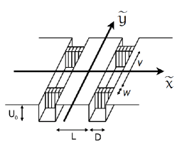
Figure 7: The combination of the linear-potential double-trough trapping acting along the $x$ direction, and the localized nonlinearity pattern shown by the striped structure. We address double symmetry breaking of two-dimensional solitons in this setting.

In the previous sections we considered solutions of coupled one-dimensional systems with the nonlinearity concentrated at two narrow spots, finding stationary states with one of the symmetries broken (ether between the parallel-coupled cores, or between the two nonlinear spots in the cores), or even the situation when both underlying symmetries are broken in the stationary state. In most cases, however, and in all cases when the nonlinearity modulations is based on the pair of delta-functions (Eq. (4)), states with broken symmetry were unstable. One can argue that the model with the ideal delta-functions is degenerate, which is reflected in the character of the stationary states. In this section, we do not consider bifurcations and spontaneous symmetry breaking for settings with the Gaussian nonlinearity-modulation profiles, replacing the two delta-functions. Instead of that, in this section we focus on a two-dimensional model with localized nonlinearity, showing that in this case states with broken symmetries may be stable. The setting that we address is based on the following GPE,

$$i\frac{\partial\psi}{\partial t}=-\frac{1}{2}\left(\frac{\partial^{2}\psi}{\partial x^{2}}+\frac{\partial^{2}\psi}{\partial y^{2}}\right)+g\left(x,y\right)|\psi|^{2}\psi+U(x)\psi.$$ (51)

As displayed in Fig. 7, potential $U(x)$ creates the double-well (double-trough) trapping potential acting in the $x$ direction, while nonlinearity coefficient $g\left(x,y\right)$ is concentrated at four localized spots (striped in the figure). This model may be considered as a two-dimensional extension of the one-dimensional model introduced above.

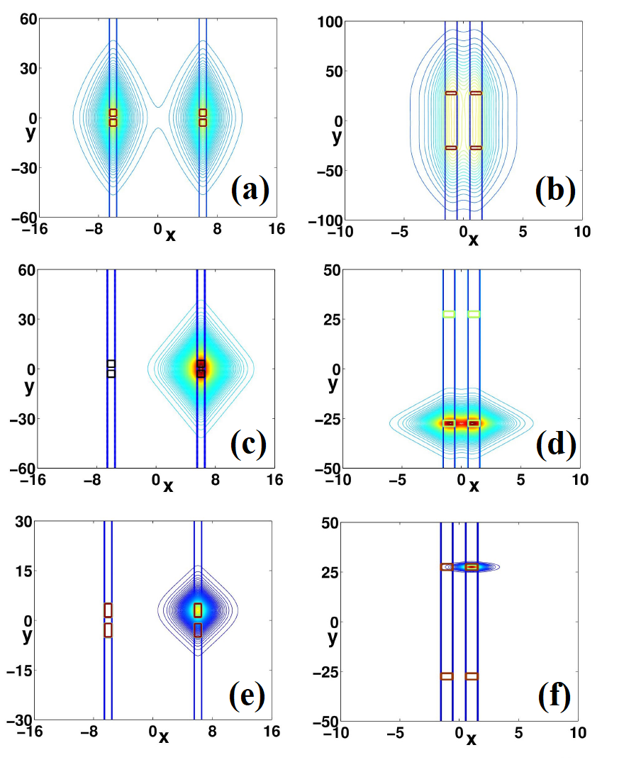
Figure 8: Contour plots of the local density illustrating stable two-dimensional self-trapped states. Panels (a) and (b): fully symmetric ones. (c) and (d): States with broken symmetry between the two cores, and between the two nonlinear spots, respectively. States featuring the breaking of both symmetries are displayed in panels (e) and (f).

We used the imaginary-time method IT to find ground states of the system. Their stability was then confirmed by simulating the real time evolution (using the split-step Fourier method). We have observed four types of stable solitons, which are shown in Fig. 8. The figure confirms that, depending on the value of the norm, stable states with all possible combinations of the asymmetry can be produced. A general conclusion, suggested by the systematic simulations, is that, in the model with weaker coupling between the cores, it is easier to find stable states with the broken symmetry between the cores. With the increase of the norm, states with both symmetries broken are found too. On the other hand, the symmetry between the nonlinearity-concentration spots in both cores in broken first in the setting with the nonlinearity spots set closer to each other. In particular, values of parameters in Fig. 8 are:
in Figs. 8 (a), (c) and (e), $L=11$, $D=1$, $W=4$, $V=2$, and the norm in the increasing order, $N=0.6$, $N=1.5$, and $N=2.5$, respectively. Similarly, in Fig. 8 (b), (d) and (f), the parameters are $L=1$, $D=1$, $W=3$, $V=52$, and norms are, respectively, $N=1$, $4$, and $5.1$. The depth of linear potential $U_{0}$ and the (constant) value of the nonlinear coupling can be rescaled. The strength of the interaction is now contained in the norm of the wavefunction.

In the real-time simulations, we added small perturbations to check if the input states maintain their initial shapes after long evolution. All of the above states still survive, at least, up to $t=1000$.

Our two-dimensional model surely deserves further investigation, including the identification of bifurcation diagrams, regions of stability of various types of solutions, and studies of dynamical behavior, including collisions between solitons. Detailed results addressing these issues will be reported elsewhere.

VI Conclusion

The objective of this work is to investigate the phenomenology of spontaneous symmetry breaking in the class of dual-core systems featuring the additional spatial symmetry in each core, induced by the nonlinearity-modulation pattern in the form of two tightly localized spots, which may be approximated, in some cases, by ideal delta-functions. In this case, solutions for stationary one-dimensional states can be obtained in the implicit analytical form, represented by coupled cubic equations for constituent amplitudes. The analysis makes it possible to construct modes with broken inter-core and intra-core symmetries, as well as ones featuring the double breaking of both symmetries. While all such asymmetric modes turn out to be unstable, the consideration of the most interesting two-dimensional version of the system, with a small transverse thickness of each core, and a small finite size of the nonlinearity-localization spots, reveals stable asymmetric states of all the types, including ones realizing the double symmetry breaking.

As an extension of the analysis, it may be interesting to construct stationary patterns in which the complex wave function, peaked at the nonlinearity-localization spots, features a phase structure which corresponds to trapped vorticity, following the pattern of Ref. Kevrekidis . The existence and stability of such vortex modes, with unbroken or broken symmetries, is a challenging issue.

- (1) W. P. Huang, “Coupled-mode theory for optical waveguides: an overview”, J. Opt. Soc. Am. A 1994, 11, 963-983.
- (2) M. J. F. Digonnet and H. J. Shaw, “Analysis of a tunable single-mode optical fiber coupler”, IEEE J. Quant. Electr. 1982, 18, 746-754.
- (3) S. Trillo, S. Wabnitz, E. M. Wright, and G. I. Stegeman, “Soliton switching in fiber nonlinear directional couplers”, Opt. Lett. 1988, 13, 672-674.
- (4) H. Harsoyono, R. E. Siregar, and M. O. Tjia, “A study of nonlinear coupling between two identical planar waveguides”, J. Nonlin. Optical Phys. & Materials, 2001, 10, 233-247.
- (5) K. E. Strecker, G. B. Partridge, A. G. Truscott, and R. G. Hulet, “Bright matter wave solitons in Bose-Einstein condensates”, New J. Phys. 2003, 5, 73.1.
- (6) A. Gubeskys and B. A. Malomed, “Symmetric and asymmetric solitons in linearly coupled Bose-Einstein condensates trapped in optical lattices”, Phys. Rev. A 2007, 75, 063602.
- (7) L. Salasnich, B. A. Malomed, and F. Toigo, “Competition between the symmetry breaking and onset of collapse in weakly coupled atomic condensates”, Phys. Rev. A 2010, 81, 045603.
- (8) M. Matuszewski, B. A. Malomed, and M. Trippenbach, “Spontaneous symmetry breaking of solitons trapped in a double-channel potential”, Phys. Rev. A 2007, 75, 063621.
- (9) L. Pitaevskii and S. Stringari, Bose-Einstein Condensation, 2003. Clarendon: Oxford, UK.
- (10) S. M. Jensen, “The nonlinear coherent coupler”, IEEE Journal of Quantum Electr. 1982, 18, 1580-1583.
- (11) A. A. Maier, “Optical transistors and bistable devices utilizing nonlinear transmission of light in systems with unidirectional coupled waves”, Sov. J. Quant. Electron. 1982, 12, 1490-1494.
- (12) S. R. Friberg, Y. Silberberg, M. K. Oliver, M. J. Andrejco, M. A. Saifi, and P. W. Smith, Ultrafast all-optical switching in dual-core fiber nonlinear coupler, Appl. Phys. Lett. 51, 1135-1137 (1987).
- (13) S. R. Friberg, A. M. Weiner, Y. Silberberg, B. G. Sfez, and P. S. Smith, “Femtosecond switching in dual-core-fiber nonlinear coupler”, Opt. Lett. 1988, 13, 904-906.
- (14) D. R. Heatley, E. M. Wright, and G. I. Stegeman, “Soliton coupler”, Appl. Phys. Lett. 1988, 53, 172-174.
- (15) W. Królikowski and Y. S. Kivshar, “Soliton-based optical switching in waveguide arrays”, J. Opt. Soc. Am. B 1996, 13, 876-887.
- (16) S. C. Tsang, K. S. Chiang, and K. W. Chow, “Soliton interaction in a two-core optical fiber”, Opt. Commun. 2004, 229, 431-439.
- (17) I. M. Uzunov, R. Muschall, M. Gölles, Yu. S. Kivshar, B. A. Malomed, and F. Lederer, “Pulse switching in nonlinear fiber directional couplers”, Phys. Rev. E 1995, 51, 2527-2537.
- (18) F. Lederer, G. I. Stegeman, D. N. Christodoulides, G. Assanto, M. Segev, and Y. Silberberg, “Discrete solitons in optics”, Phys. Rep. 2008, 463, 1-126.
- (19) A. W. Snyder, D. J. Mitchell, L. Poladian, D. R. Rowland, and Y. Chen, “Physics of nonlinear fiber couplers”, J. Opt. Soc. Am. B 1991, 8, 2102-2112.
- (20) E. M. Wright, G. I. Stegeman, S. Wabnitz, “Solitary-wave decay and symmetry-breaking instabilities in two-mode fibers”, Phys. Rev. A 1989, 40, 4455 (1989).
- (21) C. Paré and M. Florjańczyk, “Approximate model of soliton dynamics in all-optical fibers”, Phys. Rev. A 1990, 41, 6287-6295.
- (22) A. I. Maimistov, “Propagation of a light pulse in nonlinear tunnel-coupled optical waveguides”, Kvantovaya Elektron. (Moscow) 1991, 18, 758-761 [Sov. J. Quant. Electr. 1991, 21, 687-690].
- (23) P. L. Chu, B. A. Malomed, and G. D. Peng, “Soliton switching and propagation in nonlinear fiber couplers: analytical results”, J. Opt. Soc. Am. B 1993, 10, 1379-1385.
- (24) N. Akhmediev and A. Ankiewicz, “Novel soliton states and bifurcation phenomena in nonlinear fiber couplers”, Phys. Rev. Lett. 1993, 70, 2395-2398
- (25) J. M. Soto-Crespo and N. Akhmediev, “Stability of the soliton states in a nonlinear fiber coupler”, Phys. Rev. E 1993, 48, 4710-4715.
- (26) B. A. Malomed, I. M. Skinner, P. L. Chu, and G. D. Peng, “Symmetric and asymmetric solitons in twin-core nonlinear optical fibers”, Phys. Rev. E 1996, 53, 4084-4091.
- (27) S. Trillo, G. Stegeman, E. Wright, and S. Wabnitz, “Parametric amplification and modulational instabilities in dispersive nonlinear directional couplers with relaxing nonlinearity”, J. Opt. Soc. Am. B 1989, 6, 889-900.
- (28) R. S. Tasgal and B. A. Malomed, “Modulational instabilities in the dual-core nonlinear optical fiber”, Physica Scripta 1999, 60, 418-422.
- (29) K. S. Chiang, “Intermodal dispersion in two-core optical fibers”, Opt. Lett. 1995, 20, 997-999.
- (30) M. Romagnoli, S. Trillo and S. Wabnitz, “Soliton switching in nonlinear couplers”, Opt. Quantum Electron. 1992, 24, S1237-S1267.
- (31) B. A. Malomed, “Variational methods in fiber optics and related fields”, Progr. Optics 2002, 43, 71-193.
- (32) B. A. Malomed, “Solitons and nonlinear dynamics in dual-core optical fibers”, in Handbook of Optical Fibers 2018 (G.-D. Peng, Editor: Springer)
- (33) G. Iooss and D. D. Joseph, Elementary Stability and Bifurcation Theory 1990 (Springer: Berlin).
- (34) J. Hukriede, D. Runde, and D. Kip, “Fabrication and application of holographic Bragg gratings in lithium niobate channel waveguides,” J. Phys. D 2003, 36, R1.
- (35) L. W. Clark, L.-C. Ha, C.-Y. Xu, and C. Chin, Quantum dynamics with spatiotemporal control of interactions in a stable Bose-Einstein condensate”, Phys. Rev. Lett. 2015, 115, 155301.
- (36) B. A. Malomed, editor, Spontaneous Symmetry Breaking, Self-Trapping, and Josephson Oscillations 2013 (Springer-Verlag: Berlin and Heildelberg), ISBN: 978-3-642-21206-2
- (37) Y. Li, B. A. Malomed, M. Feng, and J. Zhou, Double symmetry breaking of solitons in one-dimensional virtual photonic crystals, Phys. Rev. A 2011, 83, 053832.
- (38) T. Mayteevarunyoo, B. A. Malomed, and G. Dong, ”Spontaneous symmetry breaking in a nonlinear double-well structure”, Phys. Rev. A 2008, 78, 053601.
- (39) L. Salasnich, A. Parola, and L. Reatto, “Effective wave equations for the dynamics of cigar-shaped and disk-shaped Bose condensates”, Phys. Rev. A 2002, 65, 043614.
- (40) A. Muñoz Mateo and V. Delgado, “Effective mean-field equations for cigar-shaped and disk-shaped Bose-Einstein condensates”, Phys. Rev. A 2008, 77, 013617.
- (41) H. Sakaguchi and B. A. Malomed, ”Symmetry breaking of solitons in two-component Gross-Pitaevskii equations”, Phys. Rev. E 2011 83, 036608.
- (42) A. Acus, B. A. Malomed, and Y. Shnir, ”Spontaneous symmetry breaking of binary fields in a nonlinear double-well structure”, Physica D 2012, 241, 9872.
- (43) X.-F. Zhou, S.-L. Zhang, Z.-W. Zhou, B. A. Malomed, and H. Pu, Bose-Einstein condensation on a ring-shaped trap with nonlinear double-well potential, Phys. Rev. A 2012, 85, 023603.
- (44) N. V. Hung, P. Zin, M. Trippenbach, and B. A. Malomed, ”Two-dimensional solitons in media with stripe-shaped nonlinearity modulation” Phys. Rev. E 2010, 82, 046602.
- (45) G. J. Milburn, J. Corney, E. M. Wright, and D. F. Walls, “Quantum dynamics of an atomic Bose-Einstein condensate in a double-well potential”, Phys. Rev. A 1997, 55, 4318-4324.
- (46) A. Smerzi, S. Fantoni, S. Giovanazzi, and S. R. Shenoy, “Quantum coherent atomic tunneling between two trapped Bose-Einstein condensates”, Phys. Rev. Lett.1997, 79, 4950-4953.
- (47) M. L. Chiofalo, S. Succi, and M. P. Tosi, “Ground state of trapped interacting Bose-Einstein condensates by an explicit imaginary-time algorithm”, Phys. Rev. E 2000, 62, 7438-7444.
- (48) B. A. Malomed and P. G. Kevrekidis, “Discrete vortex solitons”, Phys. Rev. E 2001, 64, 026601.