Force-dependent diffusion coefficient of molecular Brownian ratchets

Abstract

We study the mean velocity and diffusion constant in three related models of molecular Brownian ratchets. Brownian ratchets can be used to describe translocation of biopolymers like DNA through nanopores in cells in the presence of chaperones on the trans side of the pore. Chaperones can bind to the polymer and prevent it from sliding back through the pore. First, we study a simple model that describes the translocation in terms of an asymmetric random walk. It serves as an introductory example but already captures the main features of a Brownian ratchet. We then provide an analytical expression for the diffusion constant in the classical model of a translocation ratchet that was first proposed by Peskin et al. . This model is based on the assumption that the binding and unbinding of the chaperones are much faster than the diffusion of the DNA strand. To remedy this shortcoming, we propose a modified model that is also applicable if the (un)binding rates are finite. We calculate the force-dependent mean velocity and diffusivity for this model and compare the results to the original one. Our analysis shows that for large pulling forces the predictions of both models can differ strongly even if the (un)binding rates are large in comparison to the diffusion timescale but still finite. Furthermore, implications of the thermodynamic uncertainty relation on the efficiency of Brownian ratchets are discussed.

I Introduction

Translocation of polymers through nanopores lies at the heart of many processes in biology. How exactly do polymers like single stranded DNA or a RNA chain pass through protein channels embedded in the membranes of the cell nucleus or the cell proper? This question is of interest both in biology and in soft matter physics simon_what_1992 ; zandi_what_2003 ; lim_mechanical_2006 ; chen_ins_2005 ; palyulin_polymer_2014 ; neupert_perspective_2015 ; knyazev_driving_2018 .

There are several different mechanisms that have been identified to help sliding nanoscopic chains through pores in an environment with thermal fluctuations. If the chain is charged, an electric field in the vicinity of the pore can pull the chain from the cis side to the trans side. Incidentally, measuring certain ionic currents that flow through the pore if the pore is clogged by a monomer can be used to identify that monomer. Artificially designed nanopores could therefore make it possible to sequence DNA as it passes through the pore, potentially outperforming other methods bezrukov_counting_1994 ; kasianowicz_characterization_1996 ; fyta_translocation_2011 .

There are also entropic forces at play in the translocation process since the possible configurations of the chain are restricted by the pore. Flexible polymer chains can, for example, retract from the pore after they have already partially translocated if the translocated segment straightens and enters a hairpinlike state fyta_hydrodynamic_2008 .

Yet a different mechanism that aids the translocation, which is the main interest of this paper, is provided by the binding of certain molecules to the chain on the trans side of the pore. In the context of protein translocation this role can be played by chaperone molecules, which are also important in the context of protein folding and can bind to the chain. Since chaperones are too large to pass through the pore, the movement of the chain gets biases towards the side with the higher concentration of chaperones. Translocation ratchets have been discussed in the context of various different translocation processes in biological systems hepp_bacterial_2017 ; craig_hsp70_2018 . Recent experiments showed that the uptake of DNA molecules by Neiseria gonorrhoeae bacteria hepp_kinetics_2016 can be described by a rather simple translocation ratchet model peskin_cellular_1993 . In this case ComE proteins in the periplasm can bind to the DNA chain and act in the same way as chaperones do in the case of protein translocation by preventing the strand from sliding out if they are bound.

Usually theoretical models predict only the mean velocity or the mean translocation time. It can, however, also be of interest to compare predictions of the diffusion constant, i. e. , the rate at which the variance of the traveled distance increases, from Brownian ratchet models with the experimental findings. Apart from studies like krapivsky_fluctuations_2010 predictions for the diffusion coefficient are sparse. For this reason, experimental data can only be compared to predictions of the mean velocity. Thereby, a significant part of information contained in probability distributions gained in experiments does not enter into fits of the model. The present paper aims to close this gap.

Considering the diffusion constant can also be of theoretical interest as recent developments regarding the thermodynamic uncertainty relation barato_thermodynamic_2015 ; gingrich_dissipation_2016 ; pietzonka_finite-time_2017a ; horowitz_proof_2017a have shown. This relation shows that high precision, i. e. , small fluctuations of quantities like performed work or traveled distance comes at the cost of a high dissipation rate. Since the uncertainty relation requires only a few assumptions, which are generically valid for processes at fixed temperature, it implicates a quite general relation between diffusion coefficient and mean velocity also for biological processes like translocation.

Covering the translocation process in its full complexity requires the use of involved numerical simulations. In the case of protein translocation with Hsp70, for example, chaperones models have been proposed that include forces applied by the chaperones to the strand, actively pulling it in delosrios_hsp70_2006 . We will, however, focus on the ratcheting mechanism that is caused by the binding of chaperones to the chain. Established models usually assume that the parts of the strand on both sides are in chemical equilibrium with their respective environments, which allows for the identification of a free energy associated with the position of the strand ambjornsson_chaperone-assisted_2004 ; ambjornsson_directed_2005 ; abdolvahab_analytical_2008 ; metzler_polymer_2010 ; abdolvahab_sequence_2011 ; abdolvahab_chaperone-driven_2017 . In contrast, we use a more detailed description in the spirit of the classical model of a translocation ratchet introduced by Peskin et al. peskin_cellular_1993 . The basic concept of our models is that the movement of the DNA strand would be governed by a process without directional preference if it were in equilibrium. However, on the trans side of the pore molecules bind to equidistant binding sites on the strand with rate $w_{\mathrm{on}}$ and unbind with rate $w_{\mathrm{off}}$. An occupied binding site can not pass through the pore. As a result the movement of the DNA is biased and can be used to perform work against a force. We assume that the strand is stiff. Effects of bending of the chain are investigated, e. g. , in yu_polymer_2014a ; adhikari_translocation_2015 ; suhonen_chaperone-assisted_2016 ; mondal_ratchet_2016 ; emamyari_polymer_2017 . Furthermore, we neglect the finite length of the strand and assume that the movement can go on in both directions indefinitely.

The paper is organized as follows. In Sec. II, we introduce a simple model for rectification based on an asymmetric random walk with an alternating set of rates. Although simple, the model shows two distinct features that we encounter also in more involved models. The strand is drawn in, when it is not pulled outwards by an external force. If it is, however, pulled strongly, the mean velocity reaches a finite limit. The classical model for rectified Brownian motion that was introduced in peskin_cellular_1993 is briefly recapitulated in Sec. III. In addition to the mean velocity, which was already calculated in the original work, we provide an analytical expression for the diffusion coefficient for this model. The key assumption that lets us treat the classical model analytically is the time-scale separation between the diffusion process of the strand and the binding process of the molecules that block transitions through the pore. A model that drops this assumption is studied numerically in Sec. IV. As a consequence of the thermodynamic uncertainty relation, which connects mean velocity, diffusion coefficient, and entropy production, the efficiency of the ratcheting process is bounded by a function that only depends on the measurable quantities $v$, $D$, and $f$. We study such thermodynamic implications provided by the uncertainty relation in Sec. IV.6. We summarize our findings in Sec. V.

II Simple Model

II.1 States and rates

The assumptions entering this model are that the probability of finding two consecutive empty binding sites is negligibly small and that it is possible to map the movement of the chain through the pore to a discrete jump process. Under these conditions the translocation process can be described as a two state Markov process (see Fig. 1). In state 1 all sites on the trans side are occupied and in state 2 the first site next to the pore is empty. There are two different ways to get from state 1 to 2. Either the whole strand moves further to the trans side by one position with rate $w_{1+}$, leaving the first pore empty, or the first chaperone unbinds with rate $w_{2-}$. Transitions in the opposite direction are also possible by the same mechanisms. The strand can jump backwards with rate $w_{1-}$ or the first binding site gets occupied with rate $w_{2+}$. Since this simple model is, by design, restricted to situations where it is unlikely to find two consecutive empty binding sites, the binding rate $w_{2+}$ should always be greater than the unbinding rate $w_{2-}$.

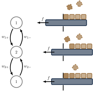
Figure 1: Schematic depiction of the alternating random walk model. The system can be in two different sates depending on whether the binding site in front of the pore is occupied or not. The state can either change by binding or unbinding of the chaperone on this site or by movement of the hole strand. These transition rates are assumed to obey a local detailed balance condition relating these rates to the binding energy and the pulling force.

Since the strand is pulled back by a force, the movement by one position in the forward direction is associated with the free energy difference $\Delta\mathcal{F}=-f$ and the local detailed balance condition reads

$$\frac{w_{1+}}{w_{1-}}=\mathrm{e}^{-f}\,.$$ (1)

Note that we set $k_{\mathrm{B}}T=1$ throughout and use the distance of two neighboring binding sites as the unit of length, rendering the force $f$ dimensionless. With this convention both the mean velocity and the diffusion constant have the unit of a frequency.

We also assume local detailed balance for the (un)binding transition relating the associated rates with the binding energy $\Delta E$ by the condition

$$\frac{w_{2+}}{w_{2-}}=\mathrm{e}^{\Delta E}.$$ (2)

Since our goal is to study the force dependence of mean velocity and diffusivity, we have to specify how each rate depends on the force applied to the system explicitly. Otherwise we would not be able to compare two configurations that only differ in the applied force. Equations (1) and (2), however, only fix the ratio of the rates in terms of the force and the binding energy. To fix each rate individually, additional assumptions on the force dependence have to be made. For the movement of the strand that is modeled by the rates $w_{1+}$ and $w_{1-}$ we assume that the pulling force affects the rates in a symmetrical manner, since the strand should not have a directional preference. This leads to the ansatz

$$w_{1+}=k\mathrm{e}^{-f/2}\quad\text{and}\quad w_{1-}=k\mathrm{e}^{f/2}\,,$$ (3)

where we introduce the rate constant $k$ that fixes the timescale of the movement of the strand. For the dynamics of the (un)binding process of the chaperone molecules there does not need to exist such a symmetry. We will, however, assume that the binding and unbinding rates do not depend on the force $f$. Therefore, we make the general ansatz

$$w_{2+}=w\quad\text{and}\quad w_{2-}=w\,\mathrm{e}^{-\Delta E}$$ (4)

introducing a positive constant $w$. It should be mentioned that the choice of putting the exponential term from Eq. (2) exclusively into the unbinding rate $w_{2-}$ has no physical meaning; it is done only because it simplifies some calculations later on. Any other choice of splitting the exponential term between the binding and unbinding rate can easily be accommodated by redefining $w$.

II.2 Mean velocity and diffusivity

In this section we calculate the mean velocity and diffusion coefficient for the minimal model introduced above. This is done by calculating the rescaled cumulant generating function (from here on simply called the generating function)

$$\alpha(\lambda)\equiv\lim_{t\rightarrow\infty}\frac{1}{t}\ln\left\langle\mathrm{e}^{\lambda\Delta x}\right\rangle\,,$$ (5)

where $\Delta x$ is the distance traveled by the strand during time $t$. The scaled cumulants $\mathcal{C}_{n}\equiv\lim_{t\rightarrow\infty}C_{n}/t$ are encoded in the generating function as its $n$th derivative at $\lambda=0$. The first two cumulants are the expectation value and the variance of the distribution of $\Delta x$, i. e. , $C_{1}=\langle\Delta x\rangle$ and $C_{2}=\langle(\Delta x-\langle\Delta x\rangle)^{2}\rangle$. It can be shown that the generating function is the largest eigenvalue of the so called tilted operator lebowitz_gallavotti-cohen-type_1999 .

The tilted operator associated with the total distance traveled by the strand is given by the matrix

$$\mathcal{L}(\lambda)=\left(\!\begin{array}[]{cc}-w_{1+}-w_{2-}&w_{1-}\mathrm{e}^{-\lambda/2}+w_{2+}\mathrm{e}^{\lambda/2}\\ w_{1+}\mathrm{e}^{\lambda/2}+w_{2-}\mathrm{e}^{-\lambda/2}&-w_{1-}-w_{2+}\end{array}\!\right).$$ (6)

It can be obtained from the master operator by multiplying every transition rate on the off-diagonals with an exponential term of the form $\mathrm{e}^{d\lambda}$, where $d$ is the increment of $\Delta x$ for a jump associated with the specific rate (see, e. g., koza_general_1999 for a derivation).

In this particular case the rescaled cumulant generating function can be obtained directly in closed form as the largest eigenvalue of $\mathcal{L}(\lambda)$. The mean velocity and variance of the position are the first and second derivatives of this function at $\lambda=0$. The calculations are straight forward but lead to rather lengthy expressions and are therefore not presented here. The result for the mean velocity is given by

$$v=\frac{w_{1+}w_{2+}-w_{1-}w_{2-}}{w_{1+}+w_{1-}+w_{2+}+w_{2-}}\,.$$ (7)

The expression for the diffusion coefficient can be put in the form

$$D=\frac{1}{2}\frac{w_{1+}w_{2+}+w_{1-}w_{2-}-2v^{2}}{w_{1+}+w_{1-}+w_{2+}+w_{2-}}\,.$$ (8)

II.3 Change of parametrization

The ansatz for the transitions rates introduces the two timescales $w$ and $k$ that parametrize the local detailed balance condition. These parameters are, however, not easy to determine experimentally. For this reason we express $w$ and $k$ in terms of more accessible quantities, namely, the velocity and diffusion coefficient without pulling force, which we denote by $v_{0}$ and $D_{0}$, respectively.

Replacing the timescales by velocity and diffusion without force eliminates the need to know the load sharing entering the binding rates as long as we assume that it does not depend on the force. For the jump rates of the strand, $w_{1+}$ and $w_{1-}$, the load sharing is assumed according to Eq. (3) with constant $k$.

Solving the equations $v(k,w,\Delta E,f=0)=v_{0}$ and $D(k,w,\Delta E,f=0)=D_{0}$ for $k$ and $w$ leads to a quadratic equation that yields the two sets of solutions

$$k^{{}^{\pm}} =\frac{v_{0}^{2}\left(\mathrm{e}^{\Delta E}-1\right)\pm v_{0}^{2}\sqrt{C(v_{0},D_{0},\Delta E)}}{2v_{0}\left(\mathrm{e}^{\Delta E}+1\right)-4D_{0}\left(\mathrm{e}^{\Delta E}-1\right)}\quad\text{and}$$ (9a)

$$w^{\pm} =\frac{2k^{\pm}v_{0}\mathrm{e}^{\Delta E}}{k^{\pm}\left(\mathrm{e}^{\Delta E}-1\right)-v_{0}\left(\mathrm{e}^{\Delta E}+1\right)}\,,$$ (9b)

where the discriminant in Eq. (9a) is given by

$$C(v_{0},D_{0},\Delta E)\equiv 8\frac{D_{0}}{v_{0}}\left(\mathrm{e}^{2\Delta E}-1\right)-3\mathrm{e}^{2\Delta E}-10\mathrm{e}^{\Delta E}-3\,.$$ (10)

With this parametrization one only has to determine which of the two solutions fits experimental data, instead of finding $k$ and $w$, which leaves considerably less ambiguity. In the following, we focus mainly on the $+$ solution since in this case both the mean velocity and the diffusion constant stay finite for any combination of parameters.

Figure 2: Mean velocity and diffusion coefficient as a function of the pulling force $f$ in the simple model. The three cases shown represent different ratios of diffusion coefficient and mean velocity $D_{0}/v_{0}$ in the absence of a pulling force. They correspond to the dotted lines depicted in Fig. 3. The mean velocity decreases monotonically in all cases, whereas the diffusion coefficient develops a local minima in cases (b) and (c) for binding energies close to the lower bound. For large $f$ both quantities reach a stationary value for large $f$ since the process degenerates to a Poisson process in this limit.

The rates obtained from Eq. (9) are physically meaningful, i. e. , $k$ and $w$ are both positive, only if the binding energy is in the range

$$\Delta E \geq\Delta E_{\mathrm{crit}}^{\mathrm{min}}\equiv\ln\frac{5v_{0}+4\sqrt{(2D_{0})^{2}+v_{0}^{2}}}{8D_{0}-3v_{0}}$$ (11)

$$\Delta E <\Delta E_{\mathrm{crit}}^{\mathrm{max}}\equiv\ln\frac{2D_{0}+v_{0}}{2D_{0}-v_{0}}=2\mathop{\mathrm{arcoth}}\left(\frac{2D_{0}}{v_{0}}\right)\,.$$ (12)

At the lower bound the two solutions coincide. Below $\Delta E_{\mathrm{crit}}^{\mathrm{min}}$ the rate constants would become complex. At the upper bound either $w$ or $k$ diverges. Above $\Delta E_{\mathrm{crit}}^{\mathrm{max}}$ both rates stay finite but one of the two is negative.

II.4 Results

To give an overview of the behavior of the mean velocity and the diffusion constant as a function of the pulling force $f$, Fig. 2 shows both quantities obtained using $k^{+}$ and $w^{+}$ for three different cases of the ratio $D_{0}/v_{0}$. Here, the color encodes the binding energy $\Delta E$ of the chaperone molecules.

In case (a) with $D_{0}/v_{0}=7/16$ there exists no upper limit to the possible values of $\Delta E$, whereas in case (b) the upper limit exists but the range of possible values of $\Delta E$ is still fairly wide. Case (c) refers to parameters such that the upper and lower bound to $\Delta E$ are close, leaving only a narrow range for the binding energy. Overall the curves for the mean velocity qualitatively resemble the experimental findings from hepp_kinetics_2016 quite well, despite the simplicity of the used model.

Remarkably, we find that in case (a), where there is no upper bound to the binding energy, the behavior of diffusion and velocity does not change significantly over a comparatively large range of $\Delta E$. Both functions decrease monotonically with increasing force $f$.

This behavior changes for larger values of $D_{0}/v_{0}$ as it is evident from the plots for case (b). Here we find a stronger dependence on $\Delta E$. Also, the diffusion coefficient develops a local minimum as $\Delta E$ approaches the lower critical value $\Delta E_{\mathrm{crit}}^{\mathrm{min}}$. The mean velocity still decreases monotonically with rising $f$.

The local minimum of the diffusion coefficient is even more pronounced in case (c). Here, the bounds of Eq. (11) and (12) restrict $\Delta E$ to a narrow interval. Velocity and diffusivity are highly sensitive to changes in values of $\Delta E$ within this interval, as it is shown in the bottom row of Fig. 2. This is the case because $k^{+}$ and $w^{-}$ diverge at $\Delta E_{\mathrm{crit}}^{\mathrm{max}}$ and therefore change drastically within the allowed interval of $\Delta E$.

In all cases, the mean velocity and the diffusion coefficient approach a finite limit as $f$ increases. In the limit of very strong pulling, the progression of the backwards translocation is bottlenecked by the unbinding of the chaperone molecules. As a result, the process is described by a Poisson process with the jump rate $w_{2-}=w\mathrm{e}^{-\Delta E}$ associated to the unbinding. Consequently, we find the relation between mean value, variance, and jump rate that is characteristic for such a process

$$\lim_{f\rightarrow\infty}v=-2\lim_{f\rightarrow\infty}D=-w\mathrm{e}^{-\Delta E}\,.$$ (13)

II.5 Dynamical phase diagram

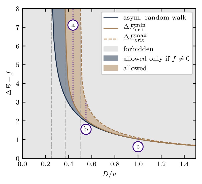
Figure 3: Dynamical phase diagram with bounds on the affinity depending on the ratio $D/v$ between diffusion coefficient and mean velocity. The region between $\Delta E_{\mathrm{crit}}^{\mathrm{min}}$ and $\Delta E_{\mathrm{crit}}^{\mathrm{max}}$ is accessible for any value of the pulling force $f$. The region below $\Delta E_{\mathrm{crit}}^{\mathrm{min}}$ can only be reached if the strand is pulled outwards with $f\neq 0$. A global lower bound on the affinity is given by the curve generated by an asymmetric random walk. For vanishing $f$ a stronger bound can be obtained that separates both regions. There is also a global upper bound to the affinity. The global lower bound diverges at $D/v=1/4$; the lower bound for $f=0$ diverges at $D_{0}/v_{0}=3/8$ and the global upper bound diverges at $D/v=1/2$. The three different cases of $D/v$ that are studied in more detail in Fig. 2 are marked with dotted lines.

The fact that there have to be bounds on the binding energy under the constraint of a given value of the velocity and diffusivity could also be anticipated as a consequence of a more general bound on the diffusion coefficient introduced in barato_thermodynamic_2015 ; pietzonka_universal_2016 that bounds the Fano factor, i. e. , $2D/v$, through the affinity $\mathcal{A}$ and the number of states $N$ (in our case two)

$$\frac{1}{2N}\coth\left(\frac{\mathcal{A}}{2N}\right)\leq\frac{D}{v}\leq\frac{1}{2}\coth\left(\frac{\mathcal{A}}{2}\right)\,.$$ (14)

These bounds are valid for any set of parameters, so they are in particular applicable to the situation without pulling force considered above. In this case, we have to replace $v$ and $D$ by $v_{0}$ and $D_{0}$, respectively.

Without the pulling force, the affinity is equal to the binding energy, i. e. , $\mathcal{A}=\Delta E$. Obviously, the upper bound in Eq. (14) leads to the same upper bound on the binding energy as in Eq. (12).

For the lower bound, however, the resulting bound on the binding energy

$$\Delta E\geq 4\mathop{\mathrm{arcoth}}\left(\frac{4D_{0}}{v_{0}}\right)$$ (15)

is weaker than the one found in Eq. (11). This can be explained by the fact that equality holds in the left inequality in Eq. (14) if and only if the process in question is an asymmetric random walk. Since we set $f=0$, it is not possible to reach an asymmetric random walk with the remaining parameters without having $v_{0}=0$ and thereby invalidating the bound. The bound in Eq. (11) represents the state closest to an asymmetric random walk with finite velocity and $f=0$. This behavior is illustrated in Fig. 3, where the accessible region of the affinity is shown depending on the ratio of diffusion coefficient to mean velocity. The region between $\Delta E_{\mathrm{crit}}^{\mathrm{min}}$ and $\Delta E_{\mathrm{crit}}^{\mathrm{max}}$ contains the possible values of $\Delta E$ for fixed $D_{0}/v_{0}$. For arbitrary values of $f$ the accessible region is larger and restricted by the curve that corresponds to an asymmetric random walk with the respective ratio $D/v$. In this diagram, we also mark the three different parameter values that we used to illustrate the general behavior of the mean velocity and the diffusion constant in Sec. II.4.

III Classical translocation ratchet

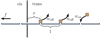
Figure 4: Schematic depiction of a translocation ratchet. The position of the strand is encoded in the distance $x$ of the pore from the closest binding site on the trans side. Each empty binding site gets occupied with rate $w_{\mathrm{on}}$ and each occupied site is emptied with rate $w_{\mathrm{off}}$.

While the simplistic model of an asymmetric random walk with alternating rates is able to capture the main feature of the ratcheting mechanism, namely that it can pull the strand inwards against a force, we will now focus on a more involved model that should give a better description of the actual mechanism that governs DNA uptake as reported in hepp_kinetics_2016 .

The model presented here was originally introduced in peskin_cellular_1993 , where an expression for the mean velocity of the ratchet was derived. We augment this calculation by a general scheme by which not only the mean velocity, i. e. , the first scaled cumulant of the distribution of traveled distance, but in fact all cumulants and especially the diffusion constant can be calculated in a systematic way.

The key idea of this classical model, which is schematically depicted in Fig. 4, is to encode the position of the strand in a cyclical variable $x$ that is the distance of the pore to the closest binding site on the trans side. As before, we use the distance of two neighboring binding sites as the length scale for the mathematical description. This means that $x$ can take values in the range $[0,1)$, where the boundaries represent the state where a new binding site becomes available or vanishes. It is assumed that the dynamics of the position is described by an overdamped Brownian motion and it evolves according to the Langevin equation

$$\dot{x}=-\mu f+\xi(t)\,,$$ (16)

where $\xi(t)$ denotes a delta correlated white noise with $\left\langle\xi(t)\xi(t^{\prime})\right\rangle=2\mathcal{D}\delta(t-t^{\prime})$ with the bare diffusivity $\mathcal{D}$; $f$ is the force pulling on the strand and $\mu=\mathcal{D}$ is the mobility.

The state of the binding site in front of the pore (on the trans side) determines, whether it is possible for the position to cross the periodic boundary and retract the ratchet by one step. Ideally one would have to keep track of the states of all binding sites and forbid the jump from $x=0$ to $1$ whenever the site in front of the pore is occupied and blocks the transition. However, this is not necessary in the case of fast (un)binding rates of the chaperone molecules in which case the binding sites are instantaneously equilibrated. For this reason it is sufficient to forbid a jump from $x=0$ to $1$ with the stationary probability $p_{\mathrm{on}}^{\mathrm{s}}=w_{\mathrm{on}}/(w_{\mathrm{on}}+w_{\mathrm{off}})$ of being in the bound state. Jumps in the opposite direction are always allowed.

The merit of this, perhaps oversimplified, model lies in the fact that it is possible to obtain the stationary distribution of the position in closed form. Based on the stationary distribution it is furthermore possible to determine the mean velocity of the Brownian ratchet as peskin_cellular_1993

$$v=\frac{\mathcal{D}f^{2}}{\frac{\mathrm{e}^{f}-1}{1-K(\mathrm{e}^{f}-1)}-f}\,,$$ (17)

where $K\equiv{w_{\mathrm{off}}}/{w_{\mathrm{on}}}$ denotes the dissociation constant. As a consequence, the stall force is given by

$$f_{0}=\ln\left(1+\frac{1}{K}\right)\,.$$ (18)

While the stationary distribution is sufficient to calculate the mean velocity as already performed in peskin_cellular_1993 , the diffusion coefficient, i. e. , the rate at which the variance of the position is increasing, cannot be calculated from the distribution alone. It is, however, interesting to also compare the diffusion coefficient gained from experimental data with the prediction of this model. For this reason we present a systematic scheme that allows for the iterative calculation of mean velocity, diffusion constant and all higher cumulants.

The calculations are based on the same principles that we used to calculate the diffusion constant in the simple model. In this case, however, it is to our knowledge not possible to calculate the largest eigenvalue $\alpha(\lambda)$ of the tilted operator $\mathcal{L}(\lambda)$ directly. Since we are only interested in the first few derivatives of $\alpha(\lambda)$ at $\lambda=0$, it is possible to expand the largest eigenvalue into a perturbation series and derive an iteration formula for the cumulants. The details of this expansion are explained in Appendix A. In the specific case of the Brownian ratchet, the calculation is additionally complicated by the somewhat unusual form of periodic boundary conditions for the position variable $x$ that prevent us from directly applying known results for the tilted operator touchette_introduction_2018 .

Nevertheless, it is possible to obtain the tilted operator and perform all necessary calculations through discretization of the state space. The procedure is quite technical, which is why it is not presented here. The interested reader is referred to appendix B. Here, we only present the final result for the diffusion coefficient in the classical model of a Brownian ratchet that constitutes one of the main results of this paper. The diffusion coefficient is given by

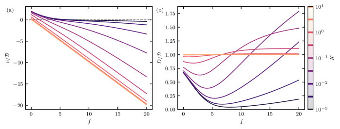
Figure 5: Mean velocity (a) and diffusivity (b) of the classical Brownian ratchet. For large $K$, mean velocity and diffusivity resemble results for diffusion without a ratcheting mechanism, i. e. , $v=-\mathcal{D}f$ and $D=\mathcal{D}$ since the stationary probability for a chaperone to be bound gets smaller as $K$ grows. Therefore, fewer transitions across the periodic boundary are rejected for large $K$. For small $K$ the movement is affected by the chaperones and we see a plateau developing in the $f$ dependence of $v$. For small $f$ the strand is pulled to the trans side. With decreasing $K$ the diffusion coefficient develops a minimum and a maximum. The minimum stays roughly at the stall force while the maximum that is larger than the bare diffusivity moves to large $f$ as $K$ decreases.

$$D=\frac{\mathcal{D}f^{2}}{2\left(Kf\mathrm{e}^{f}-Kf-f+\mathrm{e}^{f}-1\right)^{3}}\,G(f,K)\,,$$ (19)

where the function $G(f,K)$ is given by the expression

$$G(f,K)\equiv (\mathrm{e}^{f}-1)^{3}[2K^{3}f+6K^{2}+K]$$

$$+(\mathrm{e}^{f}-1)^{2}[-6K^{2}f+4Kf-10K+1]$$

$$+(\mathrm{e}^{f}-1)[10Kf-4f+6]-6f\,.$$ (20)

Figure 5 shows the mean velocity and the diffusivity for different dissociation constants $K$ as a function of the force $f$. For $K\gg 1$ it is increasingly unlikely to find a bound chaperone that stalls the movement. Consequently, the system behaves as if no ratcheting mechanism were present and we find $v\approx-\mathcal{D}f$ and $D\approx\mathcal{D}$. If $K$ is small, however, the effects of the chaperones on the diffusion get more pronounced.

From the results for mean velocity and diffusion coefficient, it is possible to determine how the system behaves in the limit of strong pulling force. We find that the mean velocity diverges for $f\rightarrow\infty$, whereas the ratio of velocity to force converges to

$$\lim_{f\rightarrow\infty}\frac{v}{f}=-\mathcal{D}\,,$$ (21)

which resembles the mobility we would have expected if no ratcheting mechanism were present. The same is true for the diffusion coefficient that approaches

$$\lim_{f\rightarrow\infty}D=\mathcal{D}\,.$$ (22)

This means that, in the classical model, strong pulling forces negate the effect of the ratcheting mechanism. This result is counterintuitive since one would expect that the ratchet can stall the translocation also for large forces and consequently there should be an impact on velocity and diffusion coefficient similar to the effect we found in the simple model. As it turns out, the results from Eqs. (21) and (22) are only valid if the limit $w_{\mathrm{on}},w_{\mathrm{off}}\rightarrow\infty$ is performed first, which is the main assumption of the classical model.

IV Translocation ratchet with memory

IV.1 The model

The established classical model from peskin_cellular_1993 has the drawback that it is only valid in the limit of fast binding and unbinding because it does not keep track of the state of the individual binding sites. Instead, the state of a site is drawn from the stationary distribution as needed. For finite binding rates this strategy is not justified, since the binding sites are always empty when they enter the solution through the pore and are therefore not in chemical equilibrium with the surrounding.

Ideally one would have to incorporate the state and dynamics of each binding site into the model and determine whether a site can cross through the pore back to the cis side based on the state of the specific site in front of the pore on the trans side. For a chain of finite length this approach has been used to determine the mean translocation time from simulations in liebermeister_ratcheting_2001a . This treatment, however, is not viable for long chains since the state space grows exponentially with the number of binding sites taken into account.

One can, however, assume that sites far away from the membrane are in chemical equilibrium since they did not interact with the wall for a time longer than their equilibration time. For this reason, it is only necessary to incorporate a finite number of sites into the model in order to obtain a satisfactory result.

Following these considerations, we propose a modified model that is defined as follows: As in the classical case the position of the strand is represented by a continuous variable $x$ but is augmented by the state of the first $m$ sites on the trans side, which act as a memory that we denote with $M$. As in the case without memory, the position $x$ can take values from the interval $[0,1)$ and evolves according to the Langevin equation (16).

Each bit of the memory represents the state of one binding site, where we use 1 to represent the bound state that cannot pass through the pore and 0 corresponds to the unbound state. The leftmost bit is the site closest to the pore. Since binding and unbinding occur randomly with the rates $w_{\mathrm{on}}$ and $w_{\mathrm{off}}$, each bit of the memory flips from one state to the other according to Markovian dynamics with these rates.

The memory and position are only coupled when $x$ attempts to diffuse across the periodic boundary. A jump from $x=0$ to $1$ means that a binding site from the trans side moves into the pore. This process is only possible if the site is unoccupied. So if the leftmost bit of $M$ is 1, the jump of $x$ is rejected. If the leftmost bit is $0$, the position variable can cross the boundary and the memory is shifted by one bit to the left. To keep the length of the memory constant, the rightmost bit is filled with a state drawn from the stationary distribution. We thereby assume that this binding site is sufficiently far away from the pore that it had time to reach chemical equilibrium.

A jump of $x$ in the opposite direction is always possible. If such a jump occurs, the bits of the memory are shifted to the right and the leftmost bit is filled with a 0 since every site is unoccupied upon entering the trans side. The transition probabilities from one memory state to another when a jump across the periodic boundary is attempted are depicted in Fig. 6, where the boxes represent the state of the memory.

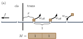
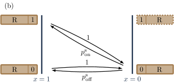
Figure 6: Model with memory. The state of the first $m$ binding sites after the pore on the trans side are incorporated into the description as it is indicated in panel (a) by a box that represents the state of a two-bit memory. Panel (b) illustrates the transition rules across the periodic boundary. The figure shows the state of the memory before and after the jump. When the position $x$ crosses the boundary from 1 to 0, the memory gets shifted to the right and the first bit is filled with 0. Movement in the opposite direction is only possible if the memory starts with 0. In this case the memory is shifted to the left and the rightmost bit is filled randomly according to the stationary distribution of the bound or unbound state. $R$ denotes the $(m-1)$ remaining bits of the memory that get shifted by the jump across the periodic boundary.

IV.2 Results

For this model, the calculation of mean velocity and diffusion coefficient is much more involved than for the previous models since we have to deal with the coupled dynamics of both the memory and the position variable $x$. An analytical calculation as it is done in Appendix B for the classical model is, to our knowledge, no longer feasible. One can, however, discretize the state space and solve the systems of linear equations that correspond to Eqs. (39) numerically.

Figure 7 shows a comparison of the mean velocity and the diffusion coefficient predicted by the Brownian ratchet model with and without memory. The parameters were chosen in such a way that the results match the experimental findings presented in hepp_kinetics_2016 up to scaling of the axes.

Since we no longer assume timescale separation between the diffusion and binding process, the binding rate $w_{\mathrm{on}}$ and the unbinding rate $w_{\mathrm{off}}$ enter the model separately. To keep the parameters consistent with hepp_kinetics_2016 , where their ratio was found as $K=0.0012$, we choose $w_{\mathrm{on}}=1000\,\nicefrac{\mathrm{1}}{\mathrm{s}}$ and $w_{\mathrm{off}}=1.2\,\nicefrac{\mathrm{1}}{\mathrm{s}}$. The bare diffusivity $\mathcal{D}$ fixes the timescale of the diffusion of the strand. The fact that the experimental data are matched quite well by the prediction of the classical model without memory indicates that the assumption of a timescale separation between diffusion and (un)binding is at least approximately valid. To reflect this fact, we choose $\mathcal{D}=1\,\nicefrac{\mathrm{1}}{\mathrm{s}}$, which is smaller than both rates. Note that the diffusivity has the unit of a frequency since we set the distance of two neighboring sites to unity.

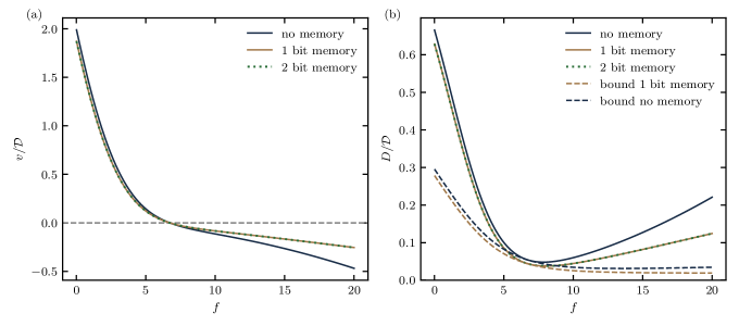
Figure 7: Comparison of velocity (a) and diffusivity (b) in the model proposed in peskin_cellular_1993 and in our model with memory that incorporates the state of the first few binding sites. The parameters were chosen such that the prediction of the classical model matches the experimental findings from hepp_kinetics_2016 up to rescaling of the axes. It is evident that the two models deviate most strongly for high pulling forces while the stall force is the same in both cases. The plot in the right panel shows the diffusion constant for both models as well as a lower bound following as a consequence of the thermodynamic uncertainty relation. Parameters: $\mathcal{D}=1\,\nicefrac{\mathrm{1}}{\mathrm{s}}$, $w_{\mathrm{on}}=1000\,\nicefrac{\mathrm{1}}{\mathrm{s}}$, $w_{\mathrm{off}}=1.2\,\nicefrac{\mathrm{1}}{\mathrm{s}}$.

It is evident that the introduction of memory into the model leads to slower average speed of the strand both when the force is below the stall force and the strand is pulled inside by the ratcheting mechanism and also for forces above the stall force when the strand is pulled out. These two effects are both caused by the memory but in a slightly different way.

Each binding site that enters the trans side is initially empty. This means that the probability to find a bound site right in front of the pore is lower than the equilibrium value $p_{\mathrm{on}}^{\mathrm{s}}$. As a result the sites can diffuse back to the cis side with a higher frequency than assumed in the model without memory, leading in turn to smaller $v$.

With increasing $f$ and especially above the stall force this effect becomes less and less relevant since it becomes more and more unlikely that an empty binding site can diffuse from the cis to the trans side. Instead, we find that the memory also decreases the mean velocity when the strand is pulled out. In this case the difference between the two models can be explained by the fact that in the model without memory the decision whether a site can pass through the pore on each attempt is independent from the last attempt. If there is no timescale separation between the binding dynamics of the chaperone molecules and the diffusion of the strand, the outcome of successive attempts to cross the periodic boundary should, however, be correlated. If a chaperone blocks one attempt to diffuse outward, it will also block all attempts in the future unless it unbinds. Introducing the memory into the model makes it possible to capture this behavior.

The comparison of the force dependence of the diffusion coefficient presented in Fig. 7 shows that the memory leads to a smaller diffusivity throughout. The effect is especially pronounced for forces well above the stall force. It is interesting to note that even the introduction of one single bit of memory changes the behavior. The classical model does not even keep track of the binding site right in front of the pore, but instead draws its state from the stationary distribution every time it is needed, which leads to differences in the mean velocity. The figure also shows lower bounds on the diffusion coefficient that are obtained using the thermodynamic uncertainty relation (see also section IV.6).

IV.3 Velocity in the limit of strong driving

One of the key differences between the model with and without memory is that the predicted mean velocity differs vastly when the pulling force is large. In the classical model, which does not keep track of the states of the binding sites, the velocity diverges to negative infinity in the limit of strong pulling $f\rightarrow\infty$. The numerical results for the model with memory, however, indicate that the velocity approaches a finite value in this regime. The aim of this section is to understand this difference in behavior.

Suppose the pulling force is large. This means that, whenever there is an unoccupied binding site in front of the pore on the trans side, it will immediately get pulled out. As a consequence, the movement of the strand is determined only by the occupation pattern of the binding sites. The pulling is stalled whenever there is an occupied site in front of the pore. Once the blocking chaperone molecule unbinds, the strain advances suddenly to the position of the next site that is bound and so on. From these considerations, it is possible to calculate the mean velocity in the limit $f\rightarrow\infty$. To do so, we need to know the average time during which the movement is stalled by a bound site, which we call $\tau_{\text{b}}$, and the average number of sites $\langle n\rangle$ the strain is advanced if it can move.

The waiting time $\tau_{\text{b}}=1/w_{\mathrm{off}}$ is the inverse of the unbinding rate. The probability to advance by $n$ steps, once the movement becomes possible, is given by

$$p(n)=p_{\mathrm{on}}^{\mathrm{s}}\left(p_{\mathrm{off}}^{\mathrm{s}}\right)^{n-1}$$ (23)

if we assume that the state of each individual site is distributed according to the equilibrium distribution. In the limit of strong pulling this is justified since no empty site can enter from the cis side. From Eq. (23) the average number of steps is obtained as

$$\langle n\rangle =\sum_{n=1}^{\infty}np_{\mathrm{on}}^{\mathrm{s}}\left(p_{\mathrm{off}}^{\mathrm{s}}\right)^{n-1}=\frac{p_{\mathrm{on}}^{\mathrm{s}}}{p_{\mathrm{off}}^{\mathrm{s}}}\frac{\mathrm{d}}{\mathrm{d}a}\sum_{n=0}^{\infty}(ap_{\mathrm{off}}^{\mathrm{s}})^{n}\biggr{|}_{a=1}$$

$$=\frac{p_{\mathrm{on}}^{\mathrm{s}}}{p_{\mathrm{off}}^{\mathrm{s}}}\frac{\mathrm{d}}{\mathrm{d}a}\left(\frac{1}{1-ap_{\mathrm{off}}^{\mathrm{s}}}\right)\biggr{|}_{a=1}=\frac{1}{p_{\mathrm{on}}^{\mathrm{s}}}\,.$$ (24)

Therefore, the mean velocity will reach

$$v_{\infty}=-\frac{\langle n\rangle}{\tau_{\mathrm{b}}}=-\frac{w_{\mathrm{on}}+w_{\mathrm{off}}}{w_{\mathrm{off}}/w_{\mathrm{on}}}$$ (25)

as $f$ goes to infinity. The minus sign is introduced because the strain is pulled in the negative direction. For finite values of $f$ we expect that the absolute value of the mean velocity is lower than the asymptotic value since it takes the strain a finite amount of time to move to the next stalling position due to friction.

From Eq. (25) it is obvious that $v_{\infty}$ diverges in the situation assumed in the classical model ($w_{\mathrm{on}},w_{\mathrm{off}}\rightarrow\infty$). On the other hand, this means that deviations of experimental data from the predictions of the classical model can be used to infer the (un)binding rates. This behavior is illustrated in Fig. 8. It shows the mean velocity for the same parameters as in Fig. 7 over a larger range of $f$ and for different timescales of the binding and unbinding rates. Also shown are the asymptotic values of the velocity for each case. As the rates increase the mean velocity approaches the result of the model without memory as expected since the timescale separation is the key assumption of the classical model without memory. Also, it takes larger pulling forces to reach the asymptotic value as the rates grow.

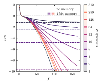
Figure 8: Comparison of the asymptotic behavior of the model with and without memory. Without memory the strain can get pulled out arbitrarily fast as the force $f$ increases. With memory the large $f$ behavior is governed by the timescale introduced by the binding and unbinding rates $w_{\mathrm{on}}$ and $w_{\mathrm{off}}$ entering Eq. (25). The asymptotic values of the velocity are indicated as dashed lines. Parameters: $\mathcal{D}=1\,\nicefrac{\mathrm{1}}{\mathrm{s}}$, $w_{\mathrm{on}}=\omega\cdot 1000\,\nicefrac{\mathrm{1}}{\mathrm{s}}$, $w_{\mathrm{off}}=\omega\cdot 1.2\,\nicefrac{\mathrm{1}}{\mathrm{s}}$

IV.4 Minimum memory length

The key assumption in the ratchet model with memory is that the last bit of the memory, representing the binding site farthest away from the pore, is always in chemical equilibrium with the surrounding. Whether this is actually the case depends on the system parameters and especially on the length of the memory. This section is concerned with the question of how many sites have to be modeled explicitly to satisfy the assumption mentioned above.

If a specific binding site is already in chemical equilibrium, so is its right neighbor. For this reason, the prediction of the memory model should converge with increasing memory length $m$. For the parameter values used in Fig. 7, one bit of memory is already sufficient since the addition of a second bit (shown as a dotted line) does not change the result significantly. To calculate the minimum memory length $m_{\mathrm{min}}$ for a broader set of parameters, we calculated the velocity for different (un)binding rates for pulling forces in the range from zero to twenty. The results obtained for the specific choice of $\mathcal{D}=1$ are universal, since any other choice can be realized by rescaling in time. As a criterion for sufficient convergence, we checked whether increasing the memory size by one bit changes the result by more than 5% for any $f$. The resulting minimal memory length as a function of the rates is shown in Fig. 9.

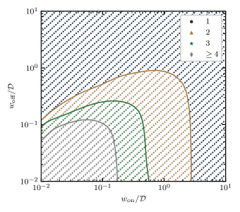
Figure 9: Minimum number of memory bits needed to accurately model the ratcheting mechanism as a function of the binding and unbinding rate. Interpolated boundaries between regions with different minimal memory length are added as guide to the eye.

Note that we only compare variants of the model with memory of different lengths $m$ to each other. Whether the classical model without memory is sufficient depends strongly on the driving force, since the classical model predicts a fundamentally different large $f$ behavior, as we have seen in Sec. IV.3. Models with memory but different $m$ show the same asymptotics in $f$ but differ for small forces.

The plot shows that if either the binding or the unbinding rate becomes too small, an additional bit of memory is required. The shaded areas have approximately rectangular shape, which means that the minimum number of bits is roughly determined by a weighted maximum of the binding and the unbinding rate.

IV.5 Affinity and stall force

The goal of this section is to determine the affinity, i. e. , the entropy production of one step of the Brownian ratchet with or without memory. The entropy production is the logarithmic ratio of the probability to observe a trajectory and the probability to observe the time reversed trajectory. Setting the affinity to zero and solving for the driving force allows us to calculate the stall force.

First, we specify what we mean exactly by one step of the ratchet. Suppose the system starts at position $x_{0}$ and the memory is in state $M$. After some time it reaches the ratcheting position $x=1$ with the memory in state $M^{\prime}$. The jump across the periodic boundary changes the memory state to $M^{\prime\prime}$ according to the rules of the model. Afterwards, the system diffuses back to position $x_{0}$ without crossing the periodic boundary and the memory reverts to $M$. Because the dynamics is Markovian and the memory and the position evolve independently of each other, as long as the position does not try to cross the periodic boundary, it is possible to split the affinity into contributions associated to different sections of this trajectory.

On its way from the initial position $x_{0}$ to $x=1$ the position contributes $\mathcal{A}_{x,1}=(x_{0}-1)f$ entropy production. The entropy production stemming from the memory during this section is determined by the difference of bound sites. For each bit that flips from 0 to 1, the entropy production increases by $\ln(w_{\mathrm{on}}/w_{\mathrm{off}})=\Delta E$. If we use $n$ to denote the number of bound sites in $M$ and $n^{\prime}$ for the bound sites in $M^{\prime}$, the entropy production in the memory reads $\mathcal{A}_{M\rightarrow M^{\prime}}=(n^{\prime}-n)\Delta E$. For the same reasons, the entropy production through the position and memory aggregated after the jump across the boundary are $\mathcal{A}_{x,2}=-x_{0}f$ and $\mathcal{A}_{M^{\prime\prime}\rightarrow M}=(n-n^{\prime\prime})\Delta E$, respectively.

The jump across the periodic boundary also leads to a crucial contribution to the entropy production since a jump in one direction is not as likely as the jump in the backwards direction. Here, we have to distinguish between two cases: Either the memory before the jump ends with a zero or a one. In either case the logarithmic ratio of forward to backwards probability is $\mathcal{A}_{\mathrm{jump,i}}=-\ln p_{i}^{\mathrm{s}}$, where $i$ is the last bit of $M^{\prime}$. Depending on $i$, the number of bound bits may be changed through the jump. If $i=1$, the memory shift reduces the number of bound bits by one since the first site is always unbound after the jump. For this reason, we find in this case $n^{\prime\prime}=n^{\prime}-1$. In the case of an unbound last site, the number of bound sites stays untouched, leading to $n^{\prime\prime}=n^{\prime}$.

Summing up, we find that the total affinity of one step is given by

$$\mathcal{A}=-f+\left\{\begin{array}[]{ll}-\ln p_{\mathrm{on}}^{\mathrm{s}}+\Delta E&\mathrm{for}\;i=1\\ -\ln p_{\mathrm{off}}^{\mathrm{s}}&\mathrm{for}\;i=0\end{array}\right.\,.$$ (26)

Using the dependence of the stationary distribution on the binding energy $\Delta E$, one can easily show that both cases yield the same result

$$\mathcal{A}=\ln\left(\exp(\Delta E)+1\right)-f\equiv\Delta\mathcal{F}-f\,,$$ (27)

where we identified the free energy difference $\Delta\mathcal{F}$ associated with the insertion of one binding site in equilibrium with the chemostat that has been previously identified in a similar context in ambjornsson_chaperone-assisted_2004 .

The free energy difference introduced in (27) can be split into a term representing the average change in binding energy caused by an additional binding site and a term representing the change in configuration entropy

$$\Delta\mathcal{F}=p_{\mathrm{on}}^{\mathrm{s}}\Delta E-p_{\mathrm{off}}^{\mathrm{s}}\ln p_{\mathrm{off}}^{\mathrm{s}}-p_{\mathrm{on}}^{\mathrm{s}}\ln p_{\mathrm{on}}^{\mathrm{s}}\,.$$ (28)

This form of the free energy difference makes it especially clear that the strand is pulled in, even if the binding energy of the chaperones vanishes, due to the increase in entropy in the memory. Conversely, to pull out one binding site one has to delete information from the memory, which, according to Landauer’s principle, comes at an energetic cost. In the case $\Delta E=0$ we indeed have $\Delta\mathcal{F}=\ln 2$ as it is to be expected. So in some sense a Brownian ratchet can be seen as a stochastical information processing machine that can erase from or write bits to a memory (see also mandal_work_2012 ; barato_autonomous_2013 for further examples of such devices).

The stall force follows trivially from the condition that the affinity vanishes, leading to

$$f_{0}=\Delta\mathcal{F}\,.$$ (29)

Incidentally, this is the same result as already obtained in peskin_cellular_1993 for the classical model without memory.

IV.6 Thermodynamics and efficiency

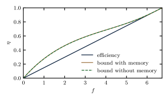
Figure 10: Efficiency of the Brownian ratchet and upper bound derived from the classical model with and without memory. The bound becomes tight for forces close to the stall force. The difference between the models with and without memory is barely visible since they only deviate significantly for forces well above the stall force, where the motor does not perform work.

The analysis of the previous section showed that the Brownian ratchet can be seen as a kind of molecular motor that uses the free energy $\Delta\mathcal{F}$ gained by providing an additional binding site to perform a certain amount of work $\Delta w=f$. It is therefore natural to identify the efficiency $\eta$ of the Brownian ratchet as the ratio of the performed work to the maximum possible amount, i. e. ,

$$\eta\equiv\frac{\Delta w}{\Delta\mathcal{F}}=\frac{1}{1+\mathcal{A}/f}\leq 1\,.$$ (30)

The thermodynamic uncertainty relation that was recently conjectured barato_thermodynamic_2015 ; pietzonka_universal_2016 based on extensive numerical evidence and later proven gingrich_dissipation_2016 ; horowitz_proof_2017a implies a boundary on the efficiency that only relies on the observable quantities $v$, $D$ and $f$ pietzonka_universal_2016a .

The uncertainty relation states that precision, i. e. , low diffusion $D$ comes at the cost of high dissipation. For the system at hand, it can be stated in the form

$$\frac{D}{v}\mathcal{A}\geq 1\,.$$ (31)

This relation has a number of consequences regarding the force dependence of mean velocity and diffusion coefficient.

Since the affinity of a step of the ratchet is known [see Eq. (27)], it is possible to derive a lower bound on the diffusion coefficient by solving Eq. (31) for $D$. The resulting bounds are shown as dashed lines in Fig. 7. Since the bound becomes tight in the linear response regime and close to the stall force, it allows also for the calculation of the diffusion coefficient at stall force:

$$D_{\mathrm{stall}}=\lim_{f\rightarrow f_{0}}\frac{v(f)}{\Delta\mathcal{F}-f}=-\left.\frac{\partial v(f)}{\partial f}\right|_{f=f_{0}}\,.$$ (32)

In terms of the efficiency of the ratchet the uncertainty relation is expressed in the inequality

$$\eta\leq\frac{1}{1+\frac{v}{Df}}\,.$$ (33)

The efficiency as well as the bounds derived from the model with or without memory are shown in Fig. 10. As expected, the bound becomes tight in the linear response regime and close to the stall force.

V Summary

We have analyzed the force dependence of the diffusion coefficient for three different models of Brownian ratchets with varying degree of complexity. For the first model that describes the ratcheting mechanism in terms of an asymmetric random walk with an alternating set of rates one can obtain the scaled cumulant generating function in closed form. We derived a bound for the Fano factor at vanishing pulling force that is stronger than the bound obtained from the thermodynamic uncertainty relation. For this model we identified different regimes in the parameter space. Depending on the regime the force dependence of the diffusion coefficient can develop a local minimum.

For a classical model for the Brownian ratchet that was first introduced in peskin_cellular_1993 and has been found to explain DNA uptake by Neisseria gonorrhoeae bacteria hepp_kinetics_2016 , we derived an expression for the diffusion coefficient. This new result could in the future be used for comparison with experimental data.

The classical model is based on the assumption that the binding and unbinding of the chaperones are fast compared to the diffusion process. We found that the large $f$ behavior does not match the expectation of a ratcheted process, due to this timescale separation. In order to overcome the limitations of the classical model we introduced a memory into the model that allowed us to numerically calculate predictions for the force dependence of mean velocity and diffusion coefficient in the case where there is no clear timescale separation. Here we found that the mean velocity approaches a finite value as $f$ increases, as one would expect from naive considerations. We could identify the stall force for the model with memory and found that it matches the result of the model without memory. We also analyzed how many bits of memory are needed for the results to converge to their respective values if an infinite memory were used. We found, in accordance with our expectations, that the more memory is needed the slower the (un)binding process is. Conversely, we confirmed that in the limit of infinitely fast (un)binding no memory is needed at all.

We identified the thermodynamic efficiency of the ratchet and illustrated how one can use the measurable quantities $v$, $D$, and $f$ to bound the efficiency from above. This bound is a consequence of the thermodynamic uncertainty relation and becomes tight for forces around the stall force.

Appendix A Systematic scheme for the calculation of cumulants of integrated currents

In this appendix, we recall a general formalism that can be used to determine the diffusion coefficient in Markov processes like the models for Brownian ratchets considered in this paper koza_general_1999 . It is based on methods commonly used in the field of large deviations touchette_large_2009 . The mean velocity, the diffusion coefficient and in fact all rescaled cumulants of the distribution of the traveled distance are encoded in the rescaled cumulant generating function

$$\alpha(\lambda)\equiv\lim_{t\rightarrow\infty}\frac{1}{t}\ln\left\langle\mathrm{e}^{\lambda\Delta x}\right\rangle$$ (34)

as its derivatives at $\lambda=0$. Expanding the generating function in a Maclaurin series up to second order yields

$$\alpha(\lambda)=v\lambda+D\lambda^{2}+\mathcal{O}(\lambda^{3})\,.$$ (35)

The generating function can be obtained as the Perron-Frobenius eigenvalue of the so called tilted operator that generates the evolution of the moment generating function conditioned on the final state of the trajectory

$$g(\lambda,x,t)\equiv\left\langle\mathrm{e}^{\lambda\Delta x}\right\rangle_{x}\,,$$ (36)

where we use the notation $\left\langle\cdot\right\rangle_{x}$ to denote an average over all trajectories that end in the state $x$. The time evolution of this quantity is given by

$$\partial_{t}g(\lambda,x,t)=\mathcal{L}(\lambda)g(\lambda,x,t)\,,$$ (37)

where the tilted operator $\mathcal{L}(\lambda)$ is a differential operator acting on the state argument of $g(\lambda,x,t)$. In the case of $\lambda=0$ the tilted operator is identical to the Fokker-Planck or master operator $\mathcal{L}_{0}$ generating the time evolution of the probability distribution. Typically, the eigenvalue problem leading to the generating function cannot be obtained in closed form. The cumulants, however, can be calculated iteratively by expanding the eigenvalue equation in orders of $\lambda$. To this end, we insert the expansions

$$\mathcal{L}(\lambda) =\mathcal{L}_{0}+\mathcal{L}_{1}\lambda+\mathcal{L}_{2}\lambda^{2}+\mathcal{O}(\lambda^{3})$$ (38a)

$$\mathbf{q}(\lambda) =\mathbf{p}^{\mathrm{s}}+\mathbf{q}_{1}\lambda+\mathbf{q}_{2}\lambda^{2}+\mathcal{O}(\lambda^{3})$$ (38b)

into the eigenvalue equation $\mathcal{L}(\lambda)\mathbf{q}(\lambda)=\alpha(\lambda)\mathbf{q}(\lambda)$, sort by orders of $\lambda$, and arrive at

$$\mathcal{L}_{0}\mathbf{p}^{\mathrm{s}} =0\,,$$ (39a)

$$\mathcal{L}_{0}\mathbf{q}_{1}+\mathcal{L}_{1}\mathbf{p}^{\mathrm{s}} =v\mathbf{p}^{\mathrm{s}}\,,$$ (39b)

$$\mathcal{L}_{1}\mathbf{q}_{1}+\mathcal{L}_{0}\mathbf{q}_{2}+\mathcal{L}_{2}\mathbf{p}^{\mathrm{s}} =D\mathbf{p}^{\mathrm{s}}+v\mathbf{q}_{1}\,.$$ (39c)

Since the constant function denoted by the vector $\bra{1}$ is a left eigenvector to the Markov operator $\mathcal{L}_{0}$ with corresponding eigenvalue zero, the solutions of these linear equations are not unique. They become unique, if we additionally demand that they are normalized, i. e. , $\braket{1}{\mathbf{p}^{\mathrm{s}}}=1$ and $\braket{1}{\mathbf{q}_{1}}=\braket{1}{\mathbf{q}_{2}}=0$, where $\braket{\cdot}{\cdot}$ denotes the standard scalar product. To calculate velocity and diffusion coefficient, we multiply equations (39b) and (39c) by $\bra{1}$ from the left and use $\bra{1}\mathcal{L}_{0}=0$, leading to

$$v =\Braket{1}{\mathcal{L}_{1}}{\mathbf{p}^{\mathrm{s}}}$$ (40a)

$$D =\Braket{1}{\mathcal{L}_{1}}{\mathbf{q}_{1}}+\Braket{1}{\mathcal{L}_{2}}{\mathbf{p}^{\mathrm{s}}}$$ (40b)

Numerically this set of equations can be solved by projection of the vectors and operators in an appropriate set of basis vectors and solving the corresponding set of linear equations.

Appendix B Calculation of the diffusion coefficient in the classical model

In this appendix, we derive a closed-form expression for the diffusion coefficient in the classical model for a Brownian ratchet without memory. To this end, we aim to solve Eqs. (40) that allow us to calculate the diffusion coefficient using the tilted operator $\mathcal{L}(\lambda)$.

The boundary condition used in peskin_cellular_1993 states that transitions from the left border of the region at $x=0$ to the right border at $x=1$ are rejected with probability $p_{\mathrm{on}}^{\mathrm{s}}$, while transitions in the opposite direction are always allowed. This rather unorthodox form of a periodic boundary condition cannot be intuitively expressed in terms of a continuous description of the state space. To circumvent this issue, we discretize the state space, perform all necessary calculations, and take the limit of infinitely small discretization at the end.

B.1 Discretization

We split the state space into $N$ discrete points separated by the distance $h=1/N$. Therefore each continuous function $\psi(x)$ is approximated by the $N$-dimensional vector $\psi_{i}\equiv\psi(x_{i})$ with $x_{i}=ih$. In this picture, the time evolution of the probability distribution $p_{i}$ is given by the master equation

$$\partial_{t}p_{i}=(\mathcal{L}_{0}p)_{i}\equiv p_{i-1}\left(-\frac{\mathcal{D}f}{2h}+\frac{\mathcal{D}}{h^{2}}\right)+p_{i+1}\left(\frac{\mathcal{D}f}{2h}+\frac{\mathcal{D}}{h^{2}}\right)\\ -p_{0}\left(\frac{2\mathcal{D}}{h^{2}}\right)\quad i\not\in\{1,N\}$$ (41)

that approximates the Fokker-Planck equation inside the interval $(0,1)$. Due to the nature of the boundary conditions, the states at the boundary of the interval need special treatment.

Because jumps from $x=0$ to $1$ are rejected with probability $p_{\mathrm{on}}^{\mathrm{s}}$, the rate corresponding to jumps in this direction is diminished, leading to

$$({L}_{0}p)_{N}=p_{N-1}\left(-\frac{\mathcal{D}f}{2h}+\frac{\mathcal{D}}{h^{2}}\right)\\ +p_{1}\left(1-p_{\mathrm{on}}^{\mathrm{s}}\right)\left(\frac{\mathcal{D}f}{2h}+\frac{\mathcal{D}}{h^{2}}\right)+p_{N}\left(-\frac{2\mathcal{D}}{h^{2}}\right)\,.$$ (42)

Consequently, the exit rate of state $i=1$ is decreased by the same amount and we find

$$(\mathcal{L}_{0}p)_{1}=p_{N}\left(-\frac{\mathcal{D}f}{2h}+\frac{\mathcal{D}}{h^{2}}\right)+p_{2}\left(\frac{\mathcal{D}f}{2h}+\frac{\mathcal{D}}{h^{2}}\right)\\ -p_{1}\left((2-p_{\mathrm{on}}^{\mathrm{s}})\frac{\mathcal{D}}{h^{2}}-p_{\mathrm{on}}^{\mathrm{s}}\frac{\mathcal{D}f}{2h}\right)\,.$$ (43)

In the discrete picture, we also have to replace integrals by their Riemann sum approximation. So, for example, the normalization condition of the stationary distribution becomes

$$\int_{0}^{1}p^{\mathrm{s}}(x)\,\mathrm{d}x\approx h\sum_{i=1}^{N}p^{\mathrm{s}}_{i}=1\,.$$ (44)

B.2 Tilted operator

The first step in our derivation is the identification of the tilted operator $\mathcal{L}(\lambda)$, or to be more precise, the Taylor expansion of this operator up to second order in $\lambda$.

While the boundary conditions prevent us from using known results for the tilted operator in continuous state space, we can use the general result

$$\mathcal{L}(\lambda)_{i,j}=\mathcal{L}_{0,i,j}\exp(d_{j,i}\lambda)$$ (45)

for a discrete state space, where the distance matrix is given by $d_{i,j}=h(\delta_{i,j+1}-\delta_{i,j-1})$.

Expanding this expression into a Taylor series, we find

$$\mathcal{L}_{1,i,j}=\mathcal{L}_{0,i,j}d_{j,i}$$ (46)

and

$$\mathcal{L}_{2,i,j}=\mathcal{L}_{0,i,j}d_{j,i}^{2}/2\,.$$ (47)

Now we discuss how these operators act on a test function $\psi(x)$ in the continuous limit.

B.2.1 First order

For the first order coefficient, we arrive at

$$(\mathcal{L}_{1}\psi)_{i}=\psi_{i-1}\left(-\frac{\mathcal{D}f}{2}+\frac{\mathcal{D}}{h}\right)-\psi_{i+1}\left(\frac{\mathcal{D}f}{2}+\frac{\mathcal{D}}{h}\right)\\ =-\mathcal{D}f\frac{\psi_{i+1}+\psi_{i-1}}{2}-\mathcal{D}\frac{\psi_{i+1}-\psi_{i-1}}{h}\,,$$ (48)

which converges in the limit $h\rightarrow 0$ to the known result for a continuous state space that is given by

$$\mathcal{L}_{1}=-\mathcal{D}(f+2\partial_{x})\,.$$ (49)

At the boundary the situation is, again, more subtle, since the rates are modified and we also have to take into account that the function the operator is acting on may jump across the periodic boundary. Here, we find the relations

$$(\mathcal{L}_{1}\psi)_{1}=-\mathcal{D}f\frac{\psi_{N}+\psi_{1}}{2}+\frac{\mathcal{D}}{h}\left(\psi_{N}-\psi_{1}\right)$$ (50)

at the lower bound of the interval and

$$(\mathcal{L}_{1}\psi)_{N}=-\frac{\mathcal{D}f}{2}\left[\left(1-p_{\mathrm{on}}^{\mathrm{s}}\right)\psi_{1}+\psi_{N}\right]\\ +\frac{\mathcal{D}}{h}\left[-\left(1-p_{\mathrm{on}}^{\mathrm{s}}\right)\psi_{1}+\psi_{N}\right]$$ (51)

at the upper boundary. Both expressions contain terms that may diverge if we take the continuous limit. Note that if $\psi(x)$ obeys the boundary condition $\psi(1)=(1-p_{\mathrm{on}}^{\mathrm{s}})\psi(0)$ that holds for the stationary distribution, the value at the upper bound stays finite while the value at the lower bound diverges.

The apparent problem of possibly diverging values of $\mathcal{L}_{1}\psi$ can be resolved by the fact that they are only ever needed inside of integrals. Since the divergence is of order $1/h$, the result of the integral converges if we let $h$ go to zero. However, additional terms introduced by the divergences at the boundaries have to be taken into account.

Combining the action of the operator $\mathcal{L}_{1}$ inside the interval and on its boundaries, we obtain the integration rule

$$\int_{0}^{1}\mathcal{L}_{1}\psi\,\mathrm{d}x=-\int_{0}^{1}\mathcal{D}(f\psi+2\psi^{\prime})\,\mathrm{d}x+2\mathcal{D}\left[\psi(1)-\psi(0)\right]\\ +p_{\mathrm{on}}^{\mathrm{s}}\mathcal{D}\psi(0)=-\mathcal{D}f\int_{0}^{1}\psi\,\mathrm{d}x+\mathcal{D}p_{\mathrm{on}}^{\mathrm{s}}\psi(0)$$ (52)

that will become useful for the evaluation of the mean velocity and the diffusion coefficient according to Eqs. (40a) and (40b), respectively.

B.2.2 Second order

For the second order coefficient of the expansion of the tilted operator, we perform calculations along the same line as for the first order and find that the discretization

$$(\mathcal{L}_{2}\psi)_{i}=\frac{1}{2}\left[\psi_{i-1}\left(-\frac{\mathcal{D}f}{2}h+\mathcal{D}\right)+\psi_{i+1}\left(\frac{\mathcal{D}f}{2}h+\mathcal{D}\right)\right]$$ (53)

converges in the continuous limit. Inside the interval, where the test function is continuous, the operator acts as a scalar, allowing us to identify

$$\mathcal{L}_{2}=\mathcal{D}\,.$$ (54)

While this is not the case at the boundaries, it is obvious that the values of $(\mathcal{L}_{2}\psi)_{1}$ and $(\mathcal{L}_{2}\psi)_{N}$ stay finite in the limit $h\rightarrow 0$ even if the test function jumps. Since $\mathcal{L}_{2}\psi$ also appears only inside integrals, these deviations do not affect the result.

B.3 Calculation of the cumulants

Now that we know how the operators $\mathcal{L}_{i}$ act, we are able to iteratively calculate the scaled cumulants like mean velocity and diffusivity. Plugging the integration rule (52) into Eqs. (40a) and (40b), we find

$$v=\int_{0}^{1}\mathcal{L}_{1}p^{\mathrm{s}}(x)\,\mathrm{d}x=-\mathcal{D}f+\mathcal{D}p_{\mathrm{on}}^{\mathrm{s}}p^{\mathrm{s}}(0)$$ (55)

and

$$D =\int_{0}^{1}\mathcal{L}_{1}q_{1}(x)\,\mathrm{d}x+\int_{0}^{1}\mathcal{L}_{2}p^{\mathrm{s}}(x)\,\mathrm{d}x$$

$$=\mathcal{D}\left[1+p_{\mathrm{on}}^{\mathrm{s}}q_{1}(0)\right]\,.$$ (56)

The last step remaining is the calculation of the stationary distribution and the first order correction of the eigenfunction of the tilted operator $q_{1}(x)$.

B.3.1 Stationary distribution

The stationary distribution is the solution of the stationary Fokker-Planck equation

$$\mathcal{L}_{0}p^{\mathrm{s}}(x)=\mathcal{D}\left[f\partial_{x}+\partial_{x}^{2}\right]p^{\mathrm{s}}(x)=0$$ (57)

obeying the boundary condition $p^{\mathrm{s}}(1)=(1-p_{\mathrm{on}}^{\mathrm{s}})p^{\mathrm{s}}(0)$. This boundary condition was derived peskin_cellular_1993 . It also emerges in a natural way if one considers the discretized Fokker-Planck equation at the boundaries. In order for Eq. (42) to converge to zero, the factors in front of the jump rates have to be equal, which leads to the aforementioned boundary condition.

The differential Eq. (57) has the general solution

$$p^{\mathrm{s}}(x)=c_{1}\exp(-fx)+c_{2}$$ (58)

with the two constants $c_{1}$ and $c_{2}$ that are determined by the boundary condition and the normalization of the stationary distribution. Solving the corresponding set of linear equation yields

$$c_{1} =\frac{fe^{f}}{Kfe^{f}-Kf-f+e^{f}-1}\quad\text{and}$$ (59a)

$$c_{2} =\frac{f\left(Ke^{f}-K-1\right)}{Kfe^{f}-Kf-f+e^{f}-1}\,,$$ (59b)

where we used the relation $p_{\mathrm{on}}^{\mathrm{s}}=1/(1+K)$ to express the stationary distribution of a bound site in terms of the dissociation constant $K=w_{\mathrm{off}}/w_{\mathrm{on}}=\exp(-\Delta E)$.

The mean velocity follows directly from Eq. (55) and is given by

$$v=-\mathcal{D}f+\mathcal{D}p_{\mathrm{on}}^{\mathrm{s}}\left(c_{1}+c_{2}\right)\,.$$ (60)

After inserting the constants into this equation this result matches the one of Peskin et al. peskin_cellular_1993 , found in their original publication by slightly different means.

B.3.2 First order correction

In the next step, we calculate the first order correction to the eigenfunction of the tilted operator that is given by the solution of the inhomogeneous differential equation

$$\mathcal{L}_{0}q_{1}(x)=b(x)\,$$ (61)

where the inhomogeneity is given by

$$b(x)\equiv vp^{\mathrm{s}}(x)-\mathcal{L}_{1}p_{\mathrm{s}}(x)=A\exp(-fx)+B+C\delta(0)\,,$$ (62)

with $C=-A[1-\exp(-f)]/f-B$. The constants $A$ and $B$ are related to the constants appearing in the stationary distribution by the relations

$$A \equiv\mathcal{D}[p_{\mathrm{on}}^{\mathrm{s}}c_{1}(c_{1}+c_{2})-2fc_{1}]\quad\text{and}$$ (63a)

$$B \equiv\mathcal{D}[p_{\mathrm{on}}^{\mathrm{s}}c_{2}(c_{1}+c_{2})]\,.$$ (63b)

As explained earlier, the boundary conditions used in the model lead to a deltalike divergence stemming from the application of the operator $\mathcal{L}_{1}$ to the stationary distribution. This divergence does not need to be taken into account when solving the differential equation. It merely assures that $b(x)$ is zero on average. If this were not the case, one could construct a contradiction by integrating both sides of Eq. (61) over the whole state space. The left hand side vanishes, since conservation of probability demands that a constant function is a left eigenfunction of the Fokker-Planck operator with eigenvalue zero. Consequently, the right hand side also has to vanish and $b(x)$ must be zero on average.

The fact that the divergence is of no consequence to the solution of the differential equation can be shown most easily in the discretized picture, where the divergence appears in one single equation of the set of linear equations given by

$$\sum_{j}\mathcal{L}_{0,i,j}q_{1,j}=b_{i}\,.$$ (64)

Since all columns of this system of equations sum up to zero, we are free to choose any one of the equations and replace it by the condition that the elements of $q_{1,i}$ have to sum up to zero. If we chose the equation containing the deltalike divergence, the remaining set of equations converges to Eq. (61) without the delta function.

The solution of this equation can be obtained using the ansatz

$$q_{1}(x)=ax\exp(-fx)+bx+c\exp(-fx)+d\,.$$ (65)

The constants have to be chosen such that Eq. (61) is satisfied, leading to

$$a =-\frac{A}{\mathcal{D}f}\quad\text{and}$$ (66a)

$$b =\frac{B}{\mathcal{D}f}\,.$$ (66b)

The two remaining constants are fixed by the condition $\int_{0}^{1}q_{1}(x)\,\mathrm{d}x=0$ and the boundary condition $q_{1}(1)=(1-p_{\mathrm{on}}^{\mathrm{s}})q_{1}(0)$. That the latter must hold can be shown, as in the case of the stationary distribution, by considering the action of the discretized Fokker-Planck operator at the boundary.

B.3.3 Diffusion coefficient

Now that the first order correction $q_{1}(x)$ is known, the diffusion coefficient follows according to Eq. (56) as

$$D=\mathcal{D}\left[1+p_{\mathrm{on}}^{\mathrm{s}}\left(c+d\right)\right]\,.$$ (67)

By expressing the constants $c$ and $d$ trough the original parameters of the model, one arrives at the final result for the diffusion coefficient

$$D=\frac{\mathcal{D}f^{2}}{2\left(Kfe^{f}-Kf-f+e^{f}-1\right)^{3}}\,G(f,K)\,,$$ (68)

with

$$G(f,K)\equiv (\mathrm{e}^{f}-1)^{3}[2K^{3}f+6K^{2}+K]$$

$$+(\mathrm{e}^{f}-1)^{2}[-6K^{2}f+4Kf-10K+1]$$

$$+(\mathrm{e}^{f}-1)[10Kf-4f+6]-6f\,.$$ (69)

B.3.4 Higher order cumulants

The calculation of the mean velocity and the diffusion coefficient presented in the previous sections show how, in principle, all cumulants can be obtained. Since the Fokker-Planck operator only contains derivatives up to second order, all Taylor coefficients of the tilted operator $\mathcal{L}_{i}$ vanish for $i>2$. The problem of finding the $n$-th order cumulant $\mathcal{C}_{n}$ essentially reduces to the solution of the differential equation

$$\mathcal{L}_{0}q_{n}(x)=b_{n}(x)$$ (70)

where the inhomogeneity $b_{n}(x)$ is given by

$$b_{n}(x)\equiv-\mathcal{L}_{1}q_{n-1}(x)-\mathcal{D}q_{n-2}(x)+\sum_{\ell=1}^{n}\frac{\mathcal{C}_{\ell}}{\ell!}q_{n-\ell}(x)$$ (71)

and we use the identification $q_{0}(x)=p^{\mathrm{s}}(x)$. The higher order rescaled cumulants themselves are related to the expansion coefficients of the eigenfunction by

$$\mathcal{C}_{n}=n!\,\mathcal{D}p_{\mathrm{on}}^{\mathrm{s}}q_{n-1}(0)\quad\text{for }n>2\,.$$ (72)

It can be shown by induction that $q_{n}$ has the form

$$q_{n}(x)=\mathcal{Q}_{1,n}(x)\exp(-fx)+\mathcal{Q}_{2,n}(x)\,,$$ (73)

where $\mathcal{Q}_{1,n}$ and $\mathcal{Q}_{2,n}$ are two polynomials of order $n$. With this ansatz for $q_{n}$, Eq. (70) reduces to $2n$ linear equations for the coefficients of these polynomials. Two additional equations are given by the normalization condition $\int_{0}^{1}q_{n}(x)\,\mathrm{d}x=0$ and the modified periodic boundary condition.

References

- (1) S. M. Simon, C. S. Peskin, and G. F. Oster, “What drives the translocation of proteins?”, Proc. Natl. Acad. Sci. USA 89, 3770 (1992).
- (2) R. Zandi, D. Reguera, J. Rudnick, and W. M. Gelbart, “What drives the translocation of stiff chains?”, Proc. Natl. Acad. Sci. USA 100, 8649 (2003).
- (3) C. T. Lim, E. H. Zhou, and S. T. Quek, “Mechanical models for living cells—a review”, J. Biomech. 39, 195 (2006).
- (4) I. Chen, P. J. Christie, and D. Dubnau, “The ins and outs of DNA transfer in bacteria”, Science 310, 1456 (2005).
- (5) V. V. Palyulin, T. Ala-Nissila, and R. Metzler, “Polymer translocation: the first two decades and the recent diversification”, Soft Matter 10, 9016 (2014).
- (6) W. Neupert, “A perspective on transport of proteins into mitochondria: A myriad of open questions”, J. Mol. Biol. 427, 1135 (2015).
- (7) D. G. Knyazev, R. Kuttner, M. Zimmermann, E. Sobakinskaya, and P. Pohl, “Driving forces of translocation through bacterial translocon secyeg”, J. Membr. Biol. 251, 329 (2018).
- (8) S. M. Bezrukov, I. Vodyanoy, and V. A. Parsegian, “Counting polymers moving through a single ion channel”, Nature 370, 279 (1994).
- (9) J. J. Kasianowicz, E. Brandin, D. Branton, and D. W. Deamer, “Characterization of individual polynucleotide molecules using a membrane channel”, Proc. Natl. Acad. Sci. USA 93, 13770 (1996).
- (10) M. Fyta, S. Melchionna, and S. Succi, “Translocation of biomolecules through solid-state nanopores: Theory meets experiments”, J. Polym. Sci. Pol. Phys. 49, 985 (2011).
- (11) M. Fyta, S. Melchionna, S. Succi, and E. Kaxiras, “Hydrodynamic correlations in the translocation of a biopolymer through a nanopore: Theory and multiscale simulations”, Phys. Rev. E 78, 036704 (2008).
- (12) C. Hepp and B. Maier, “Bacterial translocation ratchets: Shared physical principles with different molecular implementations”, BioEssays 39, 1700099 (2017).
- (13) E. A. Craig, “Hsp70 at the membrane: driving protein translocation”, BMC Biol. 16, 11 (2018).
- (14) C. Hepp and B. Maier, “Kinetics of DNA uptake during transformation provide evidence for a translocation ratchet mechanism”, Proc. Natl. Acad. Sci. USA 113, 12467 (2016).
- (15) C. S. Peskin, G. M. Odell, and G. F. Oster, “Cellular motions and thermal fluctuations: the brownian ratchet”, Biophys. J. 65, 316 (1993).
- (16) P. L. Krapivsky and K. Mallick, “Fluctuations in polymer translocation”, J. Stat. Mech. 2010, 07007 (2010).
- (17) A. C. Barato and U. Seifert, “Thermodynamic uncertainty relation for biomolecular processes”, Phys. Rev. Lett. 114, 158101 (2015).
- (18) T. R. Gingrich, J. M. Horowitz, N. Perunov, and J. L. England, “Dissipation bounds all steady-state current fluctuations”, Phys. Rev. Lett. 116, 120601 (2016).
- (19) P. Pietzonka, F. Ritort, and U. Seifert, “Finite-time generalization of the thermodynamic uncertainty relation”, Phys. Rev. E 96, 012101 (2017).
- (20) J. M. Horowitz and T. R. Gingrich, “Proof of the finite-time thermodynamic uncertainty relation for steady-state currents”, Phys. Rev. E 96, 020103 (2017).
- (21) P. De Los Rios, A. Ben-Zvi, O. Slutsky, A. Azem, and P. Goloubinoff, “Hsp70 chaperones accelerate protein translocation and the unfolding of stable protein aggregates by entropic pulling”, Proc. Natl. Acad. Sci. USA 103, 6166 (2006).
- (22) T. Ambjörnsson and R. Metzler, “Chaperone-assisted translocation”, Phys. Biol. 1, 77 (2004).
- (23) T. Ambjörnsson, M. A. Lomholt, and R. Metzler, “Directed motion emerging from two coupled random processes: translocation of a chain through a membrane nanopore driven by binding proteins”, J. Phys.: Condens. Mat. 17, S3945 (2005).
- (24) R. H. Abdolvahab, F. Roshani, A. Nourmohammad, M. Sahimi, and M. R. R. Tabar, “Analytical and numerical studies of sequence dependence of passage times for translocation of heterobiopolymers through nanopores”, J. Chem. Phys. 129, 235102 (2008).
- (25) R. Metzler and K. Luo, “Polymer translocation through nanopores: Parking lot problems, scaling laws and their breakdown”, Eur. Phys. J. Spec. Top. 189, 119 (2010).
- (26) R. H. Abdolvahab, M. R. Ejtehadi, and R. Metzler, “Sequence dependence of the binding energy in chaperone-driven polymer translocation through a nanopore”, Phys. Rev. E 83, 011902 (2011).
- (27) R. H. Abdolvahab, “Chaperone-driven polymer translocation through nanopore: Spatial distribution and binding energy”, Eur. Phys. J. E 40, 41 (2017).
- (28) W. Yu and K. Luo, “Polymer translocation through a nanopore driven by binding particles: Influence of chain rigidity”, Phys. Rev. E 90, 042708 (2014).
- (29) R. Adhikari and A. Bhattacharya, “Translocation of a semiflexible polymer through a nanopore in the presence of attractive binding particles”, Phys. Rev. E 92, 032711 (2015).
- (30) P. M. Suhonen and R. P. Linna, “Chaperone-assisted translocation of flexible polymers in three dimensions”, Phys. Rev. E 93, 012406 (2016).
- (31) D. Mondal and M. Muthukumar, “Ratchet rectification effect on the translocation of a flexible polyelectrolyte chain”, J. Chem. Phys. 145, 084906 (2016).
- (32) S. Emamyari and H. Fazli, “Polymer translocation through a nanopore in the presence of chaperones: A three dimensional md simulation study”, Comput. Condens. Matter 13, 96 (2017).
- (33) J. L. Lebowitz and H. Spohn, “A gallavotti–cohen-type symmetry in the large deviation functional for stochastic dynamics”, J. Stat. Phys. 95, 333 (1999).
- (34) Z. Koza, “General technique of calculating the drift velocity and diffusion coefficient in arbitrary periodic systems”, J. Phys. A: Math. Gen. 32, 7637 (1999).
- (35) P. Pietzonka, A. C. Barato, and U. Seifert, “Universal bounds on current fluctuations”, Phys. Rev. E 93, 052145 (2016).
- (36) H. Touchette, “Introduction to dynamical large deviations of markov processes”, Physica A 504, 5 (2018).
- (37) W. Liebermeister, T. A. Rapoport, and R. Heinrich, “Ratcheting in post-translational protein translocation: a mathematical model”, J. Mol. Biol. 305, 643 (2001).
- (38) D. Mandal and C. Jarzynski, “Work and information processing in a solvable model of maxwell’s demon”, Proc. Natl. Acad. Sci. USA 109, 11641 (2012).
- (39) A. C. Barato and U. Seifert, “An autonomous and reversible maxwell’s demon”, EPL 101, 60001 (2013).
- (40) P. Pietzonka, A. C. Barato, and U. Seifert, “Universal bound on the efficiency of molecular motors”, J. Stat. Mech. 2016, 124004 (2016).
- (41) H. Touchette, “The large deviation approach to statistical mechanics”, Phys. Rep. 478, 1 (2009).