The Tiered Radio Extragalactic Continuum Simulation (T-RECS)

Abstract

We present the Tiered Radio Extragalactic Continuum Simulation (T-RECS): a new simulation of the radio sky in continuum, over the 150 MHz–20 GHz range. T-RECS models two main populations of radio galaxies: Active Galactic Nuclei (AGNs) and Star-Forming Galaxies (SFGs), and corresponding sub-populations. Our model also includes polarized emission over the full frequency range, which has been characterised statistically for each population using the available information. We model the clustering properties in terms of probability distributions of hosting halo masses, and use lightcones extracted from a high-resolution cosmological simulation to determine the positions of haloes. This limits the sky area for the simulations including clustering to a 25 deg² field of view. We compare luminosity functions, number counts in total intensity and polarization, and clustering properties of our outputs to up-to-date compilations of data and find a very good agreement. We deliver a set of simulated catalogues, as well as the code to produce them, which can be used for simulating observations and predicting results from deep radio surveys with existing and forthcoming radio facilities, such as the Square Kilometre Array (SKA).

1 Introduction

The last decade has seen a steady progress in our understanding of the radio sky. Deeper and wider radio surveys (e.g., Morrison et al., 2010; Hodge et al., 2011; Condon et al., 2012; Vernstrom et al., 2016; Guidetti et al., 2017; Smolčić et al., 2017b) have provided key information for the modelling of the sub-mJy populations, where the emission due to star formation dominates over that of radio-loud (RL) active nuclei. Meanwhile, a relentless modelling effort has improved the interpretation of these data, and built stronger links with those at other wave-bands (Massardi et al., 2010; Cai et al., 2013; Magliocchetti et al., 2014; Pannella et al., 2015; Lo Faro et al., 2015; Randriamampandry et al., 2015; Mancuso et al., 2015; Magnelli et al., 2015; Bonato et al., 2017). The polarization of samples of radio sources have also been targeted by recent observations, thus providing a starting point for their characterization (Stil et al., 2009; Grant et al., 2010; Hales et al., 2014; Banfield et al., 2014; Lamee et al., 2016; Massardi et al., 2013; Galluzzi et al., 2017, 2018).

The advent of the Square Kilometre Array (SKA) over the next decade will achieve a significant step beyond the current state-of-art radio observatories. The current models will be undoubtely challenged once SKA observations will be available. Until that happens, however, they are our best means to predict what SKA observations may look like. Such predictive capabilities are particularly important (i) to best design surveys that meet the various scientific objectives; (ii) to understand the computational and the data analysis challenges posed by the new observations; and (iii) to test/demonstrate the validity of ideas and approaches being developed for the SKA.

The T-RECS simulation has been developed as a way to enable these objectives. This effort is close in spirit to that of the widely-used S3-SEX simulation by Wilman et al. (2008), and it is motivated by the need for an update after ten very prolific years in terms of radio observations and modelling. T-RECS also includes polarization information for all radio sources, which is relevant for several planned SKA surveys but wasn’t modelled in S3-SEX due to the lack of data at the time. It also features a realistic treatment of the clustering properties of radio sources, by associating them to Dark Matter (DM) haloes of a cosmological simulation. T-RECS predictions should hold from 150 MHz to 20 GHz.

We model the radio sky in terms of two main populations: AGNs and SFGs. Recent studies (e.g., Kellermann et al., 2016; Padovani et al., 2015; Mancuso et al., 2017; White et al., 2017) suggest the existence of a third population, of radio-quiet (RQ) AGNs. Those are star-forming galaxies that obey the relation between star formation rate and radio emission, but also host an active nucleus that contributes to the radio emission. The processes responsible for the emission of RQ AGNs, as well as their dichotomy with the RL population, are still hotly debated. At the core of the problem there is the understanding of the interaction between black-hole accretion and star-formation in galaxies, which in turn constrains the relative emission levels.

In T-RECS there is no explicit modelling of RQ active nuclei. However, the AGN population in our model essentially maps RL AGNs, where the accretion is by far the dominant source of radio emission. Therefore, RQ AGNs would contribute part of the flux of those sources that, in T-RECS, are modelled as SFGs. As a future upgrade of our model, we plan to characterize this component explicitly, following for example Mancuso et al. (2017).

The structure of the paper is as follows: in Sect. 2 we describe the cosmological simulation used as a base for the clustering model; in Secs. 3 and 4 we describe the AGN and the SFG models, respectively. In Sect. 5 we compare our outputs with the most recent compilation of data; in Sec 6 we describe our output catalogues; finally, we present our conclusions and discuss the prospects for future updates in Sect. 7.

2 Base cosmological dark matter simulation

In order to get realistic clustering properties for the AGNs and SFGs in our model, their positions on the sky are linked to those of Dark Matter (DM) haloes of a cosmological simulation. We relied on the P-Millennium simulation (Baugh et al., 2018), a DM-only simulation with a Planck best-fitting cosmology: $H_{0}=67.77$ km  s^-1 Mpc^-1, $\Omega_{\Lambda}=0.693$, $\Omega_{\rm M}$=0.307, $\sigma_{8}=0.8288$ (Planck Collaboration XVI, 2014). Initial conditions were generated at a redshift of $z=127$, and 272 snapshots were created down to $z=0$. To generate merger trees, a friend-of-friend algorithm was run to identify haloes and subfind (Springel et al., 2001) to identify subhaloes. Finally, subhaloes were tracked between output times and consistently assigned memberships as described in Jiang et al. (2014).

This simulation has been chosen as a basis for T-RECS because of the very high particle resolution (each particle has mass $1.061\times 10^{8}\,h^{-1}\,M_{\odot}$) which allows associating galaxies to individual haloes. As a drawback, this simulation has a relatively small box size of $800$ (Mpc/h)³, which allows us to have a maximum field of view of $5\times 5$ deg² out to the maximum redshift we considered for clustering ($z=8$).

We generated the $5\times 5$ deg² lightcone for $z=0$–8 from the merger tree outputs. This redshift range is sampled by 201 snapshots, identified by their redshift $z_{\rm s}$. For each $z_{\rm s}$, given the base cosmology, we compute the dimension perpendicular to the line of sight $\Delta_{\perp}(z_{\rm s})$ as the comoving size corresponding to 5 deg, and the dimension parallel to the line of sight $\Delta_{\parallel}(z_{\rm s})$, as the difference in comoving distance between the redshift of the current snapshot and that of the next one. The lightcone is finally obtained by collating slices of size $\Delta_{\parallel}\times\Delta_{\perp}\times\Delta_{\perp}$ for all snapshots ordered by increasing redshift.

For the dimension parallel to the line of sight we started from one edge of the box at redshift 0 and we extracted the square of side $\Delta_{\perp}(z_{\rm s})$ with a random central coordinate. We then stepped through slices of $\Delta_{\parallel}(z_{\rm s})$ for each snapshot, with the same field centre, thus preserving the clustering along the redshift dimension. On those occasions where we reached the end face of the box (this happened 13 times within the redshift range considered), we started the next snapshot from the front face, but generated a new set of coordinates for the centre of the field of view, thus avoiding structures repeating with redshift.

The position of the DM haloes in the cosmological simulation is identified by three cartesian spatial coordinates (in units of Mpc/h), which we converted to redshift and angular coordinates on the sky. For the former, we used the redshift of the slice in the lightcone, $z_{\rm s}$, plus a correction to take into account the position of the halo with respect to the centre of the slice. To generate the coordinates on the sky, we first converted linearly each of the other two halo coordinates to angles ranging between -2.5 and +2.5 degrees for each redshift slice. These angular coordinates, which we called x_coord and y_coord, are therefore cartesian coordinates on a plane, and they do not correspond to any set of astronomical coordinates on the full sky. However, the $5^{\circ}\times 5^{\circ}$ sky area considered is small enough that the portion of sphere can be approximated with a plane. In this case, once a central coordinate for the field is specified, the x_coord and y_coord coordinates are projected to the spherical ones, longitude and latitude. The catalogues are delivered with (0,0) central spherical coordinates, but code is provided to project x_coord and y_coord easily to another direction in the sky.

The haloes in the lightcone have been associated to AGNs and SFGs with different methods, described in sections 3.4 and 4.4, respectively. The halo mass distributions for the two populations derived from those analyses turn out to be quite different, with RL AGNs being typically associated with higher masses than SFGs. This results in different clustering properties, which are compared to the data in Sect. 5.3.

3 Active Galactic Nuclei model description

3.1 Base evolutionary model

To describe the cosmological evolution of the luminosity function (LF) of RL AGNs we adopted an updated version of the Massardi et al. (2010) model, slightly revised by Bonato et al. (2017).

The best-fit values of the parameters were re-computed adding to the fitted data sets the 4.8 GHz number counts for the flat-spectrum population by Tucci et al. (2011). This addition has resulted in a significant improvement of the evolutionary model for flat-spectrum sources, while affecting only marginally that for the steep-spectrum population.

The model comprises three source populations with different evolutionary properties: steep-spectrum sources (SS-AGNs), flat-spectrum radio quasars (FSRQs) and BL Lacs. For sources of each population, Bonato et al. (2017) adopts a simple power-law spectrum: $S\propto\nu^{\alpha}$, with $\alpha_{\rm FSRQ}=\alpha_{\rm BLLac}=-0.1$, and $\alpha_{\rm steep}=-0.8$.

The epoch-dependent comoving LFs (in units of ${\rm Mpc^{-3}\,(d\log L)^{-1}}$) are modeled as double power-laws:

$$\Phi(L(z),z)=\frac{n_{0}}{(L(0)/L_{\star}(0))^{a}+(L(0)/L_{\star}(0))^{b}}{d\log L(0)\over d\log L(z)}.$$ (1)

The evolution with redshift of the characteristic luminosity $L_{\star}$ of each population is described by the analytic formula

$$L_{\star}(z)\!=\!L_{\star}(0){\rm dex}\!{\left[k_{\rm evo}z\!\left(\!2z_{\rm top}\!-\!{z^{m_{\rm ev}}z_{\rm top}^{(1-m_{\rm ev})}}\!/(1\!+\!m_{\rm ev})\right)\right]},$$ (2)

that entails a high-$z$ decline of the comoving LF. The redshift, $z_{\rm top}$, at which $L_{\star}(z)/L_{\star}(0)$ reaches its maximum is luminosity-dependent

$$z_{\rm top}=z_{{\rm top},0}+{\delta z_{\rm top}\over 1+L_{\star}(0)/L}.$$ (3)

This expression models the observed trend in which the high-$z$ decline of the space density is more pronounced and starts at lower redshifts for less powerful sources, in a way qualitatively similar to the downsizing observed for galaxies and optically and X-ray selected quasars (see, e.g., De Zotti et al., 2010).

The new best fit values of the parameters of equations (1)-(3) are given in Table 1. The fitted data, which include number counts, luminosity functions and redshift distributions for flat- and steep-spectrum sources (see Massardi et al., 2010) require a quite strong luminosity dependence of the peak redshift for the steep-spectrum population.

In the case of FSRQs the evolution of the low luminosity portion of the LF is poorly constrained by the data; as a result, there is only a weak evidence of a luminosity dependence of $z_{\rm top}$ ($\delta z_{\rm top}\ll 1$). As for BL Lacs, there are not enough available data to constrain the parameters governing the luminosity dependence of the evolution. Thus, for this population, following Massardi et al. (2010), Bonato et al. (2017) have set $m_{\rm ev}=1$ and $\delta z_{\rm top}=0$.

We note that, in the framework of this luminosity-dependent luminosity evolution model, the steep slope of the bright end of the LFs ($L\gg L_{\star}$), particularly of FSRQs and SS-AGNs, implies strong evolution. In the case of SS-AGNs we are in the luminosity range of FR II radio sources (Fanaroff & Riley, 1974), nearly all of which have 1.4 GHz luminosity above $10^{25}\,\hbox{W}\,\,\hbox{Hz}^{-1}$. These sources are believed to be typically powered by radiatively efficient accretion of cold gas from a geometrically thin, optically thick accretion disc. This accretion produces high-excitation emission lines; hence these objects are referred to as high-excitation radio galaxies (HERGs; e.g., McAlpine et al., 2013).

On the contrary, the relatively flat shape of the faint end of the LFs, particularly in the case of SS-AGNs, implies a weak evolution of sources with $L\ll L_{\star}$, consistent with the results by McAlpine et al. (2013) and Best et al. (2014). These sources have luminosities in the range of FR I radio sources (Fanaroff & Riley, 1974). They are currently interpreted as being powered by radiatively inefficient accretion flows at low Eddington ratios (Heckman & Best, 2014). The bulk of their energetic output is in kinetic form, in two-sided collimated outflows (jets); they are therefore referred to as “jet-mode” AGNs. The strong emission lines normally found in powerful AGNs are generally absent; they are thus also referred to as low-excitation radio galaxies (LERGs).

3.2 Total intensity number counts

Table 1: Best-fit values of the parameters of the evolutionary model for radio AGNs, re-computed following Bonato et al. (2017) but including an additional data set (see text). The luminosity $L_{*}$ is in $\hbox{W}\,\hbox{Hz}^{-1}$.

Parameter	FSRQ	BLLac	SS-AGN
$a$	0.776	0.723	0.508
$b$	2.669	1.918	2.545
$\log n_{0}$	-8.319	-7.165	-5.973
$\log L_{*}(0)$	33.268	32.282	32.560
$k_{\rm evo}$	1.234	0.206	1.349
$z_{\rm top,0}$	2.062	1.262	1.116
$\delta z_{\rm top}$	0.559	$-$	0.705
$m_{\rm ev}$	0.136	1	0.253

The model described in the previous sub-section has been used to simulate the number counts of AGNs at 1.4 GHz. In practice we adopted the following procedure. Consider a small flux density interval $\Delta S_{j}=S_{\rm max,j}-S_{\rm min,j}$ and let $\Phi(L|z)$ be the luminosity function per dex (i.e. per unit $d\log(L)$) at the redshift $z$. The contribution to the counts from the small redshift interval $\Delta z_{i}$ is, approximately:

$$\Delta N(S)_{i,j}=\Omega\,\Phi(L|z_{i})\left({dV(z)\over dz}\right)_{z=z_{i}}\!\!\!\!\Delta\log(L_{i,j})\,\Delta z_{i},$$ (4)

where $\Omega$ is the solid angle of the simulation, $z_{i}$ is the center of the redshift bin, $dV(z)/dz$ is the volume element per unit solid angle and $\Delta\log(L_{i,j})=\log[L(S_{\rm max,j},z_{\rm max,i})]-\log[L(S_{\rm min,j},z_{\rm min,i})]$. Obviously the maximum and minimum values refer to the boundaries of the corresponding bins. The total counts within $\Delta S_{j}$ and $\Omega$ are then

$$N(S)\Delta S_{j}=\sum_{i}\Delta N(S)_{i,j}.$$ (5)

The $N(S)\Delta S_{j}$ sources were then randomly distributed within the $\Delta\log(L)$ and associated to the halos in the volume corresponding to $\Omega\,\Delta z_{i}$ as specified in sub-sect. 3.4. The accuracy of this approximation was tested comparing the derived $N(S)\Delta S_{j}$ with the model counts and found to be good for $\delta\log z\simeq 0.006$ and $\delta\log S=0.11$.

To make the simulations more realistic we decided to go beyond the simple approximation of a single spectral index for all sources of each population. The approach we have chosen also allows us to take into account systematic variations with frequency of the spectral index distributions, clearly demonstrated by multi-frequency observations (e.g., Bonavera et al., 2011; Bonaldi et al., 2013; Massardi et al., 2011, 2016). The effective spectral index between the frequencies $\nu_{1}$ and $\nu_{2}$ of sources of a given population with flux density $S_{1}$, within $dS_{1}$, at $\nu_{1}$,

$$\alpha_{\rm eff}(\nu_{1},\nu_{2})=\log(S_{2}/S_{1})/\log(\nu_{2}/\nu_{1}),$$ (6)

was computed finding the flux density $S_{2}$ at $\nu_{2}$ such as $N_{1}(S_{1})dS_{1}=N_{2}(S_{2})dS_{2}$. Thus $\alpha_{\rm eff}(\nu_{1},\nu_{2})$ is the single spectral index relating the counts at $\nu_{1}$ to those at $\nu_{2}$. The differential source counts $N(S)$ at the two frequencies were obtained from the updated Massardi et al. (2010) model up to 5 GHz and the De Zotti et al. (2005) model at higher frequencies.

We adopted a Gaussian spectral index distribution with mean $\alpha(\nu_{1},\nu_{2})$ and dispersion $\sigma$. The mean spectral index is related to $\alpha_{\rm eff}(\nu_{1},\nu_{2})$ by (Kellermann, 1964; Condon, 1984; Danese & de Zotti, 1984):

$$\alpha_{\rm eff}(\nu_{1},\nu_{2})=\alpha(\nu_{1},\nu_{2})-\sigma^{2}(1-\beta)\ln(\nu_{2}/\nu_{1}),$$ (7)

where $\beta$ is the slope of the differential number counts at $S_{1}$, computed from the models. For each population, $\alpha_{\rm eff}$ is the fixed spectral index used in the models. The dispersion was set at $\sigma=0.25$ for all populations, consistent with the results by Ricci et al. (2006) after allowing for the contribution of measurement errors to the observed dispersion. Then, $\alpha(\nu_{1},\nu_{2})$ was obtained from eq. (7). As shown by this equation, the mean spectral index varies with flux density because of the variation of the slope, $\beta$, of the counts. If $\nu_{1}<\nu_{2}$ the effective spectral index, $\alpha_{\rm eff}$, is larger than the mean value $\alpha$, as a consequence of the fact that higher frequency surveys favour sources with ‘harder’ spectra.

The simulations cover the frequency range from 150 MHz to 20 GHz. We have taken 1.4 GHz as our reference frequency and reached 20 GHz in two steps. First we have computed the mean spectral indices between 1.4 and 4.8 GHz in steps of $\delta\log(S)=0.08$; the variations of $\beta$ over this flux density interval are negligibly small. The maximum variation of the mean $\alpha(1.4,4.8)$ over the full flux density range of our simulations is $\delta\alpha\simeq 0.08$. We have then repeated the procedure between 4.8 and 20 GHz; in this case $\delta\alpha\simeq 0.09$.

To each simulated source drawn from the redshift-dependent 1.4 GHz (rest-frame) LF of its population we have attributed a spectral index extracted at random from the Gaussian distribution with mean $\alpha(1.4,4.8)$ and dispersion $\sigma$ up to 4.8 GHz, and a second spectral index extracted from the 4.8–20 GHz distribution up to 20 GHz. The 1.4–4.8 GHz spectral index has been adopted over the whole 150 MHz–4.8 GHz range. As described in Sect. 5, this gives a good agreement between number counts from T-RECS and the available data across the full 150 MHz–20 GHz frequency range, while keeping the spectra of individual sources still relatively simple.

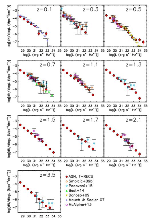
Figure 1: Comparisons between our AGN 1.4 GHz RLFs derived from the simulated catalogues (using the formalism described in Sect. 3) and observational determinations taken from literature (Padovani et al. 2015, Best et al. 2014, Donoso et al. 2009, Mauch & Sadler 2007, Smolčić et al. 2009b and McAlpine et al. 2013). The simulated sky area does not always allow sampling the highest luminosities for which we have observational determinations.

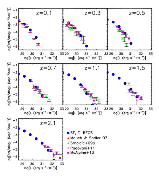
Figure 2: Comparisons between our SFG 1.4 GHz RLFs derived from the simulated catalogues (using the formalism described in Sect. 4) and observational determinations taken from literature (Padovani et al. 2011, Mauch & Sadler 2007, Smolčić et al. 2009a and McAlpine et al. 2013). The simulated sky area does not always allow sampling the highest luminosities for which we have observational determinations.

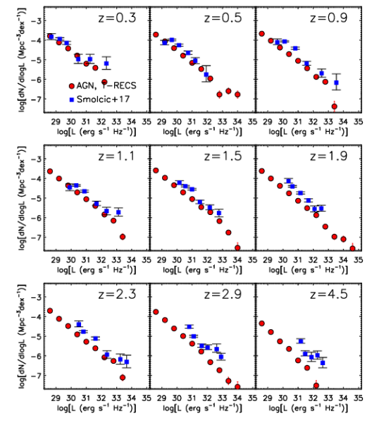
Figure 3: Comparisons between our AGN 3 GHz RLFs derived from the simulated catalogues (filled red circles) using the formalism described in Sect. 3) and the Smolčić et al. (2017c) observational determinations (filled blue squares).

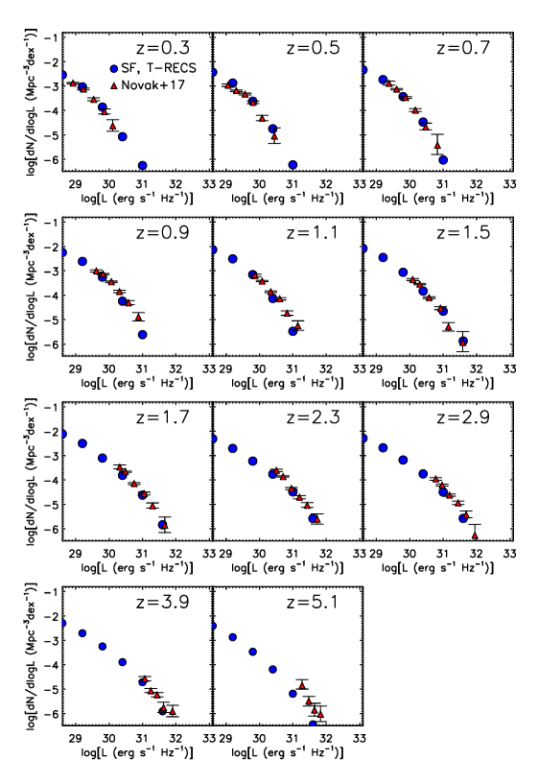
Figure 4: Comparisons between our SFG 3 GHz RLFs derived from the simulated catalogues (using the formalism described in Sect. 4) and the Novak et al. (2017) observational determinations.

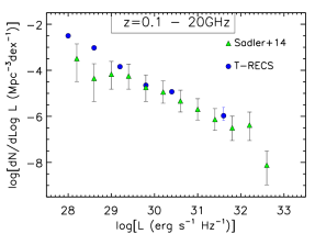
Figure 5: Comparisons between our 20 GHz RLFs of the whole (SFG+AGN) population derived from the simulated catalogues (using the formalism described in Sects. 3 and  4) and the Sadler et al. (2014) observational determinations. The simulated sky area does not allow sampling high luminosities.

3.3 Polarized intensity

We also include polarization information (in terms of the polarized intensity $P=\sqrt{Q^{2}+U^{2}}$) for each simulated source. For SS-AGNs the polarized flux densities were generated by sampling from the polarization fraction distribution at $1.4\,\mathrm{GHz}$ by Hales et al. (2014). This distribution was found to be independent of flux density down to a total intensity of $\sim$10 mJy and perhaps even of 1 mJy. In the absence of better information, we have assumed that this distribution holds at all frequencies.

In the case of flat-spectrum sources we have exploited the high sensitivity polarization measurements in seven bands (centred at 2.1, 5.5, 9, 18, 24, 33 and 38 GHz) of a complete sample of 104 compact extragalactic radio sources brighter than 200 mJy at 20 GHz, carried out by Galluzzi et al. (2018). Again, no indications of a flux-density dependence of the distribution of polarization fractions was found. Hence polarized flux densities at 5.5, 9 and 18 GHz were assigned sampling the observed distributions and interpolating at intermediate frequencies. The distribution at 1.4 GHz was computed using the polarization measurements by Condon et al. (1998) for a complete sample of 2810 flat-spectrum sources brighter than 200 mJy at 20 GHz, drawn from the Australian Telescope Compact Array 20 GHz (AT20G) survey (Murphy et al., 2010). Below 1.4 GHz the polarization fraction of each source was kept constant at the 1.4 GHz value.

We used the polarization counts resulting from those frequency-dependent polarization fractions to compute effective spectral indices in polarization for our flat-spectrum sources, with the same method described in the previous section. Consistently with that analysis, we considered again the frequency intervals 1.4–4.8 GHz and 4.8–20 GHz and a dispersion of $\sigma=0.25$. This additional step allows our polarized sources to have a regular, more physical frequency spectrum, while still being consistent with different polarization fractions at different frequencies.

3.4 Clustering

In order to assign AGN sources to underlying haloes of the base DM simulation (see Sect. 1) and recover the correct spatial correlation functions we started from Janssen et al. (2012), giving the fraction of galaxies hosting an RL AGN as a function of the host galaxy stellar mass, $M_{\star}$. Janssen et al. (2012) model the LERG and HERG populations of AGN separately. For the LERG population, the fraction is consistent with $f^{\rm LERG}\propto M_{\star}^{2.5}$, and saturates at $M_{\star}>10.^{11.6}\,M_{\odot}$; for the HERG population, the dependence is shallower ($f^{\rm HERG}\propto M_{\star}^{1.5}$).

We combined these results with the Aversa et al. (2015) relation between stellar mass and dark matter (DM) halo mass $M_{\star}=F(M_{\rm h})$ (their Table 2, including redshift evolution) to compute the probability that a halo of a given mass $M_{\rm h}$ hosts a LERG or a HERG AGN. The probability distributions that we obtain peak at $\log(M_{\rm h}/M_{\odot})=12.5$ and 12.8 for LERG and HERG respectively, with a $\sigma$ widths of 0.4 and 0.3.

We then mapped these two populations into our three observational categories:

• FSRQs from the HERG population;

• BL Lacs from the LERG population.

• SS-AGNs morphologically classified as FR II/FR I (see Sect. 3.5) from the HERG/LERG population.

We acknowledge that, while there is broad overlap between the HERG/LERG and FR I/FR II classifications, there are also differences between the two classes. For example, a significant population of FR II LERGs exists (Laing et al., 1994) and, while HERGs tend to have higher luminosities than LERGs, both HERGs and LERGs are found across the full luminosity range (e.g., Best & Heckman, 2012). However, multifrequency evolutionary models for HERGs and LERGs as advanced as those adopted here don’t exist yet. Also, clustering data on these source populations are still endowed with substantial uncertainties (cf. Hale et al., 2018, and Sect. 5.3); hence a sophisticated treatment of these populations is not warranted at this stage.

Each radio AGN in the simulated catalogue was associated to either the LERG or HERG mass distribution, as previously described, and a halo mass was drawn from it. Finally, the source was associated to the halo having the closest mass in the same redshift bin. The source was given the exact redshift and coordinates of the centre of the dark matter halo. Haloes already associated to a galaxy are excluded from the list, thus preventing multiple associations.

3.5 Source sizes

The different radio AGN populations have also different morphologies. According to the unified AGN model (e.g., Orr & Browne, 1982; Antonucci & Miller, 1985; Netzer, 1985, 1987) the compact, typically unresolved, sources (FSRQs and BL Lacs in our simulation) and the extended ones, typically exhibiting the double-lobe morphology (SS-AGNs in our simulation) are described by the same parent population, only viewed from a different angle from the jet axis.

DiPompeo et al. (2013) re-examined the unified model by fitting the distribution of intrinsic sizes of one parent population, using observational size data (e.g., Barthel, 1989; Singal & Laxmi Singh, 2013) as a constraint. We used their result as the base for our size modelling.

Depending on the population, we drew an intrinsic size from one of the distributions in DiPompeo et al. (2013, see their Table 2); sources were then given a viewing angle $\theta$ with the usual uniform distribution in $\sin(\theta)$, with different limiting angles. Specifically:

• FSRQs and BL Lacs: intrinsic size from the “empirically determined, narrow” distribution; viewing angle $0<\theta\leq 5\deg$;

• steep-spectrum AGNs: intrinsic size from the “Modelled Gaussians” distribution; viewing angle $5<\theta\leq 90\deg$.

This means that the apparent projected sizes of FSRQs and BL Lacs are small, whilst steep-spectrum AGNs may be readily resolved by survey telescopes with $\sim$ arcsecond resolution. Therefore, in our model, FR I/FR II morphologies are associated to steep-spectrum sources.

We characterise FR I and FR II by means of the $R_{s}$ parameter, defined as the ratio between the total projected source size and the projected distance between the two bright hot spots, which typically occur either side of the core emission. Fanaroff & Riley (1974) traditionally classified sources with $R_{s}>0.5$ as FR II, and with $R_{s}<0.5$ as FR I; they also gave a boundary luminosity of $P=1.3\times 10^{26}\,\hbox{W}\,\hbox{Hz}^{-1}$ at 178 MHz between the two classes, which corresponds to $L_{\rm thr,1.4\,GHz}=10^{25.4}\,\hbox{W}\hbox{Hz}^{-1}$ at 1.4 GHz (for a spectral index of $-0.8$).

Lin et al. (2010) computed the distribution of $R_{s}$ for a sample of 1040 luminous, extended radio galaxies, and found it to be bimodal, thus reflecting the FR I/FR II dichotomy. By using their $R_{s}$ distributions for the two main classes of objects, and the luminosity threshold $L_{\rm thr,1.4\,GHz}=10^{25.4}\,\hbox{W}\hbox{Hz}^{-1}$, we drew values of $R_{s}$ from a normal distribution with:

• $L_{\rm 1.4\,GHz}>10^{25.4}\,\hbox{W}\hbox{Hz}^{-1}$: mean 0.62, rms 0.18

• $L_{\rm 1.4\,GHz}<10^{25.4}\,\hbox{W}\hbox{Hz}^{-1}$: mean 0.17, rms 0.11.

Our scheme does not explicitly include the low-power, compact steep-spectrum population referred to as “FR0” sources (e.g., Sadler et al., 2014; Baldi et al., 2015, 2016). In fact, the available information on the luminosity function of these sources and on its evolution is insufficient to properly deal with them. However, the intrinsic size distribution by DiPompeo et al. (2013) in principle embraces all source populations. In particular, the adopted size distribution for low-power sources includes a substantial fraction of objects with small observed sizes. From a more general point of view, the size distribution of sources with radio luminosity in the FR0 range is anyway dominated by star-forming galaxies, hence is little affected by a somewhat imprecise modelling of the AGN radio sources.

We note that the size we model is the total core+jet emission, therefore the largest extent that the AGN would have in the sky. The brightness distribution of each source, typically very complex, means that the actually measured size could be smaller. For steep-spectrum sources, the $R_{s}$ parameter can be used to scale the total size to that containing most of the brightness (the core and the hot spots). Flat-spectrum sources are typically core-dominated, and are typically not resolved even with sub-arcsecond VLBI observations.

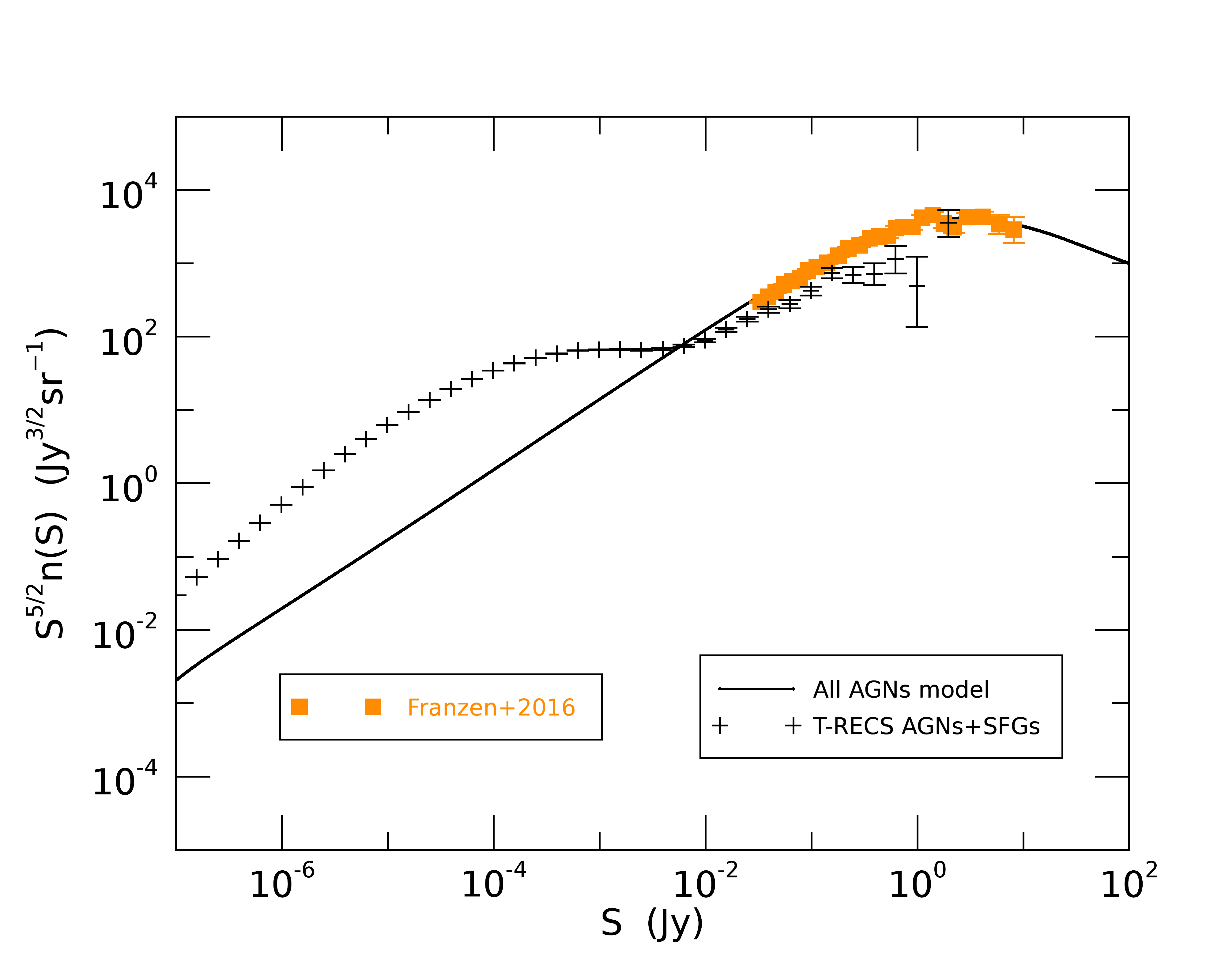
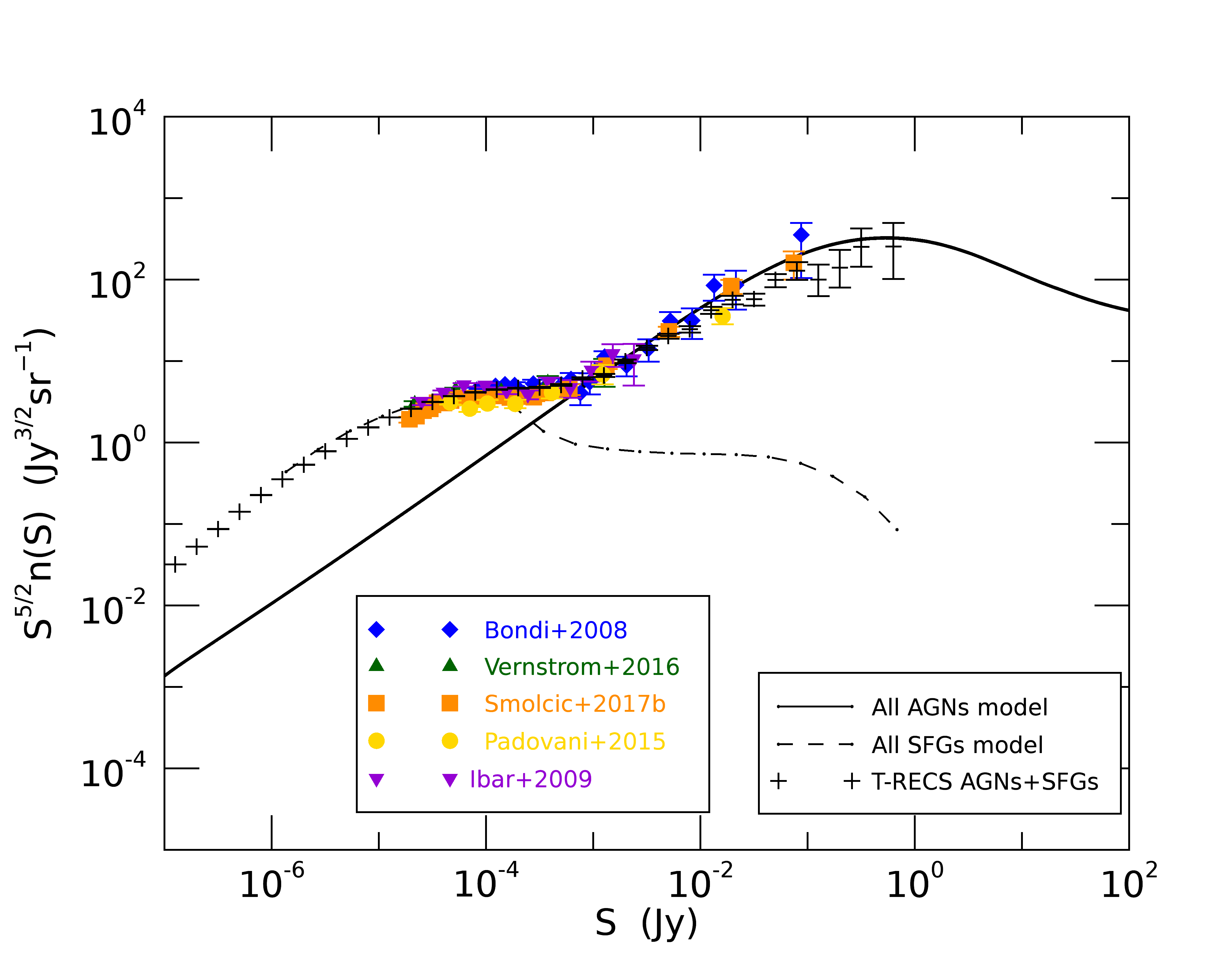
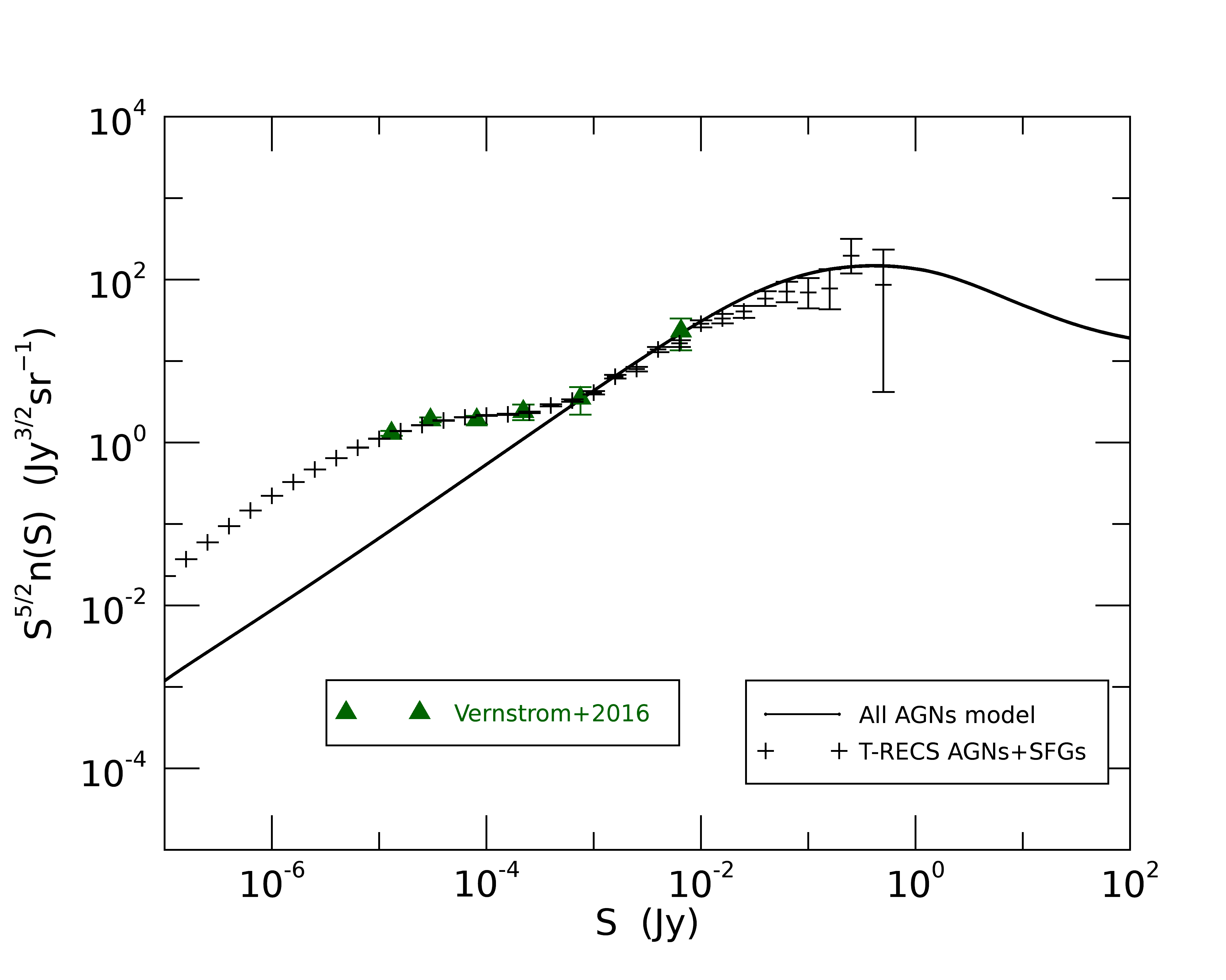
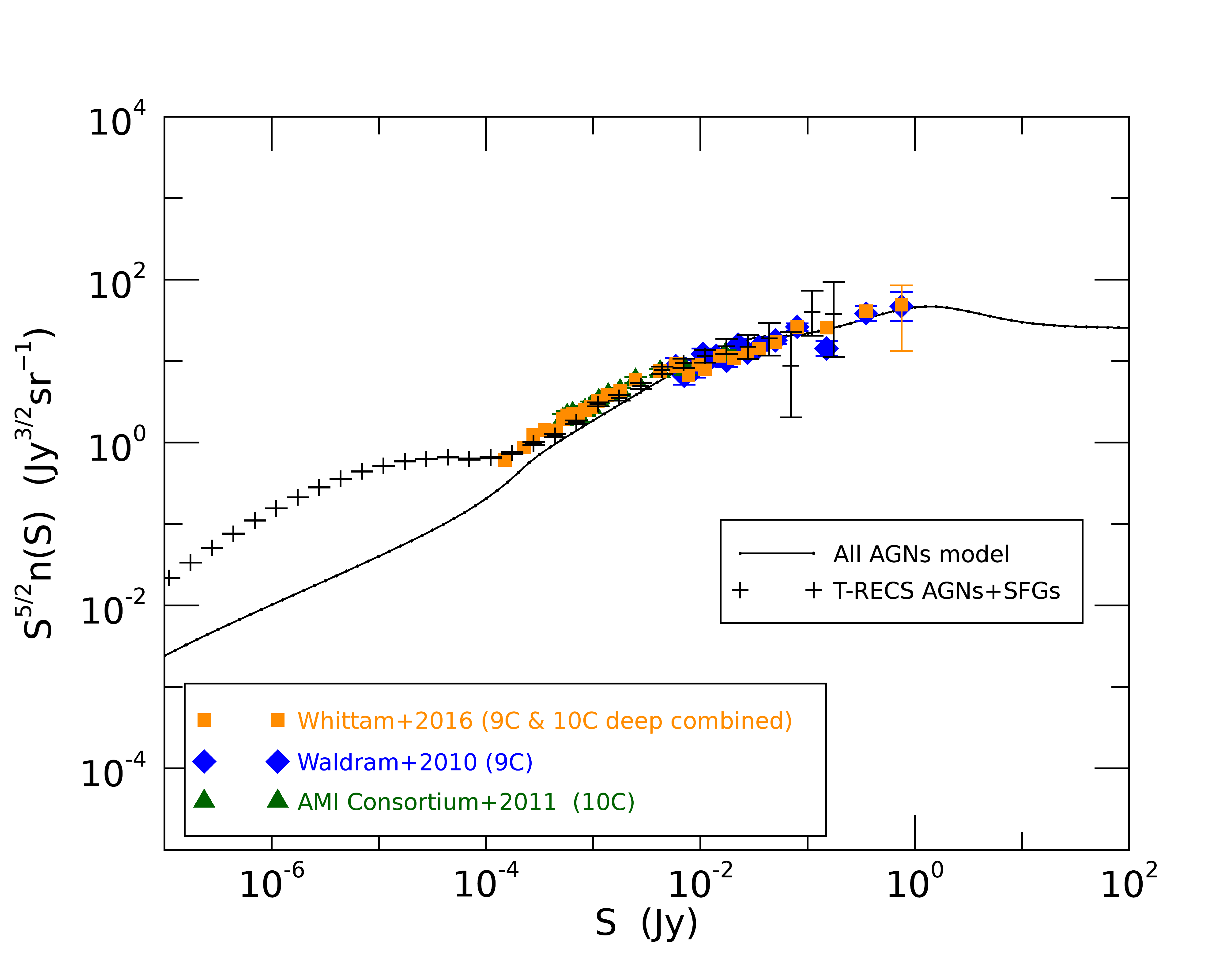
Figure 6: Comparison of differential source counts in total intensity at 150 MHz (top left) 1.4 GHz (top right), 3 GHz (bottom left) and 15 GHz (bottom right) between T-RECS, models from Bonato et al. (2017) and the available data from Franzen et al. (2016); Bondi et al. (2008); Vernstrom et al. (2016); Smolčić et al. (2017b); Padovani et al. (2015); Ibar et al. (2009); Whittam et al. (2016); Waldram et al. (2010); AMI Consortium et al. (2011).

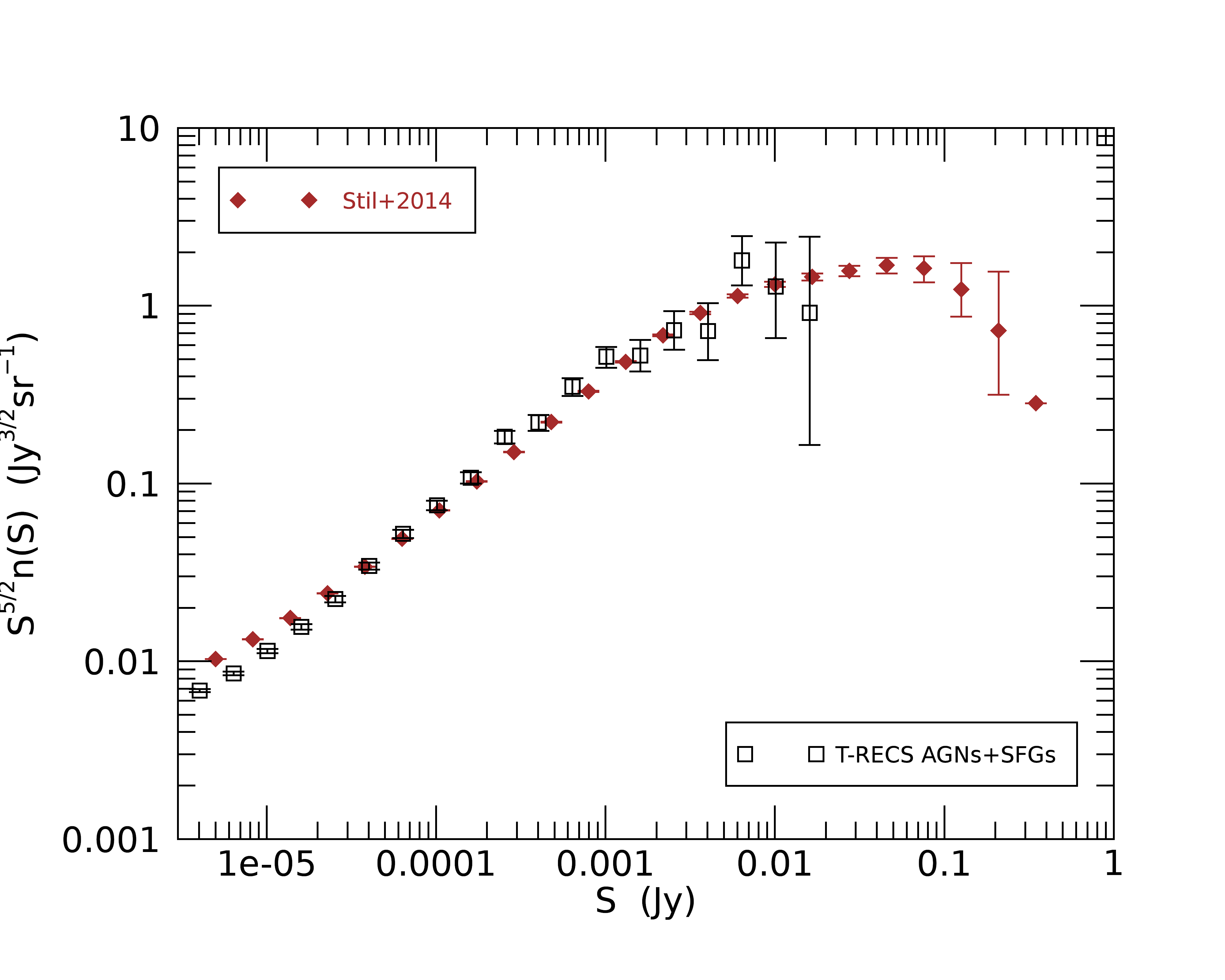
Figure 7: Comparison of polarization differential source counts from T-RECS with those estimated by Stil et al. (2014)

4 Star-forming galaxies model description

4.1 Base evolutionary model

The radio continuum emission of SFGs is tightly correlated with the star formation rate (SFR; e.g. Kennicutt & Evans, 2012, and references therein); hence the redshift-dependent radio luminosity function of SFGs can be derived from the evolving SFR function. A detailed study of the evolution of the SFR function across the cosmic time was carried out by Cai et al. (2013) focussing on IR data and by Cai et al. (2014) at $z\mathrel{\hbox to0.0pt{\lower 3.0pt\hbox{$\sim$}\hss}\raise 2.0pt\hbox{$>$}}2$ focussing on UV and Ly$\alpha$ data but taking into account also dust attenuation and re-emission. The model was extended by Mancuso et al. (2015) and further successfully tested against observational determinations of the H$\alpha$ luminosity function at several redshifts. On the whole, data useful to derive the SFR function over substantial SFR intervals are available up to $z\simeq 6$–7, with some information extending up to $z\sim 10$ (see also Aversa et al., 2015). The combination of dust extinction corrected UV/Ly$\alpha$/H$\alpha$ data with FIR data yielded accurate determinations of the SFR function over such redshift range.

The Cai et al. (2013) model also yields estimates of the effect of strong gravitational lensing on the observed LFs of high-$z$ SFGs. We have exploited it to take into account, in the simulations, strongly lensed (magnification $\mu\geq 2$) galaxies. Although the contribution of these objects to the number counts is small, they are a substantial fraction of the highest redshift galaxies that should be detected by radio surveys at few $\mu$Jy/sub-$\mu$Jy levels (Mancuso et al., 2015).

The radio continuum emission of SFGs consists of a nearly flat-spectrum free-free emission plus a steeper-spectrum synchrotron component. A calibration of the relations between SFR and both emission components was derived by Murphy et al. (2011) and Murphy et al. (2012). Following Mancuso et al. (2015) we have rewritten such relations as follows:

$$L_{\rm ff}(\nu) = 3.75\times 10^{19}\frac{\hbox{SFR}}{M_{\odot}/\hbox{yr}}\,\left(\frac{T}{10^{4}\,\hbox{K}}\right)^{0.3}$$ (8)

$$\cdot \hbox{g}(\nu,\hbox{T})\,\exp{\left(-{h\nu\over k\hbox{T}}\right)}\ \hbox{W}\,\hbox{Hz}^{-1},$$

where $T$ is the temperature of the emitting plasma (we have set $T=10^{4}\,K$) and $\hbox{g}(\nu,\hbox{T})$ is the Gaunt factor;

$$\bar{L}_{\rm sync} \simeq 1.9\times 10^{21}\left(\frac{\hbox{SFR}}{\hbox{M}_{\odot}\hbox{yr}^{-1}}\right)\left(\frac{\nu}{\hbox{GHz}}\right)^{-0.85}$$ (9)

$$\cdot \left[1+\left({\nu\over 20\rm GHz}\right)^{0.5}\right]^{-1}\,\hbox{W}\,\hbox{Hz}^{-1}.$$

However, Mancuso et al. (2015) showed that this relation, combined with observational determinations of the local SFR function, leads to an over-prediction of the faint end of the local radio LF of SFGs worked out by Mauch & Sadler (2007). A similar conclusion was previously reached by Massardi et al. (2010).

Consistency with the Mauch & Sadler (2007) LF was recovered assuming that the radio emission from low-luminosity galaxies is substantially suppressed, compared to brighter galaxies. Following Mancuso et al. (2015) we adopt a deviation from a linear $L_{\rm sync}$–SFR relation described by:

$$L_{\rm sync}(\nu)=\frac{L_{\star,\rm sync}(\nu)}{\left({L_{\star,\rm sync}}/{\bar{L}_{\rm sync}}\right)^{\beta}+\left({L_{\star,\rm sync}}/{\bar{L}_{\rm sync}}\right)},$$ (10)

where $L_{\star,\rm sync}=0.886\,\bar{L}_{\rm sync}({\rm SFR}=1\,M_{\odot}\,\hbox{yr}^{-1})$ with $\bar{L}_{\rm sync}$ given by eq. (9), and $\beta=3$; at 1.4 GHz, $L_{\star,\rm sync}\simeq 10^{28}\,\hbox{erg}\,\hbox{s}^{-1}$ $\hbox{Hz}^{-1}$. Again following Mancuso et al. (2015) we allow for a dispersion $\sigma_{\log L}=0.4$ around the mean ${L}_{\rm sync}$–SFR relation.

4.2 Total intensity number counts

For our simulations, we sampled the redshift-dependent SFR functions by Mancuso et al. (2015) and converted each galaxy’s SFR to a total radio emission in the 150 MHz–20 GHz frequency range by taking into account synchrotron, free-free, and thermal dust emission, as detailed in the following.

For free-free and synchrotron emission we use eqs. (8) and (10), respectively. Recent investigations (Magnelli et al., 2015; Delhaize et al., 2017) have reported evidence of a weak but statistically significant increase with redshift of the ratio between synchrotron luminosity and far-infrared luminosity, generally believed to be a reliable measure of the SFR, at least for $L_{\rm sync}\gg L_{\star,\rm sync}$ (although the radio excess at high $z$ might be due to residual AGN contributions; Molnár et al., 2018). We have allowed for the corresponding evolution of the mean ${L}_{\rm sync}$–SFR relation adopting:

$$\log L_{\rm synch,1.4\,\rm GHz}(z) = \log L_{\rm synch,1.4\,\rm GHz}(0)$$ (11)

$$+ 2.35[1-(1+z)^{-0.12}].$$

Bonato et al. (2017) showed that this relation, based on the results of Magnelli et al. (2015), yields a very good fit of the observational estimates of the radio luminosity function of SFGs, recently determined up to $z\simeq 5$ (Novak et al., 2017) as well as of the ultra-deep source counts at 1.4 GHz (Vernstrom et al., 2014, 2016; Smolčić et al., 2017b).

As illustrated by Fig. 5 of Mancuso et al. (2015), the rest-frame spectral energy distribution (SED) of SFGs at $\nu\mathrel{\hbox to0.0pt{\lower 3.0pt\hbox{$\sim$}\hss}\raise 2.0pt\hbox{$>$}}100\,$GHz is dominated by thermal dust emission. This implies that, in the case of high-$z$ galaxies, this component becomes important already at frequencies of a few tens of GHz in the observer’s frame. We have taken it into account using the Cai et al. (2013) model.

The model comprises three SFG populations with different evolutionary properties and different dust emission SEDs: ‘warm’ and ‘cold’ late-type galaxies, and proto-spheroids. In the simulations, we have used the calibration adopted by Cai et al. (2013) to translate its SFR into its total infrared (IR; 8–1000 $\mu$m) luminosity, $L_{\rm IR}$:

$$\log(L_{\rm IR}/L_{\odot})=\log(\hbox{SFR}/M_{\odot}\,\hbox{yr}^{-1})+9.892.$$ (12)

The monochromatic luminosity of dust emission at the frequency $\nu$, $L_{\rm dust}(\nu)$, was obtained from $L_{\rm IR}$ using the SED appropriate for each population, given by Cai et al. (2013), and added to the radio luminosity.

4.3 Polarized intensity

The polarization properties of star-forming galaxies are still poorly known. The polarized signal is typically only a few percent of the total brightness, but it depends strongly on frequency and on galaxy inclination, due to depolarization effects. All these features are captured by Sun & Reich (2012), which study the polarization properties of Milky-Way-like galaxies with a three-dimensional emission model. They derive polarization percentages as a function of galaxy inclination for 5 frequencies: 1.4, 2.7, 4.8, 8.4 and 22 GHz (see their Fig. 9). We model each curve with a fourth-order polynomial, which we use to compute the polarization percentage at all 5 frequencies for a randomly generated galaxy inclination $i$ (with a uniform distribution in $\sin(i)$). This yields median polarization fractions of $\sim$4.2 % at 4.8 GHz and $\sim$0.8 % at 1.4 GHz, which are consistent with other observations (Stil et al., 2009; Taylor et al., 2014). We then interpolate linearly the polarization percentages for any other frequency. We finally obtain a polarization spectrum by multiplying the frequency-dependent polarization fraction by the total intensity spectrum. We used the interpolated polarization fraction values for each galaxy directly, without drawing them from a random distribution, to ensure that the resulting polarized spectrum is smooth in frequency. Differences in the spectra of individual sources are anyway obtained thanks to the dependence of polarization fractions on random inclinations and by the scatter in the total intensity spectral indices.

4.4 Clustering

In order to populate our simulated DM haloes (see Sect. 1) with radio-emitting SFGs we use an abundance matching procedure (e.g. Moster et al., 2013). Abundance matching is a method to constrain a relationship between two quantities (in our case, radio luminosity $L$ and halo mass $M_{\rm h}$) whose individual distributions are known (radio luminosity function and dark halo mass function).

We used the $L_{\rm SFR}$–$M_{\rm h}$ relation from Aversa et al. (2015), which is of the form:

$$L(M_{\rm h})=N\times\Big{[}\Big{(}\frac{M_{\rm h}}{M_{b}}\Big{)}^{\alpha}+\Big{(}\frac{M_{\rm h}}{M_{b}}\Big{)}^{\omega}\Big{]}^{-1},$$ (13)

where $N$, $\alpha$, $\omega$ and $M_{b}$ are free parameters which include redshift evolution. We fitted for them separately for each redshift slice, by requiring that the luminosity function derived from the mass function of the cosmological simulation through eq. (13) matched as closely as possible the radio luminosity function at 1.4 GHz from Bonato et al. (2017).

By inverting the best-fit $L(M_{\rm h})$ relation, we finally map radio luminosities into halo masses for each redshift slice. This allows us to associate galaxies to haloes in the light cone. Once a galaxy is associated to a halo, we assign to it the redshift and the sky coordinates of the centre of the halo.

As stated in Sect. 2, the minimum halo mass of the simulation is $M_{\rm h,min}=1.061\times 10^{8}\,h^{-1}\,M_{\odot}$, which sets the minimum luminosity of galaxies that we can associate to haloes with this method to $L_{\rm min,1.4GHz}\simeq 10^{22}$ erg/s/Hz, depending on the redshift. For less luminous galaxies, we assume a random distribution in the sky.

4.5 Source sizes

For SFG sizes we make reference to the scale radius $r_{0}$ of an exponential emission intensity profile:

$$I(r)=I_{0}\exp(-r/r_{0}).$$ (14)

Shen et al. (2003) have given a relation between the optical half-light radius of disk galaxies, $R$, and their stellar mass:

$$R({\rm kpc})=\gamma M_{\star}^{\alpha}(1+M_{\star}/M_{0})^{\beta-\alpha},$$ (15)

where $\alpha$, $\beta$, $\gamma$ and $M_{0}$ are free parameters. We have performed a new fit for these parameters to match a set of radio observations: those of Biggs & Ivison (2006), Owen & Morrison (2008) and Schinnerer et al. (2010). These three papers give galaxy sizes defined as the FWHM of a Gaussian intensity profile: we derived the scale radius as $r_{0}=0.7\,r_{\rm FWHM}$. We performed a joint fit to all three size distributions, finding the following values of the parameters: $\alpha=0.115$, $\beta=0.898$, $\gamma=0.199$, $M_{0}=3.016\cdot 10^{10}M_{\rm sun}$.

For each source, we first computed the stellar mass $M_{\star}$ from the halo mass $M_{\rm h}$ using the $M_{\star}$–$M_{\rm h}$ relation by Aversa et al. (2015), with the parameter values listed in their Table 2. We then computed the scale radius with eq. (15) with our values for $\alpha$, $\beta$, $\gamma$ and $M_{0}$. We allowed for a dispersion of $\sigma_{\rm lnR}=\sigma_{2}+(\sigma_{1}-\sigma_{2})/[1+(M_{*}/M_{0})^{2}]$, with $\sigma_{1}=0.47$ and $\sigma_{2}=0.34$ as in Shen et al. (2003). Finally, the physical size was converted into an apparent one, depending on the redshift.

Galaxy ellipticity for our galaxies was generated in terms of the $(e1,e2)$ components along the two main axes of the field of view. For the absolute value of the ellipticity we used the distribution

$$P(|e|)=|e|\left[\cos(\frac{\pi|e|}{2})\right]^{2}\exp\left[-\frac{2|e|}{B}\right]^{C}$$ (16)

with $B=0.19$ and $C=0.58$, as derived by Tunbridge et al. (2016) performing shape measurements on Very Large Array (VLA) Cosmological Evolution Survey (COSMOS) radio data. We then generated random orientation angles $0\leq\theta\leq 2\pi$ and projected the absolute ellipticity into the two components with:

$$e1 = |e|\sin(\theta/2)$$ (17)

$$e2 = |e|\cos(\theta/2).$$ (18)

5 Validation

This section presents comparisons between the outputs of the T-RECS simulation and the available real data.

5.1 Luminosity functions

Figures 1 and  2 compare the 1.4 GHz Radio Luminosity Functions (RLFs) of radio AGNs and SFGs, respectively, derived from the simulated catalogues, with the observational determinations at several redshifts available in the literature. The simulated catalogues were obtained using the formalisms described in Sects. 3 and  4. For both populations, the figures show a very good agreement between our simulated RLFs and literature data.

In Fig. 3 the 3 GHz AGN RLFs derived from our simulated catalogues are compared with the recent Smolčić et al. (2017c) observational estimates derived from VLA-COSMOS. Note that, although the survey was carried out at 3 GHz, Smolčić et al. (2017c) presented RLFs converted to 1.4 GHz. The conversion was made using the measured spectral indices for sources ($\sim 50\%$ of the sample) detected also at 1.4 GHz. For the remaining $\sim 50\%$ of the sample a constant spectral index $\alpha=-0.7$ was adopted.

We converted the Smolčić et al. (2017c) RLFs back to 3 GHz using $\alpha=-0.7$. Our simulated RLFs are consistent with these observational estimations up to $z\sim 1.0$. At higher redshifts our RLFs are a factor of $\sim 3$-5 lower. This discrepancy may be due to the fact that the Smolčić et al. (2017c) radio AGN population includes galaxies hosting AGNs, irrespective of their radio emission. “Radio quiet” AGNs are their dominant AGN sub-population at $z\gtrsim 1.2$ (see their Fig. 7). According to the adopted model, the radio emission of these objects is generally dominated by star formation in the host galaxies. Therefore they are included in the SFG population. Moreover the high$-$z Smolčić et al. (2017c) RLFs are significantly higher than the previous observational determinations (see their Fig. 3).

Figure 4 compares our 3 GHz SFG RLFs with the recent observational estimates by Novak et al. (2017), again derived from the 3 GHz VLA-COSMOS survey. Also in this case we converted the Novak et al. (2017) RLFs, tabulated at 1.4 GHz in their paper, to 3 GHz using a spectral index $\alpha=-0.7$, as done by Novak et al. (2017) to make the opposite conversion (for 75% of their sources). The agreement with these observational results is very good. Note that the space densities of SFGs are generally substantially higher than those of radio AGNs, so that the contribution of radio quiet AGNs, present in our RLFs but not in those by Novak et al. (2017), does not make a substantial difference.

Finally, in Fig. 5, we compare our simulated 20 GHz RLFs of the whole (AGN+SFG) population with the local Sadler et al. (2014) estimation. Our results are consistent (within the error bars) with these data, apart at the lowest radio luminosities shown in the figure, where the Sadler et al. (2014) RLFs may be affected by incompleteness.

5.2 Differential source counts

Figure 6 presents the comparison between T-RECS differential source counts in total intensity at 150 MHz, 1.4 GHz 3 GHz and 15 GHz and with the available data (Franzen et al., 2016; Bondi et al., 2008; Vernstrom et al., 2016; Smolčić et al., 2017b; Padovani et al., 2015; Whittam et al., 2016; Waldram et al., 2010; AMI Consortium et al., 2011; Ibar et al., 2009). We also checked the agreement at 20 GHz with the AT20G (Murphy et al., 2010) and at 610 MHz with GMRT observations (Garn et al., 2008). Note that the simulated area ($5\times 5\,\hbox{deg}^{2}$) is too small to adequately sample sources brighter than a few hundred mJy at 1.4 GHz. The shape of the counts yielded by our model is shown by the solid lines in Fig. 6. The total counts agree very well with the available data, both in the regime dominated by RL AGNs and in the one dominated by SFGs and RQ AGNs. We note the much closer agreement at 1.4 GHz in the sub-mJy regime of our simulation with respect to Wilman et al. (2008), whose counts were around a factor 2 lower (Bonaldi et al., 2016). We also note that the good agreement persists over the whole frequency range explored, thus confirming the validity of the approaches used to associate frequency spectra to the sources, described in Sect. 3 and 4.

Figure 7 compares our polarization counts at 1.4 GHz with the results from Stil et al. (2014). The counts were obtained from total intensity source counts after assuming a polarization fraction distribution obtained from NRAO VLA Sky Survey (NVSS) data. This analysis is therefore quite similar to what we have adopted for our simulation. Since our simulation in total intensity is consistent with the 1.4 GHz data and the polarization fraction estimates from Stil et al. (2014) are similar to those from Hales et al. (2014), the agreement of our results with Stil et al. (2014) is not surprising.

5.3 Clustering

Observational estimates of the 2-point angular correlation function, $w(\theta)$, of both radio AGNs and SFGs have been recently obtained by Magliocchetti et al. (2017) and Hale et al. (2018).

Magliocchetti et al. (2017) investigated the clustering properties of a complete sample of 968 radio sources brighter than 0.15 mJy at 1.4 GHz, detected by the VLA on the COSMOS field covering about $2\,\hbox{deg}^{2}$. Spectroscopic redshifts are available for 52% of the sources and photometric redshifts for a further 40%. Sources with redshift determinations were subdivided into radio AGNs (644 objects) and SFGs (247 objects) purely on the basis of their radio luminosity. In practice, all sources with luminosity below/above a suitably chosen redshift-dependent threshold were classified as SFGs/AGNs.

The top panel Fig. 8 shows that the global redshift distribution of simulated sources is consistent with the observational estimate, not surprisingly since the simulation reproduces reasonably well both the 1.4 GHz counts (Fig. 6) and the redshift-dependent luminosity functions of both the radio AGNs (Fig. 1) and the SFGs (Fig. 2). Note that the true uncertainties of the observational determination are substantially larger than the Poisson fluctuations because of the contributions of the errors on photometric redshifts and of the sample variance.

As illustrated by the lower panels of Fig. 8, there are pronounced differences between the simulation and the estimates for each population. Most of the difference is due to their selection of SFGs. For example, at $z=0.7$ they set the boundary between SFGs and radio AGNs at $\log(L_{1.4\rm GHz}/\hbox{erg}\,\hbox{s}^{-1}\,\hbox{Hz}^{-1})=30.5$, but the observed radio luminosity function of SFGs at this $z$ extends up to $\log(L_{1.4\,\rm GHz})\sim 31.8$ (see Fig. 2); at $z=1.5$ the boundary is at $\log(L_{1.4\,\rm GHz})\sim 31.3$ with the luminosity function reaching $\log(L_{1.4\,\rm GHz})\sim 32.2$, and so on. Thus the Magliocchetti et al. (2017) criterion misses the brightest SFGs, especially around $z\sim 1$, where their redshift distribution has an unnatural minimum. The missed SFGs are classified as radio AGNs, resulting in the excess over the simulation around $z\sim 1$. This difference in the source classification between T-RECS and Magliocchetti et al. (2017) needs to be taken into account when comparing the correlation functions.

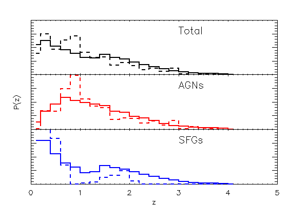
Figure 8: Redshift distributions of Magliocchetti et al. (2017) (dashed lines) compared with our catalogue for the same flux cut and sky area (solid lines).

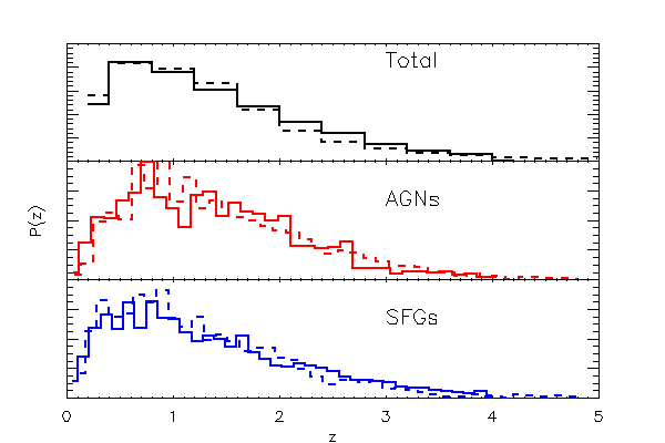
Figure 9: Redshift distribution of the total sample of Hale et al. (2018) (dashed line) compared with our catalogue for the same flux cut and sky area (solid line).

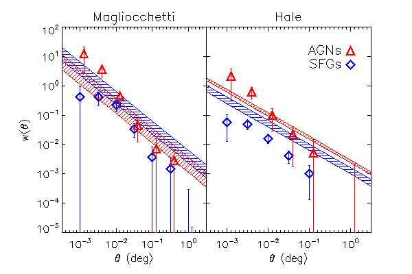
Figure 10: Two-point angular correlation function $w(\theta)$ yielded by our simulation for radio AGNs and SFGs (points with error bars) compared to the results of Magliocchetti et al. 2017 (left) and Hale et al. 2018 (right) for the same populations (shaded areas represent the best fit $\pm 1\,\sigma$ uncertainty in the normalization).

The broad minimum in the simulated redshift distribution of SFGs between $z=1$ and $z=1.2$ corresponds to the transition between the dominance of late-type galaxies, that are the main star forming population at $z\leq 1$, and proto-spheroidal galaxies that take over at higher $z$. This transition is in keeping with data on the age of stellar populations of the two galaxy types (e.g., Bernardi et al., 2010)

Hale et al. (2018) measured $w(\theta)$ for the recently released, deeper 3 GHz VLA/COSMOS sample. They used a $5.5\,\sigma$ cut on the final catalogue, corresponding to a mean flux density limit of $S_{3\,\rm GHz}\simeq 13\,\mu\hbox{Jy}\,\hbox{beam}^{-1}$ or of $S_{1.4\,\rm GHz}\simeq 22\,\mu\hbox{Jy}\,\hbox{beam}^{-1}$ for $S\propto\nu^{-0.7}$. Their catalogue contains a total of 8928 sources over $\sim 2\,\hbox{deg}^{2}$.

The source identification was made by Smolčić et al. (2017a) by cross-matching with optical, near-infrared, mid-infrared (Spitzer/IRAC) and X-ray data.

Optical counterparts to $\sim 86\%$ of the $\geq 5.5\,\sigma$ radio sources were found, and for 98% of them photometric or spectroscopic redshifts were gathered. About 79% of the sources were further classified as SFGs or AGNs, based on various criteria, such as X-ray luminosity; observed mid-infrared color; UV/far-infrared spectral energy distribution; rest-frame, near-UV optical colour corrected for dust extinction; and radio excess relative to that expected from the star formation rate of the hosts.

In interpreting the Hale et al. (2018) results, it should also be taken into account that the presence of an active nucleus detected via its IR/optical/UV/X-ray emission does not necessarily imply that it gives a significant contribution to the radio emission.

Figure 9 compares the redshift distributions from Hale et al. (2018) to those from our simulation, for the same flux density limit and sky area. The agreement is very good both on the total population and the AGN and SFG populations separately, thus indicating that source classification in this case is more consistent, which allows an easier comparison of the correlation functions as well.

Figure 10 compares the 2-point angular correlation function, $w(\theta)$, for our AGNs and SFGs catalogues with those from Magliocchetti et al. (2017) and from Hale et al. (2018). Both observational estimates adopted the standard power-law shape for the correlation function: $w(\theta)=A\theta^{1-\gamma}$. Since the data did not allow an accurate determination of both $A$ and $\gamma$ for each source population, they fix $\gamma$ to 2 and 1.8, respectively, and fit for the normalization. As they point out, this implies that the errors on $w(\theta)$ are underestimated.

To produce the T-RECS correlation functions, we used the full $5\times 5$ deg² sky area and the same flux limits of the observational estimates. We used the Hamilton (1993) estimator:

$$w(\theta)=\frac{DD\cdot RR}{DR\cdot DR}-1,$$ (19)

where $DD$, $RR$ and $DR$ are the number of data-data, random-random and data-random pairs separated by $\theta$.

The random catalogue has been constructed redistributing uniformly the simulated sources between -2.5 and 2.5 degrees from the center of the patch, both in longitude and in latitude. The $w(\theta)$ was computed for 100 realizations. In Fig. 10 we show the mean values and their dispersions as a function of the angular scale.

We find that, for T-RECS, implementation details on how galaxies of a modelled halo mass $M_{\rm h}$ are associated to the actual haloes of the cosmological simulation have a non-negligible effect on the measured $w(\theta)$. The mass function of the cosmological simulation and that inferred from the luminosity function are somewhat different, which means that there is a deficit of suitable haloes in some mass ranges and a surplus in others. Allowing for some scatter between the predicted and the associated mass (as done for the results shown in Fig. 10) alleviates the problem, however it typically favours association to smaller halo masses, given the shape of the mass function.

Our simulations give amplitudes of the angular correlation function of SFGs consistently lower than those of both Magliocchetti et al. (2017) and Hale et al. (2018). The discrepancies are of 1.7 $\sigma$ and 2.5 $\sigma$ respectively, where $\sigma$ is the quadratic sum of errors of the observational estimates and of the simulations. The higher amplitudes of the observationally estimated $w(\theta)$ imply higher average bias factors, i.e. higher halo masses.

The halo masses inferred by Magliocchetti et al. (2017) are far higher than those corresponding to their average stellar masses given by the halo to stellar mass relations by Moster et al. (2010). According to these relations the minimum halo mass of SFGs ($\log(M_{\rm min}/M_{\odot})=13.1$) corresponds, at their average redshift ($\langle z\rangle=0.5$), to a minimum stellar mass of $\log(M_{\rm min}/M_{\odot})=11.2$. But their average stellar mass is $\log\langle M_{\star}/M_{\odot}\rangle=10.7\pm 0.5$, corresponding to an average halo mass of $\log(M_{\rm h}/M_{\odot})\simeq 12.3$.

Looking at that the other way round, for the Magliocchetti et al. (2017) flux cut the halo mass distribution of SFGs resulting from the T-RECS simulation peaks at $\log(M_{\rm h}/M_{\odot})=12.5$, only slightly higher than the average halo mass corresponding to their average stellar mass. This small excess was indeed expected since, as argued above, Magliocchetti et al. (2017) somewhat underestimated the fraction of high-$z$ SFGs, hence their mean stellar mass.

The fact that the simulations yield halo mass distributions of SFGs consistent with the stellar mass distributions derived by Magliocchetti et al. (2017), but falls short of their estimates of the angular correlation function may suggest that the latter is anomalously high. Hale et al. (2018) do not give estimates of stellar masses; hence the same test cannot be done. However, none of our simulations gives an amplitude of $w(\theta)$ as large as that observationally estimated, suggesting that part of the discrepancy can be due to the issue, discussed above, of the association between galaxies and simulated haloes introducing some scatter in mass.

The amplitudes of the AGN correlation functions from our simulations are consistent, on average, with the observational estimates by both Magliocchetti et al. (2017) and Hale et al. (2018), but the slope is somewhat steeper. We remind, however, that in both cases the data were not sufficient to simultaneously determine the amplitude and the slope of the $w(\theta)$; hence $\gamma$ was not measured but was fixed at 2 and 1.8, respectively.

According to the simulations, the halo mass distribution of radio AGNs at the Magliocchetti et al. (2017) flux density limit peaks at $\log(M_{\rm h}/M_{\odot})=12.5$. At the mean redshift of 1.25 this corresponds to $\log(M_{\star}/M_{\odot})=10.7$, in good agreement with the average stellar mass reported by Magliocchetti et al. (2017): $\log\langle M_{\star}/M_{\odot}\rangle=10.9\pm 0.5$.

Despite the differences noted above, and taking into account the uncertainties in both determinations, the agreement between the T-RECS clustering and the empirically-determined one is reasonably good.

5.4 Source sizes

In Fig.11 we compare the median source size as a function of 1.4 GHz flux density from T-RECS with the literature.

The size of AGNs does not depend on the flux density. As explained in Sec.3.5, flat-spectrum (FS) sources (FSRQ and BLLac in our model) have been associated to small view angles and therefore to compact, beamed objects, while SS sources have been associated to larger view angles and FRI/FRII morphologies. This results in a marked difference (more than two orders of magnitude) between the size of flat and steep-spectrum AGNs. We find good agreement between T-RECS and observations (Coleman & Condon, 1985; Kapahi et al., 1987) on the size of SS AGNs.

The size of SFGs increase with increasing flux, through the dependence of both quantities on the source redshift. To compare our results with the literature (Biggs & Ivison, 2006; Owen & Morrison, 2008; Schinnerer et al., 2010; Cotton et al., 2018), we show in Fig.11 the median size at the median flux density of each observed sample, multiplied by 0.7 to convert from the Gaussian FWHM of the observational determinations to the exponential scale radius of our simulation. Overall there is a good agreement between T-RECS sizes and observed sizes.

The median size of the sample including all T-RECS sources (labelled “total” in Fig. 11) has a complex dependence on flux density, due to the fact that different populations dominate the total counts at different fluxes. At flux densities over $\sim$1 mJy, the median size closely follows that of AGNs and it is therefore quite flat; at lower flux densities, the behaviour is that of SFGs and it is much steeper.

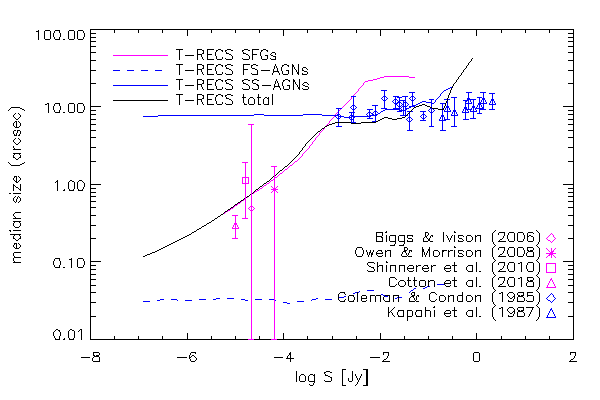
Figure 11: Median sizes as a function of 1.4 GHz flux for T-RECS (lines) and data from the literature (Schinnerer et al., 2010; Biggs & Ivison, 2006; Owen & Morrison, 2008; Kapahi et al., 1987; Coleman & Condon, 1985; Cotton et al., 2018, symbols with error bars).

6 Available products

We release catalogues generated with the T-RECS code organised in three tiers:

1. deep: 1 deg² 1.4 GHz flux limit 1 nJy, data size 820 Mb

2. medium: 25 deg², 1.4 GHz flux limit 10 nJy data size 6 Gb

3. wide: 400 deg², 1.4 GHz flux limit 100 nJy, no clustering, data size 32 Gb

The format and the content of each catalogue is described in Appendix A. The frequencies at which we provide total intensity and polarization flux densities are listed in Table 2. They have been chosen to span the whole simulated 150 MHz–20 GHz frequency range, to be typically spaced by $\sim$ 30 % fractional bandwidth, and to include the frequencies allowing comparison with other data in Figures 1–7.

Table 2: Frequencies in the T-RECS released catalogues

Frequency	SKA bands	Data
150 MHz	Low	(1)
160 MHz	Low
220 MHz	Low
300 MHz	Low
410 MHz	Mid Band1
560 MHz	Mid Band1
780 MHz	Mid Band1
1.0 GHz	Mid Band2
1.4 GHz	Mid Band2	(2) (3) (4) (5) (7)
1.9 GHz	Mid Band3
2.7 GHz	Mid Band3
3.0 GHz	Mid Band4	(3)
3.6 GHz	Mid Band4
5.0 GHz	Mid Band5a
6.7 GHz	Mid Band5a
9.2 GHz	Mid Band5b
12.5 GHz	Mid Band5b
20.0 GHz		(6)

¹Franzen et al. (2016)
²Bondi et al. (2008)
³Vernstrom et al. (2016)
⁴Smolcic et al. (2017)
⁵Padovani et al. (2015)
⁶Sadler et al. (2014)
⁷Ibar et al. (2009)

More catalogues can be generated with different specifications if needed, by either requesting them or by running the T-RECS code to produce them.

Table 3 gives, as an example, the integral source counts at 3 frequencies (150 MHz, 1.4 GHz and 20 GHz) computed from the 25 deg² catalogue, which can be used to predict how many sources can be detected for a given flux density limit and source population. These numbers do not take into account the effect of PSF, noise or confusion, therefore they represent an ideal case.

Table 3: Integral source counts $\log N(>S)$ at 150 MHz, 1.4 GHz and 20 GHz computed from the 25 deg² T-RECS catalogue, for all the modelled populations and sub-populations (identified by the numbers 1,2,3 for late-type, spheroidal and lensed spheroidal SFGs; 4,5,6 for FSRQ, BLLac and SS-AGNs).

150 MHz
$\log S$ [Jy]	$\log N(>S)$
	Total	Tot AGNs	AGN (4)	AGN (5)	AGN (6)	Tot SFGs	SFG (1)	SFG (2)	SFG (3)
0.50	2.72	2.72			2.72
0.00	3.39	3.39	2.11		3.37
-0.50	3.90	3.88	2.81		3.85	2.41	2.41
-1.00	4.39	4.37	3.11	2.11	4.34	3.15	3.15
-1.50	4.81	4.77	3.63	2.72	4.73	3.75	3.74	2.11
-2.00	5.25	5.14	4.04	3.11	5.10	4.62	4.56	3.72	2.41
-2.50	5.82	5.47	4.45	3.63	5.42	5.57	5.43	5.01	3.39
-3.00	6.52	5.77	4.83	4.17	5.70	6.44	6.25	5.98	4.10
-3.50	7.19	6.06	5.21	4.58	5.98	7.15	6.97	6.69	4.71
-4.00	7.75	6.35	5.61	4.97	6.24	7.74	7.54	7.29	5.27
-4.50	8.22	6.65	5.99	5.36	6.51	8.21	7.98	7.81	5.76
-5.00	8.60	6.94	6.37	5.72	6.77	8.59	8.30	8.26	6.17
-5.50	8.90	7.24	6.75	6.08	7.02	8.89	8.53	8.63	6.53
-6.00	9.14	7.54	7.12	6.42	7.28	9.13	8.70	8.92	6.83
-6.50	9.34	7.84	7.47	6.76	7.53	9.32	8.83	9.15	7.08
-7.00	9.51	8.09	7.72	7.10	7.76	9.49	8.96	9.34	7.29
-7.50	9.65	8.22	7.83	7.35	7.88	9.63	9.10	9.47	7.42
-8.00	9.67	8.24	7.86	7.40	7.89	9.65	9.14	9.49	7.43
1.4 GHz
$\log S$ [Jy]	$\log N(>S)$
	Total	Tot AGNs	AGN (4)	AGN (5)	AGN (6)	Tot SFGs	SFG (1)	SFG (2)	SFG (3)
0.00	2.11	2.11			2.11
-0.50	3.23	3.23	2.41		3.15
-1.00	3.86	3.86	2.81		3.82
-1.50	4.35	4.34	3.37	2.11	4.29	2.72	2.72
-2.00	4.80	4.78	3.82	2.72	4.73	3.34	3.34
-2.50	5.18	5.14	4.23	3.32	5.08	4.09	4.05	2.81	2.41
-3.00	5.61	5.49	4.61	3.91	5.41	4.98	4.88	4.31	2.72
-3.50	6.18	5.80	4.99	4.33	5.71	5.94	5.75	5.49	3.74
-4.00	6.84	6.10	5.37	4.74	5.99	6.75	6.54	6.32	4.40
-4.50	7.45	6.40	5.76	5.14	6.25	7.41	7.21	6.97	4.99
-5.00	7.98	6.70	6.13	5.50	6.52	7.95	7.74	7.54	5.51
-5.50	8.41	7.01	6.54	5.88	6.78	8.39	8.14	8.03	5.97
-6.00	8.76	7.30	6.89	6.20	7.03	8.75	8.43	8.46	6.37
-6.50	9.06	7.63	7.29	6.58	7.29	9.04	8.66	8.80	6.71
-7.00	9.31	7.92	7.60	6.89	7.54	9.29	8.85	9.09	7.01
-7.50	9.55	8.15	7.81	7.25	7.78	9.53	9.04	9.35	7.29
-8.00	9.67	8.24	7.86	7.40	7.89	9.65	9.14	9.49	7.43
20 GHz
$\log S$[Jy]	$\log N(>S)$
	Total	Tot AGNs	AGN (4)	AGN (5)	AGN (6)	Tot SFGs	SFG (1)	SFG (2)	SFG (3)
-1.00	2.81	2.81	2.41		2.59
-1.50	3.64	3.64	2.89		3.56
-2.00	4.24	4.23	3.46	2.41	4.14	2.41	2.41
-2.50	4.70	4.69	3.93	3.07	4.60	3.07	3.07
-3.00	5.13	5.12	4.37	3.58	5.02	3.69	3.66	2.41	2.11
-3.50	5.52	5.44	4.75	4.04	5.32	4.71	4.56	4.15	2.81
-4.00	6.03	5.72	5.17	4.52	5.54	5.73	5.46	5.39	3.73
-4.50	6.70	6.03	5.58	4.96	5.78	6.60	6.32	6.27	4.41
-5.00	7.35	6.38	6.01	5.38	6.05	7.30	7.05	6.94	4.99
-5.50	7.91	6.73	6.43	5.78	6.32	7.88	7.64	7.51	5.53
-6.00	8.39	7.10	6.86	6.18	6.59	8.36	8.09	8.02	6.00
-6.50	8.78	7.45	7.24	6.54	6.85	8.76	8.44	8.47	6.41
-7.00	9.12	7.76	7.57	6.88	7.10	9.10	8.72	8.86	6.78
-7.50	9.41	7.99	7.78	7.21	7.35	9.40	8.96	9.19	7.13
-8.00	9.66	8.13	7.85	7.39	7.60	9.65	9.14	9.48	7.43

7 Conclusions

We have presented a new simulation of the continuum radio sky, the Tiered Radio Extragalactic Continuum Simulation (T-RECS). The main goal of this simulation is to allow the production of mock deep radio data. In the context of the SKA, those mock observations could be used to test the validity of scientific proposals, optimise survey design or test data analysis methods in advance of the real data. Our outputs and code are released publicly. Our simulation models two main radio-source populations: AGNs, further divided into FSRQ, BL Lac and SS-AGNs; and SFGs, further divided into warm$+$cold late-type galaxies, spheroids and lensed spheroids.

Our model for the source continuum spectra holds for a very wide frequency range, from 150 MHz to $\sim 20$ GHz. For the AGN population, this has been achieved by allowing the sources to have a different spectral index below and above $\sim$5 GHz, constrained by the modelled counts from Massardi et al. (2010) and De Zotti et al. (2005) respectively for the lower and higher frequency range. For the SFG population, our spectral modelling includes synchrotron, free-free and thermal dust emission, all expressed as a function of SFR (Mancuso et al., 2015; Bonato et al., 2017; Cai et al., 2013). Our outputs in total intensity are shown to be in very good agreement with all most recent data compilations (luminosity functions and differential source counts) at several frequencies between 150 MHz and 20 GHz.

Our polarization models are based on polarization fractions derived from observations (Hales et al., 2014; Galluzzi et al., 2018) and from emission models (Sun & Reich, 2012) for the AGN and SFG populations, respectively; they reproduce extremely well the polarization differential source counts estimated by Stil et al. (2014). We provide polarized intensity for the sources ($P=\sqrt{Q^{2}+U^{2}}$), which can be turned into $Q$ and $U$ once a polarization angle is assumed.

We simulated clustering by modelling the mass properties of our populations and associating galaxies to dark matter haloes of a high-resolution cosmological simulation (P-millennium, Baugh et al., 2018). Our 2-point correlation functions have been successfully compared to the recent observational determinations from Magliocchetti et al. (2017) and Hale et al. (2018). The size of the cosmological simulation box (boxes of side 800 Mpc/h) constrains the size of the FoV for the simulation including clustering to $5\times 5$ deg².

Our catalogue includes shape and size information, which can be used to generate images of the FoV, for example with the galsim package.

This is the first release of our simulation; in further releases, we plan to include an explicit modelling of the RQ AGN population; modelling clustering on larger angular scales, therefore allowing to simulate larger area surveys; include the effect of weak gravitational lensing by distorting the ellipticity of galaxies according to a shear field. We also plan to update and improve our models to keep them in good agreement with new data when they become available.

Appendix A Content of the catalogues

The T-RECS outputs are separate catalogues for the AGN and SFG populations, with the number and content of columns varying slightly between the two, as a result of the different modelling. To ease the interpretation of results, together with the observable quantities that a real data catalogue would typically contain (coordinates, redshift, flux density, shape, etc.) we also included some other key quantities that are not readily observable but are important components of the model (e.g., the dark mass associated to each galaxy, the intrinsic luminosity and the SFR). The columns of the AGN and SFG catalogues are listed in Tables A1 and A2, respectively.

The catalogues are available in two formats: fits binary table and ASCII. The “deep” and the “medium” catalogues include two files each, one for SFGs and one for AGNs. The “wide” catalogue consists of 14 files: one for the AGN population and 13 for SFGs. This has been done to reduce the size of the single files to $\sim$2 Gb each.

Column	Tag Name	Units	Description
1	Lum1400	log(erg/s/Hz)	Luminosity at 1.4 GHz
2-19	Ifreq	mJy	Total intensity flux density of the source at frequency freq for the frequencies listed in Table 2
20-37	Pfreq	mJy	Polarized flux density of the source at frequency freq for the frequencies listed in Table 2
38	Mh	log($M_{\rm sun}$)	Dark halo mass
39	x_coord	degs	First angular coordinate for the flat-sky approximation (see end of Sect. 1 for more details)
40	y_coord	degs	Second angular coordinate for the flat-sky approximation (see end of Sect. 1 for more details)
41	latitude	degs	Latitude spherical coordinate for a chosen centre of the field
42	longitude	degs	Longitude spherical coordinate for a chosen centre of the field
43	redshift		redshift
44	phys size	Kpc	Physical length of the core+jet emission
45	angle	degrees	Viewing angle between the jet and the line-of-sight
46	size	arcsec	Projected apparent size of the core+jet emission
47	Rs		Ratio between the distance between the spots and the total size of the jets, for the FR I /FR II classification. Non null only for steep-spectrum sources (see section for more details)
48	PopFlag		Number identifying the sub-population: 4, 5, 6 for FSRQ, BL Lac and SS-AGNs, respectively.

Table 4: Structure of the AGN catalogues released with this paper. Catalogues produced with the T-RECS code will have the same format except for the number and list of frequencies and the possibility to optionally output the luminosities for each frequency as additional columns.

Column	Tag Name	Units	Description
1	logSFR	log($M_{\rm sun}$)/yr	SFR
2:19	Ifreq	mJy	Total intensity flux density of the source at frequency freq for the frequencies listed in Table 2
20:37	Pfreq	mJy	Polarized flux density of the source at frequency freq for the frequencies listed in Table 2
38	Mh	log($M_{\rm sun}$)	Dark halo mass
39	x_coord	degs	First angular coordinate for the flat-sky approximation (see end of Sect. 1 for more details)
40	y_coord	degs	Second angular coordinate for the flat-sky approximation (see end of Sect. 1 for more details)
41	latitude	degs	Latitude spherical coordinate for a chosen centre of the field
42	longitude	degs	Longitude spherical coordinate for a chosen centre of the field
43	redshift		redshift
44	size	arcsec	Projected apparent size of the disc
45	e1		First ellipticity component
46	e2		Second ellipticity component
47	PopFlag		Number identifying the sub-population: 1, 2, 3 for late-type, spheroidal and lensed spheroidal galaxies, respectively.

Table 5: Structure of the SFG catalogues released with this paper. Catalogues produced with the T-RECS code will have the same format except for the number and list of frequencies and the possibility to optionally output the luminosities for each frequency as additional columns.

References

- AMI Consortium et al. (2011) AMI Consortium, Davies, M. L., Franzen, T. M. O., et al., 2011, MNRAS, 415, 2708, arXiv:1012.3659
- Antonucci & Miller (1985) Antonucci, R. R. J., Miller, J. S., 1985, ApJ, 297, 621
- Aversa et al. (2015) Aversa, R., Lapi, A., de Zotti, G., Shankar, F., Danese, L., 2015, ApJ, 810, 74, arXiv:1507.07318
- Baldi et al. (2015) Baldi, R. D., Capetti, A., Giovannini, G., 2015, A&A, 576, A38, arXiv:1502.00427
- Baldi et al. (2016) Baldi, R. D., Capetti, A., Giovannini, G., 2016, Astronomische Nachrichten, 337, 114, arXiv:1510.04272
- Banfield et al. (2014) Banfield, J. K., Schnitzeler, D. H. F. M., George, S. J., et al., 2014, MNRAS, 444, 700, arXiv:1404.1638
- Barthel (1989) Barthel, P. D., 1989, ApJ, 336, 606
- Baugh et al. (2018) Baugh, C. L., Gonzalez-Perez, V., Lagos, C. D. P., et al., 2018, in prep, arXiv:1808.08276
- Bernardi et al. (2010) Bernardi, M., Shankar, F., Hyde, J. B., Mei, S., Marulli, F., Sheth, R. K., 2010, MNRAS, 404, 2087, arXiv:0910.1093
- Best & Heckman (2012) Best, P. N., Heckman, T. M., 2012, MNRAS, 421, 1569, arXiv:1201.2397
- Best et al. (2014) Best, P. N., Ker, L. M., Simpson, C., Rigby, E. E., Sabater, J., 2014, MNRAS, 445, 955, arXiv:1409.0263
- Biggs & Ivison (2006) Biggs, A. D., Ivison, R. J., 2006, MNRAS, 371, 963, astro-ph/0606595
- Bonaldi et al. (2013) Bonaldi, A., Bonavera, L., Massardi, M., De Zotti, G., 2013, MNRAS, 428, 1845, arXiv:1210.2414
- Bonaldi et al. (2016) Bonaldi, A., Harrison, I., Camera, S., Brown, M. L., 2016, MNRAS, 463, 3686, arXiv:1601.03948
- Bonato et al. (2017) Bonato, M., Negrello, M., Mancuso, C., et al., 2017, MNRAS, submitted
- Bonavera et al. (2011) Bonavera, L., Massardi, M., Bonaldi, A., González-Nuevo, J., de Zotti, G., Ekers, R. D., 2011, MNRAS, 416, 559, arXiv:1106.0614
- Bondi et al. (2008) Bondi, M., Ciliegi, P., Schinnerer, E., et al., 2008, ApJ, 681, 1129, arXiv:0804.1706
- Cai et al. (2014) Cai, Z.-Y., Lapi, A., Bressan, A., De Zotti, G., Negrello, M., Danese, L., 2014, ApJ, 785, 65, arXiv:1403.0055
- Cai et al. (2013) Cai, Z.-Y., Lapi, A., Xia, J.-Q., et al., 2013, ApJ, 768, 21, arXiv:1303.2335
- Coleman & Condon (1985) Coleman, P. H., Condon, J. J., 1985, AJ, 90, 1431
- Condon (1984) Condon, J. J., 1984, ApJ, 287, 461
- Condon et al. (2012) Condon, J. J., Cotton, W. D., Fomalont, E. B., et al., 2012, ApJ, 758, 23, arXiv:1207.2439
- Condon et al. (1998) Condon, J. J., Cotton, W. D., Greisen, E. W., et al., 1998, AJ, 115, 1693
- Cotton et al. (2018) Cotton, W. D., Condon, J. J., Kellermann, K. I., et al., 2018, ApJ, 856, 67
- Danese & de Zotti (1984) Danese, L., de Zotti, G., 1984, A&A, 131, L1
- De Zotti et al. (2010) De Zotti, G., Massardi, M., Negrello, M., Wall, J., 2010, A&A Rev., 18, 1, arXiv:0908.1896
- De Zotti et al. (2005) De Zotti, G., Ricci, R., Mesa, D., et al., 2005, A&A, 431, 893, astro-ph/0410709
- Delhaize et al. (2017) Delhaize, J., Smolčić, V., Delvecchio, I., et al., 2017, A&A, 602, A4, arXiv:1703.09723
- DiPompeo et al. (2013) DiPompeo, M. A., Runnoe, J. C., Myers, A. D., Boroson, T. A., 2013, ApJ, 774, 24, arXiv:1307.1731
- Donoso et al. (2009) Donoso, E., Best, P. N., Kauffmann, G., 2009, MNRAS, 392, 617, arXiv:0809.2076
- Fanaroff & Riley (1974) Fanaroff, B. L., Riley, J. M., 1974, MNRAS, 167, 31P
- Franzen et al. (2016) Franzen, T. M. O., Jackson, C. A., Offringa, A. R., et al., 2016, MNRAS, 459, 3314, arXiv:1604.03751
- Galluzzi et al. (2017) Galluzzi, V., Massardi, M., Bonaldi, A., et al., 2017, MNRAS, 465, 4085, arXiv:1611.07746
- Galluzzi et al. (2018) Galluzzi, V., Massardi, M., Bonaldi, A., et al., 2018, MNRAS, 475, 1306, arXiv:1711.05373
- Garn et al. (2008) Garn, T., Green, D. A., Riley, J. M., Alexander, P., 2008, MNRAS, 387, 1037, arXiv:0804.2421
- Grant et al. (2010) Grant, J. K., Taylor, A. R., Stil, J. M., et al., 2010, ApJ, 714, 1689, arXiv:1003.4460
- Guidetti et al. (2017) Guidetti, D., Bondi, M., Prandoni, I., et al., 2017, MNRAS, 471, 210, arXiv:1705.03766
- Hale et al. (2018) Hale, C. L., Jarvis, M. J., Delvecchio, I., et al., 2018, MNRAS, 474, 4133, arXiv:1711.05201
- Hales et al. (2014) Hales, C. A., Norris, R. P., Gaensler, B. M., Middelberg, E., 2014, MNRAS, 440, 3113, arXiv:1403.5308
- Hamilton (1993) Hamilton, A. J. S., 1993, ApJ, 417, 19
- Heckman & Best (2014) Heckman, T. M., Best, P. N., 2014, ARA&A, 52, 589, arXiv:1403.4620
- Hodge et al. (2011) Hodge, J. A., Becker, R. H., White, R. L., Richards, G. T., Zeimann, G. R., 2011, AJ, 142, 3, arXiv:1103.5749
- Ibar et al. (2009) Ibar, E., Ivison, R. J., Biggs, A. D., Lal, D. V., Best, P. N., Green, D. A., 2009, MNRAS, 397, 281, arXiv:0903.3600
- Janssen et al. (2012) Janssen, R. M. J., Röttgering, H. J. A., Best, P. N., Brinchmann, J., 2012, A&A, 541, A62, arXiv:1206.0578
- Jiang et al. (2014) Jiang, L., Helly, J. C., Cole, S., Frenk, C. S., 2014, MNRAS, 440, 2115, arXiv:1311.6649
- Kapahi et al. (1987) Kapahi, V. K., Kulkarni, V. K., Subrahmanya, C. R., 1987, Journal of Astrophysics and Astronomy, 8, 33
- Kellermann (1964) Kellermann, K. I., 1964, ApJ, 140, 969
- Kellermann et al. (2016) Kellermann, K. I., Condon, J. J., Kimball, A. E., Perley, R. A., Ivezić, Ž., 2016, ApJ, 831, 168, arXiv:1608.04586
- Kennicutt & Evans (2012) Kennicutt, R. C., Evans, N. J., 2012, ARA&A, 50, 531, arXiv:1204.3552
- Laing et al. (1994) Laing, R. A., Jenkins, C. R., Wall, J. V., Unger, S. W., 1994, in The Physics of Active Galaxies, edited by Bicknell, G. V., Dopita, M. A., Quinn, P. J., vol. 54 of Astronomical Society of the Pacific Conference Series, 201
- Lamee et al. (2016) Lamee, M., Rudnick, L., Farnes, J. S., et al., 2016, ApJ, 829, 5, arXiv:1607.04914
- Lin et al. (2010) Lin, Y.-T., Shen, Y., Strauss, M. A., Richards, G. T., Lunnan, R., 2010, ApJ, 723, 1119, arXiv:1006.5452
- Lo Faro et al. (2015) Lo Faro, B., Silva, L., Franceschini, A., Miller, N., Efstathiou, A., 2015, MNRAS, 447, 3442, arXiv:1412.3458