Randomized Smoothing SVRG for Large-scale Nonsmooth Convex Optimization

Abstract

In this paper, we consider the problem of minimizing the average of a large number of nonsmooth and convex functions. Such problems often arise in typical machine learning problems as empirical risk minimization, but are computationally very challenging. We develop and analyze a new algorithm that achieves robust linear convergence rate, and both its time complexity and gradient complexity are superior than state-of-art nonsmooth algorithms and subgradient-based schemes. Besides, our algorithm works without any extra error bound conditions on the objective function as well as the common strongly-convex condition. We show that our algorithm has wide applications in optimization and machine learning problems, and demonstrate experimentally that it performs well on a large-scale ranking problem.

1 Introduction

In this paper, we develop and analyze stochastic variance reduction algorithm with randomized smoothing techniques for solving the following class of large-scale nonsmooth optimization problems. Problems of this form often arise in machine learning and statistics, as the regularized empirical risk minimization for a certain class of statistical learning problems.

We consider the problem of minimizing the sum of two convex functions:

$$\min_{x\in\mathbb{R}^{d}}\quad\left\{P(x)\triangleq F(x)+R(x)\right\},$$ (1)

where $F(x)$ is the average of many component functions $f_{i}(x)$, i.e.,

$$F(x)=\frac{1}{N}\sum_{i=1}^{N}f_{i}(x),$$

where each component function $f_{i}$ is convex and proper function, but not necessarily smooth, and $R:\,\mathbb{R}^{d}\rightarrow\mathbb{R}$ is a known regularizing function. We assume that $R$ is closed and convex, but we also allow for nondifferentiability so that the framework includes the $l_{1}$-norm and related regularizers. The problem 1 is challenging for three reasons. First, the $f_{i}$ may be nonsmooth. Second, in the case where the number of components $N$ is very large, it can be advantageous to use incremental methods (such as stochastic subgradient descent) that operate on a single component $f_{i}$ at each iteration, rather than on the entire cost function. This will cause slow convergence and high overall computation complexity. Third, $f_{i}$ may not simply be strongly convex, which is particularly true for Lasso and $l_{1}$-Regularized Logistics Regression.

The convergence rate and computational complexity analysis of subgradient descent and stochastic subgradient descent in non-strongly convex optimization has widely been studied in literature. In ([Shamir and Zhang, 2013]), optimal averaging schemes are applied to stochastic gradient descent to achieve $O(\log(T)/\sqrt{T})$ for nonsmooth convex objective functions, and $O(\log(T)/T)$ in the nonsmooth strongly-convex case, after $T$ iterations. In ([Bach and Moulines, 2013]), the convergence rate $O(1/T)$ is achieved without strongly-convex condition. In ([Shalev-Shwartz et al., 2009]), the authors show that strong convexity and regularization are key ingredients for the uniform convergence of empirical minimization problem in general case. In ([Yang and Lin, 2015a]), the authors study the efficiency of a Restarted subgradient method that periodically restarts the standard subgradient method, and show that it has a lower complexity than stochastic subgradient descent, and also reduce the dependence on the initial solution.

Various error bounds are studied to improve the convergence rate results for nonsmooth opitmization. The error bound summarizes the relationship between the distance to the optimal objective value, with respect to the distance to the set of optimal solutions. Those bounds include: Polyhedral and Quadratic error bound (see ([Yang and Lin, 2015b, Johnstone and Moulin, 2017])), Local growth rate (see ([Xu et al., 2017])), Strong error bound condition under randomized methods (see ([Nedić and Bertsekas, 2001])), Inverse growth condition (See ([Robinson, 1999])). The limitations of imposing error bound condition on model and algorithm are obvious. First, only a small class of problems conforming to certain global or local error bound condition have a superior convergence rate or complexity, such that the results cannot be extended to wider class of optimization problems. Second, it does not change the problem and algorithm structure, thus it can not be treated as a direct improvement.

In ([Mäkelä, 2002]), Bundle method has been investigated in nonsmooth optimization. The basic idea of Bundle method is in each iteration to use subgradient information on historical solution estimations to generate first-order Taylor approximation as lower bound. As the algorithm evolves, the solution will be improved as the lower bound becomes tighter. In ([Le et al., 2008]), bundle method is applied into solving large-scale nonsmooth optimization problems in machine learning i.e., Support vector machine, and it shows to achieve $O(1/T)$ for general convex problem and linear convergence rate for continuously differentiable problems. The difficulty of such approaches is that it requires quite detailed knowledge of the structure of the objective function in order to have an accurate lower approximation. In ([Mifflin et al., 1998, Shen et al., 2013]), Moreau-Yosida regularization, Bundle method, and quasi-Newton method are combined to achieve superlinear convergence for nondifferentiable convex optimization problems. In ([Nesterov, 2005]), the authors propose a new approach for constructing efficient schemes for nonsmooth convex optimization. The smoothing technique is based on convex conjugate function with regularization in dual space, and the dual averaging acceleration manage to improve the traditional bounds on the number of iterations of the gradient schemes. However, the current smoothing techniques have not taken the advantage of finite sum structure. Bundle method as well as dual averaging method require large gradient complexity in each iteration, in particular, subgradients of each component for all historical solutions. Thus new smoothing method is required to largely reduce the computational complexity of gradient.

Variance reduction is an important issue in large-scale optimization with gradient-based approaches. In ([Johnson and Zhang, 2013]) and its proximal extension in ([Xiao and Zhang, 2014]), stochastic variance reduced gradient (SVRG) is proposed that reduces the variance of stochastic gradient descent, and enjoys the same fast convergence rate as those of stochastic dual coordinate ascent (SDCA) proposed in ([Shalev-Shwartz et al., 2009, Shalev-Shwartz and Zhang, 2012]) and stochastic average gradient (SAG) proposed in ([Schmidt et al., 2017]). In ([Gong and Ye, 2014, Allen-Zhu and Yuan, 2016]), SVRG achieves linear convergence without strongly-convexity condition. The standard SVRG is extended to second-order methods: Stochastic quasi-Newton and L-BFGS in ([Mairal,, Lucchi et al., 2015, Moritz et al., 2016]), . In ([Vainsencher et al., 2015]), the authors study how local smoothness helps to improve SVRG.

To the best of our knowledge, there is no systematic work on large-scale nonsmooth optimization problems for which a reduction in the variance of the stochastic estimate of the subgradient on approximated function gives an improvement in convergence rates. We use randomized smoothing technique in ([Duchi et al., 2012]), to smooth each component function, where convolution-based smoothing technique is applied. The intuition underlying such approaches is that the convolution of two functions is at least as smooth as the smoothest of the two original functions. Then a proper random perturbation of variable can transform objective into a smooth function. Then we apply proximal version of SVRG on the smoothed function, which takes the advantage of the problem structure, average of deterministic component functions, to achieve much superior convergence rate and computational complexity than nonsmooth convex optimization algorithms in ([Nesterov, 2005, Mifflin et al., 1998, Le et al., 2008]) as well as traditional subgradient-based schemes. Besides, our algorithm works without strongly-convex requirement on the objective.

1.1 Notations and Assumptions

We presents the notations used throughout this paper. Define the minimizer of the objective function as $x_{\ast}:=\arg\min_{x\in\mathbb{R}^{d}}\,P(x).$ We define $\mathcal{B}_{p}(x,\,u)=\{y\in\mathbb{R}^{d}|\|x-y\|_{p}\leq u\}$ to be the closed $p$-norm ball of radius $u$ around the point $x$. Addition of sets $A$ and $B$ is defined as the Minkowski sum in $\mathbb{R}^{d}$, $A+B=\{x\in\mathbb{R}^{d}|x=y+z,\,y\in A,\,z\in B\}$, multiplication of a set $A$ by a scalar $\alpha$ is defined to be $\alpha A:=\{\alpha x|x\in A\}$, and $\textrm{aff}(A)$ denotes the affine hull of the set $A$. We let $\textrm{supp}\mu:=\{x|\mu(x)\neq 0\}$ denote the support of a function or distribution $\mu$. We use $\partial f(x)$ to denote the subdifferential set of the convex function $f$ at point $x$. Given a norm $\|\cdot\|$, we adopt the shorthand notation $\|\partial f(x)\|=\sup\{\|g\|\,|g\in\partial f(x)\}$. The dual norm $\|\cdot\|_{\ast}$ associated with a norm $\|\cdot\|$ is given by $\|z\|_{\ast}:=\sup_{\|x\|\leq 1}\left\langle z,\,x\right\rangle$. The gradient of $f$ is $L_{1}$-Lipschitz continuous with respect to the norm $\|\cdot\|$ over some closed convex set $\mathcal{X}\subseteq\mathbb{R}^{d}$ if

$$\|\nabla f(x)-\nabla f(y)\|_{\ast}\leq L_{1}\|x-y\|,\quad\forall x,\,y\in\mathcal{X}.$$

The transpose of matrix $X$ is denoted as $X^{\top}$. Given a random variable $\xi$ drawn from the distribution $P$, $P$-a.e. $\xi$ is the shorthand for $P$-almost every $\xi$.

We have the following assumptions throughout this paper.

Assumption 1.1.

(i) The function $R(x)$ is lower semi-continuous and convex, and its effective domain, $\textrm{dom}(R):=\{x\in\mathbb{R}^{d}|R(x)<+\infty\}$ is closed.

(ii) The function $F$ is $L_{0}$-Lipschitz with respect to the $l_{2}$-norm $\|\cdot\|_{2}$ over $\textrm{dom}(R)\subseteq\mathbb{R}^{d}$, that $|F(x)-F(y)|\leq L_{0}\|x-y\|_{2},\,\forall x,\,y\in\textrm{dom}(R).$

1.2 Our contributions

In this paper, we develop new method for nonsmooth empirical risk minimization problems for which reductions in the variance of the stochastic estimation of the true subgradient, as well as in the variance of stochastic gradient after randomized smoothing by employing a multistage scheme, give an significant improvement in computation. Our algorithm has both advantages in fast convergence rate and low total computational complexity.

1. First, to the best of our knowledge, there is currently no method in literature that can achieve linear convergence rate for optimization problem with finite sum of nonsmooth objectives, thus our method can largely improve the computational efficiency for estimation and optimization on large-scale data sets for many machine learning problems with nonsmooth objectives.

2. Second, our algorithm are developed based on composite objective functions that can solve more general class of problems. Our algorithm works even both $F$ and $R$ are non-strongly convex. Actually, same reduced variance bounds and convergence rate holds for problems with or without composite functions $R(x)$.

3. Third, our algorithm has total complexity, given the $\epsilon$-optimal solution, the time complexity of $O(\log(1/\epsilon))$ and the gradient complexity is $O(N\cdot m\cdot\log(1/\epsilon)+1/\epsilon)$, where $m$ is the number of samples in the randomized smoothing procedure. This complexity is far superior than that of other gradient based approaches and many classical accelerated and smoothing methods in nonsmooth optimization which only achieve sublinear convergence rate. In particular, full subgradient descent after randomized smoothing gives the time complexity $O(1/\epsilon)$, and the gradient complexity $O(N\cdot m/\epsilon).$ From ([Bach and Moulines, 2013]), we can conclude that the stochastic gradient descent after randomized smoothing gives the complexity $O(m/\epsilon)$. For both stochastic and normal subgradient descent without smoothing, the complexity is $O(1/\epsilon^{2})$ in non-strongly-convex case, which is extremely poor. For Bundle method and Nesterov’s smoothing method, the complexity is normally $O(1/\epsilon)$. The time complexity of SDCA for nonsmooth objectives is $O(1/\epsilon)$ and the gradient complexity is $O((N+1)/\epsilon)$. For SAG, the time complexity for nonstrongly convex objective is $O(1/\epsilon)$, but the theoretical analysis of SAG working on nonsmooth objectives has not been established.

The remainder of the paper is organized as follows. In Section 2, we give a full description of our randomized smoothing SVRG (RS-SVRG) algorithm, and state the main theorems. In Section 3, we discuss some applications of our method and provide experimental results illustrating the merits of our approach. Finally, we concludes the paper in section 4, with certain more technical aspects deferred to the supplymental material.

2 Main Results

We begin by motivating the algorithm studied in this paper, and we then state our main results on its convergence.

2.1 Description of the Algorithm

The starting point for our approach is a convolution-based smoothing technique amenable to nonsmooth stochastic optimization problems. A number of authors have noted that random perturbation of the variable $x$ can be used to transform $f$ into a smooth function. The intuition underlying such approaches is that the convolution of two functions is at least as smooth as the smoothest of the two original functions. In particular, letting $\mu$ denote the density of a random variable with respect to Lebesgue measure, consider the smoothed objective function

$$F_{\mu}(x)=\int_{\mathbb{R}^{d}}F(x+y)\mu(y)dy=\mathbb{E}_{\mu}\left[F(x+Z)\right],$$ (2)

where $Z$ is a random variable with density $\mu$. Clearly, the function $F_{\mu}$ is convex when $F$ is convex; moreover, since $\mu$ is a density with respect to Lebesgue measure, the function $F_{\mu}$is also guaranteed to be differentiable.

We analyze minimization procedures that solve the nonsmooth problem (1) by using stochastic gradient samples from the smoothed function with appropriate choice of smoothing density $\mu$. The RS-SVRG algorithm is presented as Algorithm 1. Given an initial solution $x^{\phi}$, our algorithm is divided into $s$ epoches. The $s$-th epoch consists of randomized smoothing steps for all $N$ component functions (Steps (a),(b), and (c)) and $M_{s}$ stochastic gradient steps (Steps (e) and (f)), where $M_{s}$ doubles between every consecutive epoches (see Step (d) in Algorithm 1). This “doubling” feature follows the SVRG⁺⁺ developed in ([Allen-Zhu and Yuan, 2016]), and distinguishes our method from traditional variance-reduction based methods. Our starting solution $x^{\phi}$ of each epoch is set to be the ending solution $x_{M_{s}}$ of the previous epoch (see Step (g) in Algorithm 1), rather than the average of the previous epoch in ([Xiao and Zhang, 2014]), and randomly selection from the solutions in previous epoch in ([Johnson and Zhang, 2013]). In Algorithm 1, we define the proximal mapping $\textrm{Pro}x_{R}$ as

$$\textrm{Pro}x_{R}(y)=\arg\min_{x\in\mathbb{R}^{d}}\left\{\frac{1}{2}\|x-y\|_{2}^{2}+R(x)\right\}.$$

Algorithm 1 Randomized Smoothing SVRG

Input: initial solution $x^{\phi}$, and set $x_{0}=x^{\phi}$, step-sizes $\{\gamma_{s}\}_{s\geq 0}$, inner iterations $M$. Set $t=0$.

1. For $s\geq 1$

   1. Set $\tilde{x}=\tilde{x}_{s-1}$.

   2. Draw random variable $\{Z_{j,s}\}_{j=1}^{m}$ i.i.d according to the distribution $\mu$.

   3. Compute the subgradient $g_{i,j,s}(\tilde{x})\in\partial f_{i}(\tilde{x}+a_{s}Z_{j,s})$, and compute $\tilde{g}_{i}(\tilde{x})=\frac{1}{m}\sum_{j=1}^{m}g_{i,j,s}$, and $\tilde{g}=\frac{1}{N}\sum_{i=1}^{N}g_{i}(\tilde{x})$.

   4. $M_{s}\leftarrow 2^{s}\cdot M$

   5. For $t=1,\ldots,\,M_{s}$

      1. Randomly pick $\mathcal{I}_{t}\in\left\{1,\ldots,\,N\right\}$, and set $v_{t}=\tilde{g}_{\mathcal{I}_{t}}(x_{t-1})-\tilde{g}_{\mathcal{I}_{t}}(\tilde{x})+\tilde{g}$.

      2. Set $x_{t}=\textrm{Pro}\textrm{x}_{\gamma_{s}R}$$\left(x_{t-1}-\gamma_{s}\,v_{t}\right)$.

   6. Compute $\tilde{x}_{s}=\frac{1}{M_{s}}\sum_{t=1}^{M_{s}}x_{t}$.

   7. Set $x_{0}=x_{M_{s}}$.

2.2 Convergence Rates

We now state our main results on the convergence rate of Algorithm 1, and analysis on how it can effectively reduce the variance of gradient estimation. The detailed proofs of all the techinical lemmas, theorems and corollaries are referred to the supplymental material of this main paper.

From Algorithm 1, we know that the variance of the gradient estimation comes from two sources, the randomness of selecting the component function and estimation of smoothed function by sampling. The first kind of variance comes from the stochastic selection of the gradient of the smoothed component function, defined for a fixed $s$, as

$$\epsilon_{t}^{1}:=\mathbb{E}\|\nabla\mathbb{E}\left[f_{i}(x_{t-1}+a_{s}\,Z)\right]-\nabla F_{a_{s}}(x_{t-1})\|_{2}^{2},$$

and the second kind of variance comes from the estimation of the gradient of smoothed component function by random sampling. Let $\mathcal{F}_{t}$ denote the $\sigma$-field of the random variables $v_{t}$. The error is defined as

$$\epsilon_{t}^{2}:=\mathbb{E}_{\mu}\|v_{t}-\nabla\mathbb{E}\left[f_{\mathcal{I}_{t}}(x_{t-1}+a_{s}\,Z)\right]|\mathcal{F}_{t-1}\|_{2}^{2},$$

Define $e_{t}=v_{t}-\nabla\mathbb{E}\left[f_{\mathcal{I}_{t}}(x_{t-1}+a_{s}\,Z)\right],$ then $\epsilon_{t}^{2}:=\mathbb{E}_{\mu}\|e_{t}|\mathcal{F}_{t-1}\|_{2}^{2}$. By the inequality of Arithmetic mean and Quadratic mean, we have

$$\mathbb{E}\left[\mathbb{E}_{\mu}\left[\|v_{t}-\nabla F_{a_{s}}(x_{t-1})|\mathcal{F}_{t-1}\|_{2}^{2}\right]\right]$$

$$\leq 2\left\{\mathbb{E}_{\mu}\|v_{t}-\nabla\mathbb{E}_{\mu}\left[f_{\mathcal{I}_{t}}(x_{t-1}+a_{s}\,Z)\right]|\mathcal{F}_{t-1}\|_{2}^{2}\right\}$$

$$+2\left\{\mathbb{E}\|\nabla\mathbb{E}_{\mu}\left[f_{i}(x_{t-1}+a_{s}\,Z)\right]-\nabla F_{a_{s}}(x_{t-1})\|_{2}^{2}\right\}.$$

We have following assumptions used throughout our convergence results.

Assumption 2.1.

(i) Set $\mathcal{X}:=\textrm{dom}(R)$. The random variable $Z$ is zero-mean with density $\mu$ (with respect to Lebesgue measure on the affine hull $\textrm{aff}(\mathcal{X})$ of $\mathcal{X}$). There are constants $L_{0}$ and $L_{i},\,i=1,...,N$ such that for $a>0$, $F_{a}(x):=\mathbb{E}_{\mu}\left[F(x+aZ\right]\leq F(x)+L_{0}a$, and $\mathbb{E}\left[f_{i}(x+aZ)\right]$ has $\frac{L_{i}}{a}$-Lipschitz continuous gradient with respect to the norm $\|\cdot\|.$ Additionally, for $P$-a.e. $\mathcal{I}_{t}\in\left\{1,\ldots,\,N\right\}$, the set $\textrm{dom}f_{i}(\cdot)\supseteq a_{0}\textrm{supp}\mu+\mathcal{X}$.

(ii) The parameter $a_{s}$ that is exponentially decreasing w.r.t $s$. i.e. $a_{s}=a_{0}\phi^{s}$ with $a_{0}>0$ and $0<\phi<1$.

Assumption 2.1 (i) follows directly from the assumption in ([Duchi et al., 2012, Assumption A]). From Assumption 2.1 (i), we know that $\mathbb{E}\left[F(x+aZ)\right]$ has $\frac{L_{1}}{a}$-Lipschitz continuous gradient with respect to the norm $\|\cdot\|$, with $L_{1}\geq(1/N)\sum_{i=1}^{N}L_{i}$.The function $F_{a}$ is guaranteed to be smooth whenever $a$ (and hence $a_{s}$) is a density with respect to Lebesgue measure, so Assumption 2.1 (i) ensures that $F_{a}$ is uniformly close to $F$ and not too “jagged”. Many smoothing distributions, including Gaussians and uniform distributions on norm balls, satisfy Assumption 2.1 (see Appendix in supplymental material). The containment of $a_{0}\textrm{supp}\mu+\mathcal{X}$ in $\textrm{dom}f_{i}(\cdot;\xi)$ guarantees that the subdifferential $\partial f_{i}(\cdot)$ is nonempty at all sampled points $\tilde{x}+a_{s}Z$. Indeed, since $\mu$ is a density with respect to Lebesgue measure on $\textrm{aff}(\mathcal{X})$ , with probability 1 $\tilde{x}+a_{s}Z\in\textrm{relint}\textrm{dom}f_{i}(\cdot)$, and thus the subdifferential $\partial f_{i}(\tilde{x}+a_{s}Z)\neq\emptyset$.

Following Assumption impose condition on $\mu$ and error $e_{t}$

Assumption 2.2.

(i) Given any fixed $s$, there exists $B>0$ such that $\mathbb{E}_{\mu}\|e_{t}|\mathcal{F}_{t-1}\|_{2}^{2}\leq B,\,\forall t\in\{1,\,...,\,M_{s}\}$, for any distribution $\mu$ following Assumption 2.1.

(ii) ([Duchi et al., 2012, Assumption B]) (sub-Gaussian errors) The error $e_{t}$ is $(\|\cdot\|_{\ast},\,\sigma)$ sub-Gaussian for some $\sigma>0$, meaning that, given fixed $s$, with probability one

$$\mathbb{E}\left[\exp(\|e_{t}\|_{\ast}^{2}/\sigma^{2})|\mathcal{F}_{t-1}\right]\leq\exp(1),\,\forall t\in\{1,\,...,\,M_{s}\}.$$

Lemma 2.3.

Define the randomized smoothing (2), and suppose Assumption 2.1 holds, then we have $F(x)\leq F_{a_{s}}(x)\leq F_{a_{s-1}}(x),$ and $F(x)\geq F_{a_{s}}(x)-L_{0}\,a_{s}.$

We have the following lemma and corollary give bounds on the variance of the modified stochastic gradient $v_{t}$. To simplify, we use $\mathbb{E}_{\mu}[\cdot]$ to relpace $\mathbb{E}_{\mu}[\cdot|\mathcal{F}_{t-1}]$.

Lemma 2.4.

(Bounding the variance) Consider $P(x)$ as defined in (1). Suppose Assumptions 1.1, 2.1, and 2.2 hold, and let $x_{\ast}=\arg\min_{x}P(x)$. Then, in each iteration $s$, we have

$$\frac{1}{N}\sum_{i=1}^{N}\|\mathbb{E}_{\mu}\left[\tilde{g}_{i}(x)\right]-\mathbb{E}_{\mu}\left[\tilde{g}_{i}(x_{\ast})\right]\|_{2}^{2}$$

$$\leq \frac{2L_{1}}{a_{s}}\left[P(x)-P(x_{\ast})\right]+2L_{0}L_{1}.$$

Corollary 2.5.

Consider $v_{t}$ in Algorithm 1. Conditioned on $x_{t-1}$, and iteration $s$, we have $\mathbb{E}\left[\mathbb{E}_{\mu}[v_{t}]\right]=\nabla F_{a_{s}}(x_{t-1})$ , and

$$\mathbb{E}\left[\mathbb{E}_{\mu}\left[\|v_{t}-\nabla F_{a_{s}}(x_{t-1})\|_{2}^{2}\right]\right]$$

$$\leq \frac{16L_{1}}{a_{s}}\left[P(x_{t-1})-P(x_{\ast})+P(\tilde{x})-P(x_{\ast})\right]$$

$$+32L_{0}L_{1}+2\mathbb{E}_{\mu}\|e_{t}\|_{2}^{2}.$$ (3)

Based on the inequality (3), when both $x_{t-1}$ and $\tilde{x}$ converge to $x_{\ast},$the variance of $v_{t}$ is also reduced to a constant value. As a result, the modified stochastic gradient obtain much faster convergence rate than normal stochastic gradient.

Theorem 2.6.

(Convergence rate) Suppose Assumptions 1.1, 2.1, and 2.2 hold, and let $x_{\ast}=\arg\min_{x}P(x)$, and $x^{\phi}$ denote the initial solution. Then under following settings, (i) $\gamma_{s}=\frac{a_{s}}{25L}$; (ii) $\phi=1/8$; (iii) $\mathbb{E}_{\mu}\|e_{t}|\mathcal{F}_{t-1}\|_{2}^{2}\leq B$, for any $t$, the Algorithm 1 converges linearly $\mathbb{E}P[\tilde{x}_{s}]-P[x_{\ast}]\leq\left(\frac{1}{2}\right)^{s}D$, where,

$$D= 2(P[x^{\phi}]-P[x_{\ast}])+\frac{25L_{1}\|x^{\phi}-x_{\ast}\|_{2}^{2}}{a_{0}\cdot M}$$

$$+3L_{0}a_{0}+\frac{a_{0}\cdot M\cdot B}{24L_{1}}.$$ (4)

In addition, Algorithm 1 has the time complexity $O(\log_{2}(D/\epsilon)$ , and a gradient complexity of $O(N\cdot m\cdot\log(D/\epsilon)+M\cdot D/\epsilon)$.

From Theorem 2.6, we know that Algorithm 1 converges linearly with a robust rate $1/2$, which is independent of the parameters in the algorithm as well as the Lipschitz modulus on smoothed objective function and gradients. But the time complexity and gradient complexity are both increased if these parameters and modulus as well as the distance of the initial solution to the optimal solution are increased.

Based on Theorem 2.6, we have the following novel high-probability bound, where the randomness comes from both from incremental gradient selection in SVRG and randomized smoothing. We give the detailed proof procedure in Section 3.

Theorem 2.7.

Suppose Assumptions 1.1, 2.1, and 2.2 hold. Then for any $\epsilon>0$ and $\delta_{1},\,\delta_{2}\in(0,\,1)$, we have, $\mathbb{P}(P[\tilde{x}_{s}]-P[x^{\ast}]\leq\epsilon)\geq(1-\delta_{1})(1-\delta_{2})$, provided that the number of stages $s$ satisfies, $s\geq\log\left(\frac{D^{\prime}}{\delta_{1}\,\epsilon}\right)/\log\left(2\right)$, where $D^{\prime}$ is defined by the following equation,

$$D^{\prime}= 2(P[x^{\phi}]-P[x_{\ast}])+\frac{25L_{1}\|x^{\phi}-x_{\ast}\|_{2}^{2}}{a_{0}\cdot M}$$

$$+3L_{0}a_{0}+\frac{a_{0}\cdot M\cdot B}{24L_{1}}$$

$$+\frac{a_{0}}{24L_{1}}\max\left\{8\sigma^{2}\log\frac{1}{\delta_{2}},\,12\sigma^{2}\sqrt{M\log\frac{1}{\delta_{2}}}\right\}.$$

2.3 Remarks

In this section, we bound the gradient estimation error $e_{t}$ by properly choose the probability distribution $\mu$ for randomized smoothing. We now turn to various corollaries of the above theorems and the consequential optimality guarantees of the algorithm. More precisely, we establish concrete convergence bounds for algorithms using different choices of the smoothing distribution $\mu$. We begin with a corollary that provides bounds when the smoothing distribution $\mu$ is uniform on the $l_{2}$-ball. The conditions on $f_{i}$ in the corollary hold, for example, when $f_{i}(\cdot)$ is $L_{0}$-Lipschitz with respect to the $l_{2}$-norm for $P$-a.e. sample of $i$.

Corollary 2.8.

Suppose Assumptions 1.1 and 2.1 hold. Let $\mu$ be uniform on $\mathcal{B}_{2}(0,\,1)$ and assume for each $s$, $\mathbb{E}\left[\|\partial f_{i}(x)\|_{2}^{2}\right]\leq L_{0}^{2}$ for $x\in\mathcal{X}+\mathcal{B}_{2}(0,\,a_{s})$, With stepsize $\gamma_{s}=\frac{a_{s}}{25L}$ and $\phi=1/8$, the algorithm converges linearly that $\mathbb{E}P[\tilde{x}_{s}]-P[x_{\ast}]\leq\left(\frac{1}{2}\right)^{s}D$, where,

$$D= 2(P[x^{\phi}]-P[x_{\ast}])+\frac{25L_{0}\sqrt{d}\|x^{\phi}-x_{\ast}\|_{2}^{2}}{a_{0}\cdot M}$$

$$+3L_{0}a_{0}+\frac{a_{0}\cdot M\cdot L_{0}}{24m\sqrt{d}}.$$ (5)

The following corollary shows convergence rate when smoothing with the normal distribution.

Corollary 2.9.

Suppose Assumptions 1.1 and 2.1 hold. Let $\mu$ be the $d$-dimensional normal distribution with zero mean and identity covariance $I$ and assume that $f_{i}(\cdot)$ is $L_{0}$-Lipschitz with respect to the $l_{2}$-norm for $P$-a.e. $i$. With stepsize $\gamma_{s}=\frac{a_{s}}{25L}$ and $\phi=1/8$, the algorithm converges linearly that $\mathbb{E}P[\tilde{x}_{s}]-P[x_{\ast}]\leq\left(\frac{1}{2}\right)^{s}D$, where,

$$D= 2(P[x^{\phi}]-P[x_{\ast}])+\frac{25L_{0}\|x^{\phi}-x_{\ast}\|_{2}^{2}}{a_{0}\cdot M}$$

$$+3L_{0}\sqrt{d}a_{0}+\frac{a_{0}\cdot M\cdot L_{0}}{24m}.$$ (6)

The following corollary shows convergence rate when smoothing with the uniform distribution on the $l_{\infty}$-ball.

Corollary 2.10.

Suppose Assumptions 1.1 and 2.1 hold. Let $\mu$ be uniform on $\mathcal{B}_{\infty}(0,\,1)$ and and assume that $f_{i}(\cdot)$ is $L_{0}$-Lipschitz with respect to the $l_{1}$-norm over $\mathcal{X}+\mathcal{B}_{2}(0,\,a_{s})$ for $P$-a.e. $i$. With stepsize $\gamma_{s}=\frac{a_{s}}{25L}$ and $\phi=1/8$, the algorithm converges linearly that $\mathbb{E}P[\tilde{x}_{s}]-P[x_{\ast}]\leq\left(\frac{1}{2}\right)^{s}D$, where,

$$D= 2(P[x^{\phi}]-P[x_{\ast}])+\frac{25L_{0}\|x^{\phi}-x_{\ast}\|_{2}^{2}}{a_{0}\cdot M}$$

$$+\frac{3d}{2}L_{0}a_{0}+\frac{a_{0}\cdot M\cdot L_{0}}{6m}.$$ (7)

Corollaries 2.8, 2.9 and 2.10 show the robust convergence rate $1/2$ as well as the complexity results based on problem dimension $d$ and number of samples $m$. From (6), it shows that the complexity of Algorithm 1 is $O(\log_{2}((m\sqrt{d}+1)/m\epsilon))$ which is increasing with $\sqrt{d}$ and decreasing with $m$. From (7), it shows that the complexity of Algorithm 1 is $O(\log_{2}((md+1)/m\epsilon))$ which is also increasing with $d$ and decreasing with $m$. Compared with the case when $\mu$ following the normal distribution with zero mean and identity covariance $I$, the complexity grows fast with respect to the growth of dimension $d$; while, from (5), it shows that that the complexity of Algorithm 1 is $O(\log_{2}((dm+1)/\sqrt{d}m\epsilon))$, which is also decreasing with $m$ and decreasing with $d$, explicitly, when $d\leq a_{0}^{2}M^{2}/(600m\|x^{\phi}-x_{\ast}\|_{2}^{2})$, but increasing with $d$ when $d\geq a_{0}^{2}M^{2}/(600m\|x^{\phi}-x_{\ast}\|_{2}^{2})$. The complexity results in Corollaries2.8, 2.9 and 2.10 all reveal that increasing the size of sampling perturbation random variable $Z$ can reduce the time complexity and gradient complexity of the algorithm on high-dimensional problems.

3 Applications and Numerical Experiments

In this section, we describe applications of our results and give experiments that illustrate our theoretical predictions.

3.1 Two applications

The first application is ranking problems in machine learning. Described in ([Agarwal and Niyogi, 2009]), one is given a finite number of examples of order relationships among instances in some instance space $\mathcal{S}$, and the goal is to learn from these examples a ranking or ordering over $\mathcal{S}$ that ranks accurately future instances. In the Bipartite ranking problem, instances come from two categories, positive and negative; the learner is given examples of instances labeled as positive or negative. Specifically for our case, the learner is given a training sample $S=\{(x_{i},\,y_{i})\}_{i=\{1,..,N\}}$, and we always let $x_{i}$ record the positive instance and $y_{i}$ the negative one. The goal is to learn a real-valued ranking function $\rho:\,\mathcal{S}\rightarrow\mathbb{R}$, in which positive instances are ranked higher than negative ones. The learning quality of a choice function $\rho$ can be measured by certain loss function. In Bipartite loss, we let $\rho(x_{i})\geq\rho(y_{i})$ give the loss to be zero and $\rho(x_{i})<\rho(y_{i})$ denote the violation level for the mis-ordering for the prospect pair $(x_{i},\,y_{i})$ and the loss is recorded as $1$. Then the function $\rho$ can be estimated by solving following empirical risk minimization problem

$$\min_{\rho}\,\frac{1}{N}\sum_{i=1}^{N}I_{\{\rho(x_{i})-\rho(y_{i})<0\}}+\lambda R(\rho),$$

where $I_{\{t\}}$ is $1$ if $t$ is true and $0$ otherwise, $\lambda>0$ and $R$ is a convex regularization functional. In ([Chen et al., 2012]), the authors mentioned that due to the non-convexity of $I$, the empirical minimization problem based on $I$ is NP-hard. Thus we may consider replacing $I$ by a convex upper loss function e.g., Hinge loss. Then the problem becomes

$$\min_{\rho}\,\frac{1}{N}\sum_{i=1}^{N}\max\left\{1-(\rho(x_{i})-\rho(y_{i})),\,0\right\}+\lambda R(\rho),$$

and popular choices of the regularization term $R$ include the $l_{1}$-norm (Lasso), $l_{2}$-norm (ridge regression), and the linearly combination of $l_{1}$ and $l_{2}$ norm (elastic net). Normally, if we consider $\rho$ containing in Reproducing kernel Hilbert space (RKHS) with kernel function $K$, and set $R(\rho)=\|\rho\|_{K}^{2}$. The problem

$$\min_{\rho\in\mathcal{F}_{K}}\,\frac{1}{N}\sum_{i=1}^{N}\max\left\{1-(\rho(x_{i})-\rho(y_{i})),\,0\right\}+\lambda\|\rho\|_{K}^{2},$$

is called Bipartite RankSVM Algorithm. In terms of solution methods, in ([Herbrich et al., 2000, Joachims, 2002]), the authors solve the problem by introducing slack variables and taking the Lagrangian dual results in a convex quadratic program (QP), and then use a standard QP solver to tackle the problem. However, when $N$ is extremely large, the number of decision variables and constraints of this quadratic program will also become extremely large, which will cause computational efficiency. To improve, we could develop a functional extension to our RS-SVRG algorithm, where we can refer to the functional gradient proposed in ([Kivinen et al., 2004]). Our algorithm can achieve linear convergence with lower complexity than other gradient based algorithms in large-scale machine learning problems.

The second application is related to Similarity learning (or Metric learning) problems seen in ([Xing et al., 2003, Shai-Shwartz et al., 2004]), in which the learner is given a set of $N$ points $\{a_{1},\,...,\,a_{N}\}\in\mathbb{R}^{d}$ and a matrix $B\in\mathbb{R}^{N\times N}$ indicating which points are close together in an unknown metric. The goal is to estimate a positive semi-definite matrix $X\succeq 0$ such that $\left\langle(a_{i}-a_{j}),\,X(a_{i}-a_{j})\right\rangle$ is small when $a_{i}$ and $a_{j}$ belong to the same class or close, while $\left\langle(a_{i}-a_{j}),\,X(a_{i}-a_{j})\right\rangle$ is large when $a_{i}$ and $a_{j}$ belong to different classes. It is desirable that the matrix $X$ has low rank, which allows the statistician to discover structure or guarantee performance on unseen data. As a concrete illustration, suppose that we are given a matrix $C\in\{-1,\,1\}^{N\times N}$, where $b_{ij}=1$ if $a_{i}$ and $a_{j}$ belong to the same class and $c_{ij}=-1$ otherwise. In this case, one possible optimization-based estimator involves solving the nonsmooth program developed as ([Duchi et al., 2012]),

$$\min_{X,\,x}\quad \frac{1}{\left(\frac{N}{2}\right)}\sum_{i<j}\left[1+c_{ij}(\textrm{tr}(X(a_{i}-a_{j})(a_{i}-a_{j})^{\top})+x\right]_{+}$$

$$+\lambda_{1}(\|X\|_{2}^{2}+\|x\|_{2}^{2})+\lambda_{2}(\|X\|_{1}+\|x\|_{1})$$

s.t. $$X\succeq 0,$$

$$\textrm{tr}(X)\leq C,$$

where the regularization term $\lambda_{1}(\|X\|_{2}^{2}+\|x\|_{2}^{2})+\lambda_{2}(\|X\|_{1}+\|x\|_{1})$ with non-negative $\lambda_{1}$ and $\lambda_{2}$ is called elastic net, which overcomes the limitations of Lasso on “large $d$, small $N$” case and on highly correlated data. The stochastic oracle for this problem is simple: given a query matrix $X$, the oracle chooses a pair $(i,\,j)$ uniformly at random and then returns the subgradient of each component function as $\textrm{sign}\left[\left\langle(a_{i}-a_{j}),\,X(a_{i}-a_{j})\right\rangle-c_{ij}\right](a_{i}-a_{j})(a_{i}-a_{j})^{\top}$. Obviously, we are able to apply our RS-SVRG to tackle this Similarity learning problem. Here the positive semi-definite and sparsity constraints can be transformed into projection term in the algorithm.

3.2 Experiment results

In this section we present results of several numerical experiments to illustrate the properties of the RS-SVRG method and compare its performance with several related algorithms, on a simple ranking problem in machine learning. We focus on the elastic net regularized ranking problem with hinge loss and linear ranking function: given a set of training example pairs $S=\{(x_{i},\,y_{i})\}_{i=\{1,..,N\}}$ with orders, where $x_{i},y_{i}\in\mathbb{R}^{d}$. Here each element in vectors $x_{i}$ and $y_{i}$ is randomly generated with support bounded in $[0,\,100]$. In the simplest case, we assume that $\rho:\,\mathcal{S}\rightarrow\mathbb{R}$ are restricted to linear ranking functions i.e., $\rho(x)=w^{\top}x+b,\,w\in\mathbb{R}^{d},\,b\in\mathbb{R}$.

We find the optimal predictor $w\in\mathbb{R}^{d}$ by solving

$$\min_{w\in\mathbb{E}^{d}}\, \left\{\frac{1}{N}\sum_{i=1}^{N}\max\left\{1-(x_{i}^{\top}w-y_{i}^{\top}w),\,0\right\}\right.$$

$$\left.+\lambda_{1}\|w\|_{2}^{2}+\lambda_{2}\|w\|_{1}\right\}.$$

In our experiments, we generate $N=1000$ training example pairs, the number of inner iterations $M=2$, and the total number of outer iteration corresponding to $s$ equals $10$.

3.2.1 Comparison with related algorithms

We implement the following algorithms to compare with our RS-SVRG.

• Prox-SGD (Stochastic subgradient descent): The proximal stochastic gradient method is given as: $x_{t}=\textrm{prox}_{R}\left\{x_{t-1}-\gamma_{t}\,\partial f_{\mathcal{I}_{t}}(x_{t-1})\right\}$, and $\mathcal{I}_{t}$ is drawn randomly from $\{1,\,...,\,N\}$. Here we set the diminishing stepsize as $\gamma_{t}=1/\sqrt{t}$.

• Prox-FGD (Full subgradient descent): The proximal full gradient method is given as: $x_{t}=\textrm{prox}_{R}\left\{x_{t-1}-\gamma\,\frac{1}{N}\sum_{i=1}^{N}\partial f_{i}(x_{t-1})\right\}$, with a constant stepsize.

• RS-SGD (Randomized smoothing stochastic gradient descent): The algorithm applies the same randomized smoothing technique in ([Duchi et al., 2012]), but instead of using the dual averaging scheme in ([Xiao, 2010, Nesterov, 2005]), we use normal proximal stochastic gradient descent with diminishing stepsize for updating the solution.

• RS-SAG (Randomized smoothing stochastic average gradient descent): Since the theory of SAG on nonsmooth objective has not been investigated, RS-SAG applies the same randomized smoothing technique in ([Duchi et al., 2012]) for smoothing the nonsmooth objective, and then use proximal stochastic average gradient proposed in ([Schmidt et al., 2017]) for updating the solution.

• Prox-SDCA: See ([Shalev-Shwartz and Zhang, 2012, Shalev-Shwartz and Zhang, 2013]), which obtains the overall gradient complexity $O((n+1)/\epsilon))$ for nonsmooth objective.

• Accelerated RS-SGD: The algorithm applies randomized smoothing technique in ([Duchi et al., 2012]), and applies smooth minimization of nonsmooth functions (Nesterov’s smoothing) in ([Nesterov, 2005]) for updating the solution. In ([Nesterov, 2005]), Nesterov’s smoothing method improves the number of iterations of gradient schemes from $O(1/\epsilon^{2})$ to $O(1/\epsilon)$.

• Bundle: Bundle method for large-scale machine learning problems in ([Le et al., 2008]), with complexity $O(1/\epsilon)$ for general convex problems.

We test our algorithm on three problems: Lasso ($\lambda_{1}=0,\,\lambda_{2}=0.01$), ridge regularized ($\lambda_{1}=0.01,\,\lambda_{2}=0$) and elastic net regularized ($\lambda_{1}=\lambda_{2}=0.01$) problem. We plot the optimality gap $P(\tilde{x}_{s})-\min_{x}P(x)$ as a function a number of iteration $s$. The convergence performance of our algorithm compared with other gradient-based methods is shown in Figure 1, 2 and 3 . In these experiments, we choose $a_{0}=1$, $M=2$, the sampling size $m=5$. The problem dimension $d=10$. We choose the distribution of randomized smoothing to be $N(0,\,I_{d\times d})$ distribution. Figure 1,2 and 3 show that our RS-SVRG converge to the optimum within ten iterations on large-scale Lasso regularized, ridge regularized and elastic net regularized problems, which is much superior than Prox-SGD, Prox-FGD and RS-SGD methods. In addition, RS-SGD improves the convergence rate compared with SGD, which shows the benefit of randomized smoothing that transforms nonsmooth objective to smooth one. Moreover, Figure 1,2 and 3 show that RS-SVRG and Prox-SDCA have close convergence performance which is superior to Prox-SAG.

Table 1 and Figure 4 show the advantages of our RS-SVRG than other state-of-art nonsmooth algorithms. Figure 4 illustrates that RS-SVRG, Accelerated RS-SGD and Bundle method all converge extremely fast to the optimum for a relatively small-scale problem ($d=10$, $S=10$, $N=1000$), and Accelerated RS-SGD and Bundle method even performs silently better than our method. Table 1 shows the advantages of our method in terms of computational efficiency than the other methods. We record the computational time of our ranking problem for several value of $d$, $N$ and $S$. As the size of training data set $N$ and number of iterations $S$ grow, the Accelerated RS-SGD will have relatively higher computational time compared to our method. Then as the size of training data set $N$ and number of iterations $S$ grow, as well as the problem dimension $d$ grow, the computational complexity of Bundle method will grow explosively. The reason is that for Accelerated RS-SGD and Bundle method, it is required to store all the historical subgradient information on each component function, and then use this information to solve optimization problems with dimension $d$. Instead, Our RS-SVRG don not need to record all the historical gradient estimations, and has relatively stable computational time even for solving problems with extremely large size of training data, and high dimensions.

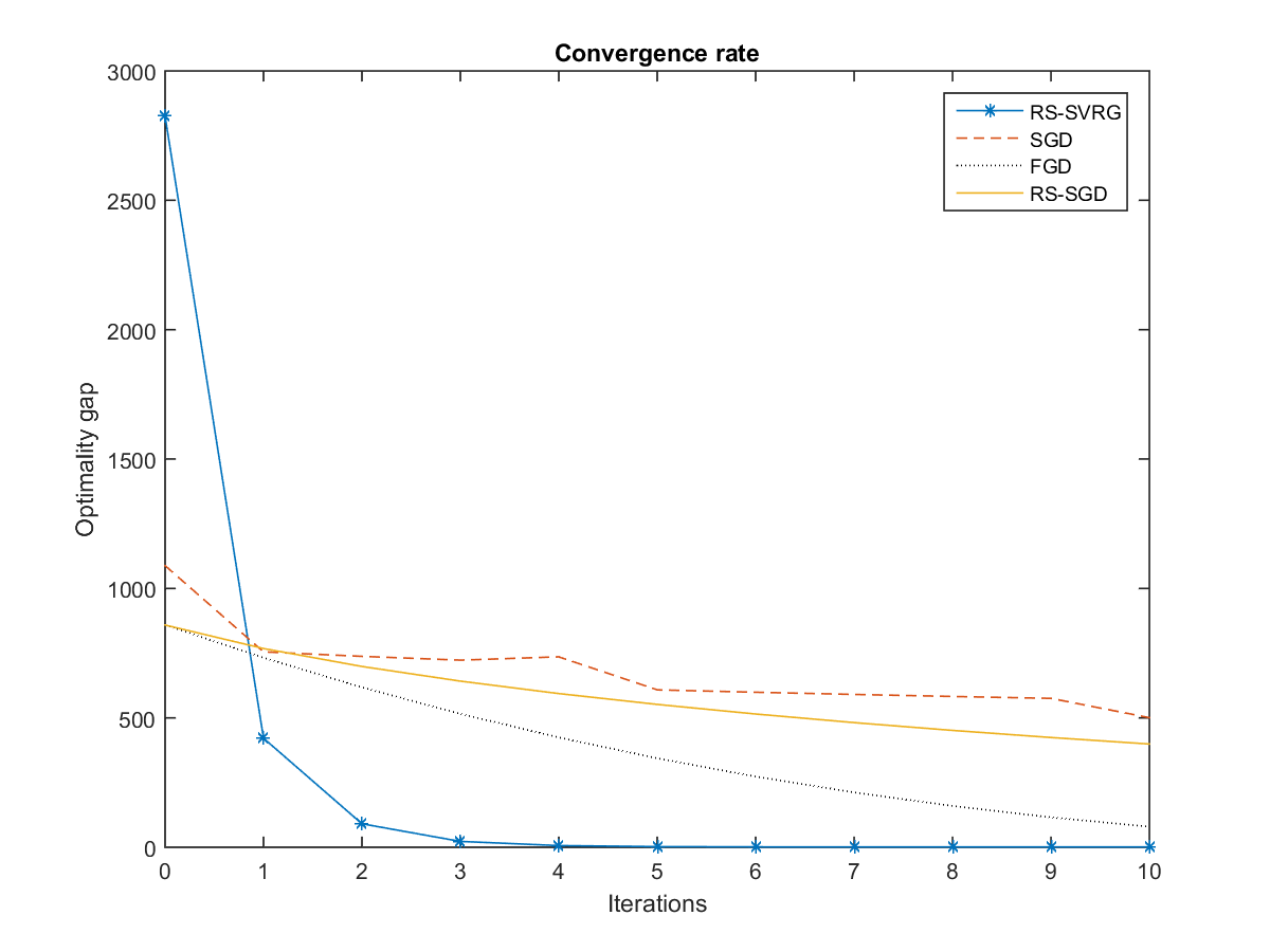
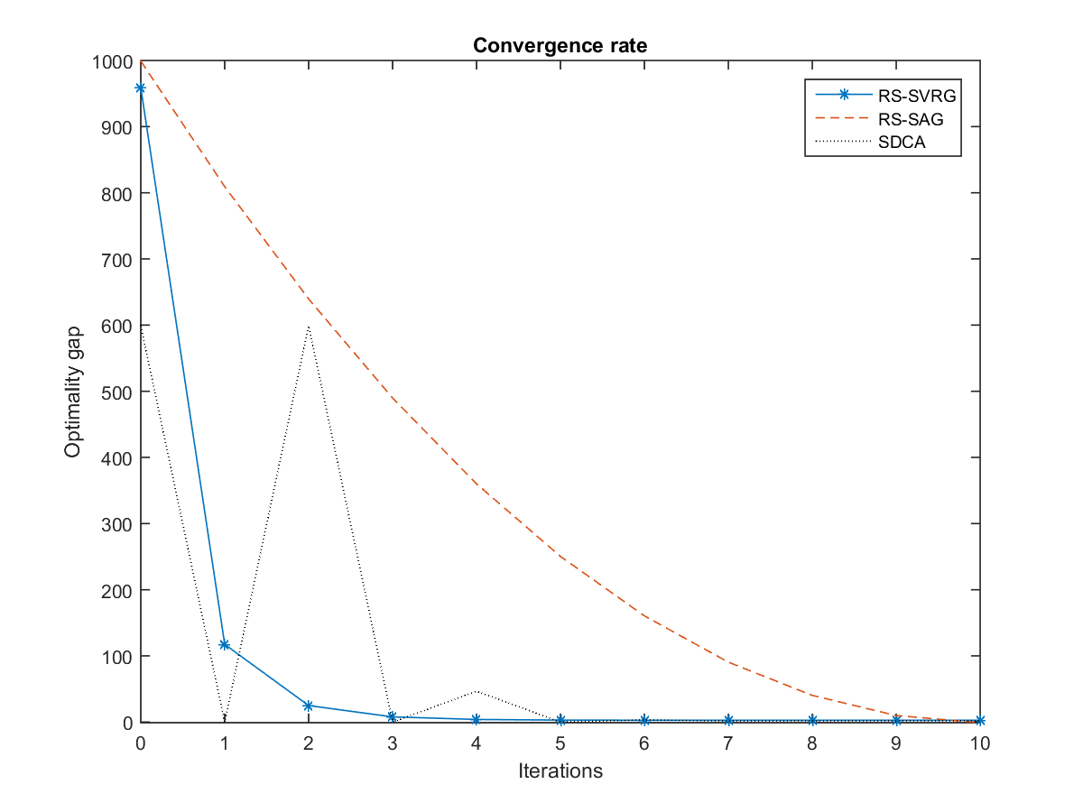
Figure 1: Ridge

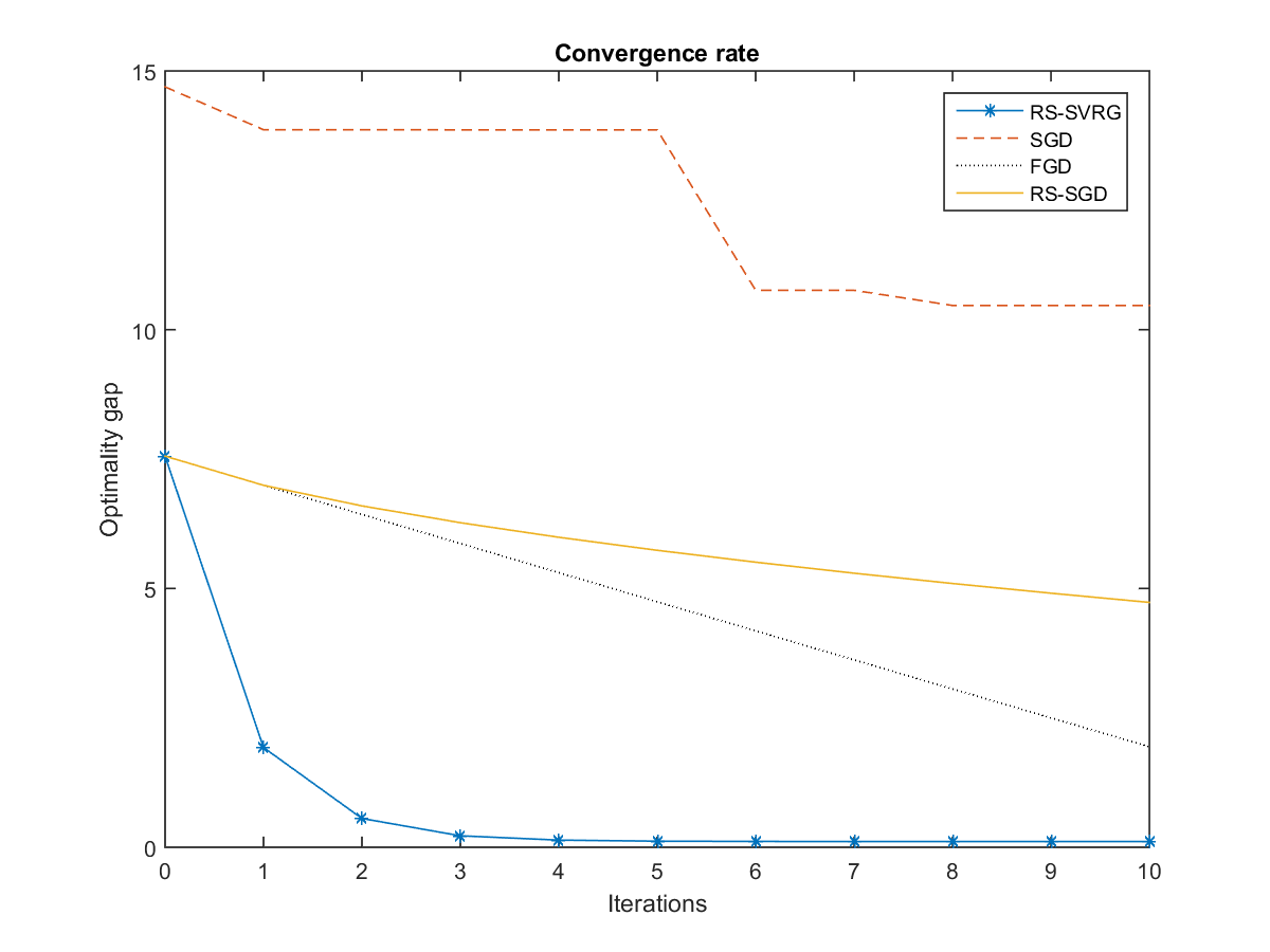
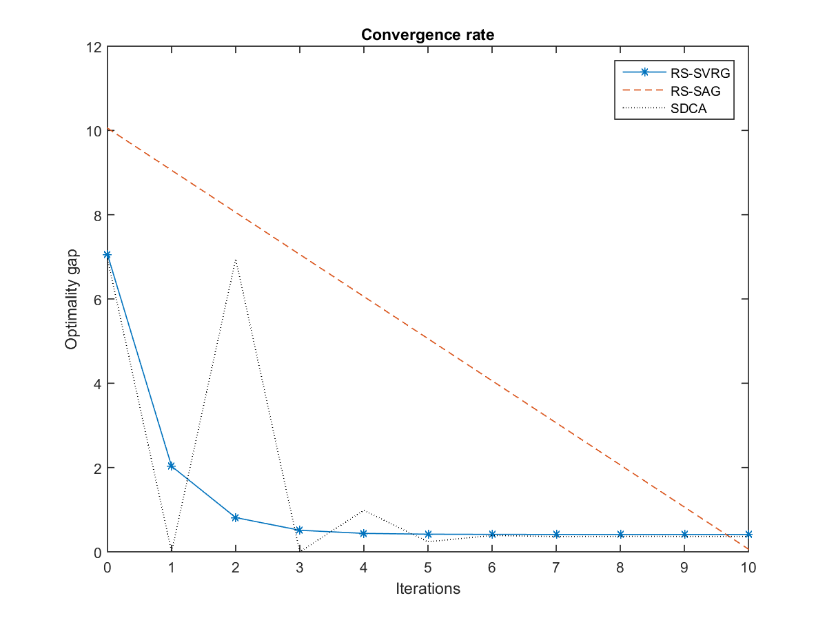
Figure 2: Lasso

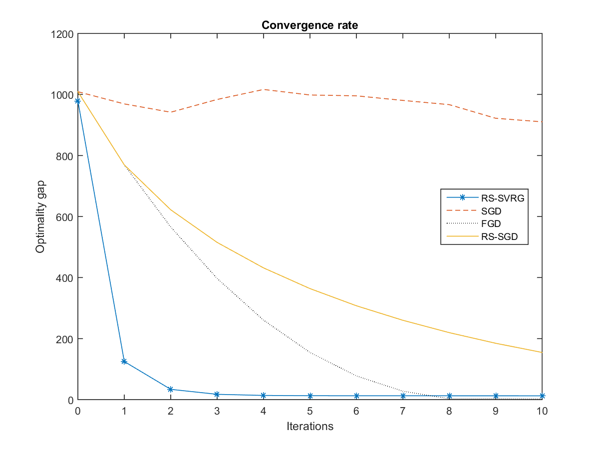
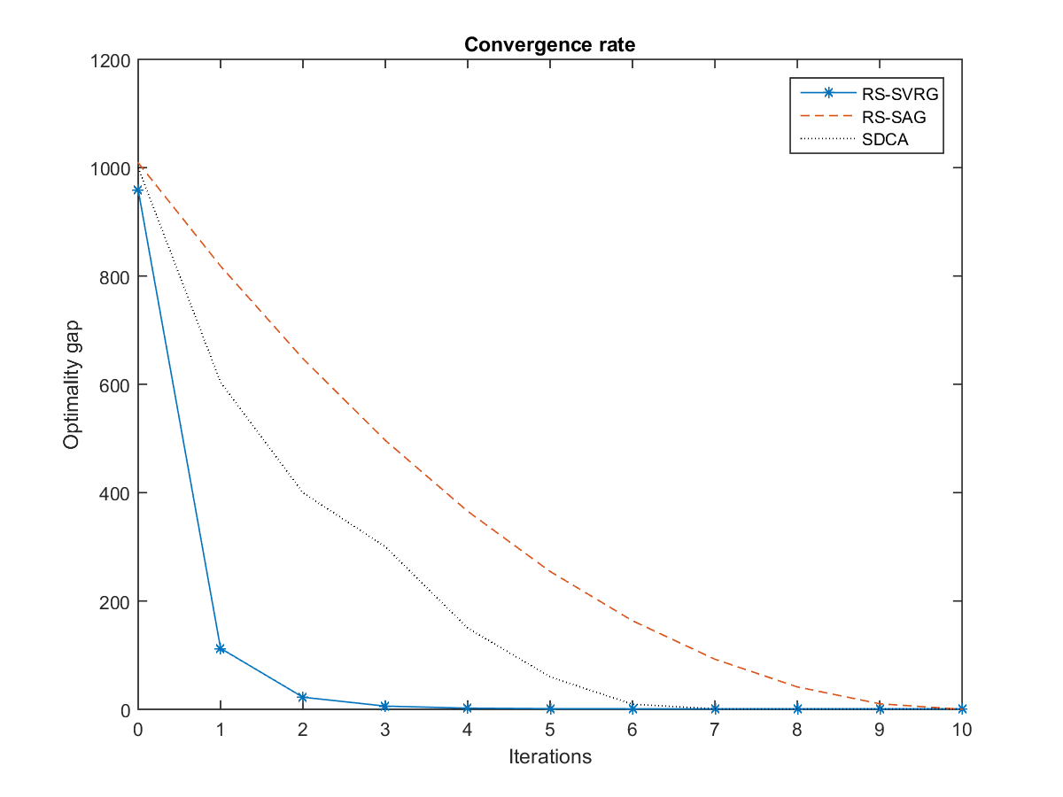
Figure 3: Elastic Net

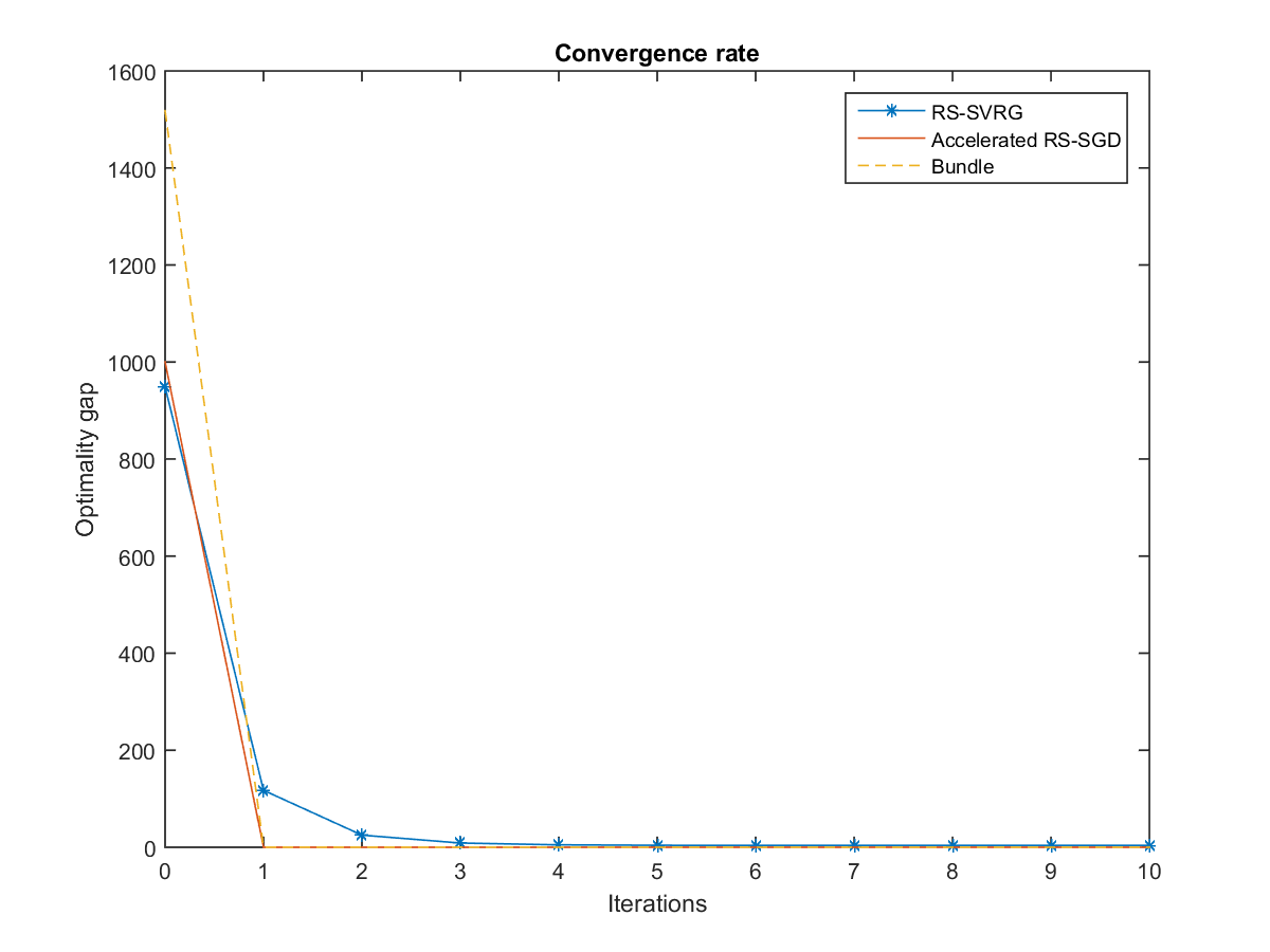
Figure 4: Comparison

$d$	$N$	$S$	RS-SVRG	A-RS-SGD	Bundle
$10$	$1000$	$10$	7.379s	1.102s	5.734s
$200$	$1000$	$10$	8.815s	1.217s	12.214s
$10$	$5000$	$100$	15.795s	23.242s	54.165s
$200$	$5000$	$100$	18.702s	23.022s	268.438s
$10$	$10000$	$10$	2.453s	2.767s	60.965s
$500$	$10000$	$10$	5.131s	5.349s	6562.426s

Table 1: Computational Time

3.2.2 Effects of sampling and problem dimension

In this section, we focus on ridge regularized problem, i.e., $\lambda_{1}=0.01,\,\lambda_{2}=0$ with different randomized sampling size $m$ and different problem dimension $d$. We study the effects of sampling and problem dimension under different choice of random sampling distribution $\mu$. Figure 5, show the results as predicted by our theory and discussion in Section 2, receiving more samples $m$ gives improvements in reducing the optimality gap as a function of iteration. The plots $m=50$ and $m=100$ are essentially indistinguishable, which implies that when the sampling size is large enough, there should be no obvious improvement in actual iteration taken to minimize the objective. Our theory also predicts that the upper bound for the convergence rate contains a term with $O(1/m$) from Corollaries 2.8, 2.9 and 2.10, which means that the improvement of optimality gap is deceasing as $1/m$ approaching zero. Figure 6 and 7 illustrate the performance of the algorithm with respect to the problem dimension $d$ when $\mu$ follows $N(0,\,I_{d\times d})$, and follows uniform distribution on $\mathcal{B}_{\infty}(0,\,1)$, respectively. The results reveal that the optimality gap increases significantly with the increase of problem dimension. Besides, Figure 6 shows the optimality gap grows approximately in linear relationship with $\sqrt{d}$, conforming to what we have stated in Corollaries 2.9. Figure 7 shows the optimality gap grows strictly linear with $d$, conforming to what we have stated in Corollaries 2.10.

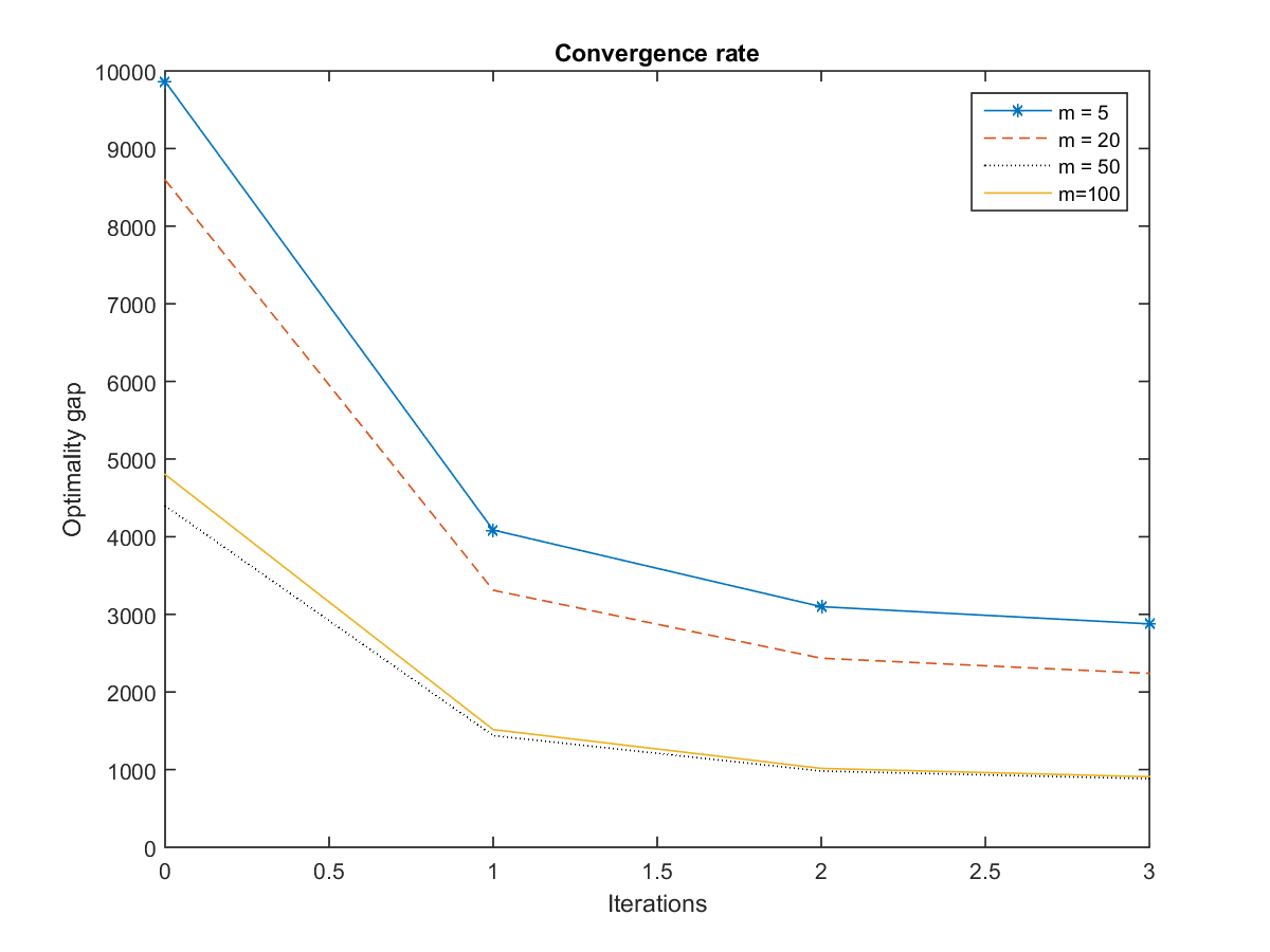
Figure 5: Effect of Samplings

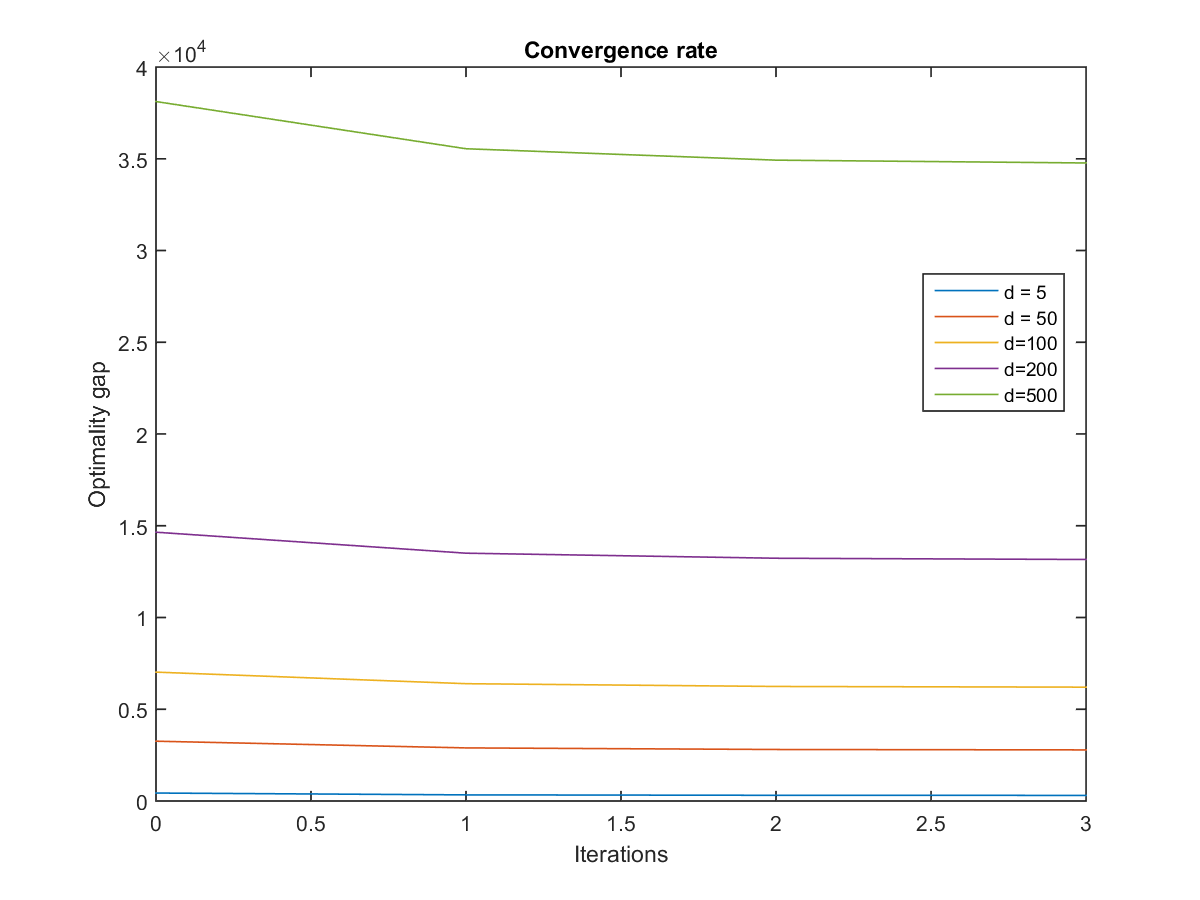
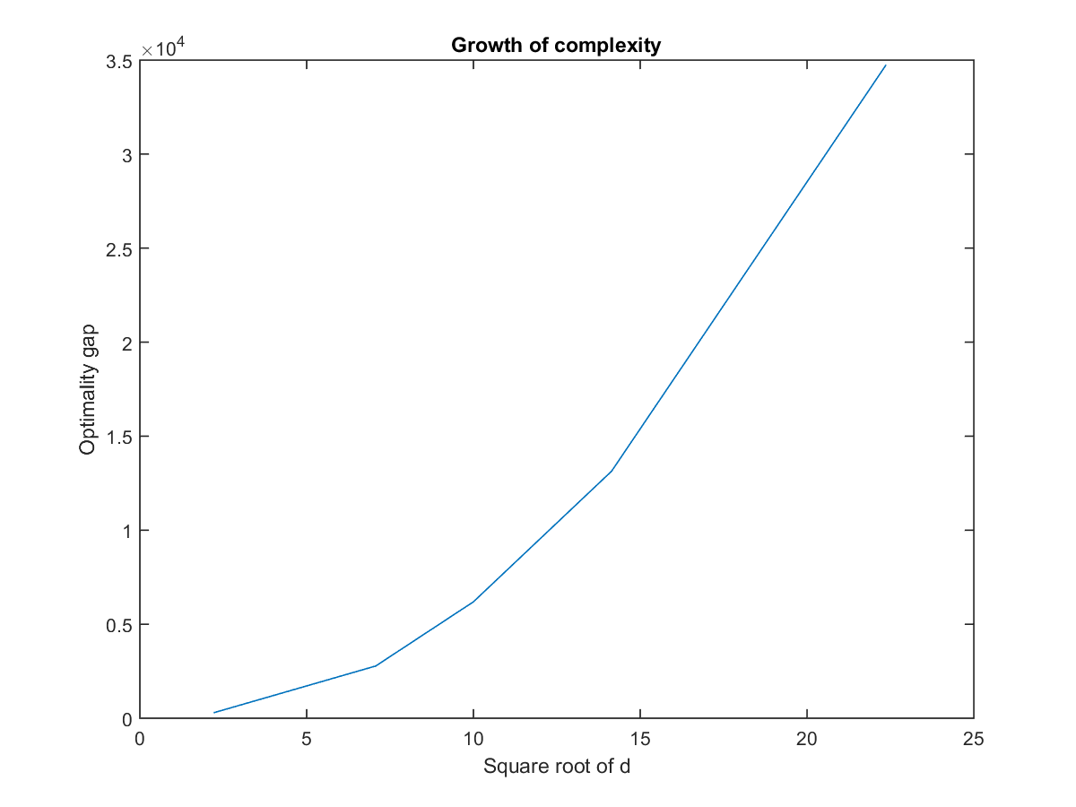
Figure 6: Effect of Dimension-$N(0,\,I_{d\times d})$

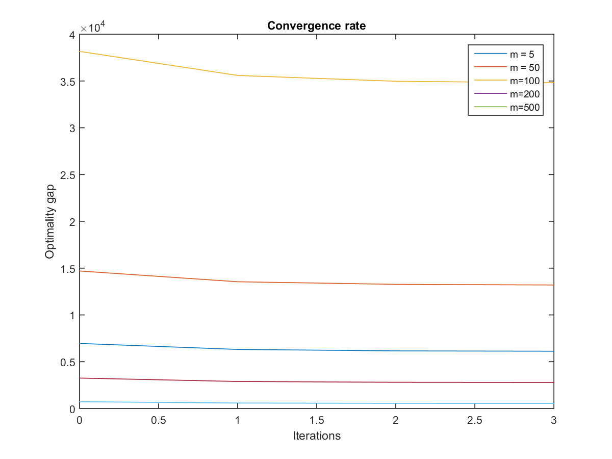
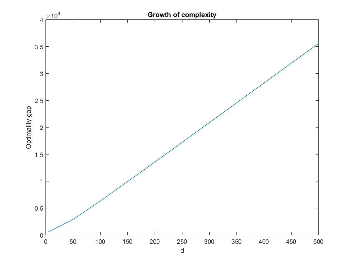
Figure 7: Effect of Dimension-Uniform on $B_{\infty}(0,\,1)$

4 Conclusion

In this paper, we develop and analyze a new method, for minimizing the sum of two convex functions: one is the average of a large number of convex component functions (not necessarily smooth and strongly-convex), and the other is a general convex function that admits a simple proximal mapping. Our RS-SVRG method uses randomized smoothing technique to smooth the component functions and exploits the finite average structure of the smooth part by extending the variance reduction technique of SVRG, which computes the full gradient periodically to modify the stochastic gradients in order to reduce their variance. We have given, to the best of our knowledge, the first variance reduction techniques for large-scale nonsmooth convex optimization.

From convergence analysis, we prove that RS-SVRG method enjoys linear convergence with constant convergence rate. Besides, it enjoys much lower time complexity and gradient complexity than gradient methods-stochastic subgradient descent and full subgradient descent. In addition, compared with some state-of-art nonsmooth algorithms including Nesterov’s smoothing and Bundle method, our method does not require the storage of the historical subgradient information on each component functions, which saves significant computational budge on large-scale and high dimensional problems. It should be noted that our method can be applied to a more general class of problems, without strongly-convex condition on objective and any other global and local error bound condition.

We study the effects of different smoothing distributions on our algorithm, and derive several corollaries outlining upper convergence rate bounds with the problem dimension and number of smoothing samples. Our experiments also show qualitatively good agreement with the theoretical predictions we have developed.

References

- Agarwal and Niyogi, 2009 Agarwal, S. and Niyogi, P. (2009). Generalization bounds for ranking algorithms via algorithmic stability. Journal of Machine Learning Research, 10(Feb):441–474.
- Allen-Zhu and Yuan, 2016 Allen-Zhu, Z. and Yuan, Y. (2016). Improved svrg for non-strongly-convex or sum-of-non-convex objectives. In International conference on machine learning, pages 1080–1089.
- Bach and Moulines, 2013 Bach, F. and Moulines, E. (2013). Non-strongly-convex smooth stochastic approximation with convergence rate o (1/n). In Advances in neural information processing systems, pages 773–781.
- Chen et al., 2012 Chen, H., He, F., and Pan, Z. (2012). Approximation analysis of gradient descent algorithm for bipartite ranking. Journal of Applied Mathematics, 2012.
- Duchi et al., 2012 Duchi, J. C., Bartlett, P. L., and Wainwright, M. J. (2012). Randomized smoothing for stochastic optimization. SIAM Journal on Optimization, 22(2):674–701.
- Gong and Ye, 2014 Gong, P. and Ye, J. (2014). Linear convergence of variance-reduced stochastic gradient without strong convexity. arXiv preprint arXiv:1406.1102.
- Herbrich et al., 2000 Herbrich, R., Graepel, T., and Obermayer, K. (2000). Large margin rank boundaries for ordinal regression. advances in large margin classifiers (pp. 115–132).
- Joachims, 2002 Joachims, T. (2002). Optimizing search engines using clickthrough data. In Proceedings of the eighth ACM SIGKDD international conference on Knowledge discovery and data mining, pages 133–142. ACM.
- Johnson and Zhang, 2013 Johnson, R. and Zhang, T. (2013). Accelerating stochastic gradient descent using predictive variance reduction. In Advances in neural information processing systems, pages 315–323.
- Johnstone and Moulin, 2017 Johnstone, P. R. and Moulin, P. (2017). Faster subgradient methods for functions with h" olderian growth. arXiv preprint arXiv:1704.00196.
- Kivinen et al., 2004 Kivinen, J., Smola, A. J., and Williamson, R. C. (2004). Online learning with kernels. IEEE transactions on signal processing, 52(8):2165–2176.
- Le et al., 2008 Le, Q. V., Smola, A. J., and Vishwanathan, S. (2008). Bundle methods for machine learning. In Advances in neural information processing systems, pages 1377–1384.
- Lucchi et al., 2015 Lucchi, A., McWilliams, B., and Hofmann, T. (2015). A variance reduced stochastic newton method. arXiv preprint arXiv:1503.08316.
- Mairal, Mairal, J. A generic quasi-newton algorithm for faster gradient-based optimization.
- Mäkelä, 2002 Mäkelä, M. (2002). Survey of bundle methods for nonsmooth optimization. Optimization methods and software, 17(1):1–29.
- Mifflin et al., 1998 Mifflin, R., Sun, D., and Qi, L. (1998). Quasi-newton bundle-type methods for nondifferentiable convex optimization. SIAM Journal on Optimization, 8(2):583–603.
- Moritz et al., 2016 Moritz, P., Nishihara, R., and Jordan, M. (2016). A linearly-convergent stochastic l-bfgs algorithm. In Artificial Intelligence and Statistics, pages 249–258.
- Nedić and Bertsekas, 2001 Nedić, A. and Bertsekas, D. (2001). Convergence rate of incremental subgradient algorithms. In Stochastic optimization: algorithms and applications, pages 223–264. Springer.
- Nesterov, 2005 Nesterov, Y. (2005). Smooth minimization of non-smooth functions. Mathematical programming, 103(1):127–152.
- Robinson, 1999 Robinson, S. M. (1999). Linear convergence of epsilon-subgradient descent methods for a class of convex functions. Mathematical Programming, 86(1):41–50.
- Schmidt et al., 2017 Schmidt, M., Le Roux, N., and Bach, F. (2017). Minimizing finite sums with the stochastic average gradient. Mathematical Programming, 162(1-2):83–112.
- Shai-Shwartz et al., 2004 Shai-Shwartz, S., Singer, Y., and Ng, A. (2004). Online and batch learning of pseudo-metrics. In Machine Learning, Proceedings of the Twenty-first International Conference (ICML 2004). ACM Press, New York, NY.
- Shalev-Shwartz et al., 2009 Shalev-Shwartz, S., Shamir, O., Srebro, N., and Sridharan, K. (2009). Stochastic convex optimization. In COLT.
- Shalev-Shwartz and Zhang, 2012 Shalev-Shwartz, S. and Zhang, T. (2012). Proximal stochastic dual coordinate ascent. arXiv preprint arXiv:1211.2717.
- Shalev-Shwartz and Zhang, 2013 Shalev-Shwartz, S. and Zhang, T. (2013). Stochastic dual coordinate ascent methods for regularized loss minimization. Journal of Machine Learning Research, 14(Feb):567–599.
- Shamir and Zhang, 2013 Shamir, O. and Zhang, T. (2013). Stochastic gradient descent for non-smooth optimization: Convergence results and optimal averaging schemes. In International Conference on Machine Learning, pages 71–79.
- Shen et al., 2013 Shen, J., Pang, L.-P., and Li, D. (2013). An approximate quasi-newton bundle-type method for nonsmooth optimization. In Abstract and Applied Analysis, volume 2013. Hindawi.
- Vainsencher et al., 2015 Vainsencher, D., Liu, H., and Zhang, T. (2015). Local smoothness in variance reduced optimization. In Advances in Neural Information Processing Systems, pages 2179–2187.
- Xiao, 2010 Xiao, L. (2010). Dual averaging methods for regularized stochastic learning and online optimization. Journal of Machine Learning Research, 11(Oct):2543–2596.
- Xiao and Zhang, 2014 Xiao, L. and Zhang, T. (2014). A proximal stochastic gradient method with progressive variance reduction. SIAM Journal on Optimization, 24(4):2057–2075.
- Xing et al., 2003 Xing, E. P., Jordan, M. I., Russell, S. J., and Ng, A. Y. (2003). Distance metric learning with application to clustering with side-information. In Advances in neural information processing systems, pages 521–528.
- Xu et al., 2017 Xu, Y., Lin, Q., and Yang, T. (2017). Stochastic convex optimization: Faster local growth implies faster global convergence. In International Conference on Machine Learning, pages 3821–3830.
- Yang and Lin, 2015a Yang, T. and Lin, Q. (2015a). Rsg: Beating subgradient method without smoothness and strong convexity. arXiv preprint arXiv:1512.03107.
- Yang and Lin, 2015b Yang, T. and Lin, Q. (2015b). Stochastic subgradient methods with linear convergence for polyhedral convex optimization. arXiv preprint arXiv:1510.01444.