Initial Access Frameworks for
3GPP NR at mmWave Frequencies

Abstract

The use of millimeter wave (mmWave) frequencies for communication will be one of the innovations of the next generation of cellular mobile networks (5G). It will provide unprecedented data rates, but is highly susceptible to rapid channel variations and suffers from severe isotropic pathloss. Highly directional antennas at the transmitter and the receiver will be used to compensate for these shortcomings and achieve sufficient link budget in wide area networks. However, directionality demands precise alignment of the transmitter and the receiver beams, an operation which has important implications for control plane procedures, such as initial access, and may increase the delay of the data transmission. This paper provides a comparison of measurement frameworks for initial access in mmWave cellular networks in terms of detection accuracy, reactiveness and overhead, using parameters recently standardized by the 3GPP and a channel model based on real-world measurements. We show that the best strategy depends on the specific environment in which the nodes are deployed, and provide guidelines to characterize the optimal choice as a function of the system parameters.

I Introduction

The 5th generation (5G) of mobile cellular networks is currently being standardized by the 3GPP as NR [1], and is designed to enable a fully mobile and connected society, in order to address the tremendous growth in connectivity and density/volume of traffic that will be required in the near future [2]. In particular, 5G cellular networks are designed to provide very high throughput (1 Gbps or more), ultra-low latency (even less than 1 ms in some cases), ultra-high reliability, low energy consumption, and ultra-high connectivity resilience [2].

The mmWave spectrum – roughly comprised between 10 and 300 GHz – has been considered as an enabler of the 5G performance requirements in micro and picocellular networks [3]. These frequencies offer much more bandwidth than current cellular systems, which are allocated in the congested bands below 6 GHz, and initial capacity estimates have suggested that mmWave networks offer orders of magnitude higher bit-rates than 4G systems [4]. However, the increased carrier frequency makes the propagation conditions more demanding than at the lower frequencies traditionally used for wireless services, making the communication less reliable [5]. MmWave signals suffer from a higher pathloss and severe channel intermittency, and are blocked by many common materials [6]. As a result, the quality of the wireless link between the User Equipment (UE) and the network can be highly variable.

To overcome these limitations, next-generation cellular systems will be equipped with high-dimensional phased arrays both at the UE and at the Next Generation Node Base Station (gNB), in order to establish highly directional transmission links and to benefit from the resulting beamforming gain. Directional links, however, require fine alignment of the transmitter and the receiver beams, a procedure which might greatly increase the time it takes to access the network. In this regard, defining efficient Initial Access (IA) procedures, which allow a mobile UE to establish a physical link connection with a gNB (a necessary step to access the network), is particularly challenging at mmWave frequencies [7]. In current Long Term Evolution (LTE) systems, IA is performed on omnidirectional channels, whereas beamforming or other directional transmissions can only be performed after a physical link is established [8]. On the other hand, in the mmWave bands, it may be essential to exploit the antenna gains already during the IA phase, otherwise there would be a mismatch between the range at which a cell can be detected (control-plane range), and the much longer range at which a user could directionally send and receive data using beamforming (user-plane range).

I-A Related Work

Papers on IA (e.g., [7, 9]) in 5G mmWave cellular systems are very recent. Most literature refers to lower frequencies in ad hoc wireless network scenarios or, more recently, to the 60 GHz IEEE 802.11ad WLAN and WPAN scenarios (e.g., [11]). However, most of the proposed solutions present many limitations (e.g., they are appropriate for short-range, static and indoor scenarios) which prevent them from matching the requirements of cellular systems.

Recently, new solutions specifically designed for mobile wireless networks have been proposed. In [12, 13], the authors proposed an exhaustive method that performs IA over mmWave frequencies by periodically transmitting directional synchronization signals to scan the angular space. With this approach, a large number of antennas at the transceiver makes it possible to reach more users with respect to the case with a single omnidirectional antenna, at the cost of a longer delay for the IA. Additionally, more sophisticated discovery techniques (e.g., [14]) decrease the exhaustive search delay through a multi-phase hierarchical procedure, in which access signals are first sent over a few directions, with wide beams, and then iteratively refined until the beamforming gain is sufficiently high. In [15] a low-complexity beam selection method is derived by exploiting the sparsity of mmWave channels, and thanks to compressive sensing it is possible to avoid explicit channel estimation for beam management.

The performance of the association techniques also depends on the beamforming architecture implemented in the transceivers. Preliminary works aiming at finding the optimal beamforming strategy refer to WLAN scenarios. For example, the algorithm proposed in [16] takes into account the spatial distribution of nodes, to allocate the beamwidth of each antenna pattern in an adaptive fashion and satisfy the required link budget criterion. Since the proposed algorithm minimizes the collisions, it also minimizes the average time required to transmit a data packet from the source to the destination through a specific direction. In 5G scenarios, papers [12, 13, 14] give some insights on tradeoffs among different beamforming architectures in terms of user association’s quality.

I-B Contributions of This Paper

In this paper we provide the first global comprehensive evaluation of mmWave measurement frameworks for IA, using 3GPP NR scenario configurations (e.g., the NR frame structure and other relevant physical-layer parameters), and assess how to optimally design fast, accurate and robust control-plane management schemes through measurement reports. We focus on Downlink (DL) and Uplink (UL) frameworks, and on Standalone (SA) and Multi-Connectivity (MC) architectures. We simulate their performance in terms of (i) detection accuracy, i.e., how representative the measurement is; (ii) reactiveness, i.e., how quickly a mobile user gets access to the network; and (iii) overhead, i.e., how many resources are needed for the measurement operations. Finally, we illustrate some of the complex tradeoffs to be considered when designing IA solutions for 3GPP NR. The results prove that the optimal design for implementing efficient and fast IA must account for several specific features such as the gNBs density, the antenna geometry, the beamforming configuration and the level of integration and harmonization of different technologies.

The rest of the paper is organized as follows. In Sec. II we provide an introduction on 3GPP NR procedures for IA at mmWave frequencies, and present the IA frameworks we will evaluate. In Sec. III we describe the system model, the metrics that will be considered and the 3GPP parameters that will be configured. In Sec. IV we present our main findings and results, while Sec. V concludes the paper.

II Initial Access Frameworks

3GPP NR will support a wide range of frequencies and use cases, and is designed to support beamforming operations for both data and control planes [1] in the Physical (PHY) and Medium Access Control (MAC) layers. In particular, for IA, the concept of Synchronization Signal (SS) block and burst recently emerged for the periodic transmission of synchronization signals from the gNBs [17]. These signals can be used at the receiver side to estimate the channel and select the best gNB to attach to. An SS block is a group of 4 Orthogonal Frequency Division Multiplexing (OFDM) symbols in time and 240 subcarriers in frequency [17], and carries the Primary Synchronization Signal (PSS), the Secondary Synchronization Signal (SSS) and the Physical Broadcast Channel (PBCH). The DeModulation Reference Signal (DMRS) associated with the PBCH can be used to estimate the Reference Signal Received Power (RSRP) of each SS block. For each slot of 14 symbols there can be up to two SS blocks [17]. The SS blocks are grouped in an SS burst, which lasts up to 5 ms, and can be repeated after $T_{\rm SS}\in\{5,10,20,40,80,160\}$ ms [18]. The maximum number $L$ of SS blocks in a burst is frequency-dependent [17], and above 6 GHz there could be up to 64 blocks per burst. When considering frequencies for which beam operations are required, each SS block is mapped to a certain angular direction.

Moreover, 3GPP NR specifications include a set of basic procedures for beam management [1]. We analyze two different deployment architectures. With the standalone option, the UE connects only to an NR gNB at mmWave frequencies. With multi-connectivity, instead, each UE maintains multiple possible signal paths to different cells at different frequencies (e.g., NR at mmWave and LTE at conventional frequencies), thus providing both high capacity and robust connections [19]. We also distinguish between a downlink and an uplink framework. In the downlink case, the gNBs transmit synchronization signals (i.e., SS blocks) which are collected by the surrounding UEs, while in the uplink case the measurements are based on Sounding Reference Signals (SRSs) transmitted by the mobile terminals. Notice that the 3GPP considers only the downlink framework for IA. Nonetheless, it is worth comparing the downlink and uplink solutions, given that the rising heterogeneity in cellular networks is dramatically changing the traditional notion of a communication cell [2], increasing the importance of the uplink traffic and advocating the design of UL-driven solutions for both the data and the control planes.

The first procedure for IA is beam sweeping, i.e., covering a spatial area with a set of beams transmitted and received according to pre-specified intervals and directions. The second procedure, denominated beam measurement, requires the UEs in a downlink framework (or the gNBs in an uplink one) to evaluate the quality of the received signal. Different metrics could be used [20]. In this paper, we consider the Signal to Noise Ratio (SNR), which is the linear average of the received power on different resources with synchronization signals divided by the noise power. The third procedure is beam determination, i.e., the selection of the best beams at the gNB and at the UE, according to the measurements obtained with the beam measurement procedure. This procedure differs in the DL and UL frameworks. In downlink, the UE performs autonomously a decision on the best direction in which IA should be performed. In uplink, instead, the gNBs forward the channel measurements to a central controller, which then decides which is the best direction. The fourth and final procedure is beam reporting, i.e., information on the quality of the received beamformed signals and on the decisions in the beam determination phase is exchanged. In a standalone downlink (SA-DL) framework, as proposed by the 3GPP, the mobile terminal has to wait for the gNB to schedule the Random Access Channel (RACH) opportunity towards the best direction that the UE has just determined, for performing random access and implicitly informing the selected serving infrastructure about the optimal direction through which it has to steer its beam. As reported in [21], it has been agreed that for each SS block the gNB will specify one or more RACH opportunities with a certain time and frequency offset and direction, so that the UE knows when to transmit the RACH preamble. When a multi-connectivity downlink (MC-DL) scheme is considered, instead, the UE can use the LTE connection to report the optimal set of directions to the gNBs, so that it does not need to wait for an additional beam sweep from the gNB to perform the beam reporting or the IA procedure. Similarly, in a multi-connectivity uplink (MC-UL) framework, the network reports to the UE the optimal direction and the resources for random access. Notice that we do not consider the SA-UL configuration for IA, since we believe that uplink-based architectures will likely necessitate the support of an LTE overlay for the management of the control plane and the implementation of efficient measurement operations.

III System Model

III-A Performance Metrics

The performance of the different architectures and beam management procedures for IA will be assessed using three different metrics. The detection accuracy is measured in terms of probability of misdetection $P_{\rm MD}$, defined as the probability that the UE is not detected by the base station (i.e., the maximum SNR is below a threshold $\Gamma$) in an uplink scenario, or, vice versa, the base station is not detected by the UE in a downlink scenario after a complete beam sweeping in all the available directions. The reactiveness is the average time to find and report the best beam pair for IA, i.e., the time needed to perform the beam management procedures for IA described in the previous section. Finally, the overhead is the amount of time and frequency resources allocated to the framework with respect to the total amount of available resources.

The simulations for the detection accuracy performance evaluation are based on realistic system design configurations where multiple gNBs are deployed according to a Poisson Point Process. The channel model is based on recent real-world measurements at 28 GHz in New York City, to provide a realistic assessment of mmWave micro and picocellular networks in a dense urban deployment [22].

III-B 3GPP Framework Parameters

In this section, we list the parameters that affect the performance of the measurement architectures, and provide insights on the impact of each parameter on the different metrics.

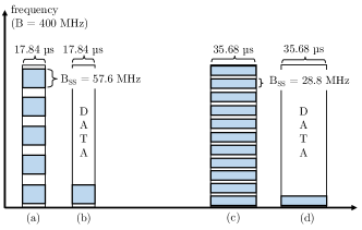
Fig. 1: SS block structure. Each blue rectangle is an SS block (with 4 OFDM symbols). Cases (a) and (c) implement a frequency repetition scheme (with $N_{rep}=5$ and $11$, respectively) while, for cases (b) and (d), a data solution (i.e., $N_{rep}=1$) is preferred.

As depicted in Fig. 1, we consider the frame structure of 3GPP NR, with different subcarrier spacings $\Delta_{f}$. For frequencies above 6 GHz, the subcarrier spacing $\Delta_{f}$ is $15\times 2^{n}$ kHz, with $2\leq n\leq 4$ (i.e., $\Delta_{f}=60$, 120 or 240 kHz) and 14 OFDM symbols per slot. The slot duration in $\mu$s is given by $T_{\rm slot}=1000/2^{n}$, while the duration of a symbol in $\mu$s is $T_{\rm symb}=71.42/2^{n}$ [17]. Since the only subcarrier spacings considered for frequencies above 6 GHz are $\Delta_{f}=120$ and $240$ kHz, we will only consider these cases. Therefore, the slot duration is $125~{}\mu$s or $62.5~{}\mu$s, respectively. Moreover, since the maximum number of subcarriers allocated to the SS blocks is 240, then the bandwidth allocated for the SS blocks would be respectively 28.8 and 57.6 MHz. We consider a maximum channel bandwidth $B=400$ MHz per carrier.

Moreover, it is possible to configure the system to exploit frequency diversity, $D$. Given that 240 subcarriers are allocated in frequency to an SS, the remaining bandwidth in the symbols which contain an SS block is $B-240\Delta_{f}$. Therefore, it is possible to adopt two different strategies: (i) data (as represented in Figs. 1(b) and (d)), i.e., it is used for data transmission towards users which are in the same direction in which the SS block is transmitted, or (ii) repetition (as displayed in Figs. 1(a) and (c)), i.e., the information in the first 240 subcarriers is repeated in the remaining subcarriers to increase the robustness against noise and enhance the detection capabilities. The number of repetitions is therefore $N_{rep}=1$ if frequency diversity is not used (i.e., $D=0$, and a single chunk of the available bandwidth is used for the SS block), and $N_{rep}=11$ or $N_{rep}=5$ when repetition is used (i.e., $D=1$) with $\Delta_{f}=120$ kHz or $\Delta_{f}=240$ kHz, respectively. There is a guard interval in frequency among the different repetitions of the SS blocks, to provide a good tradeoff between frequency diversity and coherent combining [13].

We also consider different configurations of the SS blocks and bursts. The maximum number $N_{\rm SS}$ of SS blocks in a burst for our frame structure and carrier frequencies is $L=64$. We assume that, if $N_{\rm SS}<L$, the SS blocks will be transmitted in the first $N_{\rm SS}$ opportunities. The actual maximum duration of an SS burst is $D_{\max,\rm SS}=2.5$ ms for $\Delta_{f}=240$ kHz and $D_{\max,\rm SS}=5$ ms for $\Delta_{f}=120$ kHz. We will also investigate all the possible values for the SS burst periodicity $T_{\rm SS}$.

Another fundamental parameter is the array geometry, i.e., the number of antenna elements $M$ at the gNB and UE and the number of directions that need to be covered, both in azimuth $N_{\theta}$ and in elevation $N_{\phi}$. At the gNB we consider a single sector in a three-sector site, i.e., the azimuth $\theta$ varies from $-60$ to $60$ degrees, for a total of $\Delta_{\theta}=120$ degrees, while the UE has a single array panel which covers the whole $\Delta_{\theta,\rm UE}=360^{\circ}$ angular space. The elevation $\phi$ varies between $-30$ and $30$ degrees, for a total of $\Delta_{\phi}=60$ degrees, and also includes a fixed mechanical tilt of the array pointing towards the ground. There exists a strong correlation among beamwidth, number of antenna elements and beamforming gain. The more antenna elements in the system, the narrower the beams, the higher the gain that can be achieved by beamforming, and the more precise and directional the transmission. Thus, given the array geometry, we compute the beamwidth $\Delta_{\rm beam}$ at 3 dB of the main lobe of the beamforming vector, and then $N_{\theta}=\Delta_{\theta}/\Delta_{\rm beam}$ and $N_{\phi}=\Delta_{\phi}/\Delta_{\rm beam}$. The results are shown in Table I.

$M$	$\theta$ [deg]	$N_{\theta}$ gNB	$N_{\theta}$ UE
4	60	2	6
16	26	5	14
64	13	10	28

TABLE I: Relationship between $M$, $\theta$ and $N_{\theta}$, for the azimuth case [10].

Additionally, different beamforming architectures, i.e., analog, hybrid or digital, can be used both at the UE and at the gNB. Analog beamforming shapes the beam through a single Radio Frequency (RF) chain for all the antenna elements and therefore it is possible to transmit/receive in only one direction at any given time. This model saves power by using only a single pair of Analog to Digital Converters (ADCs), but has small flexibility since the transceiver can only beamform in one direction. Hybrid beamforming uses $K_{\rm BF}$ RF chains (with $1<K_{\rm BF}\leq M$), and thus is equivalent to $K_{\rm BF}$ parallel analog beams, as it enables the transceiver to transmit/receive in $K_{\rm BF}$ directions simultaneously. Nevertheless, when hybrid beamforming is used for transmission, the power available at each transmitting beam is the total node power constraint divided by $K_{\rm BF}$, thus potentially reducing the received power. Digital beamforming requires a separate RF chain for each antenna element and therefore allows the processing of the received signals in the digital domain, potentially enabling the transceiver to direct beams at infinitely many directions at the same time [23]. Although the digital transceiver is able to process an infinite number of received streams, only $M$ simultaneous and orthogonal beams can be handled without significant inter-beam interference (i.e., through a zero-forcing beamforming structure [24]). For this reason, we limit the number of parallel beams that can be generated to $M$. Furthermore, for energy-saving purposes, we implement a digital beamforming scheme only at the receiver side. For the sake of completeness, we also consider an omnidirectional strategy at the UE, i.e., without any beamforming gain but allowing the reception through the whole angular space at any given time.

Finally, the last parameter is the density of base stations $\lambda_{b}$, expressed in gNB/km².

IV Results and Discussion

In this section, we present some simulation results aiming at (i) evaluating the performance of the presented IA schemes in terms of detection accuracy (i.e., probability of misdetection), as reported in Sec. IV-A; (ii) describing the analysis and the results related to the performance of the measurement frameworks for the reactiveness and the overhead, respectively in Sec. IV-B and Sec. IV-C. Final considerations and remarks, aimed at providing guidelines to characterize the optimal IA configuration settings as a function of the system parameters, are contained in Sec. IV-D.

IV-A Detection Accuracy Results

In Fig. 2 we plot the Cumulative Distribution Function (CDF) of the SNR between the mobile terminal and the gNB it is associated to, for different antenna configurations and considering two density values. Notice that the curves are not smooth because of the progressive transitions of the SNR among the different path loss regimes, i.e., Line of Sight (LOS), Non Line of Sight (NLOS) and outage. We see that better detection accuracy performance can be achieved when densifying the network and when using larger arrays. In the first case, the endpoints are progressively closer, thus ensuring better signal quality and, in general, stronger received power. In the second case, narrower beams can be steered thus guaranteeing higher beamforming gains. We also notice that, for good SNR regimes, the $M_{\rm gNB}=4,M_{\rm UE}=4$ and $M_{\rm gNB}=64,M_{\rm UE}=4$ configurations present good enough SNR values: in these regions, the channel conditions are sufficiently good to ensure satisfactory signal quality (and, consequently, acceptable misdetection) even when considering small antenna factors. Finally, the red line represents the SNR threshold $\Gamma=-5$ dB that we will consider in this work.

Fig. 2: CDF of the SNR, for different antenna configurations. $\Delta_{f}=120$ kHz, $N_{rep}=1$. The red dashed line represents the SNR threshold $\Gamma=-5$ dB that has been considered throughout this work.

Fig. 3: $P_{\rm MD}$ as a function of $\lambda_{b}$, for different antenna configurations.

Fig. 4: $P_{\rm MD}$ as a function of $\lambda_{b}$, for different subcarrier spacings $\Delta_{f}$ and repetition strategies and for different antenna configurations. $M_{\rm gNB}=4,M_{\rm UE}=4$, $\Gamma=-5$ dB.

Analogous considerations can be deduced from Fig. 3 which illustrates how the misdetection probability monotonically decreases when the gNB density $\lambda_{b}$ progressively increases or when the transceiver is equipped with a larger number of antenna elements, since more focused beams can be generated in this case. Moreover, we notice that the beamforming strategy in which the UE transmits or receives omnidirectionally, although guaranteeing fast access operations, does not ensure accurate IA performance and leads to degraded detection capabilities. More specifically, the gap with a fully directional architecture (e.g., $M_{\rm gNB}=64,M_{\rm UE}=16$) is quite remarkable for very dense scenarios, and increases as the gNB density increases. For example, the configuration with 16 antennas (i.e., $M_{\rm UE}=16$) and that with a single omnidirectional antenna at the UE reach the same $P_{\rm MD}$, but at different values of gNB density $\lambda_{b}$, respectively 30 and 35 $[\text{gNB/km}^{\text{2}}]$: the omnidirectional configuration requires a higher density (i.e., 5 $[\text{gNB/km}^{\text{2}}]$ more) to compensate for the smaller beamforming gain.

Finally, Fig. 4 reports the misdetection probability related to $\lambda_{b}$, for different subcarrier spacings $\Delta_{f}$ and repetition strategies $D$. First, we see that, if no repetitions are used (i.e., $D=0$), lower detection accuracy performance is associated with the $\Delta_{f}=240$ kHz configuration, due to the resulting larger impact of the thermal noise and the consequent SNR degradation. Furthermore, the detection efficiency can be enhanced by repeating the SS block information embedded in the first 240 subcarriers in the remaining subcarriers (i.e., $D=1$), to increase the robustness of the communication and mitigate the effect of the noise in the detection process. In fact, if a frequency diversity approach is preferred, the UE (in the DL measurement technique) or the gNB (in the UL measurement technique) has $N_{rep}>1$ attempts to properly collect the synchronization signals exchanged during the beam sweeping phase, compared to the single opportunity the nodes would have had if they had not implemented any repetition strategy. We also observe that the $\Delta_{f}=120$ kHz with no frequency diversity configuration and the $\Delta_{f}=240$ kHz scheme with $N_{rep}=5$ produce the same detection accuracy results, thus showing that increasing the subcarrier spacing and increasing the number of repetitions of the SS block information in multiple frequency subbands have almost the same effect in terms of misdetection capabilities. Finally, we observe that the impact of the frequency diversity $D$ and the subcarrier spacing $\Delta_{f}$ is less significant when increasing the array factor, as can be seen from the reduced gap between the curves plotted in Fig. 4 for the $M_{\rm gNB}=4,M_{\rm UE}=4$ and $M_{\rm gNB}=64,M_{\rm UE}=4$ configurations. The reason is that, when considering larger arrays, even the configuration with $\Delta_{f}=240$ kHz, with no repetitions, has an average SNR which is high enough to reach small misdetection probability values.

IV-B Reactiveness Results

For IA, reactiveness is defined as the delay required to perform a full iterative search in all the possible combinations of the directions. The gNB and the UE need to scan respectively $N_{\theta,\rm gNB}N_{\phi,\rm gNB}$ and $N_{\theta,\rm UE}N_{\phi,\rm UE}$ directions to cover the whole horizontal and vertical space. Moreover, they can transmit or receive respectively $K_{\rm BF,gNB}$ and $K_{\rm BF,UE}$ beams simultaneously. Notice that, as mentioned in Sec. III, for digital and omnidirectional architectures $K_{\rm BF}=\min\{N_{\theta}N_{\phi},M\}$, for hybrid $K_{\rm BF}=\min\{N_{\theta}N_{\phi},M\}/\nu$, where $\nu$ is a factor that limits the number of directions in which it is possible to transmit or receive at the same time, and for analog $K_{\rm BF}=1$ [25]. Then the total number of SS blocks needed is

$$S_{D}=\left\lceil\frac{N_{\theta,\rm gNB}N_{\phi,\rm gNB}}{K_{\rm BF,gNB}}\right\rceil\left\lceil\frac{N_{\theta,\rm UE}N_{\phi,\rm UE}}{K_{\rm BF,UE}}\right\rceil.$$ (1)

(b) gNB Analog, UE Digital (DL-based configuration)

(c) gNB Digital, UE Analog (UL-based configuration)

Fig. 5: $T_{\rm IA}$ as a function of $N_{\rm SS}$ with $T_{\rm SS}=20$ ms.

Given that there are $N_{\rm SS}$ blocks in a burst, the total delay from the beginning of an SS burst transmission in a gNB to the completion of the sweep in all the possible directions is

$$T_{\rm IA}=T_{\rm SS}\left(\left\lceil\frac{S_{D}}{N_{SS}}\right\rceil-1\right)+T_{last},$$ (2)

where $T_{last}$ is the time required to transmit the remaining SS blocks in the last burst (notice that there may be just one burst, in which case the first term in Eq. (2) would be 0). This term depends on the subcarrier spacing and on the number of remaining SS blocks which is given by

$$N_{\rm SS,left}=S_{D}-N_{\rm SS}\left(\left\lceil\frac{S_{D}}{N_{\rm SS}}\right\rceil-1\right).$$ (3)

Then, $T_{last}$ is

$$T_{last}=\begin{cases}\frac{N_{\rm SS,left}}{2}T_{slot}-2T_{symb}&\mbox{ if }N_{\rm SS,left}\bmod 2=0\\ \left\lfloor\frac{N_{\rm SS,left}}{2}\right\rfloor T_{slot}+6T_{symb}&\mbox{ otherwise,}\end{cases}$$ (4)

The two different options account for an even or odd remaining number of SS blocks. In the first case, the SS blocks are sent in $N_{\rm SS,left}/2$ slots, with total duration $T_{slot}N_{\rm SS,left}/2$, but the last one is actually received in the 12th symbol of the last slot, i.e., 2 symbols before the end of that slot, given the positions of the SS blocks in each slot described in [17]. If instead $N_{\rm SS,left}$ is odd, six symbols of slot $\lfloor N_{\rm SS,left}/2\rfloor+1$ are also used.

A selection of results is presented in the next paragraphs. In Fig. 5 we consider first the impact of the number of SS blocks in a burst, with a fixed SS burst periodicity $T_{\rm SS}=20$ ms and for different beamforming strategies and antenna configurations. In particular in Fig. LABEL:fig:nsseNBAnUeAn, in which both the UE and the gNB use analog beamforming, the IA delay heavily depends on the number of antennas at the transceivers since all the available directions must be scanned one by one. It may take from 0.6 s (with $N_{\rm SS}=64$) up to 5.2 s (with $N_{\rm SS}=8$) to transmit and receive all the possible beams, which makes the scheme infeasible for practical usage. A reduction in the sweeping time can be achieved either by using an omnidirectional antenna at the UE or by decreasing the number of directions to be scanned both at the UE and at the gNB. In this case, the only configurations that manage to complete a scan in a single SS burst are those with 4 antennas at both sides and $N_{\rm SS}\geq 16$, or that with $M_{\rm gNB}=64$, an omnidirectional UE and $N_{\rm SS}=64$. Another option is the usage of digital beamforming at the UE in a downlink-based scheme (as displayed in Fig. 5(b)), or at the gNB in an uplink-based one (as shown in Fig. 5(c)). This increases the number of configurations able to complete a sweep in an SS block, even with a large number of antennas at the gNB and the UE. In particular, Fig. 5(c) shows the performance of an uplink-based scheme, in which the SRSs are sent in the same time and frequency resource in which the SS blocks would be sent, and the gNB uses digital beamforming. It can be seen that there is a gain in performance for most of the configurations, because the gNB has to sweep more directions than the UE (since it uses narrower beams), thus using digital beamforming at the gNB side makes it possible to reduce $T_{\rm IA}$ even more than when it is used at the UE side.

Fig. 6: $T_{IA}$ as a function of $T_{SS}$ for the downlink configuration with analog gNB and hybrid UE. $N_{\rm SS}=64$

Furthermore, Fig. 6 shows the dependency of $T_{\rm IA}$ on $T_{\rm SS}$. It can be seen that the highest periodicities are not suited for a mmWave deployment, and that in general it is better to increase the number of SS blocks per burst in order to try to complete the sweep in a single burst.

Impact of Beam Reporting. For IA, in addition to the time required for directional sweeping, there is also a delay related to the allocation of the resources in which it is possible to perform IA, which differs according to the architecture being used. As introduced in Sec. II, the 3GPP advocates the implicit reporting of the chosen direction, e.g., the strongest SS block index, through contention-based random access messages, agreeing that the network should allocate multiple RACH transmissions and preambles to the UE for conveying the optimal SS block index to the gNB [21]. When considering an SA configuration, beam reporting might require an additional sweep at the gNB side while, if an MC architecture is preferred, the beam decision is forwarded through the LTE interface and requires just a single RACH opportunity, which makes the beam reporting reactiveness equal to the latency of a legacy LTE connection. Assuming no retransmissions are needed, the uplink latency in legacy LTE, including scheduling delay, ranges from 0.8 ms to 10.5 ms, according to the latency reduction techniques being implemented [26].

	$T_{\rm BR,SA}$ [ms]
	$N_{\rm SS}=8$		$N_{\rm SS}=64$
$M_{gNB}$	Analog	Digital	Analog	Digital
4	0.0625	0.0625	0.0625	0.0625
16	0.5	0.0625	0.5	0.0625
64	40.56	0.0625	1.562	0.0625
$T_{\rm BR,MC}=\{10,4,0.8\}$ [ms], according to [26].

TABLE II: Reactiveness performance for beam reporting operations considering an SA or an MC architecture. Analog or digital beamforming is implemented at the gNB side, while the UE configures its optimal beamformed direction. $T_{\rm SS}=20$ ms, $\Delta_{f}=120$ KHz.

Fig. 7: Overhead $\Omega_{\rm 5ms}$ for IA as a function of $N_{\rm SS}$, introduced by the transmission of the SS blocks. Notice that the number of repetitions for the different subcarrier spacings $\Delta_{f}$ is chosen to send as many repetitions of the SS blocks as possible.

In Table II, we analyze the impact of the number of SS blocks (and, consequently, of RACH opportunities) in a burst, with a fixed burst periodicity $T_{\rm SS}=20$ ms and for a subcarrier spacing of $\Delta_{f}=120$ KHz. The results are independent of the antenna configuration at the UE side, since the mobile terminal steers its beam through the previously determined optimal direction and does not require a beam sweeping operation to be performed. It appears clear that the SA scheme presents very good reactiveness for most of the investigated configurations and, most importantly, outperforms the MC solution even when the LTE latency is reduced to $0.8$ ms. The reason is that, if the network is able to allocate the needed RACH resources within a single SS burst, then it is possible to limit the impact of beam reporting operations on the overall IA reactiveness, which is dominated by the beam sweeping phase instead. In particular, when considering small antenna factors and when digital beamforming is employed, beam reporting can be successfully completed through a single RACH allocation, thus guaranteeing very small delays.

IV-C Overhead Results

In this section, we characterize the overhead for IA in terms of the ratio between the time and frequency resources that are allocated to SS bursts and the maximum duration of the SS burst (i.e., 5 ms), or the entire $T_{\rm SS}$ interval.

The total number of time and frequency resources $R_{\rm SS}$ scheduled for the transmission of $N_{\rm SS}$ SS blocks, each spanning 4 OFDM symbols and 240 (or a multiple of 240) subcarriers, is given by $R_{\rm SS}=N_{\rm SS}\;4T_{\rm symb}\;240N_{rep}\Delta_{f}$, where $T_{\rm symb}$ is expressed in ms. The overhead for the 5 ms time interval in which the SS burst transmission happens, and with total bandwidth $B$, is then given by

$$\Omega_{\rm 5ms}=\frac{N_{\rm SS}\;4T_{\rm symb}\;240N_{rep}\Delta_{f}}{5B},$$ (5)

while the overhead considering the total burst periodicity $T_{\rm SS}$ is

$$\Omega_{\rm T_{\rm SS}}=\frac{N_{\rm SS}\;4T_{\rm symb}\;240N_{rep}\Delta_{f}}{T_{\rm SS}B}.$$ (6)

Fig. 7 reports the overhead related to the maximum duration of the SS burst (i.e., 5 ms) for different subcarrier spacings and repetition strategies. It can be seen that if no repetitions are used (i.e., $D=0$) then the overheads for the configurations with $\Delta_{f}=120$ kHz and $\Delta_{f}=240$ kHz are equivalent: the OFDM symbols used for the SS blocks have half the duration with the larger subcarrier spacing, but they occupy twice the bandwidth, given that the same number of subcarriers are used. Instead, when a repetition strategy is used (i.e., $D=1$), the overhead is higher. As mentioned in Sec. III, we consider 5 repetitions for $\Delta_{f}=240$ kHz and 11 for $\Delta_{f}=120$ kHz. Therefore, the actual amount of bandwidth that is used is comparable, but since the OFDM symbols with $\Delta_{f}=120$ kHz last twice as long as those with the larger subcarrier spacing, the overhead in terms of resources used for the SS burst is higher with $\Delta_{f}=120$ kHz.

	$\Omega_{\rm BR,SA}$ $\cdot 10^{-3}$
	$\Delta_{f,\rm RACH}=60$ kHz		$\Delta_{f,\rm RACH}=120$ kHz
$M_{gNB}$	Analog	Digital	Analog	Digital
4	0.0894	0.0894	0.0894	0.0894
16	0.7149	0.0894	0.7149	0.0894
64	2.2341	0.0894	2.2341	0.0894

TABLE III: Overhead for beam reporting operations considering an SA architecture. Analog or digital beamforming is implemented at the gNB side, for different antenna array structures.

Impact of beam reporting. For the SA case, as reported in Table III, the completion of the beam reporting procedure for IA may require additional overhead, due to the need for the system to allocate possibly multiple RACH resources for the reporting operations. Conversely, for the MC case, the beam decision is forwarded through the LTE overlay and requires a single RACH opportunity, with a total overhead of $0.0894\cdot 10^{-3}$. Nevertheless, from Table III, we notice that the SA additional reporting overhead is quite limited due to the relatively small number of directions that need to be investigated at this stage, especially when designing digital beamforming solutions.

IV-D Final Considerations

Overall, it is possible to identify some guidelines for the configuration of the IA framework and the deployment of an NR network at mmWave frequencies. First, a choice of $N_{\rm SS}$, the RACH resources, the beamforming and the antenna array architectures that allows the completion of the beam sweeping and reporting procedures in a single burst is preferable, so that it is possible to increase $T_{\rm SS}$ (e.g., to 20 or 40 ms), thereby reducing the overhead of the SS blocks.

Second, the adoption of a frequency diversity scheme increases the detection accuracy at the expense of an increased overhead. Nevertheless, the accuracy gain decreases when the antenna array dimension is increased: in those circumstances, it may not be desirable to adopt a frequency diversity scheme which would lead to limited performance improvements.

Third, with low network density, larger antenna arrays can reach farther users and provide a wider coverage but, as $\lambda_{b}$ increases, it is possible to use a configuration with wide beams for SS bursts (so that it is more likely to complete a sweep in a single burst) during IA and narrow ones for data transmission, to refine the pointing directions and achieve higher gains.

Fourth, when considering stable and dense scenarios which are marginally affected by the variability of the mmWave channel, a standalone architecture is preferable for the design of fast IA procedures, since it enables rapid beam reporting operations, at the expense of a slightly increased overhead. Anyway, we still claim that an MC configuration may be preferable for several other reasons, including:

• Reduced overhead: the impact of the reporting operations on the communication performance at mmWave frequencies is almost negligible.

• Successful beam reporting: an MC scheme eliminates the need for the UE to send measurement feedback through mmWave connections (which are much more volatile than their LTE-based counterpart) and thereby removes a possible point of failure in the control signaling path.

• Centralized beam decision: unlike in traditional attachment policies based on pathloss measurements, by leveraging on the presence of an eNB operating at sub-6 GHz frequencies, an MC-based initial association can be possibly performed by taking into account the instantaneous load conditions of the surrounding cells, thereby promoting fairness in the whole cellular network [27].

Finally, a downlink configuration is in line with the 3GPP design for NR and reduces the energy consumption at the UE side (since it has just to receive the synchronization or reference signals), but is less reactive because the gNBs have a larger number of directions to sweep with downlink SS blocks.

V Conclusions

The extreme propagation environment at mmWave frequencies requires the adoption of directional transmissions and beamforming techniques, which increase the achievable data rate but also the latency and overhead required to perform IA. In this paper we evaluated, with an extensive analysis and simulation campaign, the impact of several parameters (specified by the 3GPP for NR) on the performance of multiple IA schemes for NR networks operating at mmWaves. We showed that there exist tradeoffs among better detection accuracy, improved reactiveness and reduced overhead. We therefore provided guidelines for determining the optimal IA strategy in different network deployments, according to the needs of the network operator and the specific environment in which the nodes are deployed.

As part of our future work, we will extend the analysis to the tracking of the beam quality for users in connected state (i.e., users that have successfully completed IA), and investigate the resilience performance of the beam management frameworks when considering radio link failure, outage events and the impact of LTE retransmissions.

References

- [1] 3GPP, “NR and NG-RAN Overall Description - Rel. 15,” TS 38.300, 2018.
- [2] F. Boccardi, R. W. Heath, A. Lozano, T. L. Marzetta, and P. Popovski, “Five disruptive technology directions for 5G,” IEEE Commun. Mag., vol. 52, no. 2, pp. 74–80, Feb. 2014.
- [3] S. Rangan, T. S. Rappaport, and E. Erkip, “Millimeter-Wave Cellular Wireless Networks: Potentials and Challenges,” Proc. IEEE, vol. 102, no. 3, pp. 366–385, Mar. 2014.
- [4] S. Akoum, O. El Ayach, and R. W. Heath, “Coverage and capacity in mmwave cellular systems,” in Proc. Asilomar Conf. Signals Syst. Comput. IEEE, 2012, pp. 688–692.
- [5] Z. Pi and F. Khan, “An introduction to millimeter-wave mobile broadband systems,” IEEE Commun. Mag., vol. 49, no. 6, June 2011.
- [6] J. S. Lu, D. Steinbach, P. Cabrol, and P. Pietraski, “Modeling human blockers in millimeter wave radio links,” ZTE Commun., vol. 10, no. 4, pp. 23–28, 2012.
- [7] M. Giordani, M. Mezzavilla, and M. Zorzi, “Initial access in 5G mmWave cellular networks,” IEEE Commun. Mag., vol. 54, no. 11, pp. 40–47, Nov. 2016.
- [8] 3GPP, “Evolved Universal Terrestrial Radio Access (E-UTRA) and Evolved Universal Terrestrial Radio Access Network (E-UTRAN); Overall description; Stage 2,” TS 36.300, 2018.
- [9] D. Liu, L. Wang, Y. Chen, M. Elkashlan, K.-K. Wong, R. Schober, and L. Hanzo, “User association in 5G networks: A survey and an outlook,” IEEE Commun. Surveys Tuts., vol. 18, no. 2, pp. 1018–1044, 2nd Quart. 2016.
- [10] M. Giordani, M. Polese, A. Roy, D. Castor, and M. Zorzi, “A Tutorial on Beam Management for 3GPP NR at mmWave Frequencies,” submitted to IEEE Commun. Surveys Tuts., 2018. [Online]. Available: https://arxiv.org/abs/1804.01908
- [11] T. Nitsche, C. Cordeiro, A. Flores, E. Knightly, E. Perahia, and J. Widmer, “IEEE 802.11ad: directional 60 GHz communication for multi-Gigabit-per-second Wi-Fi [Invited Paper],” IEEE Commun. Mag., vol. 52, no. 12, pp. 132–141, Dec. 2014.
- [12] C. Jeong, J. Park, and H. Yu, “Random access in millimeter-wave beamforming cellular networks: issues and approaches,” IEEE Commun. Mag., vol. 53, no. 1, pp. 180–185, Jan. 2015.
- [13] C. N. Barati, S. A. Hosseini, S. Rangan, P. Liu, T. Korakis, S. S. Panwar, and T. S. Rappaport, “Directional cell discovery in millimeter wave cellular networks,” IEEE Trans. Wireless Commun., vol. 14, no. 12, pp. 6664–6678, Dec. 2015.
- [14] V. Desai, L. Krzymien, P. Sartori, W. Xiao, A. Soong, and A. Alkhateeb, “Initial beamforming for mmWave communications,” in Proc. Asilomar Conf. Signals Syst. Comput., 2014, pp. 1926–1930.
- [15] J. Choi, “Beam selection in mm-Wave multiuser MIMO systems using compressive sensing,” IEEE Trans. Commun., vol. 63, no. 8, pp. 2936–2947, Aug. 2015.
- [16] K. Chandra, R. V. Prasad, I. G. Niemegeers, and A. R. Biswas, “Adaptive beamwidth selection for contention based access periods in millimeter wave WLANs,” in IEEE 11th Consumer Communications and Networking Conference (CCNC). IEEE, 2014, pp. 458–464.
- [17] 3GPP, “NR - Physical channels and modulation - Release 15,” TS 38.211, V15.0.0, 2018.
- [18] ——, “NR - Radio Resource Control (RRC) protocol specification - Release 15,” TS 38.331, 2017.
- [19] M. Polese, M. Giordani, M. Mezzavilla, S. Rangan, and M. Zorzi, “Improved Handover Through Dual Connectivity in 5G mmWave Mobile Networks,” IEEE J. Sel. Areas Commun., vol. 35, no. 9, pp. 2069–2084, Sep. 2017.
- [20] 3GPP, “NR - Physical layer measurements - Rel. 15,” TS 38.215, 2017.
- [21] ——, “Discussion on NR 4-Step Random Access Procedure,” Ericsson - Tdoc R1-1718052, 2017.
- [22] M. R. Akdeniz, Y. Liu, M. K. Samimi, S. Sun, S. Rangan, T. S. Rappaport, and E. Erkip, “Millimeter wave channel modeling and cellular capacity evaluation,” IEEE J. Sel. Areas Commun., vol. 32, no. 6, pp. 1164–1179, June 2014.
- [23] S. Dutta, C. N. Barati, A. Dhananjay, and S. Rangan, “5G Millimeter Wave Cellular System Capacity with Fully Digital Beamforming,” in Proc. Asilomar Conf. Signals Syst. Comput., Nov 2017.
- [24] T. Yoo and A. Goldsmith, “On the optimality of multiantenna broadcast scheduling using zero-forcing beamforming,” IEEE J. Sel. Areas Commun., vol. 24, no. 3, pp. 528–541, Mar. 2006.
- [25] S. Sun, T. S. Rappaport, R. W. Heath, A. Nix, and S. Rangan, “MIMO for millimeter-wave wireless communications: beamforming, spatial multiplexing, or both?” IEEE Commun. Mag., vol. 52, no. 12, pp. 110–121, Dec. 2014.
- [26] K. Takeda, L. H. Wang, and S. Nagata, “Latency Reduction toward 5G,” IEEE Wireless Commun., vol. 24, no. 3, pp. 2–4, June 2017.
- [27] M. Giordani, M. Mezzavilla, S. Rangan, and M. Zorzi, “An Efficient Uplink Multi-Connectivity Scheme for 5G mmWave Control Plane Applications,” submitted to IEEE TWC, 2017. [Online]. Available: https://arxiv.org/abs/1610.04836