Stable non-symmetric coupling of the finite volume and the boundary element method for convection-dominated parabolic-elliptic interface problems

Abstract.

Many problems in electrical engineering or fluid mechanics can be modeled by parabolic-elliptic interface problems, where the domain for the exterior elliptic problem might be unbounded. A possibility to solve this class of problems numerically is the non-symmetric coupling of finite elements (FEM) and boundary elements (BEM) analyzed in [EES17]. If, for example, the interior problem represents a fluid, this method is not appropriate since FEM in general lacks conservation of numerical fluxes and in case of convection dominance also stability.

A possible remedy to guarantee both is the use of the vertex-centered finite volume method (FVM) with an upwind stabilization option. Thus we propose a (non-symmetric) coupling of FVM and BEM for a semi-discretization of the underlying problem. For the subsequent time discretization we introduce two options: a variant of the backward Euler method which allows us to develop an analysis under minimal regularity assumptions and the classical backward Euler method. We analyze both, the semi-discrete and the fully discrete system, in terms of convergence and error estimates. Some numerical examples illustrate the theoretical findings and give some ideas for practical applications.

1. Introduction

We consider a parabolic-elliptic interface problem on a bounded domain $\Omega\subset\mathbb{R}^{2}$ with ${\operatorname{diam}}(\Omega)<1$ and its complement $\Omega_{e}=\mathbb{R}^{2}\setminus\Omega$. The domains are connected through a polygonal Lipschitz boundary $\Gamma=\partial\Omega=\partial\Omega_{e}$. An extension of our analysis to three dimensions is straightforward. Note that the assumption ${\operatorname{diam}}(\Omega)<1$ is needed in two dimensions to ensure ellipticity of the single layer operator defined below. This can always be achieved by scaling.

The known model parameters are a symmetric diffusion matrix $\mathbf{A}$, a possibly dominating velocity field $\mathbf{b}$, and a reaction coefficient $c$. Furthermore, the coupling boundary $\Gamma$ is divided in an inflow and outflow part, namely $\Gamma^{in}:=\left\{x\in\Gamma\,:\,\mathbf{b}(x)\cdot\mathbf{n}(x)<0\right\}$ and $\Gamma^{out}:=\left\{x\in\Gamma\,:\,\mathbf{b}(x)\cdot\mathbf{n}(x)\geq 0\right\}$, respectively, where $\mathbf{n}$ is the normal vector on $\Gamma$ pointing outwards with respect to $\Omega$. Then our model problem reads: Find $u$ and $u_{e}$ such that

(1) $$\partial_{t}u+\operatorname{div}(-\mathbf{A}\nabla u+\mathbf{b}u)+cu =f \text{in }\Omega\times(0,T),$$

(2) $$-\Delta u_{e} =0 \text{in }\Omega_{e}\times(0,T),$$

with coupling conditions across the interface given by

(3) $$u =u_{e}+g_{1} \text{on }\Gamma\times(0,T),$$

(4) $$(\mathbf{A}\nabla u-\mathbf{b}u)\cdot\mathbf{n} =\partial_{\mathbf{n}}u_{e}+g_{2}\ \text{on }\Gamma^{in}\times(0,T),$$

(5) $$(\mathbf{A}\nabla u)\cdot\mathbf{n} =\partial_{\mathbf{n}}u_{e}+g_{2}\ \text{on }\Gamma^{out}\times(0,T),$$

with a fixed time $$T>0$$. To ensure the uniqueness of the solution, we additionally require the following initial and radiation conditions

(6) $$u(\cdot,0) =q \text{on }\Omega,$$

(7) $$u_{e}(x,t) =a(t)\log|x|+\mathcal{O}(|x|^{-1}) |x|\to\infty.$$

The function $a(t):[0,T]\to\mathbb{R}$ is unknown but can be computed from the solution, see Remark 5. The model input data are $q$, $f$, $g_{1}$, and $g_{2}$. Note that the interior problem is the time dependent prototype of transport and flow of a substance in a porous medium coupled to a diffusion process in an unbounded domain. The coupling to the exterior problem can also be seen as a “replacement” of (maybe) unknown Dirichlet and/or Neumann data, see also [Era12, Remark 2.1]. For a model problem in three dimensions, we only have to replace the radiation condition Eq. 7 by $u_{e}(x,t)=\mathcal{O}(|x|^{-1})$, $|x|\to\infty$.

The recent work [EES17] analyzes the numerical approximation of a parabolic-elliptic interface problem by a non-symmetric coupling of the finite element method (FEM) and the boundary element method (BEM) followed by a variant of the backward Euler method for the discretization in time. This allows us to state quasi-optimality results in the natural energy norm for both, the semi discrete system and the fully discrete system under minimal regularity assumptions on the data and the solution. Although [EES17] provides an analysis of the discrete system only for the simple model problem $\mathbf{A}=\mathbf{I}$, $\mathbf{b}=(0,0)^{T}$, and $c=0$, the arguments can be easily applied to the more general model problem Eq. 1–Eq. 7. This class of problems includes convection-diffusion-reaction equations in the interior domain which can be dominated by convection and thus pose some challenges to the numerical method. In the convection dominated case, the FEM-BEM coupling is not stable anymore and yields unwanted oscillations. In a study of different stable discretization methods for convection-diffusion equations with dominating convection the work [ACF⁺11] concludes that the Streamline Upwind Petrov Galerkin (SUPG) method or the finite volume method (FVM) with upwind stabilization are the simplest approaches and often sufficient. Note that SUPG creates sharper layers than FVM with upwinding but does not completely avoid spurious oscillations. Furthermore, the numerical fluxes are not conservative. The FVM, however, provides a natural upwind stabilization for convection dominated problems and avoids spurious oscillations. Additionally, it preserves conservation of numerical fluxes due to an approximation of the balance equation and on certain grids it fulfills the maximum principle. Therefore, FVM is often the method of choice for fluid mechanics applications. Our second ingredient is the BEM, which is based on an integral equation formulation with the fundamental solution of the differential operator to represent the solution of the exterior problem by the Cauchy data $(u_{e},\partial_{\mathbf{n}}u_{e})|_{\Gamma}$ on the boundary $\Gamma$, see, e.g., [McL00]. The discretization problem is then reduced to its boundary. Finally, the solution can be post processed through a representation formula in the domain and the fluxes are in a sense locally conservative. This strategy avoids the truncation of an unbounded domain which would be necessary for domain based methods like FEM or FVM.

This motivates us to consider the coupling of the vertex-centered finite volume method (FVM) with BEM. In [Era12, EOS17, vertex-centered FVM-BEM] and [Era13, cell-centered FVM-BEM] this coupling combination was considered as well, but only for stationary interface problems. In the literature there exist different coupling strategies with BEM. The easiest one is the so-called non-symmetric coupling approach [JN80, MS87] which will be considered in this work. It is well known that implicit methods for parabolic problems are preferable over explicit methods. Hence we will either use a variant of the backward Euler or the classical backward Euler method in the time regime. These two time discretizations only differ in the right-hand side. The variant is computational more expensive but allows us to state quasi-optimal results under minimal regularity assumptions also in the time component of the solution for the fully discrete system. For the classical Euler scheme, however, we need standard regularities due to Taylor expansion techniques. In contrast to the analysis of the FEM-BEM coupling, we are not able to achieve the analysis for our coupling method in the full energy norm, i.e., we have to omit the dual norm of the time derivative. The finite volume formulation does not allow a right-hand side that is less regular than $L^{2}$ and therefore does not permit the tricks to handle the dual norm, see, e.g., the proof of [EES17, Lemma 8]. In contrast to a standard FEM-BEM coupling our FVM-BEM coupling does not have a “global” Galerkin orthogonality. Hence we will also have to handle some extra terms concerning the model input data. However, the analysis still holds for minimal regularity requirements on the solution.

We summarize our main results as follows:

• We formulate the non-symmetric coupling of the finite volume method with the boundary element method which leads to the semi-discretization of the model problem.

• We show convergence of the semi-discrete scheme under minimal regularity requirements on the solution and provide error estimates with optimal rates.

• For the full discretization with the variant of the backward Euler scheme we provide convergence under minimal regularity assumptions on the solution and provide error estimates with optimal rates. If we use the classical Euler scheme for time discretization the usual regularity assumptions for the time component lead to first order error estimates.

• It is important to note that the analysis still holds if we use an upwind stabilization or if we consider the model problem in three dimensions.

• We can apply the analysis in this work also for standalone FVM, i.e., one has Dirichlet and/or inflow/outflow Neumann boundary conditions on $\Gamma$ instead of the coupling conditions. Note that our results also improve results in the literature, e.g., [ELL02, CLT04].

The rest of the paper is organized as follows: In section 2 we state the basic notation, introduce the triangulation and discrete spaces, state a variational formulation of our PDE-system and the well-posedness of the model problem. In section 3 the finite volume method and the upwind stabilization are introduced. Section 4 defines the semi-discretization of the whole model problem and analyzes convergence of this discretization to the continuous solution with rates. Section 5 states convergence and a priori results for the full discretization with both time discretizations. Lastly we provide some numerical experiments in section 6 to support the preceding theoretical results and state some concluding remarks in section 7.

2. Assumptions and weak coupling formulation

In this section, we first introduce some basic notation and assumptions. Then we formulate and analyze a weak formulation of our model problem. Throughout, $C>0$ denotes a constant which may vary at different occurrences. Furthermore, we abbreviate the relation $a\leq Cb$ by $a\lesssim b$.

2.1. Notation and basic assumptions

We write $L^{2}(\cdot)$ and $H^{s}(\cdot)$, $s\in\mathbb{R}$, for the usual Lebesgue- or Sobolev spaces. The space of all traces of functions from $H^{s}(\Omega)$ is $H^{s-1/2}(\Gamma)$, $s>1/2$, see [Eva10, McL00] for details. We denote the $L^{2}$ scalar product for $\omega\subset\Omega$ by $(\cdot\hskip 1.42262pt,\cdot)_{\omega}$ and duality between $H^{s}(\Gamma)$ and $H^{-s}(\Gamma)$ is given by the extended $L^{2}$-scalar product $\langle\cdot\hskip 1.42262pt,\cdot\rangle_{\Gamma}$.

To shorten the notation, we will use

$$H =H^{1}(\Omega)\qquad\text{and}\qquad B=H^{-1/2}(\Gamma)$$

for the main function spaces which are natural to this problem. Furthermore, we denote by

$$H_{T}=L^{2}(0,T;H)\qquad\text{and}\qquad B_{T}=L^{2}(0,T;B)$$

the corresponding Bochner spaces of functions on $[0,T]$ with values in $H$ and $B$, respectively. The associated dual spaces are given by $H^{\prime}=H^{1}(\Omega)^{\prime}$ and $B^{\prime}=H^{1/2}(\Gamma)$ as well as $H_{T}^{\prime}=L^{2}(0,T;H^{\prime})$ and $B_{T}^{\prime}=L^{2}(0,T;B^{\prime})$. We also abbreviate the spaces $L^{2}(0,T;L^{2}(\Omega))$ and $L^{2}(0,T;L^{2}(\Gamma))$ by

$$L_{T,\Omega}^{2}:=L^{2}(0,T;L^{2}(\Omega))\qquad\text{and}\qquad L_{T,\Gamma}^{2}=L^{2}(0,T;L^{2}(\Gamma)),$$

respectively. All spaces above are Hilbert spaces if equipped with their natural norms, e.g., $\|v\|_{H_{T}}^{2}=\int_{0}^{T}\|v(t)\|_{H}^{2}\,\,\mathrm{d}t$. We further use

$$Q_{T}=\left\{v\in H_{T}\,:\,\partial_{t}v\in H_{T}^{\prime}\text{ and }v(0)=q\right\}$$

to denote the natural energy space for the parabolic problem on $\Omega$. To simplify notation we also use a product space and norm notation, e.g., we equip the space $\mathcal{H}:=H\times B=H^{1}(\Omega)\times H^{-1/2}(\Gamma)$ with the norm

$$\|\mathbf{v}\|_{\mathcal{H}}^{2}:=\|v\|_{H^{1}(\Omega)}^{2}+\|\psi\|_{H^{-1/2}(\Gamma)}^{2}$$

for $\mathbf{v}=(v,\psi)\in\mathcal{H}$.

For the model parameters we assume the following regularities: The diffusion matrix $\mathbf{A}:\Omega\to\mathbb{R}^{2\times 2}$ has piecewise Lipschitz continuous entries; i.e., entries in $W^{1,\infty}(K)$ for every $K\in\mathcal{T}$, where $\mathcal{T}$ is a mesh of $\Omega$ introduced below in section 3.1. Additionally, $\mathbf{A}$ is bounded, symmetric, and uniformly positive definite. The minimum eigenvalue of $\mathbf{A}$ is $\lambda_{\min}(\mathbf{A})$. Furthermore, $\mathbf{b}\in W^{1,\infty}(\Omega)^{2}$ and $c\in L^{\infty}(\Omega)$ fulfill

$$\frac{1}{2}\operatorname{div}\mathbf{b}(x)+c(x)>0\quad\text{for almost every }x\in\Omega.$$

Hence the system is indeed parabolic-elliptic. For the model input data we allow $q\in L^{2}(\Omega)$, $f\in H^{\prime}_{T}$, $g_{1}\in B^{\prime}_{T}$ and $g_{2}\in B_{T}$.

Remark 1.

To handle the case $\frac{1}{2}\operatorname{div}\mathbf{b}+c=0$ we use a standard transformation of the whole system, i.e., multiplying by $e^{-\lambda t}$ with $\lambda>0$ leads to a system Eq. 1–Eq. 7 in the variables $u_{\lambda}=ue^{-\lambda t}$ and $u_{e,\lambda}=u_{e}e^{-\lambda t}$ with an additional factor $\lambda u_{\lambda}$ in Eq. 1. Hence we fulfill $\frac{1}{2}\operatorname{div}\mathbf{b}+c+\lambda>0$ which is in fact the above situation.

Remark 2.

Note that the model parameters $\mathbf{A}$, $\mathbf{b}$, and $c$ are time-independent. The fully discrete analysis with the classical Euler scheme for time discretization can be easily transferred to time-dependent parameters. For the variant version the extension is an open question.

2.2. Variational formulation

A weak formulation of the model problem Eqs. 1 to 7 can be derived with a non-symmetric coupling approach with the boundary integral operators $\mathcal{V}$ and $\mathcal{K}$. The derivation of the weak formulation in [EES17] applies for our more general problem Eqs. 1 to 7 by some obvious modifications and is thus skipped.

Problem 3 (Variational problem).

Given $f\in H^{\prime}_{T}$, $g_{1}\in B_{T}^{\prime}$, and $g_{2}\in B_{T}$, find $u\in Q_{T}$ and $\phi\in B_{T}$ such that

(8) $$\langle\partial_{t}u(t)\hskip 1.42262pt,v\rangle_{\Omega}+\mathcal{A}(u(t),v)-\langle\phi(t)\hskip 1.42262pt,v\rangle_{\Gamma} =\langle f(t)\hskip 1.42262pt,v\rangle_{\Omega}+\langle g_{2}(t)\hskip 1.42262pt,v\rangle_{\Gamma},$$

(9) $$\langle(1/2-\mathcal{K})u(t)|_{\Gamma}\hskip 1.42262pt,\psi\rangle_{\Gamma}+\langle\mathcal{V}\phi(t)\hskip 1.42262pt,\psi\rangle_{\Gamma} =\langle(1/2-\mathcal{K})g_{1}(t)\hskip 1.42262pt,\psi\rangle_{\Gamma}$$

for all test functions $v\in H=H^{1}(\Omega)$ and $\psi\in B=H^{-1/2}(\Gamma)$ and for a.e. $t\in[0,T]$. The bilinear form $\mathcal{A}(\cdot,\cdot)$ is defined by

$$\mathcal{A}(u(t),v):=(\mathbf{A}\nabla u(t)-\mathbf{b}u(t)\hskip 1.42262pt,\nabla v)_{\Omega}+(cu(t)\hskip 1.42262pt,v)_{\Omega}+\langle\mathbf{b}\cdot\mathbf{n}\,u(t)\hskip 1.42262pt,v\rangle_{\Gamma^{out}}.$$

The exterior formulation, i.e., the transformation of the exterior problem Eq. 2 and Eq. 7 into an integral equation, uses the single layer operator $\mathcal{V}$ and the double layer operator $\mathcal{K}$. For smooth enough input and $x\in\Gamma$ they are given by

$$(\mathcal{V}\psi)(x)=\int_{\Gamma}\psi(y)G(x-y)\,\,\mathrm{d}s_{y}\quad\text{and}\quad(\mathcal{K}\theta)(x)=\int_{\Gamma}\theta(y)\frac{\partial}{\partial\mathbf{n}_{y}}G(x-y)\,\,\mathrm{d}s_{y},$$

where $\mathbf{n}_{y}$ is a normal vector with respect to $y$ and $G(z)=-\frac{1}{2\pi}\log|z|$ is the fundamental solution for the Laplace operator. As stated in [Cos88, Theorem 1], these operators can be extended to linear bounded operators

$$\mathcal{V}\in L\big{(}H^{s-1/2}(\Gamma),H^{s+1/2}(\Gamma)\big{)},\qquad\mathcal{K}\in L\big{(}H^{s+1/2}(\Gamma),H^{s+1/2}(\Gamma)\big{)},\quad s\in[-\tfrac{1}{2},\tfrac{1}{2}].$$

The double layer operator $\mathcal{K}$ fulfills a contraction property with constant $C_{\mathcal{K}}\in[1/2,1)$. Furthermore, $\mathcal{V}$ is symmetric and due to the assumption ${\operatorname{diam}}(\Omega)<1$ also $H^{-1/2}(\Gamma)$ elliptic. Therefore

$$\|\cdot\|_{\mathcal{V}}^{2}:=\langle\mathcal{V}\cdot\hskip 1.42262pt,\cdot\rangle_{\Gamma}$$

defines a norm in $H^{-1/2}(\Gamma)$ which is equivalent to $\|\cdot\|_{H^{-1/2}(\Gamma)}$.

For convenience we write the system Eq. 8–Eq. 9 in a more compact form. With the product spaces $\mathcal{H}=H\times B$ and $\mathcal{H}_{T}=Q_{T}\times B_{T}$ we introduce the continuous bilinear form $\mathcal{B}:\mathcal{H}_{T}\times\mathcal{H}\to\mathbb{R}$ by

(10) $$\begin{split}\mathcal{B}((u(t),\phi(t));(v,\psi)):=&\mathcal{A}(u(t),v)-\langle\phi(t)\hskip 1.42262pt,v\rangle_{\Gamma}\\ &{}+\langle(1/2-\mathcal{K})u(t)|_{\Gamma}\hskip 1.42262pt,\psi\rangle_{\Gamma}+\langle\mathcal{V}\phi(t)\hskip 1.42262pt,\psi\rangle_{\Gamma},\end{split}$$

and the linear functional $F:\mathcal{H}\to\mathbb{R}$ by

(11) $$F((v,\psi);t):=\langle f(t)\hskip 1.42262pt,v\rangle_{\Omega}+\langle g_{2}(t)\hskip 1.42262pt,v\rangle_{\Gamma}+\langle(1/2-\mathcal{K})g_{1}(t)\hskip 1.42262pt,\psi\rangle_{\Gamma}.$$

Then Eqs. 8 and 9 is equivalent to:

Problem 4.

Find $\mathbf{u}=(u,\phi)\in\mathcal{H}_{T}$ such that

(12) $$\langle\partial_{t}u(t)\hskip 1.42262pt,v\rangle_{\Omega}+\mathcal{B}(\mathbf{u}(t);\mathbf{v})=F(\mathbf{v};t)\quad\text{for all }\mathbf{v}=(v,\psi)\in\mathcal{H}\text{ and a.e. }t\in[0,T].$$

Remark 5.

The complete Cauchy data for the exterior problem are $(u_{e}(t)|_{\Gamma},\partial_{\mathbf{n}}u_{e}(t)|_{\Gamma})=(u(t)|_{\Gamma}-g_{1},\phi)$, which results from the solution of the system Eq. 12. Then the solution to the exterior problem can be expressed by the representation formula [McL00], i.e.,

$$u_{e}(x,t)=\int_{\Gamma}\partial_{\mathbf{n}_{y}}G(x,y)u_{e}(y)|_{\Gamma}\,\,\mathrm{d}s_{y}-\int_{\Gamma}G(x,y)\partial_{\mathbf{n}}u_{e}(y)|_{\Gamma}\,\,\mathrm{d}s_{y}.$$

The factor $a(t)$ from Eq. 7 is calculated from $a(t)=\frac{1}{2\pi}\int_{\Gamma}\phi\,\mathrm{d}s$.

Theorem 6 (Well-posedness of the model problem).

Let $\lambda_{\min}(\mathbf{A})-\frac{1}{4}C_{\mathcal{K}}>0$ with $C_{\mathcal{K}}\in[1/2,1)$. The weak solution $\mathbf{u}=(u,\phi)\in\mathcal{H}_{T}=Q_{T}\times B_{T}$ of the model problem Eq. 8–Eq. 9 or Eq. 12 exists and is unique. Furthermore, there holds

$$\|u\|_{H_{T}}+\|\phi\|_{B_{T}}+\|\partial_{t}u\|_{H_{T}^{\prime}}\leq C\big{(}\|f\|_{H_{T}^{\prime}}+\|q\|_{L^{2}(\Omega)}+\|g_{2}\|_{B_{T}}+\|g_{1}\|_{B_{T}^{\prime}}\big{)}$$

with a constant $C>0$ which depends only on the domain $\Omega$ and the time horizon $T$.

Proof.

The bilinear form $\mathcal{B}(\cdot;\cdot)$ is $\mathcal{H}$-elliptic and continuous, see [EOS17, Theorem 1 and Remark 2]. Hence, the proof of [EES17, Theorem 4] is applicable. ∎

Remark 7.

The condition $\lambda_{\min}(\mathbf{A})-C_{\mathcal{K}}/4>0$ results from our non-symmetric coupling approach. In general, this is not necessary for well-posedness of the model problem Eq. 1–Eq. 7, e.g., if one uses the symmetric coupling approach.

3. Vertex-centered Finite Volume Method

In contrast to the previous work [EES17] we employ FVM instead of FEM to solve the problem in the interior domain. Since FVM is based on a balance equation, it naturally conserves numerical fluxes. Furthermore, an (optional) upwinding strategy guarantees stability of the numerical scheme also for convection dominated problems but with retention of numerical flux conservation. An early (if not first) mathematical analysis of the vertex-centered FVM is found in [BR87] and [Hac89]. Later works put the method into a more modern framework, see, e.g., [ELL02] or [CLT04] for parabolic problems, or a Céa-type estimate for general second order elliptic PDE in [EP16, EP17]. Since the FVM is based on two meshes we have to introduce some additional notation. From now on we assume some more regularity for the input data, namely $f\in L_{T,\Omega}^{2}$ and $g_{2}\in L_{T,\Gamma}^{2}$.

3.1. Triangulation and discrete spaces

Primal mesh

Let $\mathcal{T}$ denote a triangulation or primal mesh of $\Omega$ consisting of non-degenerate closed triangles denoted by $K\in\mathcal{T}$. The corresponding sets of nodes and edges are denoted by $\mathcal{N}$ and $\mathcal{E}$, respectively. We write $h_{K}:=\sup_{x,y\in K}|x-y|$ for the Euclidean diameter of $K\in\mathcal{T}$ and $h_{E}$ for the length of an edge $E\in\mathcal{E}$. The maximum mesh size is $h:=\max_{K\in\mathcal{T}}h_{K}$. The triangulation is shape regular, i.e., $\mathcal{T}$ is regular in the sense of Ciarlet [Cia78] and the ratio of the diameter $h_{K}$ of any element $K\in\mathcal{T}$ to the diameter of its largest inscribed ball is bounded by a constant independent of $h_{K}$, the so called shape regularity constant. Furthermore, we denote by $\mathcal{E}_{K}\subset\mathcal{E}$ the set of all edges of $K$, i.e., $\mathcal{E}_{K}:=\left\{E\in\mathcal{E}\,:\,E\subset\partial K\right\}$ and by $\mathcal{E}_{\Gamma}:=\left\{E\in\mathcal{E}\,:\,E\subset\Gamma\right\}$ the set of all edges on the boundary $\Gamma$.

Dual mesh

For a visual construction of the dual mesh $\mathcal{T}^{*}$ from the primal mesh $\mathcal{T}$ we refer to [EOS17, Figure 1]. We build boxes, called control volumes, by connecting the center of gravity of an element $K\in\mathcal{T}$ with the midpoint of the edges $E\in\mathcal{E}_{K}$. These control volumes constitute a new triangulation $\mathcal{T}^{*}$ of $\Omega$ whose elements are non-degenerate and closed because of the non-degeneracy of the elements of the primal mesh $\mathcal{T}$. For every vertex $a_{i}\in\mathcal{N}$ of $\mathcal{T}$ ($i=1\ldots\#\mathcal{N}$) we associate a unique box $V_{i}\in\mathcal{T}^{*}$ containing $a_{i}$.

Discrete spaces and piecewise constant interpolation

To define the FVM-BEM coupling for the spatial discretization we introduce the discrete spaces

$$\mathcal{S}^{1}(\mathcal{T}) :=\left\{v\in\mathcal{C}(\Omega)\,:\,v|_{K}\text{ affine for all }K\in\mathcal{T}\right\},$$

$$\mathcal{P}^{0}(\mathcal{E}_{\Gamma}) :=\left\{v\in L^{2}(\Gamma)\,:\,v|_{E}\text{ constant on }E\in\mathcal{E}_{\Gamma}\right\},$$

$$\mathcal{P}^{0}(\mathcal{T}^{*}) :=\left\{v\in L^{2}(\Omega)\,:\,v|_{V}\text{ constant on }V\in\mathcal{T}^{*}\right\}.$$

By means of the characteristic function $\chi_{i}^{*}$ over the volume $V_{i}$ associated with $a_{i}\in\mathcal{N}$ we write $v_{h}^{*}\in\mathcal{P}^{0}(\mathcal{T}^{*})$ as

$$v_{h}^{*}=\sum_{a_{i}\in\mathcal{N}}v_{i}^{*}\chi_{i}^{*},$$

with $v_{i}^{*}\in\mathbb{R}$. In that sense we define the $\mathcal{T}^{*}$-piecewise constant interpolation operator

$$\mathcal{I}_{h}^{*}:\mathcal{C}(\overline{\Omega})\to\mathcal{P}^{0}(\mathcal{T}^{*}),\quad(\mathcal{I}_{h}^{*}v)(x):=\sum_{a_{i}\in\mathcal{N}}v(a_{i})\chi_{i}^{*}(x)$$

which has the following properties:

Lemma 8.

Let $K\in\mathcal{T}$ and $E\in\mathcal{E}_{K}$. For $v_{h}\in\mathcal{S}^{1}(\mathcal{T})$ there holds

(13) $$\int_{E}(v_{h}-\mathcal{I}_{h}^{*}v_{h})\,\,\mathrm{d}s =0,$$

(14) $$\|v_{h}-\mathcal{I}_{h}^{*}v_{h}\|_{L^{2}(K)} \leq h_{K}\|\nabla v_{h}\|_{L^{2}(K)},$$

(15) $$\|v_{h}-\mathcal{I}_{h}^{*}v_{h}\|_{L^{2}(E)} \leq Ch_{E}^{1/2}\|\nabla v_{h}\|_{L^{2}(K)},$$

(16) $$\|\mathcal{I}_{h}^{*}v_{h}\|_{L^{2}(\Omega)} \leq C\|v_{h}\|_{L^{2}(\Omega)}.$$

The constant $C>0$ depends only on the shape regularity constant.

Proof.

The estimates Eq. 13–Eq. 15 are well known, see e.g. [EOS17, Lemma 3]. The stability Eq. 16 follows from Eq. 14 and an inverse inequality [Cia78, Theorem 3.2.6], i.e.,

$$\|\mathcal{I}_{h}^{*}v_{h}\|_{L^{2}(\Omega)} \leq\|\mathcal{I}_{h}^{*}v_{h}-v_{h}\|_{L^{2}(\Omega)}+\|v_{h}\|_{L^{2}(\Omega)}$$

$$\leq Ch\|\nabla v_{h}\|_{L^{2}(\Omega)}+\|v_{h}\|_{L^{2}(\Omega)}\leq C\|v_{h}\|_{L^{2}(\Omega)}.$$

∎

Lemma 9 ([CL99, Lemma 2.2]).

The operator $\mathcal{I}_{h}^{*}$ is self-adjoint in the $L^{2}$ scalar product, which means that for all $v_{h},w_{h}\in\mathcal{S}^{1}(\mathcal{T})$

(17) $$(w_{h}\hskip 1.42262pt,\mathcal{I}_{h}^{*}v_{h})_{\Omega}=(v_{h}\hskip 1.42262pt,\mathcal{I}_{h}^{*}w_{h})_{\Omega}.$$

This allows us to define the norm

(18) $$\|w_{h}\|_{\chi}:=(w_{h}\hskip 1.42262pt,\mathcal{I}_{h}^{*}w_{h})_{\Omega}^{1/2},$$

which is equivalent to $\|w_{h}\|_{L^{2}(\Omega)}$.

3.2. Finite volume bilinear form

In the following we omit the dependence on $t$ in the notation. All expressions hold for a.e. $t\in[0,T]$. A finite volume method is based on the reformulation of the differential equation as a conservation law, i.e., a balance equation through the boundary of some cells. We achieve that if we formally integrate our interior equation Eq. 1 over the control volumes $V\in\mathcal{T}^{*}$ and use the Gaussian divergence theorem to rewrite it;

$$\int_{V}f\,\mathrm{d}x=\int_{V}\partial_{t}u\,\mathrm{d}x +\int_{\partial V\setminus\Gamma}(-\mathbf{A}\nabla u+\mathbf{b}u)\cdot\mathbf{n}\,\mathrm{d}s$$

$$+\int_{\partial V\cap\Gamma}-(\mathbf{A}\nabla u-\mathbf{b}u)\cdot\mathbf{n}\,\mathrm{d}s+\int_{V}cu\,\mathrm{d}x.$$

Now we make use of the jump relations Eqs. 4 to 5 on the boundary. If we additionally replace $u$ by $u_{h}\in\mathcal{S}^{1}(\mathcal{T})$ and $\phi=\partial_{\mathbf{n}}u_{e}|_{\Gamma}$ by $\phi_{h}\in\mathcal{P}^{0}(\mathcal{E}_{\Gamma})$ we get

$$\int_{V}\partial_{t}u\,\mathrm{d}x+\int_{\partial V\setminus\Gamma}(-\mathbf{A}\nabla u_{h} +\mathbf{b}u_{h})\cdot\mathbf{n}\,\mathrm{d}s+\int_{\partial V\cap\Gamma^{\text{out}}}\mathbf{b}\cdot\mathbf{n}u_{h}\,\mathrm{d}s$$

$$-\int_{\partial V\cap\Gamma}\phi_{h}\,\mathrm{d}s+\int_{V}cu_{h}\,\mathrm{d}x=\int_{V}f\,\mathrm{d}x+\int_{\partial V\cap\Gamma}g_{2}\,\mathrm{d}s$$

for all $V\in\mathcal{T}^{*}$. By testing the equation with a piecewise constant function on the dual mesh $\mathcal{T}^{*}$, we write the system as a Petrov-Galerkin method. Indeed, with $\mathcal{I}_{h}^{*}v_{h}\in\mathcal{P}^{0}(\mathcal{T}^{*})$ for all $v_{h}\in\mathcal{S}^{1}(\mathcal{T})$ the FVM reads

(19) $$\mathcal{A}_{V}(u_{h},v_{h})-\langle\phi_{h}\hskip 1.42262pt,\mathcal{I}_{h}^{*}v_{h}\rangle_{\Gamma}=(f\hskip 1.42262pt,\mathcal{I}_{h}^{*}v_{h})_{\Omega}+\langle g_{2}\hskip 1.42262pt,\mathcal{I}_{h}^{*}v_{h}\rangle_{\Gamma}$$

with the finite volume bilinear form $\mathcal{A}_{V}\colon\mathcal{S}^{1}(\mathcal{T})\times\mathcal{S}^{1}(\mathcal{T})\to\mathbb{R}$ defined by

(20) $$\begin{split}\mathcal{A}_{V}(u_{h},v_{h}):=\sum_{a_{i}\in\mathcal{N}}v_{h}(a_{i})&\left(\int_{\partial V_{i}\setminus\Gamma}(-\mathbf{A}\nabla u_{h}+\mathbf{b}u_{h})\cdot\mathbf{n}\,\mathrm{d}s\right.\\ &\left.{}+\int_{\partial V_{i}\cap\Gamma^{\text{out}}}\mathbf{b}\cdot\mathbf{n}u_{h}\,\mathrm{d}s+\int_{V_{i}}cu_{h}\,\mathrm{d}x\right).\end{split}$$

Remark 10.

Under certain conditions, e.g., $\mathbf{A}$ is only $\mathcal{T}$-piecewise constant and $\mathbf{b}=0,c=0$, the matrix generated by the FVM bilinear form $\mathcal{A}_{V}(\cdot,\cdot)$ coincides with the matrix generated by the FEM bilinear form. Thus the FEM and FVM only differ in the right hand sides. See also [Hac89, Sections 3.1 and 3.2].

3.3. Upwind stabilization

Here we will introduce the stabilization of FVM through an upwind scheme which is mandatory to get a stable solution for convection dominated problems. To define an upwind stabilization for FVM [RST08, Section 3.1] we simply replace the terms with $\mathbf{b}u_{h}$ on the interior edges of the dual mesh by a convex combination of the nodal values depending on the direction of the convectional flux. On the intersection $\tau_{ij}=V_{i}\cap V_{j}\neq\emptyset$ of two neighboring cells we replace $u_{h}$ by

(21) $$u_{h,ij}:=\lambda_{ij}u_{h}(a_{i})+(1-\lambda_{ij})u_{h}(a_{j}).$$

The parameter $\lambda_{ij}$ is computed in the following way: first we compute the average of the convection over the $\tau_{ij}$, i.e.,

$$\beta_{ij}:=\frac{1}{|\tau_{ij}|}\int_{\tau_{ij}}\mathbf{b}\cdot\mathbf{n}_{i}\,\mathrm{d}s,$$

where $\mathbf{n}_{i}$ is the unit outer normal with respect to $V_{i}$, and the average of the diffusion

$$\mathbf{A}_{ij}:=\frac{1}{|\tau_{ij}|}\int_{\tau_{ij}}\mathbf{A}\,\mathrm{d}s.$$

Then $\lambda_{ij}$ is defined by

$$\lambda_{ij}:=\Phi(\beta_{ij}|\tau_{ij}|/\|\mathbf{A}_{ij}\|_{\infty}),$$

with a weight function $\Phi\colon\mathbb{R}\to[0,1]$ determined by the used upwind scheme. The argument of this weight function is the local Péclet number, which describes the ratio of the convection to the diffusion locally. The easiest scheme is the full upwind scheme with $\Phi(t):=(\operatorname{sign}(t)+1)/2$, which leads to $u_{h,ij}=u_{h}(a_{i})$ for $\beta_{ij}\geq 0$ and $u_{h,ij}=u_{h}(a_{j})$ otherwise. Since the full uwpinding scheme is very diffusive, another option is the steerable upwinding defined by

$$\Phi(t):=\begin{cases}\min(2|t|^{-1},1)/2,\quad&\text{for}~{}t<0,\\ 1-\min(2|t|^{-1},1)/2,\quad&\text{for}~{}t\geq 0.\end{cases}$$

Replacing the respective term in the original finite volume bilinear form Eq. 20 by Eq. 21 leads to the upwind bilinear form (with $\mathcal{N}_{i}$ being the set of neighboring nodes of $a_{i}\in\mathcal{N}$):

(22) $$\begin{split}\mathcal{A}_{V}^{up}(u_{h},v_{h}):=\sum_{a_{i}\in\mathcal{N}}v_{h}(a_{i})&\left(\int_{\partial V_{i}\setminus\Gamma}-\mathbf{A}\nabla u_{h}\cdot\mathbf{n}\,\mathrm{d}s+\int_{V_{i}}cu_{h}\,\mathrm{d}x\right.\\ &\left.+\sum_{j\in\mathcal{N}_{i}}\int_{\tau_{ij}}\mathbf{b}\cdot\mathbf{n}u_{h,ij}\,\mathrm{d}s+\int_{\partial V_{i}\cap\Gamma^{\text{out}}}\mathbf{b}\cdot\mathbf{n}u_{h}\,\mathrm{d}s\right).\end{split}$$

4. Semi-discretization

In this section we allow model input data $q\in L^{2}(\Omega)$, $f\in L^{2}_{T,\Omega}$, $g_{1}\in B^{\prime}_{T}$, and $g_{2}\in L^{2}_{T,\Gamma}$. Similar to the semi-discretization with a FEM-BEM coupling [EES17], we can also define a FVM-BEM coupling. More precisely, we replace the bilinear form in the first equation Eq. 8 by the finite volume bilinear form and change the test space as seen in Eq. 19. Based on the continuous case we define the functional spaces $H_{T}^{h}=L^{2}(0,T;\mathcal{S}^{1}(\mathcal{T}))$, $B_{T}^{h}=L^{2}(0,T;\mathcal{P}^{0}(\mathcal{E}_{\Gamma}))$, and the energy space $Q_{T}^{h}=\left\{v_{h}\in H^{1}(0,T;\mathcal{S}^{1}(\mathcal{T}))\,:\,v_{h}(0)=P_{h}q\right\}$, where $P_{h}:L^{2}(\Omega)\to\mathcal{S}^{1}(\mathcal{T})$ denotes the $L^{2}$-orthogonal projection defined by

(23) $$(P_{h}v\hskip 1.42262pt,w_{h})_{\Omega}=(v\hskip 1.42262pt,w_{h})_{\Omega}\quad\text{for all }w_{h}\in\mathcal{S}^{1}(\mathcal{T}).$$

This results in the following semi-discrete problem.

Problem 11.

Find $u_{h}(t)\in Q_{T}^{h}$ and $\phi_{h}(t)\in B_{T}^{h}$ such that

(24) $$(\partial_{t}u_{h}(t)\hskip 1.42262pt,\mathcal{I}_{h}^{*}v_{h})_{\Omega}+\mathcal{A}_{V}(u_{h}(t),v_{h})-\langle\phi_{h}(t)\hskip 1.42262pt,\mathcal{I}_{h}^{*}v_{h}\rangle_{\Gamma} =(f(t)\hskip 1.42262pt,\mathcal{I}_{h}^{*}v)_{\Omega}+\langle g_{2}(t)\hskip 1.42262pt,\mathcal{I}_{h}^{*}v\rangle_{\Gamma},$$

(25) $$\langle(1/2-\mathcal{K})u(t)\hskip 1.42262pt,\psi\rangle_{\Gamma}+\langle\mathcal{V}\phi(t)\hskip 1.42262pt,\psi\rangle_{\Gamma} =\langle(1/2-\mathcal{K})g_{1}(t)\hskip 1.42262pt,\psi\rangle_{\Gamma},$$

for all $v_{h}\in\mathcal{S}^{1}(\mathcal{T}),\psi_{h}\in\mathcal{P}^{0}(\mathcal{E}_{\Gamma})$ and a.e. $t\in[0,T]$. Obviously, the bilinear form $\mathcal{A}_{V}$ can be replaced by the upwind bilinear form $\mathcal{A}_{V}^{up}$.

With $\mathcal{H}_{T}^{h}=Q_{T}^{h}\times B_{T}^{h}$ and $\mathcal{H}^{h}=\mathcal{S}^{1}(\mathcal{T})\times\mathcal{P}^{0}(\mathcal{E}_{\Gamma})$ we define the more compact bilinear form $\mathcal{B}_{V}\colon\mathcal{H}^{h}_{T}\times\mathcal{H}^{h}\to\mathbb{R}$ by

(26) $$\begin{split}\mathcal{B}_{V}((u_{h}(t),\phi_{h}(t));(v_{h},\psi_{h})):=&\mathcal{A}_{V}(u_{h}(t),v_{h})-\langle\phi_{h}(t)\hskip 1.42262pt,\mathcal{I}_{h}^{*}v_{h}\rangle_{\Gamma}\\ &+\langle(1/2-\mathcal{K})u_{h}(t)\hskip 1.42262pt,\psi_{h}\rangle_{\Gamma}+\langle\mathcal{V}\phi_{h}(t)\hskip 1.42262pt,\psi_{h}\rangle_{\Gamma},\end{split}$$

and the linear functional $F_{V}:\mathcal{H}^{h}\to\mathbb{R}$ by

(27) $$F_{V}((v_{h},\psi_{h});t):=(f(t)\hskip 1.42262pt,\mathcal{I}_{h}^{*}v_{h})_{\Omega}+\langle g_{2}(t)\hskip 1.42262pt,\mathcal{I}_{h}^{*}v_{h}\rangle_{\Gamma}+\langle(1/2-\mathcal{K})g_{1}(t)\hskip 1.42262pt,\psi_{h}\rangle_{\Gamma}.$$

Hence the system Eq. 24–Eq. 25 is equivalent to:

Problem 12.

Find $\mathbf{u}_{h}(t)=(u_{h}(t),\phi_{h}(t))\in\mathcal{H}_{T}^{h}$ such that

(28) $$(\partial_{t}u_{h}(t)\hskip 1.42262pt,\mathcal{I}_{h}^{*}v_{h})_{\Omega}+\mathcal{B}_{V}(\mathbf{u}_{h}(t);\mathbf{v}_{h})=F_{V}(\mathbf{v}_{h};t)$$

for all $\mathbf{v}_{h}=(v_{h},\psi_{h})\in\mathcal{H}^{h}$ and a.e. $t\in[0,T]$, where we can replace $\mathcal{A}_{V}$ by $\mathcal{A}_{V}^{up}$ in $\mathcal{B}_{V}$.

For the analysis of the system Eq. 28 we employ some results from the stationary FVM-BEM coupling [EOS17]. The main idea is to measure the discrete difference between the right-hand sides and the bilinear forms Eq. 10 and Eq. 26:

Lemma 13 ([EOS17, Lemma 5]).

For $\mathbf{w}_{h}=(w_{h},\varphi_{h})\in\mathcal{H}^{h}$ and an arbitrary but fixed $t$ there holds

$$|F(\mathbf{w}_{h};t)-F_{V}(\mathbf{w}_{h};t))|\leq C \Big{(}\sum_{K\in\mathcal{T}}h_{K}\|f(t)\|_{L^{2}(K))}\|\nabla w_{h}\|_{L^{2}(K))}$$

$$+\sum_{E\in\mathcal{E}_{\Gamma}}h_{E}^{1/2}\|g_{2}(t)-\overline{g}_{2}(t)\|_{L^{2}(E)}\|\nabla w_{h}\|_{L^{2}(K_{E})}\Big{)},$$

with a constant $C>0$ independent of $h$. Here, $\overline{g}_{2}(t)$ is the $\mathcal{E}_{\Gamma}$-piecewise integral mean of $g_{2}(t)\in L^{2}(\Gamma)$ and $K_{E}\in\mathcal{T}$ the element associated with $E$.

Lemma 14 ([EOS17, Lemma 7]).

For $\mathbf{v}_{h}=(v_{h},\psi_{h})\in\mathcal{H}^{h}$ and $\mathbf{w}_{h}=(w_{h},\varphi_{h})\in\mathcal{H}^{h}$ there holds

$$|\mathcal{B}(\mathbf{v}_{h};\mathbf{w}_{h})-\mathcal{B}_{V}(\mathbf{v}_{h};\mathbf{w}_{h})|\leq C\sum_{K\in\mathcal{T}}\left(h_{K}\|v_{h}\|_{H^{1}(K))}\|w_{h}\|_{H^{1}(K))}\right),$$

with a constant $C>0$ independent of $h$. The result still holds if we replace $\mathcal{A}_{V}$ by $\mathcal{A}_{V}^{up}$ in the corresponding bilinear forms.

Remark 15.

The restriction $\mathbf{b}\cdot\mathbf{n}\in\mathcal{P}^{0}(\mathcal{E}_{\Gamma}^{in})$ in [EOS17, Lemma 7], where $\mathcal{E}_{\Gamma}^{in}$ denotes the set of all edges on the inflow boundary $\Gamma^{in}$, results from the estimate [EOS17, Lemma 6]. However, this is not necessary. In fact, we can estimate the last term of [EOS17, eq. (38)] in the following way: let $v_{h},w_{h}\in\mathcal{S}^{1}(\mathcal{T})$ and let $\overline{v}_{h}\in\mathcal{P}^{0}(\mathcal{E}_{\Gamma})$ be the best $L^{2}(\Gamma)$ approximation of $v_{h}$. We see with Eq. 13

$$-\sum_{E\in\mathcal{E}_{\Gamma}^{in}}(\mathbf{b}\cdot\mathbf{n}v_{h}\hskip 1.42262pt,w_{h}-\mathcal{I}_{h}^{*}w_{h})_{E} \leq C\sum_{E\in\mathcal{E}_{\Gamma}^{in}}\|\mathbf{b}\|_{L^{\infty}(E)}|(v_{h}-\overline{v}_{h}\hskip 1.42262pt,w_{h}-\mathcal{I}_{h}^{*}w_{h})_{E}|$$

$$\leq C\sum_{E\in\mathcal{E}_{\Gamma}^{in}}\|\mathbf{b}\|_{L^{\infty}(E)}h_{K_{E}}\|v_{h}\|_{H^{1}(K_{E})}\|w_{h}\|_{H^{1}(K_{E})},$$

where $K_{E}\in\mathcal{T}$ is the element associated with $E$. For the last estimate we used the Cauchy-Schwarz inequality, $\|v_{h}-\overline{v}_{h}\|_{L^{2}(E)}\leq Ch_{K_{E}}^{1/2}\|\nabla v_{h}\|_{L^{2}(K_{E})}$, and Eq. 15. The same applies for the stabilized FVM-BEM coupling versions with $\mathcal{A}_{V}^{up}$ and the three-field FVM-BEM coupling, where we neither need this restriction in [Era12, Lemma 5.2 and Theorem 5.3].

With Lemma 14 and the ellipticity of $\mathcal{B}(\cdot;\cdot)$ we show:

Lemma 16 ([EOS17, Theorem 2]).

For $h$ small enough, let $\lambda_{\min}(\mathbf{A})-\frac{1}{4}C_{\mathcal{K}}>0$, where $C_{\mathcal{K}}\in[1/2,1)$ is the contraction constant of the double layer operator $\mathcal{K}$. Then there holds for all $\mathbf{v}_{h}=(v_{h},\psi_{h})\in\mathcal{H}^{h}$

(29) $$\mathcal{B}_{V}(\mathbf{v}_{h};\mathbf{v}_{h}) \geq C_{\textrm{V}stab}\|\mathbf{v}_{h}\|_{\mathcal{H}}^{2}=C_{\textrm{V}stab}\Big{(}\|v_{h}\|_{H^{1}(\Omega)}^{2}+\|\psi_{h}\|_{H^{-1/2}(\Gamma)}^{2}\Big{)}.$$

The constant $C_{\textrm{V}stab}>0$ depends on the model data $\mathbf{A}$, $\mathbf{b}$, $c$ and on $C_{\mathcal{K}}$. The ellipticity still holds if we replace $\mathcal{A}_{V}$ by $\mathcal{A}_{V}^{up}$ in Eq. 26. Furthermore, the bilinear form is continuous.

Remark 17.

The semi-discrete systems Eq. 24–Eq. 25 and Eq. 28 lead to a system of ordinary differential equations

$$MU_{h}^{\prime}(t)+B\begin{pmatrix}U_{h}(t)\\ \Phi_{h}(t)\end{pmatrix}=F(t).$$

Here, $U_{h}(t)\in\mathbb{R}^{n_{1}}$, $\Phi_{h}(t)\in\mathbb{R}^{n_{2}}$, and $F(t)\in\mathbb{R}^{n_{1}+n_{2}}$ for some $n_{1},n_{2}\in\mathbb{N}$ and a fixed but arbitrary $t$. The matrix $B$ is positive definite which follows directly from Lemma 16. The mass matrix $M$, resulting from $(\partial_{t}u_{h}\hskip 1.42262pt,\mathcal{I}_{h}^{*}v_{h})_{\Omega}$, is as well positive definite; see, e.g., [CLT04, Section 3.]. Therefore, the ODE-system and thus also the semi-discrete system are uniquely solvable by the theorem of Picard-Lindelöf.

Beside the unique solvability we also establish an energy estimate for the semi-discretization, which is similar to the result for the continuous problem.

Lemma 18 (Well-posedness of the semi-discrete FVM-BEM).

For $h$ small enough, let $\lambda_{\min}(\mathbf{A})-\frac{1}{4}C_{\mathcal{K}}>0$, $C_{\mathcal{K}}\in[1/2,1)$. The solution $(u_{h},\phi_{h})\in\mathcal{H}_{T}^{h}$ of Eq. 28 fulfills

$$\|u_{h}\|_{H_{T}} +\|\phi_{h}\|_{B_{T}}\leq\|f\|_{L_{T,\Omega}^{2}}+\|q\|_{L^{2}(\Omega)}+\|g_{2}\|_{L_{T,\Gamma}^{2}}+\|g_{1}\|_{B^{\prime}_{T}}.$$

Proof.

In Eq. 28 we choose $\mathbf{v}_{h}=(u_{h}(t),\phi_{h}(t))\in\mathcal{H}^{h}$ for the test function for a fixed but arbitrary $t$. With $\|u_{h}(t)\|_{L^{2}(\Omega)}^{2}\leq C\|u_{h}(t)\|_{\chi}^{2}=(u_{h}(t)\hskip 1.42262pt,\mathcal{I}_{h}^{*}u_{h}(t))_{\Omega}$ from Lemma 9, the ellipticity Eq. 29 of $\mathcal{B}_{V}$, and the stability $\|\mathcal{I}_{h}^{*}u_{h}(t)\|_{L^{2}(\Omega)}\leq C\|u_{h}(t)\|_{L^{2}(\Omega)}$ the result follows from standard calculations, see, e.g., [Eva10, Section 7.1.2, Theorem 2]. ∎

The main result of this section is the following convergence of the semi-discrete scheme.

Theorem 19 (Convergence of the semi-discrete FVM-BEM).

There exists $h_{\max}>0$ such that for $\mathcal{T}$ sufficiently fine, i.e., $h<h_{\max}$, the following statement holds: Let $\lambda_{\min}(\mathbf{A})-\frac{1}{4}C_{\mathcal{K}}>0$, $C_{\mathcal{K}}\in[1/2,1)$. The discrete solution $\mathbf{u}_{h}=(u_{h},\phi_{h})\in\mathcal{H}_{T}^{h}=Q_{T}^{h}\times B_{T}^{h}$ of Eq. 28 converges to the weak solution $\mathbf{u}=(u,\phi)\in\mathcal{H}_{T}=Q_{T}\times B_{T}$ of Eq. 12 , i.e., there holds

$$\|\mathbf{u}-\mathbf{u}_{h}\|_{\mathcal{H}_{T}} \leq C\Big{[}h\|f\|_{L_{T,\Omega}^{2}}+h^{1/2}\|g_{2}-\overline{g}_{2}\|_{L_{T,\Gamma}^{2}}+h\|v_{h}\|_{H_{T}}$$

$$\qquad+h\|\partial_{t}v_{h}\|_{L_{T,\Omega}^{2}}+\|\partial_{t}u-\partial_{t}v_{h}\|_{H_{T}^{\prime}}+\|\mathbf{u}-\mathbf{v}_{h}\|_{\mathcal{H}_{T}}\Big{]}.$$

for all $\mathbf{v}_{h}=(v_{h},\psi_{h})\in\mathcal{H}_{T}^{h}$ and with $\overline{g}_{2}$ being the $\mathcal{E}_{\Gamma}$-piecewise integral mean of the normal derivative jump $g_{2}\in L_{T,\Gamma}^{2}$. The constant $C>0$ depends on the model parameters and the shape regularity constant but not on $h$. The result still holds if we replace $\mathcal{A}_{V}$ by $\mathcal{A}_{V}^{up}$ in the corresponding bilinear forms.

Proof.

Let $\mathbf{v}_{h}=(v_{h},\psi_{h})\in\mathcal{H}_{T}^{h}$ be arbitrary. First we split the error into an approximation error and a discrete error component;

(30) $$\begin{split}\|\mathbf{u}-\mathbf{u}_{h}\|_{\mathcal{H}}&\leq\|\mathbf{u}-\mathbf{v}_{h}\|_{\mathcal{H}}+\|\mathbf{u}_{h}-\mathbf{v}_{h}\|_{\mathcal{H}}.\end{split}$$

Hence, we only have to estimate the norms of the discrete error $\mathbf{w}_{h}=(w_{h},\varphi_{h}):=\mathbf{u}_{h}-\mathbf{v}_{h}\in\mathcal{H}_{T}^{h}$. Since $\mathcal{I}_{h}^{*}$ is self-adjoint Eq. 17 and defines a norm Eq. 18 we see that $\frac{1}{2}\partial_{t}\|w_{h}\|_{\chi}^{2}=(\partial_{t}w_{h}\hskip 1.42262pt,\mathcal{I}_{h}^{*}w_{h})_{\Omega}$. The ellipticity Eq. 29 of the finite volume bilinear form $\mathcal{B}_{V}(\cdot;\cdot)$ leads to

$$\frac{1}{2}\partial_{t}\|w_{h}\|_{\chi}^{2}+\|\mathbf{w}_{h}\|_{\mathcal{H}}^{2} \lesssim(\partial_{t}w_{h}\hskip 1.42262pt,\mathcal{I}_{h}^{*}w_{h})_{\Omega}+\mathcal{B}_{V}(\mathbf{w}_{h};\mathbf{w}_{h}).$$

Using the discrete FVM-BEM scheme Eq. 28 and adding the weak form Eq. 12 we see

$$\frac{1}{2}\partial_{t}\|w_{h}\|_{\chi}^{2}+\|\mathbf{w}_{h}\|_{\mathcal{H}}^{2} \leq\langle\partial_{t}u\hskip 1.42262pt,w_{h}\rangle_{\Omega}-(\partial_{t}v_{h}\hskip 1.42262pt,\mathcal{I}_{h}^{*}w_{h})_{\Omega}+F_{V}(\mathbf{w}_{h};t)-F(\mathbf{w}_{h};t)$$

$$\quad+\mathcal{B}(\mathbf{v}_{h};\mathbf{w}_{h})-\mathcal{B}_{V}(\mathbf{v}_{h};\mathbf{w}_{h})+\mathcal{B}(\mathbf{u}-\mathbf{v}_{h};\mathbf{w}_{h}).$$

To estimate the terms with the time derivatives we apply Eq. 14:

(31) $$\begin{split}\langle\partial_{t}u\hskip 1.42262pt,w_{h}\rangle_{\Omega}&-(\partial_{t}v_{h}\hskip 1.42262pt,\mathcal{I}_{h}^{*}w_{h})_{\Omega}\\ &=(\partial_{t}v_{h}\hskip 1.42262pt,w_{h}-\mathcal{I}_{h}^{*}w_{h})_{\Omega}+\langle\partial_{t}u-\partial_{t}v_{h}\hskip 1.42262pt,w_{h}\rangle_{\Omega}\\ &\lesssim h\|\partial_{t}v_{h}\|_{L^{2}(\Omega)}\|\nabla w_{h}\|_{L^{2}(\Omega)}+\|\partial_{t}u-\partial_{t}v_{h}\|_{H^{1}(\Omega)^{\prime}}\|w_{h}\|_{H^{1}(\Omega)}.\end{split}$$

We estimate the other terms by Lemma 13, Lemma 14, and the continuity of the bilinear form $\mathcal{B}$. Thus we get

$$\frac{1}{2}\partial_{t}\|w_{h}\|_{\chi}^{2}+\|\mathbf{w}_{h}\|_{\mathcal{H}}^{2} \lesssim\Big{(}\|\partial_{t}u-\partial_{t}v_{h}\|_{H^{1}(\Omega)^{\prime}}+h\|\partial_{t}v_{h}\|_{L^{2}(\Omega)}+h\|f\|_{L^{2}(\Omega)}$$

$$\qquad+h^{1/2}\|g_{2}-\overline{g}_{2}\|_{L^{2}(\Gamma)}+h\|v_{h}\|_{H^{1}(\Omega)}+\|\mathbf{u}-\mathbf{v}_{h}\|_{\mathcal{H}}\Big{)}\|\mathbf{w}_{h}\|_{\mathcal{H}}.$$

Young’s inequality with $\varepsilon>0$, integration over $t$ from $0$ to $T$, and the fact that

$$\int_{0}^{T}\frac{1}{2}\partial_{t}\|w_{h}\|_{\chi}^{2}\,\mathrm{d}t=\underbrace{\frac{1}{2}\|w_{h}(T)\|_{\chi}^{2}}_{\geq 0}-\underbrace{\frac{1}{2}\|w_{h}(0)\|_{\chi}^{2}}_{=0}\geq 0.$$

lead to

$$\|\mathbf{w}_{h}\|_{\mathcal{H}_{T}}^{2} \leq C\frac{1}{\varepsilon}\Big{[}\|\partial_{t}u-\partial_{t}v_{h}\|_{H_{T}^{\prime}}^{2}+\|\mathbf{u}-\mathbf{v}_{h}\|_{\mathcal{H}_{T}}^{2}+h\|g_{2}-\overline{g}_{2}\|_{L_{T,\Gamma}^{2}}^{2}$$

$$\quad+h^{2}\Big{(}\|f\|_{L_{T,\Omega}^{2}}^{2}+\|v_{h}\|_{H_{T}}^{2}+\|\partial_{t}v_{h}\|_{L_{T,\Omega}^{2}}^{2}\Big{)}\Big{]}+C\varepsilon\|\mathbf{w}_{h}\|_{\mathcal{H}_{T}}^{2}.$$

We consequently choose $\varepsilon>0$ such that $C\varepsilon\leq 1/2$ and conclude the assertion with $\mathbf{w}_{h}=\mathbf{u}_{h}-\mathbf{v}_{h}$ and the error splitting Eq. 30. For the stabilized FVM-BEM coupling version with $\mathcal{A}_{V}^{up}$ the proof is the same. ∎

Before we state an a priori estimate we recall the following approximation results [EES17, Lemma 20]. We denote by $P_{h}:L^{2}(\Omega)\to\mathcal{S}^{1}(\mathcal{T})$ and $\Pi_{h}:H^{-1/2}(\Gamma)\to\mathcal{P}^{0}(\mathcal{E}_{\Gamma})$ the $L^{2}(\Omega)$- and the $H^{-1/2}(\Gamma)$-orthogonal projection, respectively. Besides the $L^{2}$-stability we also require the $H^{1}$-stability of $P_{h}$ for the next corollary to hold.

Remark 20.

We say $P_{h}$ is $H^{1}$-stable if there exists a constant $C_{P}>0$ such that $\|P_{h}v\|_{H^{1}(\Omega)}\leq C_{P}\|v\|_{H^{1}(\Omega)}$ for all $v\in H^{1}(\Omega)$. If $\mathcal{T}$ is quasi-uniform $H^{1}$-stability for our chosen function space follows via an inverse inequality. For more general meshes and details we refer to [EES17, Remark 21].

Lemma 21.

Let $P_{h}$ be $H^{1}$-stable, e.g., $\mathcal{T}$ is quasi-uniform. The operator $P_{h}$ can be extended to a bounded linear operator on $H^{1}(\Omega)^{\prime}$. Hence, for all $0\leq s\leq 1$ and $0\leq s_{e}\leq 3/2$ we have

$$\|v-P_{h}v\|_{H^{1}(\Omega)} \leq Ch^{s}\|v\|_{H^{1+s}(\Omega)},\qquad v\in H^{1+s}(\Omega),$$

$$\|v-P_{h}v\|_{H^{1}(\Omega)^{\prime}} \leq Ch^{s}\|v\|_{H^{1-s}(\Omega)^{\prime}},\qquad v\in H^{1-s}(\Omega)^{\prime},$$

$$\|\psi-\Pi_{h}\psi\|_{H^{-1/2}(\Gamma)} \leq Ch^{s_{e}}\|\psi\|_{H^{-1/2+s_{e}}(\Gamma)},\qquad\psi\in H^{-1/2+s_{e}}(\Gamma).$$

The constant $C>0$ is independent of the particular choice of the triangulation.

Corollary 22 (Convergence rates of the semi-discrete FVM-BEM).

Let $P_{h}$ be $H^{1}$-stable, e.g., $\mathcal{T}$ is quasi-uniform. With the assumptions of Theorem 19 we obtain

$$\|\mathbf{u}-\mathbf{u}_{h}\|_{\mathcal{H}_{T}}\leq C\Big{[} h^{s}\Big{(}\|u\|_{L^{2}(0,T;H^{1+s}(\Omega))}+\|\partial_{t}u\|_{L^{2}(0,T;H^{1-s}(\Omega)^{\prime})}+\|\phi\|_{L^{2}(0,T;H^{s-1/2}(\Gamma))}$$

$$\quad+\|g_{2}\|_{L^{2}(0,T;L^{2}(\Gamma)\cap H^{s-1/2}(\Gamma))}\Big{)}$$

$$+ h\Big{(}\|f\|_{L_{T,\Omega}^{2}}+\|u\|_{L_{T,\Omega}^{2}}+\|\partial_{t}u\|_{L_{T,\Omega}^{2}}\Big{)}\Big{]}=\mathcal{O}(h^{s}).$$

for all $0\leq s\leq 1$, $u(t)\in H^{1+s}(\Omega)$, $\partial_{t}u(t)\in L^{2}(\Omega)$, $\phi(t)\in H^{-1/2+s}(\Gamma)$, $g_{2}(t)\in L^{2}(\Gamma)\cap H^{-1/2+s}(\Gamma)$, and for a.e. $t\in[0,T]$.

Proof.

The result follows directly from Theorem 19 and Lemma 21 with $v_{h}=P_{h}u$ and $\psi_{h}=\Pi_{h}\phi$. ∎

Remark 23.

In Corollary 22 it is enough to demand $\phi(t)\in H^{-1/2+s}(\mathcal{E}_{\Gamma})$ and $g_{2}\in H^{-1/2+s}(\mathcal{E}_{\Gamma})$ if $s>1/2$. More precisely, for $\psi\in H^{s_{e}}(\mathcal{E}_{\Gamma})$, $0\leq s_{e}\leq 1$, with $H^{s_{e}}(\mathcal{E}_{\Gamma}):=\left\{\psi\in L^{2}(\Gamma)\,:\,\psi|_{E}\in H^{s_{e}}(E)\text{ for all }E\in\mathcal{E}_{\Gamma}\right\}$, there holds $\|\psi-\Pi_{h}\psi\|_{H^{-1/2}(\Gamma)}\leq Ch^{1/2+se}\|\psi\|_{L^{2}(\mathcal{E}_{\Gamma})}$ with $\|\psi\|_{H^{s_{e}}(\mathcal{E}_{\Gamma})}^{2}=\sum_{i=1}^{\#\mathcal{E}_{\Gamma}}\|v|_{E}\|_{H^{s}(E)}^{2}$.

5. Full-discretization

In section 4 we introduced a FVM-BEM coupling for a discretization of the model problem Eq. 1–Eq. 7 in space. This semi-discretization leads to a stiff system of ordinary differential equations, see Remark 17. The advantage of this method of lines approach is that we can choose between several time discretization schemes. In this section we analyze the subsequent time discretization of this system by an implicit scheme. We introduce a variant of the backward Euler scheme which allows us to present an analysis under minimal regularity assumptions but with a slightly more expensive right-hand side. Furthermore, we define a fully discrete system with the aid of a classical backward Euler scheme for time discretization where we demand the usual regularity for the time component of the model data and solution.

Let us first divide the time interval $[0,T]$ into $N\in\mathbb{N}$ time-steps, i.e, $0=t^{0}<t^{1}<\ldots<t^{N}=T$. Then $\tau^{n}=t^{n}-t^{n-1}$ is the local time step and $\tau=\max_{n=1,\ldots,N}\tau^{n}$. For a smooth enough function $v$ we write $v^{n}:=v(t^{n})$ for the function evaluation at $t^{n}$. Consequently, we abbreviate the discrete time derivative by

$$d_{\tau}v^{n}:=\frac{1}{\tau^{n}}\big{(}v^{n}-v^{n-1}\big{)}.$$

5.1. A variant of the backward Euler scheme

In this section a special time discretization allows us to analyze a fully discrete system with minimal regularity assumptions on the model solution $\mathbf{u}=(u,\phi)\in\mathcal{H}_{T}=Q_{T}\times B_{T}$ of Eq. 12. The model input data are still $q\in L^{2}(\Omega)$, $f\in L^{2}_{T,\Omega}$, $g_{1}\in B^{\prime}_{T}$, and $g_{2}\in L^{2}_{T,\Gamma}$. Let us note that a similar method was used in [Tan14, Section 4.1.] for the discretization of a parabolic problem and in [EES17, Section 4.] for a parabolic-elliptic problem with a FEM-BEM discretization in space. In contrast, a classical approach for the time analysis from the literature requires slightly higher regularity in the time component, but is computationally cheaper, see also section 5.2. Hence, we search for functions $u_{h,\tau}\in Q_{T}^{h,\tau}$ and $\phi_{h,\tau}\in B_{T}^{h,\tau}$ with

$$Q_{T}^{h,\tau} :=\left\{v\in C(0,T;\mathcal{S}^{1}(\mathcal{T}))\,:\,v(0)=P_{h}q,v|_{[t^{n-1},t^{n}]}\text{ is linear in }t\right\}\qquad\text{and}$$

$$B_{T}^{h,\tau} :=\left\{\psi\in L^{2}(0,T;\mathcal{P}^{0}(\mathcal{E}_{\Gamma}))\,:\,\psi|_{(t^{n-1},t^{n}]}\text{ is constant in }t\right\}.$$

The notation in product space reads $\mathbf{u}_{h,\tau}=(u_{h,\tau},\phi_{h,\tau})\in\mathcal{H}_{T}^{h,\tau}:=Q_{T}^{h,\tau}\times B_{T}^{h,\tau}$. For $u_{h,\tau}\in Q_{T}^{h,\tau}$ the operator $\partial_{t}$ has to be understood piecewise with respect to the time mesh, in particular, there holds

(32) $$\partial_{t}u_{h,\tau}|_{(t^{n-1},t^{n})}=d_{\tau}u_{h,\tau}^{n}\qquad\text{with}\qquad d_{\tau}u_{h,\tau}^{n}:=\frac{1}{\tau^{n}}(u_{h,\tau}^{n}-u_{h,\tau}^{n-1}).$$

We further introduce weighted averages

(33) $$\widehat{v}^{n}=\frac{1}{\tau^{n}}\int_{t^{n-1}}^{t^{n}}v(t)\omega^{n}(t)\,dt\qquad\text{with}\qquad\omega^{n}(t)=\frac{6t-2t^{n}-4t^{n-1}}{\tau^{n}}$$

and define our fully discrete system as follows.

Problem 24 (VarBE-FVM-BEM).

Find $u_{h,\tau}\in Q_{T}^{h,\tau}$ and $\phi_{h,\tau}\in B_{T}^{h,\tau}$ such that

(34) $$(\widehat{\partial_{t}u}_{h,\tau}^{n}\hskip 1.42262pt,\mathcal{I}_{h}^{*}v_{h})_{\Omega}+\mathcal{A}_{V}(\widehat{u}_{h,\tau}^{n},v_{h})-(\widehat{\phi}_{h,\tau}^{n}\hskip 1.42262pt,\mathcal{I}_{h}^{*}v_{h})_{\Gamma} =(\widehat{f}^{n}\hskip 1.42262pt,\mathcal{I}_{h}^{*}v_{h})_{\Omega}+(\widehat{g}^{n}_{2}\hskip 1.42262pt,\mathcal{I}_{h}^{*}v_{h})_{\Gamma},$$

(35) $$((1/2-\mathcal{K})\widehat{u}_{h,\tau}^{n}\hskip 1.42262pt,\psi_{h})_{\Gamma}+(\mathcal{V}\widehat{\phi}_{h,\tau}^{n}\hskip 1.42262pt,\psi_{h})_{\Gamma} =((1/2-\mathcal{K})\widehat{g}^{n}_{1}\hskip 1.42262pt,\psi_{h})_{\Gamma}$$

for all $v_{h}\in\mathcal{S}^{1}(\mathcal{T})\subset H^{1}(\Omega)$ and $\psi_{h}\in\mathcal{P}^{0}(\mathcal{T})\subset H^{-1/2}(\Gamma)$ and for all $1\leq n\leq N$.
In compact notation: Find $\mathbf{u}_{h,\tau}=(u_{h,\tau},\phi_{h,\tau})\in\mathcal{H}_{T}^{h,\tau}$ such that

(36) $$(\widehat{\partial_{t}u}_{h,\tau}^{n}\hskip 1.42262pt,\mathcal{I}_{h}^{*}v_{h})_{\Omega}+\mathcal{B}_{V}(\widehat{\mathbf{u}}_{h,\tau}^{n};\mathbf{v}_{h})=\widehat{F}_{V}(\mathbf{v}_{h};t)$$

for all $\mathbf{v}_{h}=(v_{h},\psi_{h})\in\mathcal{H}^{h}$. Here, $\widehat{F}_{V}$ is the $\omega$-weighted average Eq. 33 of $F_{V}$ defined in Eq. 27. In Eq. 34 and in Eq. 36 we can replace $\mathcal{A}_{V}$ by $\mathcal{A}_{V}^{up}$.

The next lemma emphasizes the interpretation of 24 as a variant of a classical backward Euler time discretization.

Lemma 25 ([EES17, Section 4]).

Choose $\omega^{n}(t)=\frac{6t-2t^{n}-4t^{n-1}}{\tau^{n}}$ as the linear weight function, For all $n\in\mathbb{N}$, $v_{h,\tau}\in Q_{T}^{h,\tau}$, and $\psi_{h,\tau}\in B_{T}^{h,\tau}$ there holds

(37) $$\widehat{v}_{h,\tau}^{n}=v_{h,\tau}^{n},\qquad\widehat{\partial_{t}v}_{h,\tau}^{n}=d_{\tau}v_{h,\tau}^{n}=\frac{1}{\tau^{n}}(v_{h,\tau}^{n}-v_{h,\tau}^{n-1}),\quad\text{ and}\quad\widehat{\psi}_{h,\tau}^{n}=\psi_{h,\tau}^{n}.$$

Since $v_{h,\tau}$ and $\psi_{h,\tau}$ are piecewise linear and constant, respectively, we easily see that

(38) $$\|v_{h,\tau}\|_{H_{T}}^{2}\leq\frac{4}{3}\sum_{n=1}^{N}\tau^{n}\|v_{h,\tau}^{n}\|_{H^{1}(\Omega)}^{2}\quad\text{ and }\quad\|\psi_{h,\tau}\|_{B_{T}}^{2}\leq\sum_{n=1}^{N}\tau^{n}\|\psi_{h,\tau}^{n}\|_{H^{-1/2}(\Omega)}^{2}.$$

Furthermore, for any $v\in L^{2}(0,T;X)$ with values in some Hilbert space $X$, the Cauchy-Schwarz inequality and $\|\omega^{n}(t)\|_{L^{2}(t^{n-1},t^{n})}=4\tau^{n}$ lead to

(39) $$\sum_{n=1}^{N}\tau^{n}\|\widehat{v}^{n}\|_{X}^{2}\leq 4\|v\|_{L^{2}(0,T;X)}^{2}.$$

Remark 26.

With the identities Eq. 37, the discrete system Eq. 34–Eq. 35 is equivalent to

(40) $$(d_{\tau}u_{h,\tau}^{n}\hskip 1.42262pt,\mathcal{I}_{h}^{*}v_{h})_{\Omega}+\mathcal{A}_{V}(\nabla u_{h,\tau}^{n},\mathcal{I}_{h}^{*}v_{h})-(\phi_{h,\tau}^{n}\hskip 1.42262pt,\mathcal{I}_{h}^{*}v_{h})_{\Gamma} =(\widehat{f}^{n}\hskip 1.42262pt,\mathcal{I}_{h}^{*}v_{h})_{\Omega}+(\widehat{g}^{n}_{2}\hskip 1.42262pt,\mathcal{I}_{h}^{*}v_{h})_{\Gamma},$$

(41) $$((1/2-\mathcal{K})u_{h,\tau}^{n}\hskip 1.42262pt,\psi_{h})_{\Gamma}+(\mathcal{V}\phi_{h,\tau}^{n}\hskip 1.42262pt,\psi_{h})_{\Gamma} =((1/2-\mathcal{K})\widehat{g}^{n}_{1}\hskip 1.42262pt,\psi_{h})_{\Gamma}$$

for all $v_{h}\in\mathcal{S}^{1}{(\mathcal{T})}\subset H^{1}(\Omega)$ and $\psi_{h}\in\mathcal{P}^{0}(\mathcal{E}_{\Gamma})\subset H^{-1/2}(\Gamma)$, and for all $1\leq n\leq N$. The same holds if we replace $\mathcal{A}_{V}$ by $\mathcal{A}_{V}^{up}$. This system differs from a time discretization by a classical backward Euler only in the right-hand side, cp. Eq. 45–Eq. 46 in section 5.2.

As in [EES17] we rewrite the variational form Eq. 8–Eq. 9 to see that the fully discrete system Eq. 34–Eq. 35 is consistent. More precisely, by testing Eq. 8–Eq. 9 with $v=v_{h}$ and $\psi=\psi_{h}$, multiplication with the weight function $\omega^{n}$, and integration over the time interval $[t^{n-1},t^{n}]$, we see that

$$\langle\widehat{\partial_{t}u}^{n}\hskip 1.42262pt,v_{h}\rangle_{\Omega}+\mathcal{A}(\widehat{u}^{n},v_{h})-\langle\widehat{\phi}^{n}\hskip 1.42262pt,v_{h}\rangle_{\Gamma} =\langle\widehat{f}^{n}\hskip 1.42262pt,v_{h}\rangle_{\Omega}+\langle\widehat{g}^{n}_{2}\hskip 1.42262pt,v_{h}\rangle_{\Gamma},$$

$$\langle(1/2-\mathcal{K})\widehat{u}^{n}\hskip 1.42262pt,\psi_{h}\rangle_{\Gamma}+\langle\mathcal{V}\widehat{\phi}^{n}\hskip 1.42262pt,\psi_{h}\rangle_{\Gamma} =\langle(1/2-\mathcal{K})\widehat{g}^{n}_{1}\hskip 1.42262pt,\psi_{h}\rangle_{\Gamma}$$

for all $v_{h}\in\mathcal{S}^{1}(\mathcal{T})$, $\psi_{h}\in\mathcal{P}^{0}(\mathcal{E}_{\Gamma})$. We write this system in the compact form with $\mathbf{u}=(u,\phi)\in\mathcal{H}_{T}$

(42) $$\langle\widehat{\partial_{t}u}^{n}\hskip 1.42262pt,v_{h}\rangle_{\Omega}+\mathcal{B}(\widehat{\mathbf{u}}^{n};\mathbf{v}_{h})=\widehat{F}(\mathbf{v}_{h};t)$$

for all $\mathbf{v}_{h}\in\mathcal{H}^{h}$, where $\widehat{F}$ is the $\omega$-weighted averaged Eq. 33 of $F$ defined in Eq. 11.

Lemma 27 (Well-posedness of the fully discrete system VarBE-FVM-BEM).

For $h$ small enough, let $\lambda_{\min}(\mathbf{A})-\frac{1}{4}C_{\mathcal{K}}>0$, $C_{\mathcal{K}}\in[1/2,1)$. The solution $\mathbf{u}_{h,\tau}=(u_{h,\tau},\phi_{h,\tau})\in\mathcal{H}^{h,\tau}_{T}=Q^{h,\tau}_{T}\times B^{h,\tau}_{T}$ of Eq. 36 fulfills

$$\|\mathbf{u}_{h,\tau}\|_{\mathcal{H}_{T}}\leq\|f\|_{L_{T,\Omega}^{2}}+\|q\|_{L^{2}(\Omega)}+\|g_{2}\|_{L_{T,\Gamma}^{2}}+\|g_{1}\|_{B^{\prime}_{T}}.$$

Proof.

For a time $t^{n}$ we estimate

(43) $$\begin{split}(d_{\tau}u^{n}_{h,\tau}\hskip 1.42262pt,\mathcal{I}_{h}^{*}u^{n}_{h,\tau})_{\Omega}&\geq\frac{1}{\tau^{n}}(u^{n}_{h,\tau}-u^{n-1}_{h,\tau}\hskip 1.42262pt,\mathcal{I}_{h}^{*}u^{n}_{h,\tau})_{\Omega}-\frac{1}{2\tau^{n}}\|u^{n}_{h,\tau}-u^{n-1}_{h,\tau}\|_{\chi}^{2}\\ &=\frac{1}{2\tau^{n}}(u^{n}_{h,\tau}-u^{n-1}_{h,\tau}\hskip 1.42262pt,\mathcal{I}_{h}^{*}(u^{n}_{h,\tau}+u^{n-1}_{h,\tau}))_{\Omega}\\ &=\frac{1}{2\tau^{n}}(\|u^{n}_{h,\tau}\|_{\chi}^{2}-\|u^{n-1}_{h,\tau}\|_{\chi}^{2}),\end{split}$$

where we used the fact that $\mathcal{I}_{h}^{*}$ is self-adjoint Eq. 17. The assertion follows with standard arguments from the equivalent discrete system Eq. 40–Eq. 41 with $v_{h}=u_{h,\tau}^{n}$, Eq. 43, the ellipticity of $\mathcal{B}_{V}$, $\|\mathcal{I}_{h}^{*}u^{n}_{h,\tau}\|_{L^{2}(\Omega)}\leq C\|u^{n}_{h,\tau}\|_{L^{2}(\Omega)}$, and Eq. 38–Eq. 39. ∎

Theorem 28 (Convergence of the fully discrete system VarBE-FVM-BEM).

There exists $h_{\max}>0$ such that for $\mathcal{T}$ sufficiently fine, i.e., $h<h_{\max}$, the following statement holds: Let $\lambda_{\min}(\mathbf{A})-\frac{1}{4}C_{\mathcal{K}}>0$. For the solution $\mathbf{u}=(u,\phi)\in\mathcal{H}_{T}=Q_{T}\times B_{T}$ of our model problem Eq. 12 and the discrete solution $\mathbf{u}_{h,\tau}=(u_{h,\tau},\phi_{h,\tau})\in\mathcal{H}_{T}^{h,\tau}=Q_{T}^{h,\tau}\times B_{T}^{h,\tau}$ of our fully discrete system Eq. 36 there holds

$$\|\mathbf{u}-\mathbf{u}_{h,\tau}\|_{\mathcal{H}_{T}} \lesssim\|\mathbf{u}-\mathbf{v}_{h,\tau}\|_{\mathcal{H}_{T}}+\|\partial_{t}u-\partial_{t}v_{h,\tau}\|_{H_{T}^{\prime}}+h\|\partial_{t}v_{h,\tau}\|_{L_{T,\Omega}^{2}}$$

$$\quad+h\|v_{h,\tau}\|_{H_{T}}+h\|f\|_{L_{T,\Omega}^{2}}+h^{1/2}\|g_{2}-\overline{g}_{2}\|_{L_{T,\Gamma}^{2}}$$

for all $\mathbf{v}_{h,\tau}=(v_{h,\tau},\psi_{h})\in\mathcal{H}_{T}^{h,\tau}$, where $\overline{g}_{2}\in L^{2}(0,T;\mathcal{P}^{0}(\mathcal{E}_{\Gamma}))$ is the $\mathcal{E}_{\Gamma}$-piecewise integral mean of $g_{2}\in L_{T,\Gamma}^{2}$. This result also holds if we replace $\mathcal{A}_{V}$ by the upwind version $\mathcal{A}_{V}^{up}$.

Proof.

The proof uses results and techniques from the proof of Theorem 19 and [EES17, Lemma 14]. First we split the error into an approximation error and a discrete error component, i.e., for arbitrary $\mathbf{v}_{h,\tau}=(v_{h,\tau},\psi_{h,\tau})\in\mathcal{H}_{T}^{h,\tau}=Q_{T}^{h,\tau}\times B_{T}^{h,\tau}$

(44) $$\|\mathbf{u}-\mathbf{u}_{h,\tau}\|_{\mathcal{H}_{T}} \leq\|\mathbf{u}-\mathbf{v}_{h,\tau}\|_{\mathcal{H}_{T}}+\|\mathbf{u}_{h,\tau}-\mathbf{v}_{h,\tau}\|_{\mathcal{H}_{T}}.$$

We only have to estimate the discrete error part. With the notation $\mathbf{w}_{h,\tau}=(w_{h,\tau},\varphi_{h,\tau}):=\mathbf{u}_{h,\tau}-\mathbf{v}_{h,\tau}\in\mathcal{H}_{T}^{h,\tau}$ we estimate for a time $t^{n}$ as in Eq. 43

$$(d_{\tau}w^{n}_{h,\tau}\hskip 1.42262pt,\mathcal{I}_{h}^{*}w^{n}_{h,\tau})_{\Omega} \geq\frac{1}{2\tau^{n}}(\|w^{n}_{h,\tau}\|_{\chi}^{2}-\|w^{n-1}_{h,\tau}\|_{\chi}^{2}).$$

With this estimate and the ellipticity Eq. 29 of $\mathcal{B}_{V}$ we get with similar steps as for the proof of Theorem 19

$$\frac{1}{2\tau^{n}}(\|w^{n}_{h,\tau}\|_{\chi}^{2}-\|w^{n-1}_{h,\tau}\|_{\chi}^{2})+\|\mathbf{w}^{n}_{h,\tau}\|_{\mathcal{H}}^{2}$$

$$\quad\lesssim(d_{\tau}w^{n}_{h,\tau}\hskip 1.42262pt,\mathcal{I}_{h}^{*}w^{n}_{h,\tau})_{\Omega}+\mathcal{B}_{V}(\mathbf{w}^{n}_{h,\tau};\mathbf{w}^{n}_{h,\tau})$$

$$\quad\lesssim\langle\widehat{\partial_{t}u}^{n}\hskip 1.42262pt,w^{n}_{h,\tau}\rangle_{\Omega}-(d_{\tau}v^{n}_{h,\tau}\hskip 1.42262pt,\mathcal{I}_{h}^{*}w^{n}_{h,\tau})_{\Omega}+\widehat{F}_{V}(\mathbf{w}^{n}_{h,\tau};t)-\widehat{F}(\mathbf{w}^{n}_{h,\tau};t)$$

$$\qquad+\mathcal{B}(\mathbf{v}^{n}_{h,\tau};\mathbf{w}^{n}_{h,\tau})-\mathcal{B}_{V}(\mathbf{v}^{n}_{h,\tau};\mathbf{w}^{n}_{h,\tau})+\mathcal{B}(\widehat{\mathbf{u}}-\mathbf{v}^{n}_{h,\tau};\mathbf{w}^{n}_{h,\tau})$$

$$\quad\lesssim\Big{(}\|\widehat{\partial_{t}u}^{n}-d_{\tau}v^{n}_{h,\tau}\|_{H^{1}(\Omega)^{\prime}}+h\|d_{\tau}v^{n}_{h,\tau}\|_{L^{2}(\Omega)}+h\|\widehat{f}\|_{L^{2}(\Omega)}+h^{1/2}\|\widehat{g}_{2}-\widehat{\overline{g}}_{2}\|_{L^{2}(\Gamma)}$$

$$\qquad\quad+h\|v^{n}_{h,\tau}\|_{H^{1}(\Omega)}+\|\widehat{\mathbf{u}}-\mathbf{v}^{n}_{h,\tau}\|_{\mathcal{H}}\Big{)}\|\mathbf{w}^{n}_{h,\tau}\|_{\mathcal{H}},$$

where we used the discrete system Eq. 36 with $\widehat{\mathbf{u}}^{n}_{h,\tau}=\mathbf{u}_{h,\tau}$ and the $\omega$-weighted variational form Eq. 42. In the last step we used Eq. 31, Lemma 13, Lemma 14, and the continuity of the bilinear form $\mathcal{B}$. Young’s inequality with $\epsilon>0$, multiplying the whole inequality with $\tau^{n}$ and summing over $n$ lead to

$$\frac{1}{2}\|w^{N}_{h,\tau}\|_{\chi}^{2}+\sum_{n=1}^{N}\tau^{n}\|\mathbf{w}^{n}_{h,\tau}\|_{\mathcal{H}}^{2}$$

$$\quad\lesssim\sum_{n=1}^{N}\tau^{n}\Big{(}\|\widehat{\partial_{t}u}^{n}-d_{\tau}v^{n}_{h,\tau}\|_{H^{1}(\Omega)^{\prime}}^{2}+h^{2}\|d_{\tau}v^{n}_{h,\tau}\|_{L^{2}(\Omega)}^{2}+h^{2}\|\widehat{f}\|_{L^{2}(\Omega)}^{2}$$

$$\qquad\qquad\qquad+h\|\widehat{g}_{2}-\widehat{\overline{g}}_{2}\|_{L^{2}(\Gamma)}^{2}+h^{2}\|v^{n}_{h,\tau}\|_{H^{1}(\Omega)}^{2}+\|\widehat{\mathbf{u}}-\mathbf{v}^{n}_{h,\tau}\|_{\mathcal{H}}^{2}\Big{)}.$$

Finally, we estimate with $d_{\tau}v^{n}_{h,\tau}=\widehat{\partial_{t}v}^{n}_{h,\tau}$ and $v^{n}_{h,\tau}=\widehat{v}^{n}_{h,\tau}$ from Eq. 37, and the inequalities Eq. 38–Eq. 39

$$\|\mathbf{w}_{h,\tau}\|_{\mathcal{H}_{T}}^{2} \lesssim\|\partial_{t}u-\partial_{t}v_{h,\tau}\|_{H_{T}^{\prime}(\Omega)^{\prime}}^{2}+h^{2}\|\partial_{t}v_{h,\tau}\|_{L_{T,\Omega}^{2}}^{2}+h^{2}\|f\|_{L_{T,\Omega}^{2}}^{2}$$

$$\quad+h\|g_{2}-\overline{g}_{2}\|_{L_{T,\Gamma}^{2}}^{2}+h^{2}\|v_{h,\tau}\|_{H_{T}(\Omega)}^{2}+\|\mathbf{u}-\mathbf{v}_{h,\tau}\|_{\mathcal{H}_{T}}^{2}$$

With $\mathbf{w}_{h,\tau}=\mathbf{u}_{h,\tau}-\mathbf{v}_{h,\tau}$ and Eq. 44 we prove the assertion. ∎

For the full discretization we also require the $L^{2}$-projection in time, i.e., we define the operators

$$P^{\tau} :Q_{T}\to Q_{T}^{\tau}:=\left\{v\in Q_{T}\,:\,v|_{[t^{n-1},t^{n}]}\text{ is linear in }t\right\},$$

$$\Pi^{\tau} :B_{T}\to B_{T}^{\tau}:=\left\{\psi\in B_{T}\,:\,\psi|_{(t^{n-1},t^{n}]}\text{ is constant in }t\right\}.$$

For sufficiently smooth functions these satisfy

$$\|v-P^{\tau}v\|_{Q_{T}} \leq C\tau^{r}\big{(}\|\partial_{t}v\|_{H^{r}(0,T;H^{1}(\Omega)^{\prime})}+\|v\|_{H^{r}(0,T;H^{1}(\Omega))}\big{)},\qquad 0\leq r\leq 1,$$

$$\|\psi-\Pi^{\tau}\psi\|_{B_{T}} \leq C\tau^{r}\|\psi\|_{H^{r}(0,T;H^{-1/2}(\Gamma))},\qquad 0\leq r\leq 1.$$

With the estimates for the projection $P_{h}$ and $\Pi_{h}$ in Lemma 21 and the estimates for $P^{\tau}$ and $\Pi^{\tau}$ the following corollary is valid if $P_{h}$ is $H^{1}$-stable, see Remark 20.

Corollary 29 (A priori estimate for the fully discrete system VarBE-FVM-BEM).

Let $P_{h}$ be $H^{1}$-stable, e.g., $\mathcal{T}$ is quasi-uniform. With the assumptions of Theorem 28 there holds

$$\|\mathbf{u}-\mathbf{u}_{h,\tau}\|_{\mathcal{H}_{T}} \lesssim h^{s}\Big{(}\|u\|_{L^{2}(0,T;H^{1+s}(\Omega))}+\|\partial_{t}u\|_{L^{2}(0,T;H^{1-s}(\Omega)^{\prime})}+\|\phi\|_{L^{2}(0,T;H^{s-1/2}(\Gamma))}$$

$$\quad+\|g_{2}\|_{L^{2}(0,T;L^{2}(\Gamma)\cap H^{-1/2+s}(\Gamma))}\Big{)}+h\|\partial_{t}u\|_{L_{T,\Omega}^{2}}+h\|u\|_{H_{T}}+h\|f\|_{L_{T,\Omega}^{2}}$$

$$\quad+\tau^{r}\Big{(}\|\partial_{t}u\|_{H^{r}(0,T;H^{1}(\Omega)^{\prime})}+\|u\|_{H^{r}(0,T;H^{1}(\Omega))}+\|\phi\|_{H^{r}(0,T;H^{-1/2}(\Gamma))}\Big{)}$$

$$=\mathcal{O}(h^{s}+\tau^{r})$$

for all $0\leq s\leq 1$ and $0\leq r\leq 1$ with $u\in H^{r}(0,T;H^{1+s}(\Omega))$, $\partial_{t}u\in H^{r}(0,T;L^{2}(\Omega))$, and $\phi\in H^{r}(0,T;H^{-1/2+s}(\Gamma))$, and $g_{2}(t)\in L^{2}(0,T;L^{2}(\Gamma)\cap H^{-1/2+s}(\Gamma))$. The (hidden) constant depends only on the domain $\Omega$ and the time horizon $T$.

Proof.

The proof follows the lines of the proof of [EES17, Theorem 24] and uses Theorem 28 with $v_{h,\tau}=P^{\tau}P_{h}u$ and $\psi_{h,\tau}=\Pi^{\tau}\Pi_{h}\phi$. ∎

Remark 30.

In Corollary 29 it is enough to demand $\phi\in H^{r}(0,T;H^{-1/2+s}(\mathcal{E}_{\Gamma}))$ and $g_{2}\in L^{2}(0,T;H^{-1/2+s}(\mathcal{E}_{\Gamma}))$ if $s>1/2$, see Remark 23. The constraint $\tau\leq 1/4$ in [EES17, Lemma 14, Theorems 15, 24] is needed there since the bilinear form only satisfies a Gårding inequality.

5.2. The classical backward Euler scheme

In the following we define a classical backward Euler approach for the time discretization of the semi-discrete system Eq. 24–Eq. 25 or Eq. 28. In contrast to section 5.1 we require more regularity in the time component for some model input data, namely, $q\in L^{2}(\Omega)$, $f\in H^{1}(0,T;L^{2}(\Omega))$, $g_{1}\in H^{1}(0,T;H^{1/2}(\Gamma))$, and $g_{2}\in H^{1}(0,T;L^{2}(\Gamma))$. With the notation introduced in the beginning of section 5 the fully discrete system reads:

Problem 31 (ClaBE-FVM-BEM).

Set $u_{h}^{0}=P_{h}q\in\mathcal{S}^{1}(\mathcal{T})$. Find sequences $u_{h}^{n}\subset\mathcal{S}^{1}(\mathcal{T})$ and $\phi_{h}^{n}\subset\mathcal{P}^{0}(\mathcal{E}_{\Gamma})$ for $n=1,\ldots,N$ such that

(45) $$(d_{\tau}u_{h}^{n}\hskip 1.42262pt,\mathcal{I}_{h}^{*}v_{h})_{\Omega}+\mathcal{A}_{V}(\nabla u_{h}^{n},\mathcal{I}_{h}^{*}v_{h})-(\phi_{h}^{n}\hskip 1.42262pt,\mathcal{I}_{h}^{*}v_{h})_{\Gamma} =(f^{n}\hskip 1.42262pt,\mathcal{I}_{h}^{*}v_{h})_{\Omega}+(g^{n}_{2}\hskip 1.42262pt,\mathcal{I}_{h}^{*}v_{h})_{\Gamma},$$

(46) $$((1/2-\mathcal{K})u_{h}^{n}\hskip 1.42262pt,\psi_{h})_{\Gamma}+(\mathcal{V}\phi_{h}^{n}\hskip 1.42262pt,\psi_{h})_{\Gamma} =((1/2-\mathcal{K})g^{n}_{1}\hskip 1.42262pt,\psi_{h})_{\Gamma}$$

for all $v_{h}\in\mathcal{S}^{1}(\mathcal{T})\subset H^{1}(\Omega)$ and $\psi_{h}\in\mathcal{P}^{0}(\mathcal{T})\subset H^{-1/2}(\Gamma)$.
In compact notation: Find the sequence $\mathbf{u}_{h}^{n}=(u_{h}^{n},\phi_{h}^{n})\in\mathcal{H}^{h}=\mathcal{S}^{1}(\mathcal{T})\times\mathcal{P}^{0}(\mathcal{E}_{\Gamma})$ for $n=1,\ldots,N$ with $u_{h}^{0}=P_{h}q$ such that

(47) $$(d_{\tau}u_{h}^{n}\hskip 1.42262pt,\mathcal{I}_{h}^{*}v_{h})_{\Omega} +\mathcal{B}_{V}(\mathbf{u}_{h}^{n};\mathbf{v}_{h})=F_{V}(\mathbf{v}_{h},t^{n})$$

for all $\mathbf{v}_{h}=(v_{h},\psi_{h})\in\mathcal{H}^{h}=\mathcal{S}^{1}(\mathcal{T})\times\mathcal{P}^{0}(\mathcal{E}_{\Gamma})$, where $F_{V}(\mathbf{v}_{h},t^{n})$ is defined in Eq. 27.

Remark 32.

In fact, the system ClaBE-FVM-BEM Eq. 45–LABEL:{eq:vp2htauclassic} only differs from the variant VarBE-FVM-BEM Eq. 34–Eq. 35 in the right-hand side, see also Remark 26.

To analyze the system Eq. 47 we frequently use a Taylor series approximation in the time component of the following type.

Lemma 33.

Let $g\in H^{1}([0,T])$. Then

(48) $$\sum_{n=1}^{N}\tau^{n}(g^{n})^{2}=\sum_{n=1}^{N}\tau^{n}g(t^{n})^{2}\lesssim\|g\|_{L^{2}(0,T)}^{2}+\tau^{2}\|g^{\prime}\|_{L^{2}(0,T)}.$$

Proof.

For $t^{n-1}\leq t\leq t^{n}$ we see with Taylor expansion and the Cauchy-Schwarz inequality

$$g(t^{n})^{2}\leq 2\Big{[}g^{2}(t)+\Big{(}\int_{t^{n-1}}^{t}g^{\prime}(s)\,ds\Big{)}^{2}\Big{]}\leq 2\Big{[}g^{2}(t)+\tau^{n}\int_{t^{n-1}}^{t^{n}}(g^{\prime}(s))^{2}\,ds\Big{]}$$

Integration over $[t^{n-1},t^{n}]$ and summing over $n=1,\ldots,N$ leads to the assertion. ∎

We consider the solutions $u_{h}^{n}$ and $\phi_{h}^{n}$ of Eq. 47 to be approximations for $u(t^{n})$ and $\phi(t^{n})$, respectively. First we state the unique solvability of our fully discrete system:

Lemma 34 (Well-posedness and discrete energy estimate).

The solution $(u_{h}^{n},\phi_{h}^{n})\in\mathcal{H}^{h}=\mathcal{S}^{1}(\mathcal{T})\times\mathcal{P}^{0}(\mathcal{E}_{\Gamma})$ for $n=1,\ldots,N$ of Eq. 47 is unique and fulfills

$$\sum_{n=1}^{N}\tau^{n}\big{(}\|u_{h}^{n}\|_{H^{1}(\Omega}^{2}+\|\phi_{h}^{n}\|_{H^{-1/2}(\Gamma)}^{2}\big{)}$$

$$\quad\leq C\big{(}\|q\|_{L^{2}(\Omega)}^{2}+\|f\|_{H^{1}(0,T;L^{2}(\Omega))}^{2}+\|g_{1}\|_{H^{1}(0,T;H^{1/2}(\Gamma))}^{2}+\|g_{2}\|_{H^{1}(0,T;L^{2}(\Gamma))}^{2}\big{)}.$$

Proof.

Testing Eq. 47 with $\mathbf{v}_{h}=(v_{h},\psi_{h})=(u_{h}^{n},\phi_{h}^{n})$, Eq. 43, the ellipticity of $\mathcal{B}_{V}$, $\|\mathcal{I}_{h}^{*}u_{h}^{n}\|_{L^{2}(\Omega)}\leq C\|u_{h}^{n}\|_{L^{2}(\Omega)}$, and standard arguments lead to

(49) $$\begin{split}&\|u_{h}^{N}\|_{L^{2}(\Omega)}^{2}+\sum_{n=1}^{N}\tau^{n}\left(\|u_{h}^{n}\|_{H^{1}(\Omega)}^{2}+\|\phi_{h}^{n}\|_{H^{-1/2}(\Gamma)}^{2}\right)\\ &\quad\leq C\Big{(}\|q\|_{L^{2}(\Omega)}^{2}+\sum_{n=1}^{N}\tau^{n}\big{(}\|f^{n}\|_{L^{2}(\Omega)}^{2}+\|g_{2}^{n}\|_{L^{2}(\Gamma)}^{2}+\|g_{1}^{n}\|_{H^{1/2}(\Gamma)}^{2}\big{)}\Big{)}.\end{split}$$

Due to the regularity of the model data we may apply Eq. 48 to show the assertion. ∎

The following theorem provides the convergence of the fully discrete scheme.

Theorem 35 (Convergence of the fully-discrete discrete system ClaBE-FVM-BEM).

There exists $h_{\max}>0$ such that for $h$ sufficiently small, i.e., $h<h_{\max}$ the following statement holds: Let $\lambda_{\min}(\mathbf{A})-\frac{1}{4}C_{\mathcal{K}}>0$, $C_{\mathcal{K}}\in[1/2,1)$. Moreover, let $u$ and $\phi$ and the data be sufficiently smooth. Then the solution $\mathbf{u}_{h}^{n}=(u_{h}^{n},\phi_{h}^{n})\in\mathcal{H}^{h}=\mathcal{S}^{1}(\mathcal{T})\times\mathcal{P}^{0}(\mathcal{E}_{\Gamma})$ of Eq. 47 converges to the weak solution $\mathbf{u}=(u,\phi)$ of Eq. 12. More precisely: if $u\in H^{1}(0,T;H^{1}(\Omega))$, $\partial_{t}u\in H^{1}(0,T;H^{1}(\Omega)^{\prime})$, $\partial_{tt}u\in L^{2}(0,T;H^{1}(\Omega)^{\prime})$, and $\phi\in H^{1}(0,T;H^{-1/2}(\Gamma))$, and the data model $q\in L^{2}(\Omega)$, $f\in H^{1}(0,T;L^{2}(\Omega))$, $g_{1}\in H^{1}(0,T;H^{1/2}(\Gamma))$, and $g_{2}\in H^{1}(0,T;L^{2}(\Gamma))$ there holds

$$\Big{[}\sum_{n=1}^{N}\tau^{n}\|\mathbf{u}(t^{n})-\mathbf{u}_{h}^{n}\|_{\mathcal{H}}^{2}\Big{]}^{1/2}=\Big{[}\sum_{n=1}^{N}\tau^{n}\Big{(}\|u(t^{n})-u_{h}^{n}\|_{H^{1}(\Omega)}^{2}+\|\phi(t^{n})-\phi_{h}^{n}\|_{H^{-1/2}(\Gamma)}^{2}\Big{)}\Big{]}^{1/2}$$

$$\leq C\Big{[}\|\mathbf{u}-\mathbf{v}_{h}\|_{\mathcal{H}_{T}}+\|\partial_{t}u-\partial_{t}v_{h}\|_{H_{T}^{\prime}}+h^{1/2}\Big{(}\|g_{2}-\overline{g}_{2}\|_{L^{2}_{T,\Gamma}}+\tau\|\partial_{t}g_{2}-\partial_{t}\overline{g}_{2}\|_{L^{2}_{T,\Gamma}}\Big{)}$$

$$\quad+h\Big{(}\|\partial_{t}v_{h}\|_{L^{2}_{T,\Omega}}+\|f\|_{L^{2}_{T,\Omega}}+\tau\|\partial_{t}f\|_{L^{2}_{T,\Omega}}+\|v_{h}\|_{H_{T}}+\tau\|\partial_{t}v_{h}\|_{H_{T}}\Big{)}$$

$$\quad+\tau\Big{(}\|\partial_{tt}u\|_{H_{T}^{\prime}}+\|\partial_{t}\mathbf{u}-\partial_{t}\mathbf{v}_{h}\|_{\mathcal{H}_{T}}\Big{)}\Big{]}$$

for all $\mathbf{v}_{h}=(v_{h},\psi_{h})\in H^{1}(0,T;\mathcal{S}^{1}(\mathcal{T}))\times H^{1}(0,T;\mathcal{P}^{0}(\mathcal{E}_{\Gamma}))$ with $v_{h}(0)=P_{h}q$. The statement also holds if we use the upwind stabilized bilinear form with $\mathcal{A}_{V}^{up}$.

Proof.

First we split the error into an approximation error and a discrete error component, i.e., for arbitrary $\mathbf{v}_{h}=(v_{h},\psi_{h})\in H^{1}(0,T;\mathcal{S}^{1}(\mathcal{T})\times H^{1}(0,T;\mathcal{P}^{0}(\mathcal{E}_{\Gamma}))$ with $v_{h}(0)=P_{h}q$ we split

(50) $$\|\mathbf{u}(t^{n})-\mathbf{u}_{h}^{n}\|_{\mathcal{H}} \leq\|\mathbf{u}(t^{n})-\mathbf{v}_{h}^{n}\|_{\mathcal{H}}+\|\mathbf{u}_{h}^{n}-\mathbf{v}_{h}^{n}\|_{\mathcal{H}}$$

for $n=1,\ldots,N$. Next we estimate the discrete error part and define $\mathbf{w}_{h}^{n}:=(w_{h}^{n},\varphi_{h}^{n}):=\mathbf{u}_{h}^{n}-\mathbf{v}_{h}^{n}\in\mathcal{H}^{h}$. Note that $w_{h}^{0}=0$. Following exactly the lines of the proof for Theorem 28 but using Eq. 12 evaluated in $t^{n}$ and Eq. 47 we arrive at

(51) $$\begin{split}\frac{1}{2\tau^{n}}\big{(}\|w^{n}_{h}\|_{\chi}^{2}&-\|w^{n-1}_{h}\|_{\chi}^{2}\big{)}+\|\mathbf{w}^{n}_{h,\tau}\|_{\mathcal{H}}^{2}\\ &\lesssim\langle\partial_{t}u(t^{n})\hskip 1.42262pt,w^{n}_{h}\rangle_{\Omega}-(d_{\tau}v^{n}_{h}\hskip 1.42262pt,\mathcal{I}_{h}^{*}w^{n}_{h})_{\Omega}+F_{V}(\mathbf{w}^{n}_{h};t^{n})-F(\mathbf{w}^{n}_{h};t^{n})\\ &\quad+\mathcal{B}(\mathbf{v}^{n}_{h};\mathbf{w}^{n}_{h})-\mathcal{B}_{V}(\mathbf{v}^{n}_{h};\mathbf{w}^{n}_{h})+\mathcal{B}(\mathbf{u}(t^{n})-\mathbf{v}^{n}_{h};\mathbf{w}^{n}_{h}).\end{split}$$

For the difference of the first two terms on the right-hand side we see with the Cauchy-Schwarz inequality, and the estimate Eq. 14 that

$$\langle\partial_{t}u(t^{n})\hskip 1.42262pt,w^{n}_{h}\rangle_{\Omega}-(d_{\tau}v^{n}_{h}\hskip 1.42262pt,\mathcal{I}_{h}^{*}w^{n}_{h})_{\Omega}$$

$$=\langle\partial_{t}u(t^{n})-d_{\tau}u(t^{n})\hskip 1.42262pt,w^{n}_{h}\rangle_{\Omega}+\langle d_{\tau}u(t^{n})-d_{\tau}v_{h}^{n}\hskip 1.42262pt,w^{n}_{h}\rangle_{\Omega}+(d_{\tau}v_{h}^{n}\hskip 1.42262pt,w^{n}_{h}-\mathcal{I}_{h}^{*}w^{n}_{h})_{\Omega}$$

$$\lesssim\Big{(}\|\partial_{t}u(t^{n})-d_{\tau}u(t^{n})\|_{H^{1}(\Omega)^{\prime}}+\|d_{\tau}u(t^{n})-d_{\tau}v^{n}_{h}\|_{H^{1}(\Omega)^{\prime}}+h\|d_{\tau}v^{n}_{h}\|_{L^{2}(\Omega)}\Big{)}\|w^{n}_{h}\|_{H^{1}(\Omega)}.$$

The other terms in Eq. 51 can be bounded as before, using Lemma 13, Lemma 14, and the continuity of the bilinear form $\mathcal{B}$. With standard manipulations we estimate

$$\frac{1}{2}\|w^{N}_{h,\tau}\|_{\chi}^{2}+\sum_{n=1}^{N}\tau^{n}\|\mathbf{w}^{n}_{h,\tau}\|_{\mathcal{H}}^{2}$$

$$\quad\lesssim\sum_{n=1}^{N}\tau^{n}\Big{(}\|\partial_{t}u(t^{n})-d_{\tau}u(t^{n})\|_{H^{1}(\Omega)^{\prime}}^{2}+\|d_{\tau}u(t^{n})-d_{\tau}v^{n}_{h}\|_{H^{1}(\Omega)^{\prime}}^{2}+h^{2}\|d_{\tau}v^{n}_{h}\|_{L^{2}(\Omega)}^{2}$$

$$\qquad\qquad+h^{2}\|f^{n}\|_{L^{2}(\Omega)}^{2}+h\|g_{2}^{n}-\overline{g}_{2}(t^{n})\|_{L^{2}(\Gamma)}^{2}+h^{2}\|v^{n}_{h}\|_{H^{1}(\Omega)}^{2}+\|\mathbf{u}(t^{n})-\mathbf{v}^{n}_{h}\|_{\mathcal{H}}^{2}\Big{)}.$$

With classical Taylor series, i.e., with the integral form of the remainder, we estimate

$$\sum_{n=1}^{N}\tau^{n}\|\partial_{t}u(t^{n})-d_{\tau}u(t^{n})\|_{H^{1}(\Omega)^{\prime}}^{2} \leq\tau^{2}\|\partial_{tt}u\|_{H_{T}^{\prime}}^{2},$$

$$\sum_{n=1}^{N}\tau^{n}\|d_{\tau}u(t^{n})-d_{\tau}v^{n}_{h}\|_{H^{1}(\Omega)^{\prime}}^{2} \leq\|\partial_{t}u-\partial_{t}v_{h}\|_{H_{T}^{\prime}}^{2},$$

$$\sum_{n=1}^{N}\tau^{n}\|d_{\tau}v^{n}_{h}\|_{L^{2}(\Omega)}^{2} \leq\|\partial_{t}v_{h}\|_{L^{2}_{T,\Omega}}^{2}.$$

For all the other terms we use Eq. 48 to finally prove the assertion with the error splitting Eq. 50. ∎

For simplicity we only state first order convergence which follows directly from Theorem 35 with the aid of Lemma 21.

Corollary 36 (First order convergence of the fully-discrete ClaBE-FVM-BEM).

Let $P_{h}$ be $H^{1}$-stable, e.g., $\mathcal{T}$ is quasi-uniform. Additionally to the assumptions of Theorem 35 we require $u\in H^{1}(0,T;H^{2}(\Omega))$, $\partial_{t}u\in H^{1}(0,T;L^{2}(\Omega))$, $\partial_{tt}u\in L^{2}(0,T;H^{1}(\Omega)^{\prime})$, and $\phi\in H^{1}(0,T;H^{1/2}(\Gamma))$, and for the model input data $q\in L^{2}(\Omega)$, $f\in H^{1}(0,T;L^{2}(\Omega))$, $g_{1}\in H^{1}(0,T;H^{1/2}(\Gamma))$, and $g_{2}\in H^{1}(0,T;H^{1/2}(\Gamma))$ there holds

$$\Big{[}\sum_{n=1}^{N}\tau^{n}\Big{(}\|u(t^{n})-u_{h}^{n}\|_{H^{1}(\Omega)}^{2}+\|\phi(t^{n})-\phi_{h}^{n}\|_{H^{-1/2}(\Gamma)}^{2}\Big{)}\Big{]}^{1/2}=\mathcal{O}(\tau+h).$$

This also holds if we use the upwind stabilized bilinear form $\mathcal{A}_{V}^{up}$ instead of $\mathcal{A}_{V}$.

Remark 37.

The left-hand sides from Theorem 35 and Corollary 36 are discrete versions of the norm $\|\cdot\|_{\mathcal{H}_{T}}$. By some linear interpolation and with Eq. 38 we state the assertions as for the version with the variant backward Euler time discretization scheme in section 5.1. In Corollary 36 it is enough to demand $\phi\in H^{1}(0,T;H^{1/2}(\mathcal{E}_{\Gamma}))$ and $g_{2}\in H^{1}(0,T;H^{1/2}(\mathcal{E}_{\Gamma}))$ if $s>1/2$, see Remark 23. The analysis with a Crank-Nicolson time discretization follows easily from the theory developed in this section.

6. Numerical illustration

To illustrate the theoretical findings we will present three examples in two dimensions in this section. The calculations have been performed with Matlab using some functions from the Hilbert-package [AEF⁺14] for the matrices resulting from the integral operators $\mathcal{V}$ and $\mathcal{K}$. Because the norm $\|\phi(t)-\phi_{h}(t)\|_{H^{-1/2}(\Gamma)}$ is not computable, we will use the equivalent norm

$$\|\phi(t)-\phi_{h}(t)\|_{H^{-1/2}(\Gamma)}\sim\|\phi(t)-\phi_{h}(t)\|_{\mathcal{V}}:=\langle\mathcal{V}(\phi(t)-\phi_{h}(t))\hskip 1.42262pt,\phi(t)-\phi_{h}(t)\rangle_{\Gamma},$$

see [Era10] for details. Hence $\|\phi-\phi_{h}^{n}\|_{L^{2}(0,T;\mathcal{V})}$ is an equivalent norm to $\|\phi-\phi_{h}^{n}\|_{L^{2}(0,T;H^{-1/2}(\Gamma))}$. All other spatial norms and time integrals are approximated by Gaussian quadrature. We present results with the variant backward Euler time discretization scheme. Note that in practice we implement Eqs. 40 to 41 instead of Eqs. 34 to 35. In all examples we divide $\Omega$ into congruent triangles with a mesh size $h=0.125$. We divide the time interval $[0,1]$ into uniform time steps with step size $\tau^{n}=\tau=0.05$. The refinement will be uniform for both, the space and the time grid, simultaneously.

6.1. Convection dominated diffusion-convection-reaction problem

The first example has a prescribed smooth analytical solution. In the domain $\Omega=(0,1/2)^{2}$, we choose

$$u(x_{1},x_{2})=0.5(1+t)\left(1-\tanh\left(\frac{0.25-x_{1}}{0.02}\right)\right),$$

and as the solution in the corresponding exterior domain $\Omega_{e}$

$$u_{e}(x_{1},x_{2})=(1-t)\log\sqrt{(x_{1}-0.25)^{2}+(x_{2}-0.25)^{2}}.$$

The interior solution has a simulated shock in the middle of the domain, which can pose certain difficulties to the used method.

The diffusion $\mathbf{A}=\alpha\mathbf{I}$ has a jump, i.e.,

$$\alpha=\begin{cases}0.42\quad&\text{for}~{}x_{2}<0.25,\\ 1\quad&\text{for}~{}x_{2}\geq 0.25.\end{cases}$$

The convection field and the reaction coefficient are set to $\mathbf{b}=(1000x_{1},0)^{T}$ and $c=5$, respectively. Furthermore, the jumps $g_{1}$, $g_{2}$, and the right-hand side $f$ are calculated by means of the analytical solution. Because the problem is convection-dominated we use the full upwind stabilization $\mathcal{A}_{V}^{up}$ defined in Eq. 22. Both the interior and the exterior solution are smooth, thus we expect first order convergence as predicted by Corollary 29. This can be seen in Figure 1.

Figure 1. The different error components of the solutions $u_{h,\tau}$ and $\phi_{h,\tau}$ for uniform refinement in time and space for the smooth example in section 6.1. The added energy error norm $(\|u-u_{h,\tau}\|_{H_{T}}^{2}+\|\phi-\phi_{h,\tau}\|_{L^{2}(0,T;\mathcal{V})}$ shows first order convergence.

6.2. Diffusion problem on an L-shaped domain

The second test shows the reduction of the order of convergence if we do not meet the regularity requirements. We consider a purely diffusive problem of model problem Eqs. 1 to 7 i.e., $\mathbf{b}=(0,0)^{T}$ and $c=0$. The diffusion matrix is chosen as

$$\mathbf{A}=\left(\begin{array}[]{rr}10+\cos x_{1}&160\,x_{1}x_{2}\\ 160\,x_{1}x_{2}&10+\sin x_{2}\end{array}\right).$$

On the L-shaped domain $\Omega=(-1/4,1/4)^{2}\setminus[0,1/4]\times[-1/4,0]$ we prescribe a function with a singularity in the corner $(0,0)$: Let $x=(x_{1},x_{2})=r(\cos\varphi,\sin\varphi)$ with $r\in\mathbb{R}^{+}$ and $\varphi\in[0,2\pi)$ be the polar coordinates of a point $x$, then the analytical solution in the interior reads:

$$u(x_{1},x_{2})=(1+t^{2})r^{2/3}\sin(2\varphi/3).$$

In the exterior domain $\Omega_{e}$ we choose

$$u_{e}(x_{1},x_{2})=(1-t)\log\sqrt{(x_{1}+0.125)^{2}+(x_{2}-0.125)^{2}}.$$

As above we compute the jumps $g_{1}$, $g_{2}$, and the right-hand side $f$ accordingly. The function in the interior has reduced regularity in space and it is only in $H^{1+2/3-\varepsilon}(\Omega)$ for every $\varepsilon>0$. Hence, Corollary 29 predicts a reduced convergence order of $\mathcal{O}(h^{2/3})$, which is indeed observed in the convergence plot Figure 2 of our numerical approximation.

Figure 2. The different error components of the solutions $u_{h,\tau}$ and $\phi_{h,\tau}$ for uniform refinement in time and space for the non-smooth example in space in section 6.2. The added energy error norm $(\|u-u_{h,\tau}\|_{H_{T}}^{2}+\|\phi-\phi_{h,\tau}\|_{L^{2}(0,T;\mathcal{V})}$ shows a reduced order of convergence.

6.3. A more practical problem

The last example is a more practical example, where we do not know the analytical solution. Let $\Omega=(-1/4,1/4)^{2}$. The diffusion $\mathbf{A}=\alpha\mathbf{I}$ is set to

$$\alpha=\begin{cases}10^{-2}\quad&\text{for}~{}x_{1}<0.25,\\ 10^{-3}\quad&\text{for}~{}x_{1}\geq 0.25,\end{cases}$$

the convection to $\mathbf{b}=(0.25-4x_{2},4x_{1})^{T}$, and the reaction to $c=1$. The jumps are chosen to be zero and the right-hand side is chosen as

$$f(x_{1},x_{2},t)=\begin{cases}50\quad&\text{for}~{}-0.2\leq x_{1}\leq-0.1,\quad-0.2\leq x_{2}\leq-0.05,\quad t<0.25,\\ 25\quad&\text{for}~{}-0.2\leq x_{1}\leq-0.1,\quad 0.05\leq x_{2}\leq 0.2,\quad t<0.5,\\ 0\quad&\text{else.}\end{cases}$$

This right-hand side may simulate a chemical compound being injected in two areas until a certain point in time ($t=0.25$ and $t=0.5$). Hence, our model problem describes the transport of this compound in a (porous) medium. Due to convection dominance we apply the full upwind stabilization $\mathcal{A}_{V}^{up}$ defined in Eq. 22. The solution is plotted at different times in Figure 3.

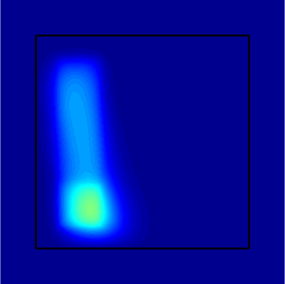
((a)) Solution at $t=0.0625$.

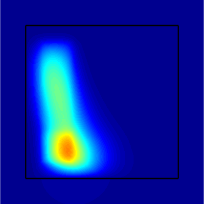
((b)) Solution at $t=0.125$.

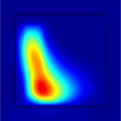
((c)) Solution at $t=0.25$.

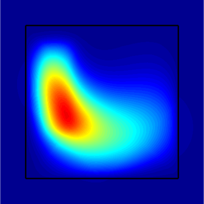
((d)) Solution at $t=0.5$.

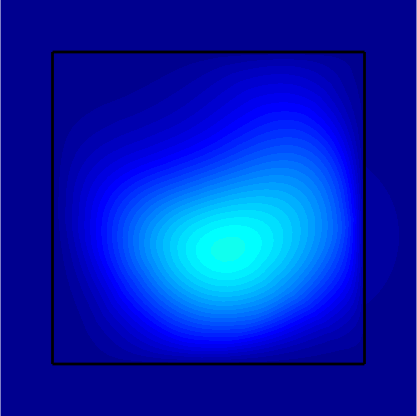
((e)) Solution at $t=0.75$.

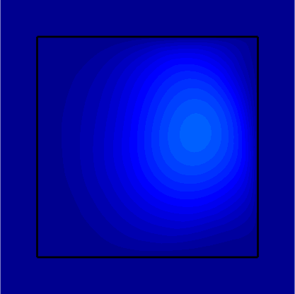
((f)) Solution at $t=1$.

Figure 3. Solution of the transport problem in section 6.3 at different times. The source is located at the left-hand side of the domain and stronger in the lower half. We turn of the source in the lower half at $t=0.25$. At $t=0.5$ the source is turned off completely.

7. Conclusions

In this paper we considered parabolic-elliptic problems, where the interior problem can be convection dominated and the exterior domain is unbounded. The coupling of the finite volume method (for the interior problem) and the boundary element method (for the exterior problem) has been proven to be a good choice for spatial discretization to handle all difficulties arising from this kind of interface problems. We showed that the semi-discrete FVM-BEM coupling yields to unique and stable solutions and converges under minimal regularity assumptions. The subsequent discretization in time by a variant of the backward Euler method yields to a fully discrete scheme that also converges under minimal regularity assumptions on the solution. As an alternative we provided a time discretization with a classical backward Euler scheme under standard regularity assumptions on the solution in the time component. Note that our analysis can also be applied for standalone FVM approximation (replace coupling conditions by boundary conditions) which improves available results in the literature.

References

• [ACF+11] M. Augustin, A. Caiazzo, A. Fiebach, J. Fuhrmann, V. John, A. Linke, and R. Umla, An assessment of discretizations for convection-dominated convection-diffusion equations, Computer Methods in Applied Mechanics and Engineering 200 (2011), no. 47, 3395 – 3409.
• [AEF+14] M. Aurada, M. Ebner, M. Feischl, S. Ferraz-Leite, T. Führer, P. Goldenits, M. Karkulik, M. Mayr, and D. Praetorius, HILBERT — a MATLAB implementation of adaptive 2D-BEM, Numer. Algor. 67 (2014), 1–32.
• [BR87] R.E. Bank and D.J. Rose, Some error estimates for the box method, SIAM J. Numer. Anal 24 (1987), 777–787.
• [Cia78] P. G. Ciarlet, The finite element method for elliptic problems, Studies in mathematics and its applications, North-Holland, Amsterdam, New-York, 1978.
• [CL99] S.-H. Chou and Q. Li, Error estimates in $L^{2}$, $H^{1}$, $L^{\infty}$ in covolume methods for elliptic and parabolic problems: a unified approach, Mathematics of Computation 69 (1999), no. 229, 103–120.
• [CLT04] P. Chatzipantelidis, R. D. Lazarov, and V. Thomée, Error estimates for a finite volume element method for parabolic equations in convex polygonal domains, Numerical Methods for Partial Differential Equations 20 (2004), no. 5, 650–674.
• [Cos88] M. Costabel, Boundary integral operators on Lipschitz domains: elementary results, SIAM J. Math. Anal. 19 (1988), 613–626.
• [EES17] H. Egger, C. Erath, and R. Schorr, On the non-symmetric coupling method for parabolic-elliptic interface problems, Preprint, arXiv:1711.08487 (2017), 1–24.
• [ELL02] R.E. Ewing, T. Lin, and Y. Lin, On the accuracy of the finite volume method based on piecewise linear polynomials, SIAM J. Numer. Anal 39 (2002), 1865–1888.
• [EOS17] C. Erath, G. Of, and F.-J. Sayas, A non-symmetric coupling of the finite volume method and the boundary element method, Numer. Math. 135 (2017), 895–922.
• [EP16] C. Erath and D. Praetorius, Adaptive vertex-centered finite volume methods with convergence rates, SIAM J. Numer. Anal. 54 (2016), no. 4, 2228–2255.
• [EP17] by same author, Céa-type quasi-optimality and convergence rates for (adaptive) vertex-centered fvm, Finite Volumes for Complex Applications VIII - Methods and Theoretical Aspects, Springer International Publishing, 2017, pp. 215–223.
• [Era10] C. Erath, Coupling of the Finite Volume Method and the Boundary Element Method - Theory, Analysis, and Numerics, Ph.D. thesis, University of Ulm, 2010.
• [Era12] by same author, Coupling of the finite volume element method and the boundary element method: an a priori convergence result, SIAM J. Numer. Anal. 50 (2012), no. 2, 574–594.
• [Era13] by same author, A new conservative numerical scheme for flow problems on unstructured grids and unbounded domains, J. Comput. Phys. 245 (2013), 476–492.
• [Eva10] L. C. Evans, Partial differential equations, Graduate studies in mathematics, American Mathematical Society, 2010.
• [Hac89] W. Hackbusch, On first and second order box schemes, Computing 41 (1989), no. 4, 277–296.
• [JN80] C. Johnson and J. C. Nédélec, On the coupling of boundary integral and finite element methods, Math. Comput. 35 (1980), 1063–1079.
• [McL00] W. McLean, Strongly elliptic systems and boundary inte gral equations, Cambridge University Press, 2000.
• [MS87] R. C. MacCamy and M. Suri, A time-dependent interface problem for two-dimensional eddy currents, Quart. Appl. Math. 44 (1987), 675–690.
• [RST08] H. G. Roos, M. Stynes, and L. Tobiska, Numerical methods for singularly perturbed differential equations, second ed., Springer, Berlin, Berlin, Heidelberg, 2008.
• [Tan14] F. Tantardini, Quasi-optimality in the backward euler-galerkin method for linear parabolic problems, Ph.D. thesis, Università degli Studi di Milano, Milan, Italy, 2014.