Distributing Complexity: A New Approach to Antenna Selection for Distributed Massive MIMO

Abstract

Antenna selection in Massive MIMO (Multiple Input Multiple Output) communication systems enables reduction of complexity, cost and power while keeping the channel capacity high and retaining the diversity, interference reduction, spatial multiplexity and array gains of Massive MIMO. We investigate the possibility of decentralised antenna selection both to parallelise the optimisation process and put the environment awareness to use. Results of experiments with two different power control rules and varying number of users show that a simple and computationally inexpensive algorithm can be used in real time. The algorithm we propose draws its foundations from self-organisation, environment awareness and randomness.

I Introduction

Combining the classical idea of antennas distributed in space [1] and the new concept of massive MIMO antenna systems [2], distributed massive MIMO offers diversity, spatial multiplexing opportunities, interference suppression and redundance [3]. The question of redundance and the number of antennas needed to operate in a certain environment can be answered under certain conditions [4], and it reinforces the importance of antenna selection. Antenna selection in Massive MIMO system can help with power optimisation, complexity reduction and provide a set of antennas available for other purposes, e.g. nulling [5]. Of course, a trade-off between these benefits exists [6] and different objectives and performance measures are used, from spectral efficiency and constructive interference [7] to fairness measures [8]. Other factors are also taken into account, such as the circuit power consumption [9]. Another aspect investigated is the difference between FDD (frequency division duplex) and TDD (time division duplex) in terms of CSI (channel state information) collection, which is essential for antenna selection [10]. These algorithms are most often centralised and based on co-located antenna systems.

A large number of antenna selection algorithms for MIMO (and recently massive MIMO) has been proposed over the last 15 years, one of the first being the removal of antennas highly correlated with other antennas in the selected set [11]. Several approaches were based on the greedy principle: in [12], the authors proposed an iterative algorithm that starts from an empty set of selected antennas and in each turn picks the antenna that contributes the most to the capacity of the selected antennas set. Its dual, i.e. the algorithm that starts with all the antennas and removes those that contribute the least iteratively, has been presented in [13]. Both algorithms terminate once the desired number of selected antennas is reached. A case for environment-ignoring random selection was made as well, pointing out that for a large number of selected antennas it is comparable to other selection procedures [14], which has been observed in practice for planar co-located massive MIMO [15]. To exemplify the various approaches used, we note that methods using convex optimisation [16], combinatorial optimisation [17], genetic algorithm [8] have been proposed.

In this letter we propose a novel distributed, local environment-aware antenna selection algorithm based on sum-capacity maximisation. The aim is to achieve sum rates comparable to those achievable through the use of more computationally complex centralised algorithms and allow flexibility and adaptability of the scheme. By distributing the computation over the nodes, we reduce computational complexity and allow the systemic complexity to enhance the performance.

II The Antenna Selection Algorithm

We consider the scenario of downlink (transmit) antenna selection at the distributed massive MIMO base station with $N_{T}$ antennas. In the cell there are $N_{R}$ single antenna users and we aim at maximising the sum-capacity

$$\mathcal{C}=\max_{\mathbf{P},\mathbf{H_{c}}}\log_{2}\det\left(\mathbf{I}+f(\rho,\,N_{TS},\,N_{R})\mathbf{H_{c}}\mathbf{P}\mathbf{H_{c}}^{H}\right)$$ (1)

where $\mathbf{I}$ is $N_{TS}\times N_{TS}$ identity matrix, $\mathbf{P}$ is a diagonal $N_{R}\times N_{R}$ matrix describing the power distribution and $\mathbf{H_{c}}$ is the $N_{TS}\times N_{R}$ channel matrix representing a selected subset of antennas from a set of $N_{T}$ antennas ($N_{T}\geq N_{TS}$) represented in the channel matrix $\mathbf{H}$, sized $N_{T}\times N_{R}$ [15]. The term $f(\rho,\,N_{TS},\,N_{R})$ represents the transmission power factor from the downlink channel model

$$\mathbf{y}=\sqrt{f(\rho,\,N_{TS},\,N_{R})}\mathbf{H_{c}z}+\mathbf{n}$$ (2)

with $\mathbf{y}$ being the $N_{R}\times 1$ received vector, $\mathbf{z}$ being the $N_{T}\times 1$ transmit vector and $\mathbf{n}$ representing the noise vector; $\rho$ is the signal to noise ratio (SNR) at each user.

There are two ways the power can be managed in downlink, and we address them both. One is harvesting the array gain by improving the SNR at the user side by taking $f(\rho,\,N_{TS},\,N_{R})=\rho N_{R}$ (power control A), while the other harvests the array gain as a means of reducing transmit power, achieved through taking $f(\rho,\,N_{TS},\>N_{R})=\rho N_{R}/N_{TS}$ (power control B). In both cases, the increase in the number of users increases the transmit power. These two optimisation problems are fundamentally different. The problem using the power control A is akin to the receiver antenna selection. This problem can be solved using greedy algorithms with a guaranteed (suboptimal) performance bound, simply adding antennas in an initially empty set of selected antennas based on the contribution to the sum rate they bring in. The problem with model B is that it is not submodular (in particular, not monotonic) [18]. This means that the addition of an antenna in the selected set of antennas can decrease channel capacity, and greedy algorithms cannot provide performance guarantees.

The optimisation problem we are solving is twofold. We are looking for both the subset of the total set of available antennas and for the optimal power distribution over them. Following the practice from [15], we initially assume all diagonal elements of $\mathbf{P}$ equal to $1/N_{R}$ (their sum is unity, making the total power equal to $f(\rho,\,N_{TS},\,N_{R})$), perform the antenna selection and then perform the selection of matrix $\mathbf{P}$ using water filling for zero forcing. The choice of zero forcing for precoding was a matter of practicality, the antenna selection algorithm we propose is independent of the channel model or the precoding scheme.

In the following explanation of the algorithm we will use the term neighbourhood for the set of $k$ elements/antenna indices denoting the $k$ nearest neighbours of an antenna ($D_{i}$: the $i$th antenna’s neighbourhood). Neighbourhood of an antenna $A$ is shown in Fig. 1. Flag bit $f_{j}$ represents the on/off state our algorithm proposes for the $j$th antenna in an iteration.

Our local algorithm is motivated by a simple model in which every antenna communicates with its neighbourhood to determine whether it should participate in the set of selected antennas $S_{i}$ from the neighbourhood $D_{i}$ or not, i.e. $S_{i}=\{j\in D_{i}|f_{j}=1\}$. Each antenna element node calculates the sum-capacity with power model B for the currently selected set of antennas from its neighbourhood, and then for this set augmented with its antenna. If the latter is larger than the former, the node sets its flag to one (else, it resets to zero).

Starting from a random selection of antennas, this simple rule in principle organises the antennas either into a stable configuration or an oscillation between two configurations. As these state(s) may be a local but not a global maximum of the achievable sum rates, we introduce a mutation flipping every ($1/p_{M}$)th flag on average. In case of long coherence intervals, the mutation happens often as the algorithm gets a chance to run longer on the same CSI. In our case, it was a rare event as we assumed a short coherence period.

The algorithm runs on the same CSI for a prescribed number of iterations $N_{i}$. After the last iteration, antennas turn on and off to form the configuration from the iteration that had the highest total capacity over all antennas. Changing the physical state of the antennas after each iteration is inefficient: this is why we work with flag bits. Size of $N_{i}$ depends on the coherence interval.

Algorithm 1 presents the self-organising behaviour we described. We dub the algorithm local to emphasise the locality of computation and perspective.

Algorithm 1 The proposed local antenna selection procedure

1. Start from a random seed of $n$ flags “on”, the rest being “off”.

2. For each antenna $i$, $1\leq i\leq N_{T}$ perform the following:

   1. Calculate the sum-capacity $\mathcal{C}_{i-}$ of the system with the channel matrix $H_{S_{i}}$ (the antennas in $S_{i}$)

   2. Calculate the sum-capacity $\mathcal{C}_{i+}$ of the system $H_{S_{i}\cup i}$

   3. Compare the two values: if $\mathcal{C}_{i+}>\mathcal{C}_{i-}$, the antenna in question should be selected (i.e. on). Otherwise it should be off.

3. Update the flags $f_{i}$ of each of the $N_{T}$ antennas to the result of 2(c) or its opposite, if a random mutation occurs (with a probability of $p_{M}$). Store the current configuration.

4. Repeat $N_{i}$ times steps 2 and 3 before updating the physical state of the antennas (on and off) to the flag state that resulted in the highest total capacity.

5. Repeat steps 2-4.

III Sum rates: Local vs. Greedy Algorithm

The algorithm was tested using raytracing Matlab tool Ilmprop [19] on a system composed by 64 antennas randomly distributed in space at the same height and shown in Fig. 1. In all computations, CSI was normalised to unit average energy over all antennas, users and subcarriers [15].

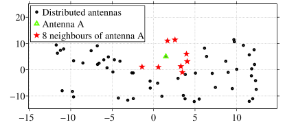
Figure 1: 64 distributed transmitters in the area which included 75 randomly distributed scatterers and one large obstacle. The number of (randomly distributed) users varied from 4 to 16. We used 300 OFDM subcarriers, SNR $\rho=-5\ \text{dB}$, 2.6 GHz carrier frequency, 20 MHz bandwidth and omnidirectional antennas for transmitters and receivers.

The two power control scenarios described before are tested and the results are shown in Fig. 2 (16 users case omitted for clarity in the second scenario plot). A clear difference between the results of local antenna selection and random selection of antennas was expected: while such a difference is often not detectable in the case of planar co-located massive MIMO, the distributed case is closer to cylindrical arrays in this sense, antennas being more far apart [15]. The curve representing the local antenna selection shows the highest sum rate values obtained for different numbers of selected antennas. It is compared with the sum rates obtained for the average random case of choosing the same numbers of antennas and the results of the previously described greedy algorithm (the one starting with an empty set of antennas [12]). The sum rates obtained through the proposed local algorithm are on par (even marginally better) as those obtained through the greedy algorithm (very low antenna counts for which our algorithm gives zero rates are not relevant, as they are within $N_{TS}\lesssim N_{R}$ range, not enabling proper beamforming for all users). The proposed local selection mechanism achieves a comparable performance to the greedy selection, while reducing the computational complexity.

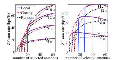
Figure 2: Antenna selection effects on ZF sum rate for different number of users in scenarios with power control A and B

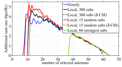
Figure 3: ZF sum rate for different antenna selection algorithms in 8 users case with power control A represented as the additional sum rate with respect to random selection. $\delta$CSI: variation of 30% in imperfect CSI measurement.

IV Computational and Systemic Complexity

IV-A Computational Complexity

Theorem 1.

The worst case complexity of the proposed algorithm is $\mathcal{O}(N_{T}^{\omega})$, where $\omega$, $2<\omega<3$ is the exponent in the employed matrix multiplication algorithm complexity..

Proof:

We first note that $\det(\mathbf{I}+\mathbf{AB})=\det(\mathbf{I}+\mathbf{BA})$ for properly sized identity matrices $\mathbf{I}$ on both sides (Sylvester identity), so we can shift from $N_{T}\times N_{T}$ matrix $\mathbf{H}\mathbf{H}^{H}$ to a smaller $N_{R}\times N_{R}$ matrix $\mathbf{H}^{H}\mathbf{H}$. The total number of matrix multiplications is $2N_{i}$ and they would be conducted using some of the standard algorithms with complexity $\mathcal{O}(N_{R}^{\omega-1}N_{T})$, $2<\omega<3$ [20]. This brings the multiplication complexity of our algorithm to $\mathcal{O}(N_{i}N_{R}^{\omega-1}N_{T})$. In the worst case $N_{R}=N_{T}$, and since $N_{i}=\text{const}$ we obtain the complexity of $\mathcal{O}(N_{T}^{\omega})$. The number of determinant calculations is constant ($\mathcal{O}(N_{i})$), so the overall complexity is $\mathcal{O}(N_{T}^{\omega})$. ∎

Comparing this to the case of the greedy algorithms with complexity $\mathcal{O}(N_{T}^{2}N_{R}^{2})$ [13] and $\mathcal{O}(N_{T}N_{R}N_{TS})$ [12], we see that the complexity is reduced: the effect is best seen for a large number of antennas (massive MIMO) where the constant nature of $N_{i}$ enables efficient scaling. We also note that $N_{R}$ and $N_{T}$ in our algorithm consideration are not the entire set of transmitters and receivers as in the greedy algorithms, but just a $k$-neighbourhood of transmitters and the receivers in their vicinity. Hence, the computational complexity decreases even more in the practical implementation.

The main computational burden of the single iteration of both algorithms is the fact that it is repeated for each of the $c$ OFDM subcarriers. A natural question to ask is whether we need to optimise over the whole set of subcarriers, and if a significantly smaller subset could be selected to represent the channel appropriately. In our study we propose a random selection of a subcarrier subset and argue that 5% of the whole set is enough for practical use, based on the results. This approach gives a good representation of the channel for the algorithm as the procedure is repeated $N_{i}$ times, allowing most of the subcarriers to appear in different iterations and influence the antenna selection. The alternative is selecting a fixed number of the subcarriers with the largest average power over all users. Using any subset of subcarriers could also speed up the greedy algorithm, but our local selection algorithm still has lower complexity. Fig. 3 represents the gain of sum capacity over random antenna selection for eight users scenario where we compare the results of greedy selection and three local algorithm variants: the original proposal using all 300 subcarriers, one with 15 randomly selected subcarriers and one with 60 strongest subcarriers selected. The random subcarrier selection variant is computationally superior to both alternatives. It is marginally better in terms of sum rates and we can observe from Fig. 3 that its minimum selection sets are in general smaller than those of the full 300 subcarrier algorithm. The strongest subset-based variant a limited applicability due to a large minimum number of selected antennas.

Another issue with the growing complexity is the collection of CSI. It is unrealistic to expect perfect knowledge of CSI, but as Fig. 3 shows, it is not necessary: a 30% uncertainty in CSI hs negligible impact on the result of antenna selection.

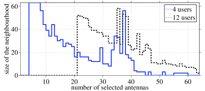
Figure 4: The relationship between the number of selected antennas and the number of neighbours taken in the algorithm

IV-B Systemic Complexity: Self-Organisation

Our algorithm does not start with a predefined number of antennas to be selected, but converges to a subset whose size depends on the size of the neighbourhood. This means that for the comparison with the greedy algorithm shown in Figs. 2 and 3 we have run the algorithm for varying numbers of neighbours considered. Fig. 4 shows the size of the neighbourhood observed and the number of selected antennas in each of those cases for scenarios with 4 and 12 users (the other two scenarios omitted for clarity) in the power control scheme A. The variable parameter is placed on the ordinate axis to align the graph with Fig. 2.

The figure demonstrates that the smallest number of antennas is selected in the case when a single antenna sees most of the other antennas as its neighbours, and vice versa, the largest number of antennas is selected in correspondence to the smallest neighbourhoods. Small neighbourhoods make large effort to support all users, hence turning on most of their antennas, leading to a high total count of selected antennas. In large neighbourhoods suboptimal antennas keep themselves out of the selected subset, seeing the better antennas already in. We also note the characteristic bimodal shape, implying that in large neighbourhoods the algorithm switches (oscillates) between small number of selected antennas and roughly 50% of the total number. This is a consequence of the power control B we use (cf. the location of maxima of the sum rates in Fig. 2(b)) as roughly half of the antennas do not contribute anything new once the other antennas are included in the selected set. In large neighbourhoods, entropy is low as all antennas know how they fare against other antennas, making them more aware of the environment and the rest of the system.

Figs. 2 and 4 also show that the minimal number of selected antennas is not always the number of users: the algorithm sometimes adds more antennas for better beamforming.

V Conclusions

We have presented a novel local antenna selection method for distributed massive MIMO. Its local nature allows it to be environment-aware and enables distributed computing at every node. While reducing the complexity of matrix operations and distributing it over all antenna nodes, we have additionaly reduced computational complexity by using a very small subset of subcarriers for optimisation, reducing the time cost by 20 times. This reduction resulted in both enabling the real-time application of the algorithm in dynamic environments with short coherence time and retaining sum-rates on par with other antenna selection algorithms.

Relying on self-organisation, this algorithm emphasises the local properties of distributed massive MIMO and supports its modularity, namely the option of cluster separation and distributed control. The distributed control aspect allows user selection aided by our algorithm for users close to a neighbourhood cluster, and also the service consolidation in case of device failures within a cluster. The neighbouring antennas are aware of local faults and organise themselves accordingly in an emergent manner, building up on the inherent systemic complexity of the antenna selection algorithm. The clusters may operate on their own and/or interact with other clusters, depending on the set neighbourhood size.

The local selection algorithm relies on randomness in two ways. Randomly selecting subcarriers to do the optimisation on, it keeps the diversity of the full subcarrier set while reducing computation time. Randomly performing mutations on state transitions, it allows leaving local maxima.

The reduced computational complexity and environment awareness enable a flexible real time application. Being independent from precoding choice, channel model and the form of power control, the algorithm has been shown to perform well in two different variants of transmit antenna selection.

References

- [1] K. J. Kerpez. A radio access system with distributed antennas. IEEE Transactions on Vehicular Technology, 45(2):265–275, 1996.
- [2] T. L. Marzetta. Noncooperative Cellular Wireless with Unlimited Numbers of Base Station Antennas. IEEE Transactions on Wireless Communications, 9(11):3590–3600, November 2010.
- [3] A. Ozgur, O. Lévêque, and D. Tse. Spatial degrees of freedom of large distributed mimo systems and wireless ad hoc networks. IEEE Journal on Selected Areas in Communications, 31(2):202–214, 2013.
- [4] J. Hoydis, S. ten Brink, and M. Debbah. Massive MIMO in the UL/DL of Cellular Networks: How Many Antennas Do We Need? IEEE Journal on Selected Areas in Communications, 31(2):160–171, February 2013.
- [5] G. Geraci, A. Garcia-Rodriguez, D. Lopez-Perez, A. Bonfante, L. Galati Giordano, and H. Claussen. Operating Massive MIMO in Unlicensed Bands for Enhanced Coexistence and Spatial Reuse. IEEE Journal on Selected Areas in Communications, 35(6):1282–1293, June 2017.
- [6] Z. Liu, W. Du, and D. Sun. Energy and Spectral Efficiency Tradeoff for Massive MIMO Systems With Transmit Antenna Selection. IEEE Transactions on Vehicular Technology, 66(5):4453–4457, May 2017.
- [7] P. V. Amadori and C. Masouros. Interference-Driven Antenna Selection for Massive Multiuser MIMO. IEEE Transactions on Vehicular Technology, 65(8):5944–5958, August 2016.
- [8] B. Makki, A. Ide, T. Svensson, T. Eriksson, and M. S. Alouini. A Genetic Algorithm-Based Antenna Selection Approach for Large-but-Finite MIMO Networks. IEEE Transactions on Vehicular Technology, 66(7):6591–6595, July 2017.
- [9] R. Hamdi, E. Driouch, and W. Ajib. Resource Allocation in Downlink Large-Scale MIMO Systems. IEEE Access, 4:8303–8316, 2016.
- [10] M. Benmimoune, E. Driouch, W. Ajib, and D. Massicotte. Novel transmit antenna selection strategy for massive MIMO downlink channel. Wireless Networks, 23(8):2473–2484, November 2017.
- [11] A. F. Molisch, M. Z. Win, Yang-Seok Choi, and J. H. Winters. Capacity of MIMO systems with antenna selection. IEEE Transactions on Wireless Communications, 4(4):1759–1772, July 2005.
- [12] M. Gharavi-Alkhansari and A. B. Gershman. Fast antenna subset selection in MIMO systems. IEEE Transactions on Signal Processing, 52(2):339–347, February 2004.
- [13] A. Gorokhov, D. A. Gore, and A. J. Paulraj. Receive antenna selection for MIMO spatial multiplexing: theory and algorithms. IEEE Transactions on Signal Processing, 51(11):2796–2807, November 2003.
- [14] B. M. Lee, J. Choi, J. Bang, and B. C. Kang. An energy efficient antenna selection for large scale green MIMO systems. In 2013 IEEE International Symposium on Circuits and Systems (ISCAS2013), pages 950–953, May 2013.
- [15] X. Gao, O. Edfors, F. Tufvesson, and E. G. Larsson. Massive MIMO in Real Propagation Environments: Do All Antennas Contribute Equally? IEEE Transactions on Communications, 63(11):3917–3928, 2015.
- [16] S. Mahboob, R. Ruby, and V. C. M. Leung. Transmit Antenna Selection for Downlink Transmission in a Massively Distributed Antenna System Using Convex Optimization. In 2012 Seventh International Conference on Broadband, Wireless Computing, Communication and Applications, pages 228–233, November 2012.
- [17] D. S. Michalopoulos, G. K. Karagiannidis, T. A. Tsiftsis, and R. K. Mallik. Distributed Transmit Antenna Selection (DTAS) Under Performance or Energy Consumption Constraints. IEEE Transactions on Wireless Communications, 7(4):1168–1173, April 2008.
- [18] R. Vaze and H. Ganapathy. Sub-Modularity and Antenna Selection in MIMO Systems. IEEE Communications Letters, 16(9):1446–1449, September 2012.
- [19] G Del Galdo, M Haardt, and C Schneider. Geometry-based channel modelling of mimo channels in comparison with channel sounder measurements. Advances in Radio Science, 2(BC):117–126, 2005.
- [20] P. A. Knight. Fast rectangular matrix multiplication and qr decomposition. Linear algebra and its applications, 221:69–81, 1995.