Multi-Agent Path Finding with Deadlines: Preliminary Results

Abstract.

We formalize the problem of multi-agent path finding with deadlines (MAPF-DL). The objective is to maximize the number of agents that can reach their given goal vertices from their given start vertices within a given deadline, without colliding with each other. We first show that the MAPF-DL problem is NP-hard to solve optimally. We then present an optimal MAPF-DL algorithm based on a reduction of the MAPF-DL problem to a flow problem and a subsequent compact integer linear programming formulation of the resulting reduced abstracted multi-commodity flow network.

1. Introduction

Multi-agent path finding (MAPF) is the problem of planning collision-free paths for multiple agents in known environments from their given start vertices to their given goal vertices. MAPF is important, for example, for aircraft-towing vehicles Morris et al. (2016), warehouse and office robots Wurman et al. (2008); Veloso et al. (2015), and game characters Ma et al. (2017). The objective is to minimize the sum of the arrival times of the agents or the makespan. The MAPF problem is NP-hard to solve optimally Yu and LaValle (2013b) and even to approximate within a small constant factor for makespan minimization Ma et al. (2016). It can be solved with reductions to other well-studied combinatorial problems Surynek (2015); Yu and LaValle (2013a); Erdem et al. (2013); Nguyen et al. (2017) and dedicated optimal Standley (2010); Standley and Korf (2011); Goldenberg et al. (2014); Sharon et al. (2013); Wagner and Choset (2015); Sharon et al. (2015); Boyarski et al. (2015); Felner et al. (2018), bounded-suboptimal Barer et al. (2014); Cohen et al. (2016), and suboptimal MAPF algorithms Silver (2005); Sturtevant and Buro (2006); Wang and Botea (2011); Luna and Bekris (2011); de Wilde et al. (2013); Wagner and Choset (2011), as described in several surveys Ma et al. (2016); Felner et al. (2017).

The MAPF problem has recently been generalized in different directions Ma and Koenig (2016); Hönig et al. (2016a); Ma et al. (2016); Hönig et al. (2016b); Ma et al. (2017a, b); Ma et al. (2017) but none of them capture an important characteristic of many applications, namely the ability to meet deadlines. We thus formalize the multi-agent path finding problem with deadlines (MAPF-DL problem). The objective is to maximize the number of agents that can reach their given goal vertices from their given start vertices within a given deadline, without colliding with each other. In previously studied MAPF problems, all agents have to be routed from their start vertices to their goal vertices, and the objective is with regard to resources such as fuel (sum of arrival times) or time (makespan). In the MAPF-DL problem, on the other hand, the resources are the agents themselves. We first show that the MAPF-DL problem is NP-hard to solve optimally. We then present an optimal MAPF-DL algorithm based on a reduction of the MAPF-DL problem to a flow problem and a subsequent compact integer linear programming formulation of the resulting reduced abstracted multi-commodity flow network.

2. MAPF-DL Problem

We formalize the MAPF-DL problem as follows: We are given a deadline, denoted by a time step $T_{end}$, an undirected graph $G=(V,E)$, and $M$ agents $a_{1},a_{2}\ldots a_{M}$. Each agent $a_{i}$ has a start vertex $s_{i}$ and a goal vertex $g_{i}$. In each time step, each agent either moves to an adjacent vertex or stays at the same vertex. Let $l_{i}(t)$ be the vertex occupied by agent $a_{i}$ at time step $t\in\{0\ldots T_{end}\}$. Call an agent $a_{i}$ successful iff it occupies its goal vertex at the deadline $T_{end}$, that is, $l_{i}(T_{end})=g_{i}$. A plan consists of a path $l_{i}$ assigned to each successful agent $a_{i}$. Unsuccessful agents are removed at time step zero and thus have no paths assigned to them. A solution is a plan that satisfies the following conditions: (1) For all successful agents $a_{i}$, $l_{i}(0)=s_{i}$ [each successful agent starts at its start vertex]. (2) For all successful agents $a_{i}$ and all time steps $t>0$, $(l_{i}(t-1),l_{i}(t))\in E$ or $l_{i}(t-1)=l_{i}(t)$ [each successful agent always either moves to an adjacent vertex or does not move]. (3) For all pairs of different successful agents $a_{i}$ and $a_{j}$ and all time steps $t$, $l_{i}(t)\neq l_{j}(t)$ [two successful agents never occupy the same vertex simultaneously]. (4) For all pairs of different successful agents $a_{i}$ and $a_{j}$ and all time steps $t>0$, $l_{i}(t-1)\neq l_{j}(t)$ or $l_{j}(t-1)\neq l_{i}(t)$ [two successful agents never traverse the same edge simultaneously in opposite directions]. Define a collision between two different successful agents $a_{i}$ and $a_{j}$ to be either a vertex collision ($a_{i}$, $a_{j}$, $v$, $t$) iff $v=l_{i}(t)=l_{j}(t)$ (corresponding to Condition 3) or an edge collision ($a_{i}$, $a_{j}$, $u$, $v$, $t$) iff $u=l_{i}(t)=l_{j}(t+1)$ and $v=l_{j}(t)=l_{i}(t+1)$ (corresponding to Condition 4). The objective is to maximize the number of successful agents $M_{succ}=\left|\{a_{i}|l_{i}(T_{end})=g_{i}\}\right|$.

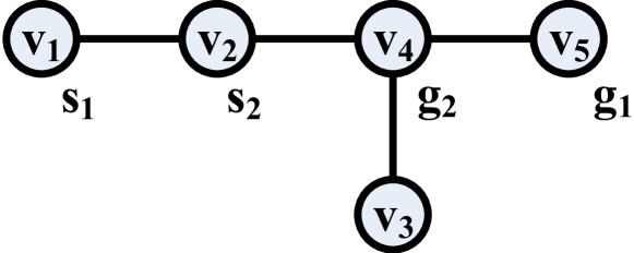
(a)

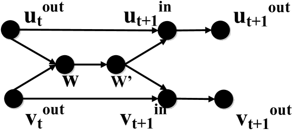
(b)

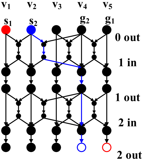
(c)

Figure 1. (a) Running example of a MAPF-DL instance. (b) Construction for edge $(u,v)\in E$ between time steps $t$ and $t+1$. (c) Flow network for the running example.

Theorem 1.

It is NP-hard to compute a MAPF-DL solution with the maximum number of successful agents.

The proof of the theorem reduces the $\bm{\leq}$3,$\bm{=}$3-SAT problem Tovey (1984), an NP-complete version of the Boolean satisfiability problem, to the MAPF-DL problem. The reduction is similar to the one used for proving the NP-hardness of approximating the optimal makespan for the MAPF problem Ma et al. (2016). It constructs a MAPF-DL instance with deadline $T_{end}=3$ that has a solution where all agents are successful iff the given $\bm{\leq}$3,$\bm{=}$3-SAT instance is satisfiable.

3. Optimal MAPF-DL Algorithm

Our optimal MAPF-DL algorithm first reduces the MAPF-DL problem to the maximum (integer) multi-commodity flow problem, which is similar to the reductions of the MAPF and TAPF problems to multi-commodity flow problems Yu and LaValle (2013a); Ma and Koenig (2016): Given a MAPF-DL instance with deadline $T_{end}$, we construct a multi-commodity flow network $\mathcal{N}=(\mathcal{V},\mathcal{E})$ with vertices $\mathcal{V}=\bigcup_{v\in V}(\{v_{0}^{out}\}\cup\bigcup_{t=1}^{T_{end}}\{v_{t}^{in},v_{t}^{out}\})$ and directed edges $\mathcal{E}$ with unit capacity. The vertices $v_{t}^{out}$ represent vertex $v\in V$ at the end of time step $t$ and the beginning of time step $t+1$, while the vertices $v_{t}^{in}$ are intermediate vertices. For each agent $a_{i}$, we set a supply of one at (start) vertex $(s_{i})_{0}^{out}$ and a demand of one at (goal) vertex $(g_{i})^{out}_{T_{end}}$, both for commodity type $i$ (corresponding to agent $a_{i}$). For each time step, we construct the gadgets shown in Figure 1(b) to prevent vertex and edge collisions. The objective is to maximize the total amount of integral flow received in all vertices $(g_{i})^{out}_{T_{end}}$, which can be achieved via a standard integer linear programming (ILP) formulation.

Theorem 2.

There is a one-to-one correspondence between all solutions of a MAPF-DL instance with the maximum number of successful agents and all maximum integral flows on the corresponding flow network.

The proof of the theorem is similar to the one for the reduction of the MAPF problem to the multi-commodity flow problem Yu and LaValle (2013a).

Figure 1(a) shows a MAPF-DL instance with deadline $T_{end}=2$. Agents $a_{1}$ and $a_{2}$ have start vertices $s_{1}$ and $s_{2}$ and goal vertices $g_{1}$ and $g_{2}$, respectively. The number of successful agents is at most $M_{succ}=1$ because only agent $a_{2}$ can reach its goal vertex in two time steps. Figure 1(c) shows the corresponding flow network with a maximum flow (in color) that corresponds to a solution with unsuccessful agent $a_{1}$ and successful agent $a_{2}$ with path $\langle v_{2}$, $v_{4}$, $v_{4}\rangle$.

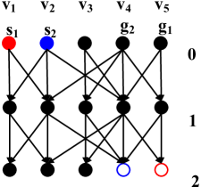
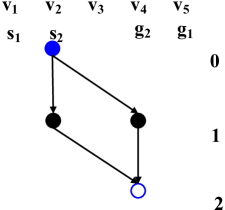
Figure 2. Optimization for the running example. Left: Abstracted flow network. Right: Reduced abstracted flow network.

Abstracted Flow Network and Compact ILP Formulation We construct a compact ILP formulation based on an abstraction of the flow network $\mathcal{N}=(\mathcal{V},\mathcal{E})$ and additional linear constraints to prevent vertex and edge collisions. We obtain the abstracted flow network $\mathcal{N^{\prime}}=(\mathcal{V^{\prime}},\mathcal{E^{\prime}})$ by (1) contracting each $(v_{t}^{in},v_{t}^{out})\in\mathcal{E}$ and replacing $v_{t}^{in}$ and $v_{t}^{out}$ with a single vertex $v_{t}$ for all $v\in V$ and $t=1\ldots T_{end}$ (and $v_{0}^{out}$ with $v_{0}$); and (2) replacing the gadget for each $(u,v)\in E$ and each $t=0\ldots T_{end}-1$ with a pair of edges $(u_{t},v_{t+1})$ and $(v_{t},u_{t+1})$. Figure 2 (left) shows an example. Then, we use the standard ILP formulation of this abstracted network augmented with the constraints shown in red:

$$\text{maximize }M_{succ}=\sum_{i=1\ldots M}\sum_{e\in\delta^{-}((s_{i})_{0})}x_{i}[e]\text{, subject to}$$

$$0\leq\sum_{i=1}^{M}x_{i}[e]\leq 1\quad e\in\mathcal{E^{\prime}}\quad\text{(subsumed by the top red constraints)}$$

$$\sum_{e\in\delta^{+}(v)}x_{i}[e]-\sum_{e\in\delta^{-}(v)}x_{i}[e]=0\quad i=1\ldots M,v\in\mathcal{V^{\prime}}\setminus\{(s_{i})_{0},(g_{i})_{T_{end}}\}$$

$$\sum_{e\in\delta^{-}((s_{i})_{0})}x_{i}[e]=\sum_{e\in\delta^{+}((g_{i})_{T_{end}})}x_{i}[e]\quad i=1\ldots M$$

$$\color[rgb]{1,0,0}\sum_{i=1\ldots M}\sum_{e\in\delta^{-}(v)}x_{i}[e]\leq 1\quad v\in\mathcal{V^{\prime}}$$

$$\color[rgb]{1,0,0}\sum_{i=1\ldots M}x_{i}[(u_{t},v_{t+1})]+\sum_{i=1\ldots M}x_{i}[(v_{t},u_{t+1})]\leq 1\quad(u_{t},v_{t+1}),\leavevmode\nobreak\ (v_{t},u_{t+1})\in\mathcal{E^{\prime}},$$

where the 0/1 variable $x_{i}[e]$ represents the amount of flow of commodity type $i$ on edge $e\in\mathcal{E^{\prime}}$ and the sets $\delta^{-}(v)$ and $\delta^{+}(v)$ contain all outgoing and incoming, respectively, edges of vertex $v$. The top red constraints prevent vertex collisions of the form $(*,*,v,t)$, and the bottom red constraints prevent edge collisions of the forms $(*,*,u,v,t)$ and $(*,*,v,u,t)$.

Reduced Abstracted Flow Network We can remove all vertices and edges from the abstracted flow network that are not on some path from at least one start vertex to the corresponding goal vertex in the abstracted flow network. This can be done by performing one complete forward breadth-first search from each start vertex and one complete backward breadth-first search from each goal vertex and then keeping only those vertices and edges that are part of the search trees associated with at least one start vertex and the corresponding goal vertex. Figure 2 (right) shows an example. We then use the compact ILP formulation of the resulting reduced abstracted flow network.

Experimental Evaluation We tested our optimal MAPF-DL algorithm on a 2.50 GHz Intel Core i5-2450M laptop with 6 GB RAM, using CPLEX V12.7.1 IBM (2011) as the ILP solver. We randomly generated MAPF-DL instances with different numbers of agents (ranging from 10 to 100 in increments of 10) on $40\times 40$ 4-neighbor 2D grids with deadline $T_{end}=$ 50. We blocked all grid cells independently at random with 20% probability each. We generated 50 MAPF-DL instances for each number of agents. We placed the start and goal vertices of each agent randomly at distance 48, 49, or 50. The following table shows the percentage of instances that could be solved within a runtime limit of 60 seconds per instance.

agents	10	20	30	40	50	60	70	80	90	100
success rate	100%	100%	100%	100%	98%	88%	50%	12%	0%	0%

References

- (1)
- Barer et al. (2014) M. Barer, G. Sharon, R. Stern, and A. Felner. 2014. Suboptimal Variants of the Conflict-Based Search Algorithm for the Multi-Agent Pathfinding Problem. In SoCS. 19–27.
- Boyarski et al. (2015) E. Boyarski, A. Felner, R. Stern, G. Sharon, D. Tolpin, O. Betzalel, and S. E. Shimony. 2015. ICBS: Improved Conflict-Based Search Algorithm for Multi-Agent Pathfinding. In IJCAI. 740–746.
- Cohen et al. (2016) L. Cohen, T. Uras, T. K. S. Kumar, H. Xu, N. Ayanian, and S. Koenig. 2016. Improved Solvers for Bounded-Suboptimal Multi-Agent Path Finding. In IJCAI. 3067–3074.
- de Wilde et al. (2013) B. de Wilde, A. W. ter Mors, and C. Witteveen. 2013. Push and Rotate: Cooperative Multi-Agent Path Planning. In AAMAS. 87–94.
- Erdem et al. (2013) E. Erdem, D. G. Kisa, U. Oztok, and P. Schueller. 2013. A General Formal Framework for Pathfinding Problems with Multiple Agents. In AAAI. 290–296.
- Felner et al. (2018) A. Felner, J. Li, E. Boyarski, H. Ma, L. Cohen, T. K. S. Kumar, and S. Koenig. 2018. Adding Heuristics to Conflict-Based Search for Multi-Agent Path Finding. ICAPS (2018).
- Felner et al. (2017) A. Felner, R. Stern, S. E. Shimony, E. Boyarski, M. Goldenberg, G. Sharon, N. R. Sturtevant, G. Wagner, and P. Surynek. 2017. Search-Based Optimal Solvers for the Multi-Agent Pathfinding Problem: Summary and Challenges. In SoCS. 29–37.
- Goldenberg et al. (2014) M. Goldenberg, A. Felner, R. Stern, G. Sharon, N. R. Sturtevant, R. C. Holte, and J. Schaeffer. 2014. Enhanced Partial Expansion A*. Journal of Artificial Intelligence Research 50 (2014), 141–187.
- Hönig et al. (2016a) W. Hönig, T. K. S. Kumar, L. Cohen, H. Ma, H. Xu, N. Ayanian, and S. Koenig. 2016a. Multi-Agent Path Finding with Kinematic Constraints. In ICAPS. 477–485.
- Hönig et al. (2016b) W. Hönig, T. K. S. Kumar, H. Ma, N. Ayanian, and S. Koenig. 2016b. Formation Change for Robot Groups in Occluded Environments. In IROS. 4836–4842.
- IBM (2011) IBM. 2011. IBM ILOG CPLEX Optimization Studio CPLEX User’s Manual.
- Luna and Bekris (2011) R. Luna and K. E. Bekris. 2011. Push and Swap: Fast Cooperative Path-Finding with Completeness Guarantees. In IJCAI. 294–300.
- Ma et al. (2017) H. Ma, W. Hönig, L. Cohen, T. Uras, H. Xu, T. K. S. Kumar, N. Ayanian, and S. Koenig. 2017. Overview: A Hierarchical Framework for Plan Generation and Execution in Multi-Robot Systems. IEEE Intelligent Systems 32, 6 (2017), 6–12.
- Ma and Koenig (2016) H. Ma and S. Koenig. 2016. Optimal Target Assignment and Path Finding for Teams of Agents. In AAMAS. 1144–1152.
- Ma et al. (2016) H. Ma, S. Koenig, N. Ayanian, L. Cohen, W. Hönig, T. K. S. Kumar, T. Uras, H. Xu, C. Tovey, and G. Sharon. 2016. Overview: Generalizations of Multi-Agent Path Finding to Real-World Scenarios. In IJCAI-16 Workshop on Multi-Agent Path Finding.
- Ma et al. (2017a) H. Ma, T. K. S. Kumar, and S. Koenig. 2017a. Multi-Agent Path Finding with Delay Probabilities. In AAAI. 3605–3612.
- Ma et al. (2017b) H. Ma, J. Li, T. K. S. Kumar, and S. Koenig. 2017b. Lifelong Multi-Agent Path Finding for Online Pickup and Delivery Tasks. In AAMAS. 837–845.
- Ma et al. (2016) H. Ma, C. Tovey, G. Sharon, T. K. S. Kumar, and S. Koenig. 2016. Multi-Agent Path Finding with Payload Transfers and the Package-Exchange Robot-Routing Problem. In AAAI. 3166–3173.
- Ma et al. (2017) H. Ma, J. Yang, L. Cohen, T. K. S. Kumar, and S. Koenig. 2017. Feasibility Study: Moving Non-Homogeneous Teams in Congested Video Game Environments. In AIIDE. 270–272.
- Morris et al. (2016) R. Morris, C. Pasareanu, K. Luckow, W. Malik, H. Ma, S. Kumar, and S. Koenig. 2016. Planning, Scheduling and Monitoring for Airport Surface Operations. In AAAI-16 Workshop on Planning for Hybrid Systems.
- Nguyen et al. (2017) V. Nguyen, P. Obermeier, T. C. Son, T. Schaub, and W. Yeoh. 2017. Generalized Target Assignment and Path Finding Using Answer Set Programming. In IJCAI. 1216–1223.
- Sharon et al. (2015) G. Sharon, R. Stern, A. Felner, and N. R. Sturtevant. 2015. Conflict-Based Search for Optimal Multi-Agent Pathfinding. Artificial Intelligence 219 (2015), 40–66.
- Sharon et al. (2013) G. Sharon, R. Stern, M. Goldenberg, and A. Felner. 2013. The Increasing Cost Tree Search for Optimal Multi-Agent Pathfinding. Artificial Intelligence 195 (2013), 470–495.
- Silver (2005) D. Silver. 2005. Cooperative Pathfinding. In AIIDE. 117–122.
- Standley (2010) T. S. Standley. 2010. Finding Optimal Solutions to Cooperative Pathfinding Problems. In AAAI. 173–178.
- Standley and Korf (2011) T. S. Standley and R. E. Korf. 2011. Complete Algorithms for Cooperative Pathfinding Problems. In IJCAI. 668–673.
- Sturtevant and Buro (2006) N. R. Sturtevant and M. Buro. 2006. Improving Collaborative Pathfinding Using Map Abstraction. In AIIDE. 80–85.
- Surynek (2015) P. Surynek. 2015. Reduced Time-Expansion Graphs and Goal Decomposition for Solving Cooperative Path Finding Sub-Optimally. In IJCAI. 1916–1922.
- Tovey (1984) C. A. Tovey. 1984. A Simplified NP-Complete Satisfiability Problem. Discrete Applied Mathematics 8 (1984), 85–90.
- Veloso et al. (2015) M. Veloso, J. Biswas, B. Coltin, and S. Rosenthal. 2015. CoBots: Robust Symbiotic Autonomous Mobile Service Robots. In IJCAI. 4423–4429.
- Wagner and Choset (2011) G. Wagner and H. Choset. 2011. M*: A Complete Multirobot Path Planning Algorithm with Performance Bounds. In IROS. 3260–3267.
- Wagner and Choset (2015) G. Wagner and H. Choset. 2015. Subdimensional Expansion for Multirobot Path Planning. Artificial Intelligence 219 (2015), 1–24.
- Wang and Botea (2011) K. Wang and A. Botea. 2011. MAPP: A Scalable Multi-Agent Path Planning Algorithm with Tractability and Completeness Guarantees. Journal of Artificial Intelligence Research 42 (2011), 55–90.
- Wurman et al. (2008) P. R. Wurman, R. D’Andrea, and M. Mountz. 2008. Coordinating Hundreds of Cooperative, Autonomous Vehicles in Warehouses. AI Magazine 29, 1 (2008), 9–20.
- Yu and LaValle (2013a) J. Yu and S. M. LaValle. 2013a. Planning Optimal Paths for Multiple Robots on Graphs. In ICRA. 3612–3617.
- Yu and LaValle (2013b) J. Yu and S. M. LaValle. 2013b. Structure and Intractability of Optimal Multi-Robot Path Planning on Graphs. In AAAI. 1444–1449.