The Green Bank North Celestial Cap Pulsar Survey III: 45 New Pulsar Timing Solutions

Abstract

We provide timing solutions for 45 radio pulsars discovered by the Robert C. Byrd Green Bank Telescope. These pulsars were found in the Green Bank North Celestial Cap pulsar survey, an all-GBT-sky survey being carried out at a frequency of $350\;\textrm{MHz}$. We include pulsar timing data from the Green Bank Telescope and Low Frequency Array. Our sample includes five fully recycled millisecond pulsars (MSPs, three of which are in a binary system), a new relativistic double neutron star system, an intermediate mass binary pulsar, a mode-changing pulsar, a 138-ms pulsar with a very low magnetic field, and several nulling pulsars. We have measured two post-Keplerian parameters and thus the masses of both objects in the double neutron star system. We also report a tentative companion mass measurement via Shapiro delay in a binary MSP. Two of the MSPs can be timed with high precision and have been included in pulsar timing arrays being used to search for low-frequency gravitational waves, while a third MSP is a member of the black widow class of binaries. Proper motion is measurable in five pulsars and we provide an estimate of their space velocity. We report on an optical counterpart to a new black widow system and provide constraints on the optical counterparts to other binary MSPs. We also present a preliminary analysis of nulling pulsars in our sample. These results demonstrate the scientific return of long timing campaigns on pulsars of all types.

1 Introduction

Radio pulsars have long been used as exquisite natural laboratories for studying a wide range of phenomena in physics and astronomy. The well known double neutron star system PSR B1913+16 provided the first observational evidence for the existence of gravitational waves (GWs, Taylor & Weisberg, 1989; Weisberg et al., 2010), and the double pulsar system J0737$-$3039 continues to place ever more stringent constraints on deviations from general relativity (GR) in the strong-field regime (Kramer et al., 2006). Neutron star mass measurements can be used to study nuclear physics and the equation-of-state of ultra-dense matter (Demorest et al., 2010), while also providing insight into the mass distribution of the neutron star population (Özel et al., 2012; Kiziltan et al., 2013; Antoniadis et al., 2016) and in turn formation mechanisms and evolution (e.g. Lattimer & Prakash, 2004; Tauris & Savonije, 1999). Proper motion measurements can be used to estimate transverse velocity, which also informs theories of neutron star formation and supernovae energetics (Ferdman et al., 2013). While most binary pulsars have low-mass He white dwarf (WD) companions, rarer binaries have also been found. These include systems with more massive CO WDs (e.g. Camilo et al., 2001), giant companions that are actively transferring mass to the neutron star, and so-called black widow binaries where an energetic pulsar wind has ablated the companion’s outer layers, leaving a very low-mass degenerate core (Roberts, 2013).

High-precision millisecond pulsars (MSP, which we define as $P<10\;\textrm{ms}$) are currently being used in an effort to directly detect nanohertz frequency GWs by forming a pulsar timing array (PTA). GWs are predicted to cause nanosecond-scale deviations in pulse arrival times with a unique angular correlation between pairs of MSPs. At nanohertz frequencies the dominant source class is expected to be supermassive binary black holes in the early stages of inspiral, though more exotic sources such as cosmic strings are also predicted to emit at these GW frequencies. One of the best ways to improve the sensitivity of PTAs is by adding new high-precision pulsars to the array, particularly on angular baselines that are not currently well sampled (Siemens et al., 2013). PTAs are a major project at all large radio telescopes: the North American Nanohertz Observatory for Gravitational Waves (NANOGrav; McLaughlin 2013) uses the Robert C. Byrd Green Bank Telescope (GBT) and William E. Gordon telescope at the Arecibo Observatory, the Parkes Pulsar Timing Array (PPTA; Hobbs 2013) uses the Parkes Telescope, and the European Pulsar Timing Array (EPTA; Kramer & Champion 2013) uses the Effelsberg Telescope, the Lovell Telescope, the Nançay Radio Telescope, the Sardinia Radio Telescope, and the Westerbork Synthesis Array. All of these projects also collaborate under the framework of the International Pulsar Timing Array (Manchester & IPTA, 2013).

Despite many decades of investigation, pulsar emission mechanisms are not fully understood. A wide variety of behavior is observed, however. This includes abrupt changes in the average pulse profile between a small number of modes that may be accompanied by changes in the spin-down rate of the pulsar and are tied to global magnetospheric reconfigurations (Lyne et al., 2010). Pulsar emission may also be variable on a variety of timescales: so-called nulling pulsars may cease radio emission in as short as one rotation, remain in a quiescent state for many rotations, and then switch back on just as suddenly. First discovered by Backer (1970), nulling pulsars are an invaluable population for studying pulsar emission mechanisms and magnetospheres. Despite nearly 50 years of investigation, nulling remains poorly understood and only $\sim 130$ pulsars ($\sim 5\%$ of the known population; Gajjar, 2017) exhibit nulling behavior. In the extreme case of rotating radio transients (RRATs; McLaughlin et al. 2006), only a few single pulses are ever observed.

It is essential to conduct long-term timing campaigns on new pulsars if their scientific impact is to be fully realized. The arrival times of a fiducial point in a pulsar’s light curve are measured to high precision and used as input to a model that is coherent in rotational phase. Deviations from the predicted arrival times reveal information about the pulsar and its environment, such as the rotational period and period derivative, astrometric parameters, the column density of electrons along the line of sight, and Keplerian and post-Keplerian orbital parameters. Because pulsar timing accounts for every rotation of the pulsar, parameters can be measured with remarkable precision. The observed rotational parameters can be used to derive canonical properties such as characteristic age, surface magnetic field strength, and total spin-down luminosity. Long-term timing campaigns can be used to measure even small effects with high significance, and regular monitoring makes it possible to study time-variable phenomena such as mode-changing and nulling.

Large-area surveys are the best way to find new and interesting pulsars. The Green Bank North Celestial Cap (GBNCC) pulsar survey is an ongoing $350\;\textrm{MHz}$ all-sky search for pulsars and transients being carried out with the GBT (Stovall et al., 2014). With 156 pulsars and RRATs discovered to-date, it is the most successful pulsar survey conducted in this frequency range.

Table 1: Observing Set-up

Receiver	$f_{\rm ctr}$ (MHz)	$\Delta f$ (MHz)	Incoherent Dedispersion		Coherent Dedispersion
			$n_{\rm chan}$	$t_{\rm int}$ ($\mathrm{\mu s}$)	$n_{\rm chan}$	$t_{\rm int}$ ($\mathrm{\mu s}$)
LOFAR	148	78	6400	327.68	400	5.12
PF 342	350	100	4096	81.92	512	10.24
PF 800	820	200	2048	40.96	512	10.24
L-Band	1500	800	2048	40.96	512	10.24
S-Band	2000	800	2048	40.96	$\cdots$	$\cdots$

In this paper, we report pulsar timing solutions for 45 pulsars discovered by the GBNCC survey. These include five MSPs (two of which are being timed by NANOGrav and the IPTA), five binary pulsars, including a relativistic double neutron star (DNS) system, an intermediate mass binary pulsar, a black widow system, a long-period pulsar with an anomalously low magnetic field, a mode-changing pulsar, and six nulling pulsars. We have measured the masses of both constituents of the DNS system and also report a tentative mass measurement via Shapiro delay of a WD companion to an MSP. An additional 10 pulsars, including one millisecond pulsar, one disrupted recycled pulsar, and one nulling pulsar are reported on in Kawash et al. (2018). In §2 we provide a brief overview of the GBNCC survey and in §3 we describe the observational set-ups that were used in our timing campaign. In §4 we provide details of the data reduction and timing analysis. In §5 we provide timing solutions and discuss select individual systems, in §6 we present our nulling analysis, in §7 we discuss constraints on optical companions to the binary pulsars, and we summarize our results in §8.

2 The Green Bank North Celestial Cap Pulsar Survey

Stovall et al. (2014) describe the GBNCC survey in detail; here we provide a brief overview. The survey began in 2009 covering declinations $\delta>38\arcdeg$ and has continued to cover the full sky visible from the GBT (85% of the celestial sphere). It is being carried out at a center frequency of $350\;\textrm{MHz}$ and with dwell times of $120\;\textrm{s}$. The low observing frequency preferentially selects sources with low dispersion measures (DMs, the electron column density) and steep spectral indices relative to surveys at higher frequencies. Total intensity data are collected using the Green Bank Ultimate Pulsar Processing Instrument (GUPPI) using a bandwidth of $100\;\textrm{MHz}$, 4096 frequency channels, and $81.92\;\mathrm{\mu s}$ sampling time. Data are processed on the Guillimin high performance computer operated by McGill University, Compute Canada, and Calcul Québec, using a pipeline based on the PRESTO software package (Ransom et al., 2002), and are searched for periodic signals and single pulses. Candidates are uploaded to a web-based image viewing and ranking application. Periodicity candidates are analyzed with a pattern recognition neural net (Zhu et al., 2014), and single-pulse candidates are analyzed with a grouping algorithm (Karako-Argaman et al., 2015; Chawla et al., 2017). Recently, a fast folding algorithm for periodicity candidates (Parent et al. in prep.) and a neural net classifier for single-pulse candidates have also been implemented.

To-date, $\sim 75\%$ of the full survey area has been covered. A total of 156 pulsars have been discovered, including 20 MSPs and 11 RRATs (Stovall et al., 2014; Karako-Argaman et al., 2015). Data collection is projected to finish in 2020.

3 Observational Set-up and Data Collection

We used the GBT and , and the Low Frequency Array (LOFAR) for initial follow-up and timing. The observational parameters for each instrument are presented below and summarized in Table 1.

3.1 GBT Observations

We collected all GBT data with GUPPI in the PSRFITS format. Dedicated timing observations began in 2013 January, though data from confirmation observations and test observations during the primary survey have also been included when available. All pulsars were observed regularly for a minimum of one full year, and observations have continued for select MSPs and binary pulsars. We used a variety of observing frequencies and instrumental set-ups, but most data were collected using the GBT’s prime focus receiver at a center frequency of $820\;\textrm{MHz}$. The pulsars’ initial positions were only known to a precision of $\sim 36\arcmin$ (the half-power beamwidth of the GBT at $350\;\textrm{MHz}$), so we first obtained a refined position using a seven-point grid map at $820\;\textrm{MHz}$ (Morris et al., 2002). During preliminary observations, we used GUPPI in its incoherent dedispersion mode, but as timing solutions improved we also used a coherent dedispersion mode. When observing with incoherent dedispersion we recorded total intensity filterbank data. In coherent dedispersion modes we recorded all four Stokes parameters and folded the data in real-time modulo the instantaneous pulsar period, recording sub-integrations every 10 seconds. Observing times varied between sources and sessions but were typically five to 15 minutes.

3.2 LOFAR Observations

A subset of pulsars discovered in the GBNCC survey, including those presented in this paper, were also initially followed-up and timed with LOFAR in the frequency range of 110-188 MHz. Observations were carried out for almost two years from 2013 March 6 until 2015 January 14 during LOFAR’s Cycles 0-2 (project codes LC0_022, LC1_025, and LC2_007). For every pulsar one or several gridding observations were first performed to improve the accuracy of the discovery position to within 2-3 arcmin by forming coherent tied-array beams (TABs) around the nominal position (e.g. Karako-Argaman et al., 2015). In some cases first timing observations were also carried out with an extra one to two rings of TABs (7 or 19 beams, ring size of $2.5\arcmin$) to further refine the position. All observations were conducted with the LOFAR’s Full Core using 42-48 HBA sub-stations in most observations, but not less than 38 sub-stations. For the timing solutions presented in this paper only LOFAR timing (not gridding) observations are used. Timing observations were performed with roughly a monthly cadence. Most observations were five minutes long, except for the mode changing pulsar J1628+4406 which was observed for 60 minutes at a time to increase the chances of catching a transition between the modes. We include LOFAR data for 29 of the pulsars presented here.

For the initial gridding and timing observations of slow pulsars and RRATs we recorded Stokes I data in a $78.125\;\textrm{MHz}$ band centered at about $149\;\textrm{MHz}$ split into 400 subbands (subband numbers 51–450). Each subband in turn was split into 16 channels sampled at $327.68\;\mathrm{\mu s}$. This setup was also used for timing observation of PSR J1628+4406. All subsequent timing observations of slow pulsars and MSPs (during LC1_035 and LC2_007 projects) were carried out recording 400 subbands of complex-voltage (CV) data sampled at $5.12\;\mathrm{\mu s}$ in the same frequency range. LOFAR PULsar Pipeline (PULP) was run after the observation to dedisperse (coherently for the CV mode) and clean the data, and fold it using the best available pulsar ephemeris. The length of sub-integrations was $5\;\textrm{s}$ for MSPs and $60\;\textrm{s}$ for slow pulsars. The folded PSRFITS archive files together with other pipeline data products including different diagnostic plots were ingested to the LOFAR’s Long Term Archive. For a more detailed description of the observing setup and PULP see Kondratiev et al. (2016).

4 Pulsar Timing Analysis

Since the rotational parameters of the pulsars were not initially known to high precision, we processed early data using PRESTO to excise radio frequency interference (RFI), search for the pulsars at each epoch, and fold the data at optimal periods, period derivatives, and DMs. When pulsars are in a binary system, orbital acceleration causes a Doppler modulation of the observed rotational period that is sinusoidal in the case of nearly circular orbits but that can take on a more complicated form when the orbital eccentricity is high. Binary pulsars were observed at high cadence to sample a range of orbital phases, and we used a least-squares optimizer to fit a sinusoid to the observed rotational periods (and period derivatives, when measurable). This in turn yielded a low-precision estimate of the Keplerian orbital parameters, which were used as a starting point in our timing solutions. PSR J0509+3801 was soon found to have a high eccentricity (see §5.3.1). Initial orbital parameters were found by following Bhattacharyya & Nityananda (2008) in combination with a least-squares optimizer that fits non-sinusoidal period modulations.

We calculated pulse times of arrival (TOAs) via Fourier-domain cross correlation of a noise-free template and the observed pulse profile (Taylor, 1992). Initial templates were created by fitting one or more Gaussians to the pulse profiles. Final templates were made by phase-coherently adding all high signal-to-noise (S/N) data at a given frequency and then de-noising the summed profile via wavelet smoothing. When there was minimal evolution of the pulse profile between different observing bands we were able to align templates at different frequencies. When this was not possible we allowed for an arbitrary offset in our timing models between TOAs from different bands. At each epoch, we summed the data in time and frequency to create 60-s sub-integrations and four frequency subbands and calculated a TOA for each. In some cases, visual inspection of the resulting residuals revealed a large number of outliers. To increase S/N we further summed the data to obtain single-frequency TOAs, or a single TOA per observing session. A small number of individual TOAs still had very large residuals and were found to suffer from especially low S/N or, more often, were contaminated by RFI. These TOAs were removed from further analysis.

We used the TEMPO pulsar timing program to fit a timing model to the observed TOAs. The basic model consists of rotational frequency and frequency derivative, position, and DM. In some cases we were also able to measure a significant proper motion. When appropriate we also fit for Keplerian and post-Keplerian orbital parameters. All final timing solutions were derived using ecliptic coordinates ($\lambda$, $\beta$), which are nearly orthogonal in timing models and thus provide more accurate representation of the error ellipse (Matthews et al., 2016). We use the DE430 planetary ephemeris and TT(BIPM) time standard as implemented in TEMPO. Most of the binary systems presented here have very low eccentricity, so we use the ELL1 timing model (Lange et al., 2001), which parameterizes the orbit in terms of the epoch of the ascending node and the first and second Laplace-Lagrange parameters,

$$T_{\rm asc} = T_{0}-P_{\rm b}\frac{\omega}{2\pi}$$ (1)

$$\epsilon_{1} = e\sin{\omega}$$ (2)

$$\epsilon_{2} = e\cos{\omega},$$ (3)

where $T_{0}$ is the epoch of periastron passage, $P_{\rm b}$ is the binary period, $\omega$ is the longitude of periastron passage, and $e$ is the eccentricity. This parameterization is appropriate for systems where $e^{2}a/c\sin{i}$ is much less than errors in TOA measurements (here, $a$ is the semi-major axis, $i$ is the inclination angle, and $c$ is the speed of light). The exception is PSR J0509+3801, a highly eccentric double neutron star system.

5 Results

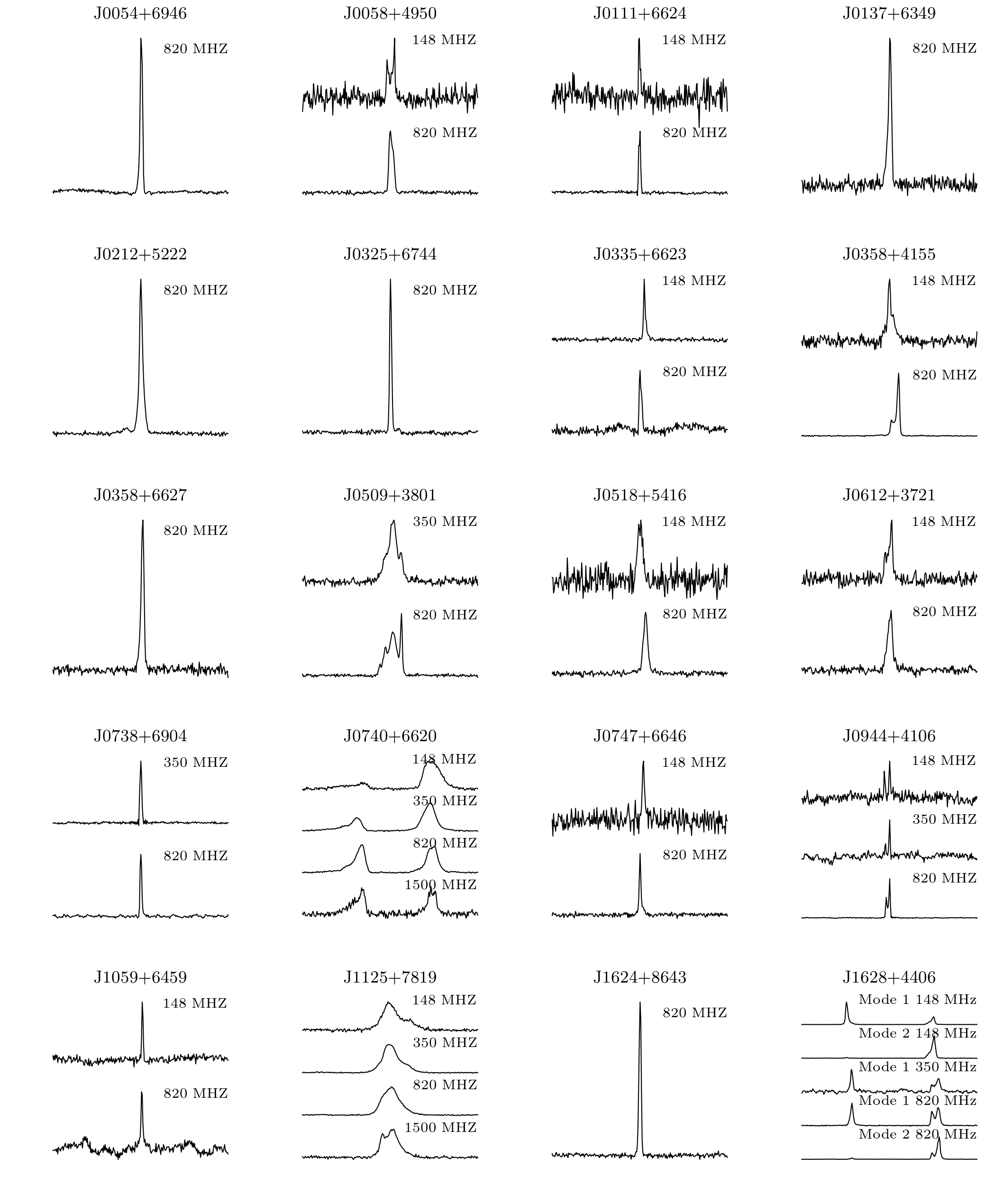
Figure 9: Average pulse profiles for the 45 pulsars presented here. Data from all available observing bands are presented. All profiles have been rotated $180\arcdeg$ from the zero-point pulse phase reference.

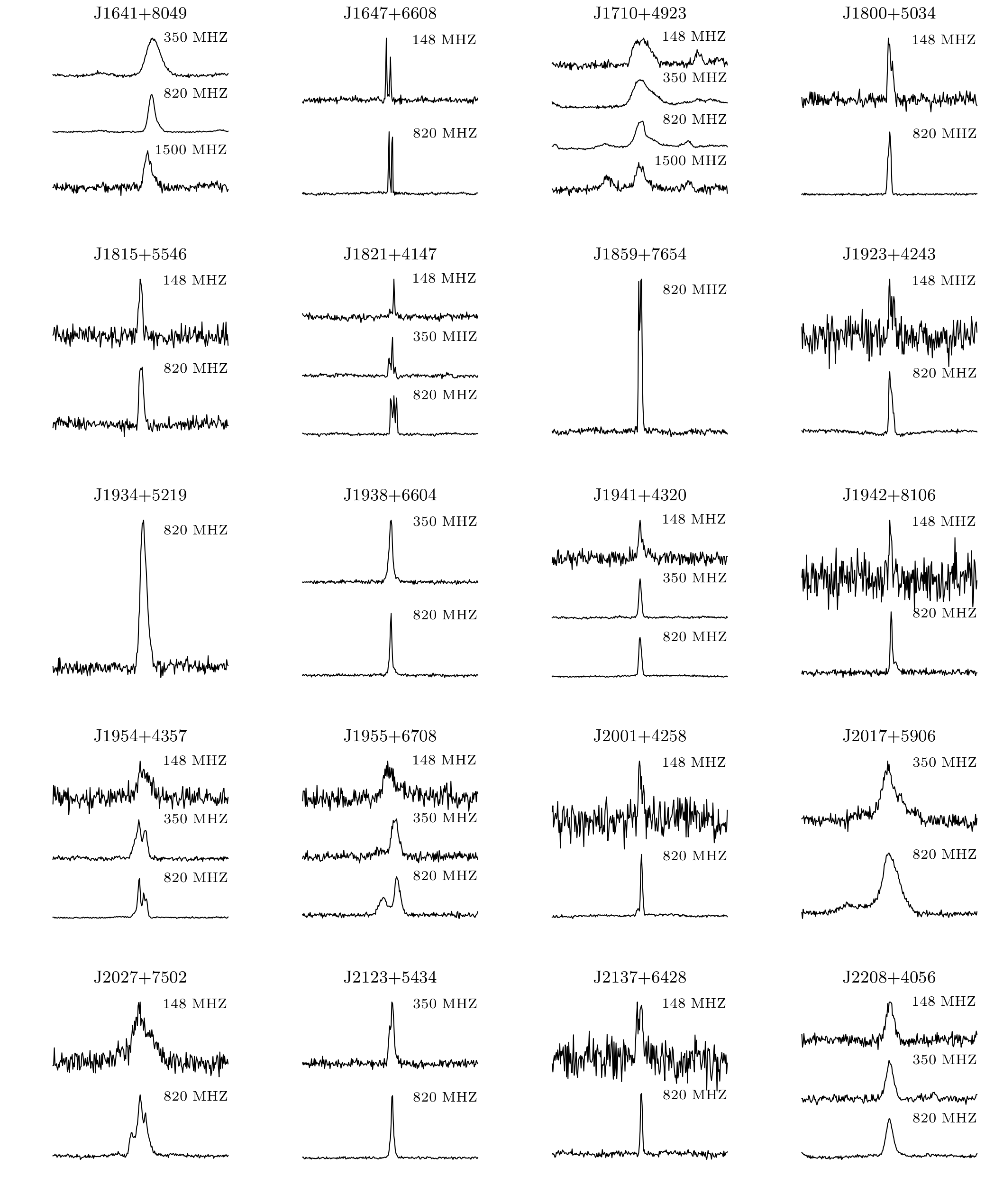
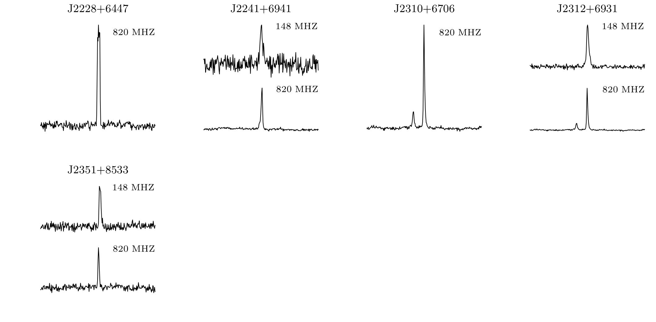
Figure 9: Average pulse profiles for the 45 pulsars presented here. Data from all available observing bands are presented. All profiles have been rotated $180\arcdeg$ from the zero-point pulse phase reference.

The measured rotational parameters and common derived properties of all of our pulsars are shown in Tables 2 and 3, respectively. Table 4 shows positions in a variety of coordinate systems as well as DMs. ELL1 binary timing parameters of four pulsars are shown in Table 5. The locations of all the pulsars presented here on the $P$-$\dot{P}$ diagram are shown in Figure 1. Post-fit timing residuals and integrated pulse profiles are shown in Figures 8 and 9, respectively. In the following sections, we present specific details on pulsars of interest.

5.1 NANOGrav and IPTA Pulsars

One of the primary science goals of the GBNCC survey is finding high-precision MSPs for inclusion in PTAs. The quadrupolar nature of GWs should cause a unique angular correlation between pairs of MSPs in a PTA. Sampling many baselines is essential to firmly establish this quadrupolar signature, and this will be necessary for PTAs to claim a detection of low-frequency GWs. The GBNCC survey is especially well suited to find MSPs at high northern declinations, which have been historically undersampled by sensitive pulsar surveys.

Two MSPs presented here have been included in NANOGrav and the IPTA based on promising early results: PSRs J0740+6620 and J1125+7819. We found it necessary to use the DMX timing model for PSR J1125+7819 to measure epoch-dependent variations in DM. We used a 30-day window for DMX epochs and found typical DM variations of $\sim 10^{-4}$–$10^{-5}\;\mathrm{pc\;cm^{-3}}$, with a maximum $|\Delta\textrm{DM}|=1.7\times 10^{-2}\;\mathrm{pc\;cm^{-3}}$. These results are consistent with DM variations measured in NANOGrav timing (Arzoumanian et al., 2018). PSRs J1710+4923 and J1641+8049 have not been included in PTAs despite relatively low uncertainty on individual TOAs—PSR J1710+4923 because of strong scintillation and PSR J1641+8049 because it is in a black widow binary system.

Table 2: Rotational and Timing Parameters of GBNCC Pulsars

PSR	Name Used In	$\nu$	$\dot{\nu}$	Epoch	Data Span	RMS Residual	$N_{\rm TOA}$	$\chi^{2}_{\rm red}$
	Stovall et al. (2014)	(Hz)	($\textrm{Hz}\;\textrm{s}^{-1}$)	(MJD)	(MJD)	($\mathrm{\mu s}$)
J0054$+$6946	J0053+69	1.200607994501(6)	$-$1.037(1)$\times$10-15	56500.0	56329–56791	542.59	297	0.9
J0058$+$4950	J0059+50	1.00399242379(4)	$-$8.1(2)$\times$10-16	56500.0	56358–56670	1701.9	186	1.9
J0111$+$6624	J0112+66	0.23245693423(2)	$-$4.52(9)$\times$10-16	56500.0	56332–56670	3071.21	131	1.6
J0137$+$6349	J0136+63	1.39282996541(1)	$-$1.862(9)$\times$10-15	56500.0	56329–56670	797.51	276	1.3
J0212$+$5222	J0213+52	2.65684439046(1)	$-$4.6583(9)$\times$10-14	56500.0	56332–56670	376.92	252	1.6
J0325$+$6744	J0325+67	0.732773180015(8)	$-$8.34(5)$\times$10-16	56500.0	56351–56669	952.49	204	2.6
J0335$+$6623	J0338+66	0.56755806947(6)	$-$1.55(3)$\times$10-15	56500.0	56351–56669	1068.56	88	1.2
J0358$+$4155	J0358+42	4.415316459453(4)	$-$2.843(3)$\times$10-15	56500.0	56332–56670	85.32	247	1.1
J0358$+$6627	J0358+66	10.92827132616(2)	$-$1.30(1)$\times$10-15	56500.0	56329–56669	80.73	86	0.9
J0509$+$3801	J0510+38	13.06483380156(2)	$-$1.3538(4)$\times$10-15	56900.0	56336–57474	102.36	791	1.1
J0518$+$5416	J0519+54	2.93942447332(5)	$-$1.448(3)$\times$10-14	56500.0	56336–56669	961.97	207	3.4
J0612$+$3721	J0610+37	2.2529049469(1)	$-$7.6(7)$\times$10-16	56500.0	56336–56669	1373.35	69	1.0
J0738$+$6904	J0737+69	0.14646235983(1)	$-$5.785(8)$\times$10-16	56425.0	56159–56669	2138.93	84	4.0
J0740$+$6620	J0741+66	346.53199660394(1)	$-$1.4658(8)$\times$10-15	56675.0	56156–56908	2.95	383	1.9
J0747$+$6646	J0746+66	2.45278075482(3)	$-$4.08(2)$\times$10-15	56500.0	56336–56669	371.01	73	0.9
J0944$+$4106	J0943+41	0.448544888919(9)	$-$8.894(6)$\times$10-16	56350.0	56046–56669	515.44	165	2.2
J1059$+$6459	J1101+65	0.2753933549(1)	$-$4.35(4)$\times$10-16	56500.0	56478–57215	4371.22	30	0.8
J1125$+$7819	J1122+78	238.00405319610(8)	$-$4.11(5)$\times$10-16	56625.0	56156–57078	11.58	1461	3.8
J1624$+$8643	J1627+86	2.52676461497(1)	$-$1.625(6)$\times$10-15	56500.0	56351–56669	223.5	279	1.1
J1628$+$4406	J1629+43	5.519419001073(2)	$-$5.9032(8)$\times$10-16	56625.0	56017–56973	99.14	2225	3.7
J1641$+$8049	J1649+80	494.76063707093(2)	$-$2.19(2)$\times$10-15	56425.0	56159–56670	5.81	788	2.7
J1647$+$6608	J1647+66	0.62507876955(1)	$-$3.063(6)$\times$10-15	56500.0	56351–56669	690.08	174	1.2
J1710$+$4923	J1710+49	310.536979440897(4)	$-$1.7561(2)$\times$10-15	56850.0	55996–57700	10.76	757	2.3
J1800$+$5034	J1800+50	1.72898175945(3)	$-$3.5(2)$\times$10-16	56500.0	56365–56670	814.31	338	1.2
J1815$+$5546	J1815+55	2.3427772328(2)	$-$5.2(8)$\times$10-16	56500.0	56365–56670	1800.71	103	4.5
J1821$+$4147	J1821+41	0.792482693574(5)	$-$1.0860(6)$\times$10-15	56375.0	56085–56670	625.93	252	1.1
J1859$+$7654	J1859+76	0.71749953039(1)	$-$2.6(8)$\times$10-17	56500.0	56351–56669	682.37	185	1.0
J1923$+$4243	J1921+42	1.68012768584(3)	$-$7.15(1)$\times$10-15	56525.0	56365–56670	520.97	228	1.1
J1934$+$5219	J1935+52	1.75919355395(8)	$-$2.6(4)$\times$10-16	56525.0	56365–56670	2086.41	178	2.3
J1938$+$6604	J1939+66	44.926049244297(5)	$-$3.93(7)$\times$10-17	56550.0	56176–56907	28.02	691	1.4
J1941$+$4320	J1941+43	1.189192897888(8)	$-$1.6224(7)$\times$10-15	56375.0	56081–56670	848.81	286	1.9
J1942$+$8106	J1942+81	4.91259383196(3)	$-$8.9(1)$\times$10-16	56500.0	56332–56670	274.58	115	1.3
J1954$+$4357	J1954+43	0.72095913858(1)	$-$1.145(2)$\times$10-15	56550.0	56081–57015	1485.51	440	1.5
J1955$+$6708	J1953+67	116.74869454326(1)	$-$1.717(6)$\times$10-16	56600.0	56156–57447	48.87	564	3.0
J2001$+$4258	J2001+42	1.390499284334(8)	$-$3.3501(4)$\times$10-14	56500.0	56328–56670	410.55	250	1.1
J2017$+$5906	J2017+59	2.4784478211(1)	$-$1.361(8)$\times$10-15	56575.0	56276–56856	3397.28	321	2.4
J2027$+$7502	J2027+74	1.94092353149(3)	$-$3.35(2)$\times$10-15	56500.0	56351–56669	1371.4	335	1.5
J2123$+$5434	J2122+54	7.20107927874(1)	$-$9.0(5)$\times$10-18	56500.0	56332–57815	92.15	249	1.0
J2137$+$6428	J2137+64	0.57110576181(2)	$-$1.12(1)$\times$10-15	56500.0	56329–56670	1182.98	65	1.1
J2208$+$4056	J2207+40	1.56996372132(3)	$-$1.3022(2)$\times$10-14	56375.0	56081–56670	1882.71	235	1.9
J2228$+$6447	J2229+64	0.52826709593(1)	$-$1.87(8)$\times$10-16	56500.0	56329–56670	1868.72	209	1.1
J2241$+$6941	J2243+69	1.16904199244(2)	$-$3.68(1)$\times$10-15	56500.0	56351–56670	889.58	173	1.4
J2310$+$6706	$\cdots$	0.5141946062(3)	$-$2(1)$\times$10-17	57225.0	57078–57397	1204.93	80	2.5
J2312$+$6931	J2316+69	1.22944554793(3)	$-$9.5(2)$\times$10-16	56500.0	56331–56670	1657.42	146	2.4
J2351$+$8533	J2353+85	0.98840874179(6)	$-$8.6(3)$\times$10-16	56500.0	56332–56669	1398.72	42	1.1

Note. — Where aplicable, we give the pulsar name used when presenting discovery parameters in Stovall et al. (2014). All timing models use the DE430 Solar system ephemeris and are referenced to the TT(BIPM) time standard. Values in parentheses are the $1$-$\sigma$ uncertainty in the last digit as reported by TEMPO.

Table 3: Derived Common Properties of GBNCC Pulsars

PSR	$P$	$\dot{P}$	$\tau_{\rm c}$	$B_{\rm surf}$	$\dot{E}_{\rm rot}$	$D^{\rm NE2001}_{\rm DM}$	$D^{\rm YMW16}_{\rm DM}$
	(s)	($\textrm{s}\;\textrm{s}^{-1}$)	(yr)	(G)	($\textrm{erg}\;\textrm{s}^{-1}$)	(kpc)	(kpc)
J0054$+$6946	0.832911328744(4)	7.194(8)$\times$10-16	1.834(2)$\times$107	7.832(4)$\times$1011	4.915(5)$\times$1031	4.3	2.8
J0058$+$4950	0.99602345227(4)	8.0(2)$\times$10-16	1.97(5)$\times$107	9.0(1)$\times$1011	3.20(7)$\times$1031	2.8	2.6
J0111$+$6624	4.3018721007(3)	8.4(2)$\times$10-15	8.1(2)$\times$106	6.07(6)$\times$1012	4.15(9)$\times$1030	3.4	2.4
J0137$+$6349	0.717962726847(7)	9.60(5)$\times$10-16	1.185(6)$\times$107	8.40(2)$\times$1011	1.024(5)$\times$1032	44.3	9.1
J0212$+$5222	0.376386364060(2)	6.599(1)$\times$10-15	9.037(2)$\times$105	1.5946(1)$\times$1012	4.8860(9)$\times$1033	1.5	1.6
J0325$+$6744	1.36467876728(1)	1.553(9)$\times$10-15	1.393(8)$\times$107	1.473(4)$\times$1012	2.41(1)$\times$1031	2.3	1.9
J0335$+$6623	1.7619342474(2)	4.81(9)$\times$10-15	5.8(1)$\times$106	2.95(3)$\times$1012	3.47(7)$\times$1031	2.3	1.9
J0358$+$4155	0.2264843322519(2)	1.458(1)$\times$10-16	2.461(2)$\times$107	1.8388(9)$\times$1011	4.956(5)$\times$1032	1.6	1.5
J0358$+$6627	0.0915057807547(2)	1.09(1)$\times$10-17	1.33(1)$\times$108	3.20(2)$\times$1010	5.62(5)$\times$1032	2.2	1.9
J0509$+$3801	0.0765413487220(1)	7.931(2)$\times$10-18	1.5291(5)$\times$108	2.4929(4)$\times$1010	6.982(2)$\times$1032	1.9	1.6
J0518$+$5416	0.340202651599(6)	1.676(3)$\times$10-15	3.217(6)$\times$106	7.639(7)$\times$1011	1.680(3)$\times$1033	1.5	1.4
J0612$+$3721	0.44387136767(2)	1.5(1)$\times$10-16	4.7(4)$\times$107	2.6(1)$\times$1011	6.8(6)$\times$1031	1.2	1.1
J0738$+$6904	6.8276928023(5)	2.697(4)$\times$10-14	4.012(6)$\times$106	1.373(1)$\times$1013	3.345(5)$\times$1030	0.8	1.1
J0740$+$6620	0.0028857364104907(1)	1.2206(7)$\times$10-20	3.746(2)$\times$109	1.8990(5)$\times$108	2.005(1)$\times$1034	0.7	0.9
J0747$+$6646	0.407700524409(4)	6.78(3)$\times$10-16	9.53(4)$\times$106	5.32(1)$\times$1011	3.95(2)$\times$1032	1.2	1.9
J0944$+$4106	2.22943126698(4)	4.421(3)$\times$10-15	7.990(6)$\times$106	3.176(1)$\times$1012	1.575(1)$\times$1031	0.8	2.7
J1059$+$6459	3.631169678(2)	5.73(5)$\times$10-15	1.003(9)$\times$107	4.62(2)$\times$1012	4.73(4)$\times$1030	0.8	1.9
J1125$+$7819	0.004201609117875(1)	7.26(8)$\times$10-21	9.2(1)$\times$109	1.77(1)$\times$108	3.87(4)$\times$1033	0.6	0.8
J1624$+$8643	0.395763022038(2)	2.55(1)$\times$10-16	2.46(1)$\times$107	3.211(6)$\times$1011	1.621(6)$\times$1032	3.0	0.5
J1628$+$4406	0.18117848994714(5)	1.9378(3)$\times$10-17	1.4814(2)$\times$108	5.9952(4)$\times$1010	1.2863(2)$\times$1032	0.6	8.8
J1641$+$8049	0.0020211793846822(1)	8.95(7)$\times$10-21	3.58(3)$\times$109	1.361(5)$\times$108	4.28(3)$\times$1034	1.7	2.1
J1647$+$6608	1.59979837535(3)	7.84(2)$\times$10-15	3.233(7)$\times$106	3.583(4)$\times$1012	7.56(2)$\times$1031	1.3	3.0
J1710$+$4923	0.00322022839856445(4)	1.8211(2)$\times$10-20	2.8017(3)$\times$109	2.4502(1)$\times$108	2.1530(2)$\times$1034	0.7	0.5
J1800$+$5034	0.57837510115(1)	1.19(5)$\times$10-16	7.7(4)$\times$107	2.65(6)$\times$1011	2.4(1)$\times$1031	1.4	1.9
J1815$+$5546	0.42684382706(4)	9(2)$\times$10-17	7(1)$\times$107	2.0(2)$\times$1011	4.8(8)$\times$1031	50.0	25.0
J1821$+$4147	1.261857209133(9)	1.7292(9)$\times$10-15	1.1562(6)$\times$107	1.4946(4)$\times$1012	3.398(2)$\times$1031	2.5	4.4
J1859$+$7654	1.39372913521(2)	5(2)$\times$10-17	4(1)$\times$108	2.7(4)$\times$1011	6(2)$\times$1029	2.9	6.0
J1923$+$4243	0.59519285851(1)	2.534(5)$\times$10-15	3.721(8)$\times$106	1.243(1)$\times$1012	4.75(1)$\times$1032	3.2	4.7
J1934$+$5219	0.56844228297(3)	8(1)$\times$10-17	1.1(2)$\times$108	2.2(2)$\times$1011	1.8(3)$\times$1031	4.5	7.7
J1938$+$6604	0.022258801226038(2)	1.95(3)$\times$10-20	1.81(3)$\times$1010	6.66(6)$\times$108	7.0(1)$\times$1031	2.3	3.4
J1941$+$4320	0.840906468392(6)	1.1472(5)$\times$10-15	1.1614(5)$\times$107	9.938(2)$\times$1011	7.617(3)$\times$1031	4.4	6.5
J1942$+$8106	0.203558452868(1)	3.68(6)$\times$10-17	8.8(1)$\times$107	8.76(7)$\times$1010	1.72(3)$\times$1032	2.1	3.5
J1954$+$4357	1.38704116015(2)	2.202(3)$\times$10-15	9.98(1)$\times$106	1.768(1)$\times$1012	3.258(4)$\times$1031	7.1	5.3
J1955$+$6708	0.0085654062678141(8)	1.259(4)$\times$10-20	1.078(4)$\times$1010	3.323(6)$\times$108	7.91(3)$\times$1032	3.4	10.1
J2001$+$4258	0.719166137852(4)	1.7327(2)$\times$10-14	6.5762(8)$\times$105	3.5717(2)$\times$1012	1.8390(2)$\times$1033	3.3	3.8
J2017$+$5906	0.40347833490(2)	2.22(1)$\times$10-16	2.88(2)$\times$107	3.026(9)$\times$1011	1.332(8)$\times$1032	3.3	3.9
J2027$+$7502	0.515218649152(8)	8.90(5)$\times$10-16	9.17(5)$\times$106	6.85(2)$\times$1011	2.57(1)$\times$1032	1.0	0.8
J2123$+$5434	0.1388680725891(2)	1.7(1)$\times$10-19	1.27(7)$\times$1010	5.0(1)$\times$109	2.6(1)$\times$1030	2.1	1.8
J2137$+$6428	1.75098916326(7)	3.43(4)$\times$10-15	8.1(1)$\times$106	2.48(1)$\times$1012	2.53(3)$\times$1031	4.8	3.8
J2208$+$4056	0.63695739361(1)	5.283(1)$\times$10-15	1.9102(4)$\times$106	1.8561(2)$\times$1012	8.071(2)$\times$1032	1.0	0.8
J2228$+$6447	1.89298180355(5)	6.7(3)$\times$10-16	4.5(2)$\times$107	1.14(3)$\times$1012	3.9(2)$\times$1030	46.9	6.9
J2241$+$6941	0.85540126571(1)	2.693(8)$\times$10-15	5.03(1)$\times$106	1.536(2)$\times$1012	1.699(5)$\times$1032	2.9	2.5
J2310$+$6706	1.944788973(1)	6(5)$\times$10-17	5(4)$\times$108	3(1)$\times$1011	2(3)$\times$1029	3.5	2.7
J2312$+$6931	0.81337477832(2)	6.3(1)$\times$10-16	2.04(4)$\times$107	7.25(6)$\times$1011	4.63(8)$\times$1031	2.8	2.4
J2351$+$8533	1.01172719111(6)	8.8(3)$\times$10-16	1.83(7)$\times$107	9.5(2)$\times$1011	3.3(1)$\times$1031	1.9	2.6

Note. — $D_{\rm DM}$ is calculated using the NE2001 Cordes & Lazio (2002) or YMW16 (Yao et al., 2017) Galactic free electron density models, as indicated. A fractional uncertainty of 50% is not uncommon. Derived parameters have not been corrected for the Shklovskii effect. $\dot{E}$ is calculated assuming a moment of inertia $I=10^{45}\;\textrm{gm}\,\textrm{cm}^{2}$. Values in parentheses are the $1$-$\sigma$ uncertainty in the last digit, calculated by propogating uncertainties in measured parameters reported by TEMPO.

Table 4: Coordinates and DMs of GBNCC Pulsars

PSR	Measured			Derived
	$\lambda$ ($\arcdeg$)	$\beta$ ($\arcdeg$)	DM ($\mathrm{pc\;cm^{-3}}$)	$\alpha$ (J2000)	$\delta$ (J2000)	$\ell$ ($\arcdeg$)	$b$ ($\arcdeg$)
J0054$+$6946	53.17957(2)	55.915268(8)	116.52(5)	$00^{\rm h}\,54^{\rm m}\,59\,\fs 109$	$69\arcdeg\,46\arcmin\,16\,\farcs 9$	123.24077	6.90173
J0058$+$4950	35.9410(1)	39.55191(6)	66.953(7)	$00^{\rm h}\,58^{\rm m}\,09\,\fs 989$	$49\arcdeg\,50\arcmin\,26\,\farcs 0$	124.04528	-13.01663
J0111$+$6624	51.3828(4)	52.3710(1)	111.20(3)	$01^{\rm h}\,11^{\rm m}\,21\,\fs 862$	$66\arcdeg\,24\arcmin\,10\,\farcs 9$	124.92791	3.60854
J0137$+$6349	52.48260(5)	48.69309(3)	285.50(6)	$01^{\rm h}\,37^{\rm m}\,13\,\fs 362$	$63\arcdeg\,49\arcmin\,34\,\farcs 4$	127.95520	1.40191
J0212$+$5222	50.60763(2)	36.42041(1)	38.21(3)	$02^{\rm h}\,12^{\rm m}\,52\,\fs 136$	$52\arcdeg\,22\arcmin\,49\,\farcs 5$	135.33111	-8.51996
J0325$+$6744	69.66385(5)	47.02620(3)	65.28(5)	$03^{\rm h}\,25^{\rm m}\,05\,\fs 117$	$67\arcdeg\,44\arcmin\,59\,\farcs 4$	136.71527	9.08929
J0335$+$6623	70.4110(3)	45.3827(3)	66.726(2)	$03^{\rm h}\,35^{\rm m}\,57\,\fs 077$	$66\arcdeg\,23\arcmin\,23\,\farcs 6$	138.38339	8.58769
J0358$+$4155	66.154390(4)	20.973526(6)	46.325(1)	$03^{\rm h}\,58^{\rm m}\,03\,\fs 174$	$41\arcdeg\,55\arcmin\,19\,\farcs 1$	156.11209	-8.62040
J0358$+$6627	73.496599(8)	44.753531(6)	62.33(1)	$03^{\rm h}\,58^{\rm m}\,37\,\fs 926$	$66\arcdeg\,27\arcmin\,46\,\farcs 6$	140.12843	10.06385
J0509$+$3801	79.7362277(8)	15.030898(4)	69.0794(9)	$05^{\rm h}\,09^{\rm m}\,31\,\fs 788$	$38\arcdeg\,01\arcmin\,18\,\farcs 1$	168.27474	-1.18699
J0518$+$5416	83.01300(5)	31.09029(8)	42.330(5)	$05^{\rm h}\,18^{\rm m}\,53\,\fs 198$	$54\arcdeg\,16\arcmin\,50\,\farcs 0$	155.91644	9.55747
J0612$+$3721	92.6070(1)	13.9507(6)	39.270(6)	$06^{\rm h}\,12^{\rm m}\,44\,\fs 087$	$37\arcdeg\,21\arcmin\,40\,\farcs 2$	175.44220	9.08013
J0738$+$6904	102.51871(7)	46.69934(9)	17.22(2)	$07^{\rm h}\,38^{\rm m}\,022\,\fs 61$	$69\arcdeg\,04\arcmin\,20\,\farcs 1$	146.59345	29.37720
J0740$+$6620	103.7591384(1)	44.1025059(1)	14.92(2)	$07^{\rm h}\,40^{\rm m}\,45\,\fs 799$	$66\arcdeg\,20\arcmin\,33\,\farcs 6$	149.72969	29.59937
J0747$+$6646	104.53950(2)	44.69663(5)	27.576(3)	$07^{\rm h}\,47^{\rm m}\,39\,\fs 689$	$66\arcdeg\,46\arcmin\,56\,\farcs 8$	149.21764	30.28271
J0944$+$4106	134.006413(9)	25.83992(3)	21.41(3)	$09^{\rm h}\,44^{\rm m}\,18\,\fs 141$	$41\arcdeg\,06\arcmin\,04\,\farcs 6$	180.43732	49.37512
J1059$+$6459	131.4687(7)	51.9583(6)	18.5(4)	$10^{\rm h}\,59^{\rm m}\,27\,\fs 511$	$64\arcdeg\,59\arcmin\,31\,\farcs 8$	140.25104	48.19754
J1125$+$7819	115.6292886(9)	62.4520225(4)	11.219201	$11^{\rm h}\,25^{\rm m}\,59\,\fs 851$	$78\arcdeg\,19\arcmin\,48\,\farcs 7$	128.28875	37.89467
J1624$+$8643	93.79282(3)	69.51940(1)	46.43(2)	$16^{\rm h}\,24^{\rm m}\,032\,\fs 75$	$86\arcdeg\,43\arcmin\,13\,\farcs 2$	119.92489	29.05717
J1628$+$4406	229.913199(1)	64.4120718(2)	7.32981(2)	$16^{\rm h}\,28^{\rm m}\,50\,\fs 313$	$44\arcdeg\,06\arcmin\,42\,\farcs 6$	69.23851	43.61575
J1641$+$8049	101.8728674(9)	74.8941763(2)	31.08960(3)	$16^{\rm h}\,41^{\rm m}\,20\,\fs 843$	$80\arcdeg\,49\arcmin\,52\,\farcs 9$	113.84003	31.76257
J1647$+$6608	174.9821(4)	82.74687(3)	22.55(7)	$16^{\rm h}\,47^{\rm m}\,32\,\fs 522$	$66\arcdeg\,08\arcmin\,22\,\farcs 2$	97.18025	37.03415
J1710$+$4923	243.4177674(2)	71.67561410(7)	7.08493(2)	$17^{\rm h}\,10^{\rm m}\,04\,\fs 442$	$49\arcdeg\,23\arcmin\,11\,\farcs 4$	75.92934	36.44891
J1800$+$5034	270.4263(1)	74.01172(4)	22.71(6)	$18^{\rm h}\,00^{\rm m}\,44\,\fs 372$	$50\arcdeg\,34\arcmin\,21\,\farcs 7$	78.12962	28.43981
J1815$+$5546	281.2542(7)	79.0649(2)	58.999(7)	$18^{\rm h}\,15^{\rm m}\,05\,\fs 739$	$55\arcdeg\,46\arcmin\,23\,\farcs 2$	84.31588	27.13337
J1821$+$4147	279.69363(3)	65.03943(1)	40.673(3)	$18^{\rm h}\,21^{\rm m}\,52\,\fs 346$	$41\arcdeg\,47\arcmin\,02\,\farcs 5$	69.53713	22.90515
J1859$+$7654	72.6850(2)	78.72083(4)	47.25(7)	$18^{\rm h}\,59^{\rm m}\,36\,\fs 019$	$76\arcdeg\,54\arcmin\,55\,\farcs 6$	108.36384	25.91076
J1923$+$4243	305.93303(4)	63.58758(4)	52.99(5)	$19^{\rm h}\,23^{\rm m}\,015\,\fs 24$	$42\arcdeg\,43\arcmin\,18\,\farcs 6$	74.71528	12.64331
J1934$+$5219	320.8887(1)	71.6218(1)	71.9(1)	$19^{\rm h}\,34^{\rm m}\,23\,\fs 892$	$52\arcdeg\,19\arcmin\,57\,\farcs 4$	84.49263	15.04604
J1938$+$6604	8.602915(1)	80.1174609(2)	41.2427(1)	$19^{\rm h}\,38^{\rm m}\,56\,\fs 919$	$66\arcdeg\,04\arcmin\,31\,\farcs 7$	97.94564	20.03050
J1941$+$4320	313.54787(3)	62.971984(8)	79.361(8)	$19^{\rm h}\,41^{\rm m}\,58\,\fs 915$	$43\arcdeg\,20\arcmin\,06\,\farcs 3$	76.84556	9.86437
J1942$+$8106	75.79591(5)	74.12426(1)	40.24(3)	$19^{\rm h}\,42^{\rm m}\,54\,\fs 669$	$81\arcdeg\,06\arcmin\,17\,\farcs 3$	113.37123	24.82517
J1954$+$4357	318.69172(4)	62.63881(2)	130.30(5)	$19^{\rm h}\,54^{\rm m}\,038\,\fs 45$	$43\arcdeg\,57\arcmin\,37\,\farcs 3$	78.52732	8.16863
J1955$+$6708	16.178385(1)	78.7214729(2)	57.1478(1)	$19^{\rm h}\,55^{\rm m}\,38\,\fs 764$	$67\arcdeg\,08\arcmin\,15\,\farcs 1$	99.68213	18.93834
J2001$+$4258	320.10684(2)	61.24332(2)	54.93(3)	$20^{\rm h}\,01^{\rm m}\,010\,\fs 59$	$42\arcdeg\,58\arcmin\,06\,\farcs 2$	78.27728	6.64261
J2017$+$5906	350.7866(2)	72.89756(3)	60.28(6)	$20^{\rm h}\,17^{\rm m}\,44\,\fs 555$	$59\arcdeg\,06\arcmin\,46\,\farcs 9$	93.60825	12.90340
J2027$+$7502	51.5269(2)	75.59357(2)	11.71(1)	$20^{\rm h}\,27^{\rm m}\,23\,\fs 274$	$75\arcdeg\,02\arcmin\,29\,\farcs 2$	108.36769	20.31252
J2123$+$5434	358.500835(3)	63.277719(2)	31.760(3)	$21^{\rm h}\,23^{\rm m}\,21\,\fs 681$	$54\arcdeg\,34\arcmin\,07\,\farcs 7$	95.69847	3.09706
J2137$+$6428	20.1556(4)	68.10698(6)	106.0(3)	$21^{\rm h}\,37^{\rm m}\,20\,\fs 257$	$64\arcdeg\,28\arcmin\,41\,\farcs 7$	103.85139	9.06360
J2208$+$4056	354.46060(4)	47.91605(4)	11.837(9)	$22^{\rm h}\,08^{\rm m}\,01\,\fs 991$	$40\arcdeg\,56\arcmin\,01\,\farcs 8$	92.57410	-12.11198
J2228$+$6447	27.9436(2)	63.61524(4)	193.6(2)	$22^{\rm h}\,28^{\rm m}\,40\,\fs 502$	$64\arcdeg\,47\arcmin\,19\,\farcs 4$	108.46152	6.00724
J2241$+$6941	39.1473(1)	65.08555(2)	67.67(7)	$22^{\rm h}\,41^{\rm m}\,20\,\fs 295$	$69\arcdeg\,41\arcmin\,59\,\farcs 7$	112.02560	9.63205
J2310$+$6706	37.3837(3)	61.4356(4)	97.7(2)	$23^{\rm h}\,10^{\rm m}\,42\,\fs 077$	$67\arcdeg\,06\arcmin\,52\,\farcs 1$	113.35114	6.13557
J2312$+$6931	41.8523(2)	62.62711(4)	71.6(1)	$23^{\rm h}\,12^{\rm m}\,038\,\fs 93$	$69\arcdeg\,31\arcmin\,04\,\farcs 0$	114.43546	8.29219
J2351$+$8533	78.8764(3)	66.3376(2)	38.5(4)	$23^{\rm h}\,51^{\rm m}\,03\,\fs 261$	$85\arcdeg\,33\arcmin\,20\,\farcs 7$	121.67724	22.83186

Note. — Ecliptic coordinates use the IERS2010 value of the obliquity of the ecliptic referenced to J2000 (Capitaine et al., 2003). Values in parentheses are the $1$-$\sigma$ uncertainty in the last digit as reported by TEMPO.

Table 5: ELL1 Binary Parameters of GBNCC Pulsars

Parameter	J0740$+$6620	J1125$+$7819	J1641$+$8049	J1938$+$6604
Measured Parameters
$P_{\rm B}$ (d)	4.766944616(3)	15.35544590(2)	0.0908739634(1)	2.467162727(1)
$a\sin{i}/c$ (s)	3.977556(1)	12.1924288(7)	0.0640793(3)	8.950738(1)
$T_{\rm asc}$ (MJD)	56155.3684710(2)	56157.4763453(3)	56220.5100737(1)	56366.0967005(1)
$\epsilon_{1}$	$-$5.6(4)$\times$10-6	$-$1.28(1)$\times$10-5	0.000111(8)	4.8(3)$\times$10-6
$\epsilon_{2}$	$-$2.0(2)$\times$10-6	1.0(1)$\times$10-6	$-$5.4(6)$\times$10-5	$-$2.81(3)$\times$10-5
Derived Parameters
$T_{0}$ (MJD)	56156.30(3)	56153.82(2)	56220.4939(8)	56366.030(5)
$e$	5.9(4)$\times$10-6	1.29(1)$\times$10-5	0.000123(8)	2.85(3)$\times$10-5
$\omega$ ($\arcdeg$)	1.23(4)	$-$1.495(8)	$-$1.12(5)	$-$0.17(1)
$f_{\rm M}$ ($\mathrm{M_{\sun}}$)	0.002973387(3)	0.008253317(1)	3.42102(5)$\times$10-5	0.12649217(6)
$M_{\rm c,min}$ ($\mathrm{M_{\sun}}$)	0.2	0.29	0.04	0.87

Note. — All timing models presented here use the ELL1 binary model, which is appropriate for low-eccentricity orbits. Binary parameters for the relativistic binary PSR J0509+3801 are shown in Table 7. Values in parentheses are the $1$-$\sigma$ uncertainty in the last digit as reported by TEMPO.

Table 6: Proper Motions and Kinematic Corrections for Five GBNCC Pulsars

PSR	$\mu_{\lambda}$	$\mu_{\beta}$	$D_{\rm DM}$	$v_{\rm t}$	$\dot{P}_{\rm G}$	$\dot{P}_{\rm S}$	$B_{\rm surf}$	$\tau_{\rm c}$	$\dot{E}$
	($\mathrm{mas}\,\textrm{yr}^{-1}$)	($\mathrm{mas}\,\textrm{yr}^{-1}$)	(kpc)	($\textrm{km}\,\textrm{s}^{-1}$)	($10^{-21}$)	($10^{-21}$)	($10^{8}\;\textrm{G}$)	(Gyr)	($10^{33}\;\textrm{erg}\,\textrm{s}^{-1}$)
J0740+6620	$-3.2(4)$	$-33.7(6)$	0.7	112	$-0.14$	5.6	1.4	6.8	11
			0.9	144	$-0.13$	7.2	1.2	8.9	8.4
J1125+7819	$-$$20(3)$	$-$$25(3)$	0.6	91	-0.40	6.3	0.77	48	0.73
			0.8	121	-0.44	8.4	$\cdots$	$\cdots$	$\cdots$
J1641+8049	$-11(1)$	$-$$37(3)$	1.7	311	-0.32	12	$\cdots$	$\cdots$	$\cdots$
			2.1	384	-0.35	15	$\cdots$	$\cdots$	$\cdots$
J1710+4923	$-50.4(2)$	$-44.7(2)$	0.7	224	-0.41	25	$\cdots$	$\cdots$	$\cdots$
			0.5	160	-0.34	18	0.43	92	0.65
J1955+6708	$-3(1)$	$-$$10(2)$	3.4	168	-2.2	2.9	3.2	11	0.75
			10.1	500	-2.9	8.6	2.5	20	0.43

Note. — Values of $B_{\rm surf}$, $\tau_{\rm c}$, and $\dot{E}$ that have been corrected for the Shklovskii effect are shown for pulsars where $\dot{P}_{\rm S}<\dot{P}_{\rm obs}$.

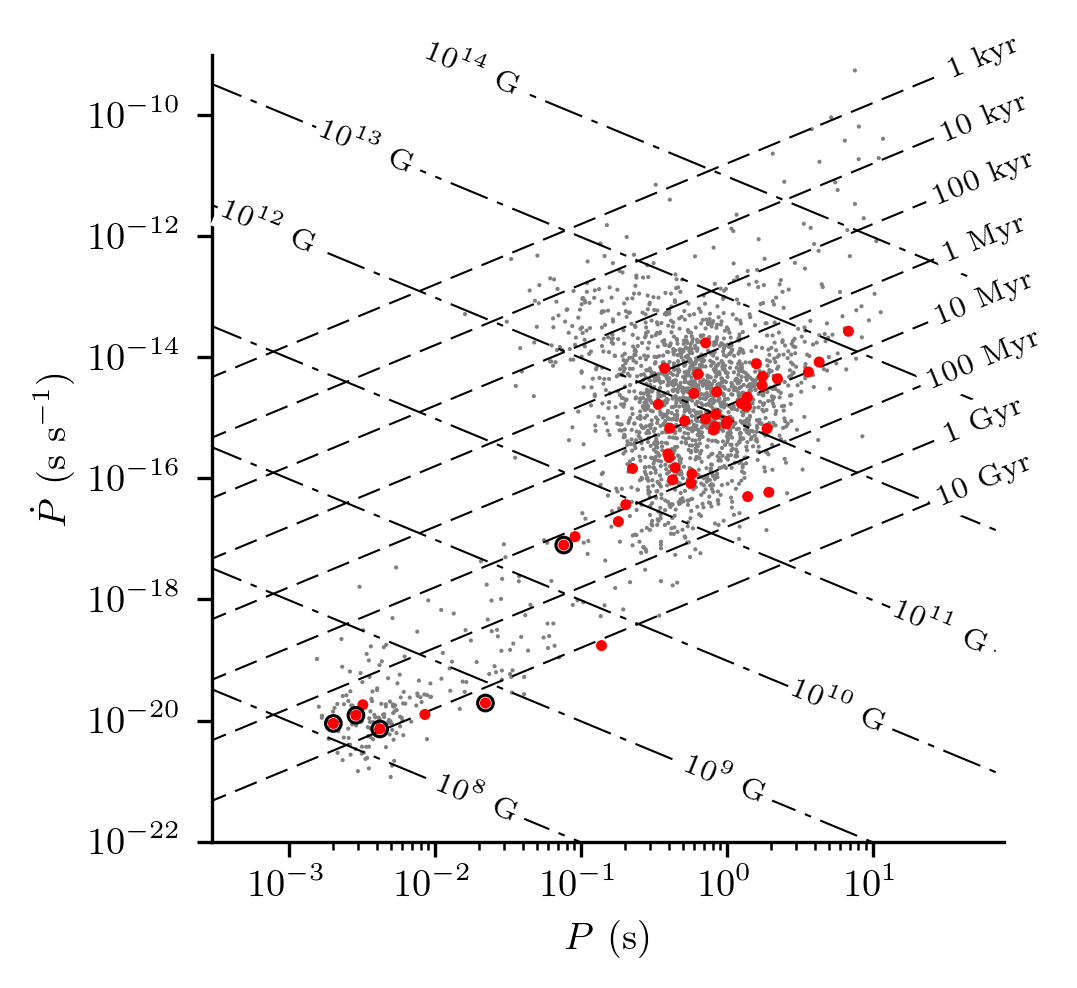
Figure 1: Spin period vs period derivative for the 45 pulsars presented here (red circles) as well as all the pulsars listed in the ATNF pulsar catalog^a (gray points; Manchester et al. 2005). Binary pulsars are indicated with a black circle. Dashed lines show constant characteristic age and dot-dashed lines show constant surface magnetic field.

^ahttp://www.atnf.csiro.au/research/pulsar/psrcat

5.2 Proper Motions and Kinematic Corrections

We have measured timing proper motions for five MSPs: PSRs J0740+6620, J1125+7819, J1641+8049, J1710+4923, and J1955+6708. Table 6 lists the measured proper motions, estimated transverse velocity, $v_{\rm t}$ calculated using the DM-inferred distances in both the NE2001 Cordes & Lazio (2002) and YMW16 (Yao et al., 2017) models, and kinematic corrections.

The observed pulsar spin down is a contribution of several effects:

$$\dot{P}_{\rm obs}=\dot{P}_{\rm int}+\dot{P}_{\rm G}+\dot{P}_{\rm S}$$ (4)

where $\dot{P}_{\rm G}$ is caused by acceleration between the pulsar and Solar System Barycenter in a differential Galactic potential and $\dot{P}_{\rm s}$ is the Shklovskii effect for pulsars. Following Nice & Taylor (1995), the bias arising from acceleration perpdendicular to the Galactic plane ($a_{z}$) is given by

$$\frac{\dot{P}_{\rm G,\perp}}{P}=\frac{a_{z}\sin{b}}{c}$$ (5)

where $b$ is the Galactic latitude and $a_{z}$ is

$$\frac{a_{z}}{c}=-1.09\times 10^{-19}\textrm{s}^{-1}\left[\frac{1.25z}{(z^{2}+0.0324)^{1/2}}+0.58z\right],$$ (6)

where $z=(D/\textrm{kpc})\,\sin{b}$. The planar component is given by

$$\frac{\dot{P}_{\rm G,p}}{P}=-\cos{b}\left(\frac{\Theta_{0}^{2}}{c\,R_{0}}\right)\left(\cos{\ell}+\frac{\beta}{\sin^{2}{\ell}+\beta^{2}}\right)$$ (7)

where $\Theta_{0}=240\;\textrm{km}\,\textrm{s}^{-1}$ is the Sun’s galactocentric velocity, $R_{0}=8.34\;\textrm{kpc}$ is the Sun’s galactocentric distance, and $\beta=(D_{\rm DM}/R_{0})\;\cos{b}-\cos{\ell}$, and $\ell$ is the Galactic longitude. The Shklovskii effect (Shklovskii, 1970) is

$$\frac{\dot{P}_{\rm S}}{P}=2.43\times 10^{-21}\;\textrm{s}^{-1}\left(\frac{D_{\rm DM}}{\textrm{kpc}}\right)\left(\frac{\mu}{10^{-3}\;\arcsec\;\textrm{yr}^{-1}}\right)^{2},$$ (8)

Note that in the case of PSRs J1125+7819, J1641+8049, and J1710+4923, the DM-inferred distance under one or both of the NE2001 and YMW16 models leads to values of $\dot{P}_{\rm S}$ larger than the observed $\dot{P}$. None of these pulsars show any evidence that they are being spun up via accretion, so in all three cases $\dot{P}_{\rm int}$ should be positive. Since $|\dot{P}_{\rm G}|\ll\dot{P}_{\rm S}$ in these cases, we can ignore the Galactic acceleration component and enforce $\dot{P}_{\rm S}<\dot{P}_{\rm obs}$ thereby setting an upper limit on the distances (note that we do not use these distance limits to re-estimate $\dot{P}_{\rm G}$). For PSR J1125+7819, $D<0.7\;\textrm{kpc}$ and $v_{\rm t}<104\;\textrm{km}\,\textrm{s}^{-1}$; PSR J1641+8049, $D<1.2\;\textrm{kpc}$ and $v_{\rm t}<230\;\textrm{km}\,\textrm{s}^{-1}$; for PSR J1710+4923, $D<0.5\;\textrm{kpc}$ and $v_{\rm t}<160\;\textrm{km},\textrm{s}^{-1}$.

The mean transverse velocity of our sample of MSPs is $\mu_{v}=152\;\textrm{km}\,\textrm{s}^{-1}$, with a standard deviation of $\sigma_{v}=48\;\textrm{km}\,\textrm{s}^{-1}$ using the NE2001 DM-inferred distances, and $\mu_{v}=234\;\textrm{km}\,\textrm{s}^{-1}$, $\sigma_{v}=143\;\textrm{km}\,\textrm{s}^{-1}$ using the YMW16 DM-inferred distances (here we use the upper limits on $v_{\rm t}$ as appropriate). Uncertainty in the DM-inferred distances makes a precise measurement of transverse velocity difficult. With this caveat in mind, the velocities that we estimate are somewhat higher than those found by other authors, though still within one to two standard deviations: Toscano et al. (1999) find $\mu_{v}=85\;\textrm{km}\,\textrm{s}^{-1},\sigma_{v}=13\;\textrm{km}\,\textrm{s}^{-1}$ for a sample of 13 MSPs; Hobbs et al. (2005) find $\mu_{v}=87\;\textrm{km}\,\textrm{s}^{-1},\sigma_{v}=13\;\textrm{km}\,\textrm{s}^{-1}$ for a sample of 35 MSPs; and Gonzalez et al. (2011) find $\mu_{v}=88\;\textrm{km}\,\textrm{s}^{-1},\sigma_{v}=12\;\textrm{km}\,\textrm{s}^{-1}$ for a sample of five MSPs.

Table 7: Binary Parameters of PSR J0509+3801

Parameter	Value
Measured Parameters
$P_{\rm b}$ (d) xxxxxxxxxxxxxxxxxxxxxx	0.379583785(3)
$a\sin{i}/c$ (s)	2.0506(3)
$T_{0}$ (MJD)	56075.412714(3)
$e$	0.586400(6)
$\omega$ ($\arcdeg$)	127.77(1)
$M_{\rm tot}$ ($\mathrm{M_{\sun}}$)	2.805(3)
$M_{\rm c}$ ($\mathrm{M_{\sun}}$)	1.46(8)
Derived Parameters
$M_{\rm p}$ ($\mathrm{M_{\sun}}$)	1.34(8)
$f_{\rm M}$ ($\mathrm{M_{\sun}}$)	0.06425(3)
$\dot{\omega}$ ($\arcdeg\;\textrm{yr}^{-1}$)	3.031
$\gamma$ (s)	0.0046
$\dot{P}_{\rm b}$ ($10^{-12}$)	$-1.39$
$\sin{i}$	0.55

Note. — Values in parentheses are the $1$-$\sigma$ uncertainty in the last digit as reported by TEMPO.

5.3 Discussions of Individual Systems

5.3.1 PSR J0509+3801: A New Double Neutron Star System

Figure 2: Estimates of the posterior probability density and marginalized distribution functions (blue-solid curves) for mass estimates of the PSR J0509+3801 system. The regions of allowed masses for individual PK parameters are shown as color-shaded curves in the density map; the thickness of each color-shaded curve represents the 1$\sigma$ uncertainty determined by TEMPO (note that the uncertainties on $\dot{\omega}$ are too small to be visible on this scale). The red-solid lines are the median values for each component mass, and the red-dashed lines represent the edges of the 68.3% credible intervals.

PSR J0509+3801 is part of a highly eccentric binary system with $P_{\rm b}=9.11\;\textrm{hr}$ and $e=0.586$. Early in our timing campaign we measured a significant change in the longitude of periastron, $\dot{\omega}=3.031(2)\arcdeg\;\textrm{yr}^{-1}$. In general relativity (GR), $\dot{\omega}$ is related to the total system mass and our measured value implies $M_{\rm tot}=2.81\;\mathrm{M_{\sun}}$. Additional timing observations resulted in the measurement of the amplitude of the Einstein delay due to gravitational redshift and time dilation, $\gamma=0.0046(3)\;\textrm{s}$. With the measurement of two post-Keplerian parameters, we were able to measure the masses of both PSR J0509+3801 and its companion within the framework of GR. Using the DDGR timing model, which uses the masses as free parameters, we find $M_{\rm p}=1.34(8)\;\mathrm{M_{\sun}}$ and $M_{\rm c}=1.46(8)\;\mathrm{M_{\sun}}$. Table 7 gives our complete timing solution. The high companion mass and eccentricity lead us to classify this as a new DNS system.

We also performed a separate Bayesian analysis of the masses. The two-dimensional probability map was computed using a $\chi^{2}$-grid method and the best-fit timing solution, where the Shapiro-delay parameters are held fixed at each mass-mass coordinate while all other parameters are allowed to float freely when using TEMPO and the current TOA data set. We then used the procedure outlined by Splaver et al. (2002) to compute probability densities from the $\chi^{2}$-grid, and then marginalized over each mass coordinate to obtain one-dimensional probability distribution functions (PDFs) for the pulsar and companion masses. We finally computed the equal-tailed, 68.3% credible intervals and median values of the neutron-star masses from these PDFs (see Figure 2). From this analysis we obtain estimates of $M_{\rm p}=1.36(8)\;\mathrm{M_{\sun}}$ and $M_{\rm c}=1.45(8)\;\mathrm{M_{\sun}}$. These estimates and the credible intervals are consistent with uncertainties determined by the least-squares fit obtained from TEMPO.

The Shapiro delay cannot be measured in this system with the current data presented in this work, since the RMS timing residual for J0509+3801 exceeds typical amplitudes of the relativistic signal. However, the neutron-star masses are estimated using two PK measurements under the assumption that GR is correct, and without any consideration of the binary mass function. We therefore use the mass function and the two mass constraints to estimate the inclination angle, and find that $i=33^{+2}_{-2}$ degrees or $i=147^{+2}_{-2}$ degrees. The two inclination estimates are allowed since the mass function depends on $\sin i$ only, and therefore yields no constraint on the sign of $\cos i$.

The masses of both stars and their mass ratio are similar to those in most other DNS systems (Kiziltan et al., 2013).

5.3.2 PSR J0740+6620: Constraints on Pulsar and Companion Mass

We report here a weak, $2$-$\sigma$ measurement of Shapiro delay in PSR J0740+6620. We find best-fit values of the Shapiro range and shape parameters of $r=1.0(3)\;\mathrm{\mu s}$ and $s=1.00017(99)$ when using the ELL1 model, which is a theory-independent model. Within the framework of GR the Shapiro parameters become $r=T_{\sun}M_{\rm c}$, implying $M_{\rm c}=0.21(6)$, and $s=\sin{i}$. The best-fit value of $s$ is $1$-$\sigma$ consistent with $i<90\arcdeg$ but includes a non-physical range. A dedicated campaign to observe PSR J0740+6620 near conjunction, when Shapiro delay is maximum, will be the subject of a future study, but our current results are consistent with a nearly edge-on system and with a $\sim 0.2\;\mathrm{M_{\sun}}$ companion.

We can constrain the companion mass along independent lines of reasoning, as well. The low eccentricity and few-day orbital period of PSR J0740+6620 are consistent with expectations for a He WD companion. A well-defined relationship is observed between $P_{\rm b}$ and $M_{\rm c}$ in such systems (Tauris & Savonije, 1999; Istrate et al., 2016), and in the case of PSR J0740+6620 predicts a companion mass $\sim 0.2\;\mathrm{M_{\sun}}$. We can also calculate the minimum companion mass by assuming $i=90\arcdeg$ and $M_{\rm p}=1.4\;\mathrm{M_{\sun}}$, and find $M_{\rm c,min}=0.2\;\mathrm{M_{\sun}}$. Both of these values are consistent with the tentative measurement of $r$ and with an inclination angle close to $90\arcdeg$, for a pulsar mass of $1.4\;\mathrm{M_{\sun}}$. We therefore conclude that the pulsar’s companion is a He WD and that the pulsar mass is close to the canonical value.

5.3.3 PSR J1938+6604: An Intermediate Mass Binary Pulsar

PSR J1938+6604 is a partially recycled binary pulsar with $P=22\;\textrm{ms}$. The minimum companion mass assuming $M_{\rm p}=1.4\;\mathrm{M_{\sun}}$ and $i=90\arcdeg$ is $0.87\;\mathrm{M_{\sun}}$. Motivated by the potentially high companion mass, we conducted a campaign to measure Shapiro delay in PSR J1938+6604 using the GBT. We observed the pulsar for six hours around conjunction and for two to four hours at other select orbital phases where the measurable Shapiro delay signature is predicted to be at a local maximum. Our campaign totaled 21 hours and was conducted at a center frequency of $1.4\;\textrm{GHz}$ using coherent dedispersion (see Table 1 for details). However, we were unable to detect Shapiro delay.

Our non-detection implies that the system is not highly inclined ($i\lesssim 80\arcdeg$), and if we assume $M_{\rm p}=1.4\;\mathrm{M_{\sun}}$, the companion mass limit is $M_{\rm c}>0.88\;\mathrm{M_{\sun}}$. We see no evidence for eclipses, variations in DM, or changes in orbital period, and we find no optical companion in the Digital Sky Survey or (Pan-STARRS) archives, so the companion is unlikely to be a main sequence or giant star. The eccentricity of the system is measurable and very low ($e=2.8\times 10^{-5}$) unlike double neutron star systems. PSR J1938+6620 is therefore most likely an intermediate mass binary pulsar (IMBP; Camilo et al. 2001) with a CO/ONeMg WD companion.

5.3.4 PSR J1641+8049: A Pulsar in a Black Widow Binary System

PSR J1641+8049 is a fast MSP that exhibits eclipses and has a very low mass companion ($M_{\rm c,min}=0.04\;\mathrm{M_{\sun}}$), making it a member of the black widow class of binary pulsars. In black widow systems an energetic MSP ablates its companion, forming a low-mass remnant, and perhaps eventually an isolated MSP (Fruchter et al., 1988; Phinney et al., 1988). Although we never observed ingress and egress for the same eclipse, based on pulsar timing the eclipses lasted from orbital phases $\approx 0.205$–$0.355$ at $350\;\textrm{MHz}$, or about 20 minutes. TOAs affected by excess DM near ingress and egress were not included in our timing analysis.

Since black widows have high spin-down luminosities, they are commonly detected in gamma-rays (e.g. Ransom et al., 2011; Wu et al., 2012; Espinoza et al., 2013; Camilo et al., 2015). The upper limit on $\dot{E}$ for PSR J1641+8049 is in the middle of the sample of 51 publically listed Fermi-detected MSPs with measured $\dot{E}$ and distances listed in the ATNF pulsar catalog. We searched for pulsations in Fermi Large Area Telescope (LAT) events by downloading all events around a $3\arcdeg$ region of interest centered on the timing position reported in Table 4, recorded between MJDs 54802.65 and 57857.5, and in an energy range of $200$-$30000\;\textrm{keV}$. We used the fermiphase routine of the PINT pulsar timing and data analysis package to read the Fermi events, compute a pulse phase for each event, and calculate the $H$-statistic (de Jager et al., 1989) of the resulting light curve. This results in $H=3.26$, corresponding to an equivalent Gaussian $\sigma=1.10$, i.e. no significant pulsations are detected. It is plausible that the Shklovskii correction for PSR J1641+8049 is large and that the true $\dot{E}$ is much lower than the nominal value, explaining our non-detection.

5.3.5 Optical Observations of the PSR J1641+8049 System

We detected a faint optical counterpart to PSR J1641+8049 by examining the stacked images of the Panoramic Survey Telescope and Rapid Response System (PanSTARRS) $3\pi$ survey data release 1 (PS1; Chambers et al. 2016). It was only visible in the $r$ and $i$ bands, and was not listed in the photometric catalogs. Therefore, we determined rough photometry ourselves using the images and sextractor (Bertin & Arnouts, 1996), finding $r=24.0\pm 0.3$ and $i=23.2\pm 0.2$.

To improve the photometry we observed the field with the 4.3-m Discovery Channel Telescope (DCT) in Happy Jack, Arizona, using the Large Monolith Imager (LMI). Five 300-s observations in each of $g$, $r$, $i$, and $z$ filters ($487\;\textrm{nm}$, $622\;\textrm{nm}$, $755\;\textrm{nm}$, and $868\;\textrm{nm}$, respectively) were taken on 2017 March 16 from 08:58 UTC to 10:42 UTC, spanning almost $2\;\textrm{hr}$, or slightly less than one orbit. Standard CCD reduction techniques (e.g., bias subtraction, flat fielding) were applied using a custom IRAF pipeline. Individual exposures were astrometrically algined with respect to reference stars from the Sloan Digital Sky Survey (Ahn et al., 2014) using SCAMP (Bertin, 2006). Composite rgb images near photometric maximum and minimum are shown in Figure 3. We calibrated the photometry using sextractor and the PS1 catalog as a reference, with roughly 40 unsaturated stars per image per filter. The observation times were corrected to the solar system barycenter using PINT. We find a significant amount of photometric variation over the course of one orbit, with $r$ ranging from $21.7$ to $>24.7$ and similar variability in the other filters. We also observed this system between March and April 2017 with the Sinistro camera on the 1-m telescope at the McDonald Observatory. There were 18 observations using the $r^{\prime}$ filter and 16 using $i^{\prime}$, all using 500-s exposures. We detected the system on 2017 March 19 at an orbital phase of $\phi_{\rm B}\approx 0.62$ (radio convention, where the ascending node marks $\phi_{\rm B}=0$) with $r^{\prime}=21.73\pm 0.31$, and again on 2017 March 21 at $\phi_{\rm B}\approx 0.65$ with $r^{\prime}=21.38\pm 0.23$ and $i^{\prime}=21.57\pm 0.46$. All other observations resulted in non-detections.

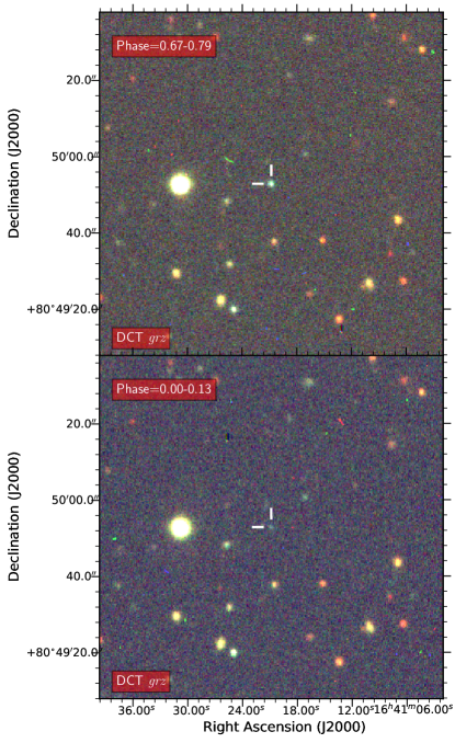
Figure 3: Composite rgb images of PSR J1641+8049, taken with the DCT’s LMI at two different orbital phases: 0.67–0.79 (close to photometric maximum) at the top, and 0.00-0.13 (close to photometric minimum) at the bottom. The composites are made from the $g$, $r$, and $z$ filters. The position of PSR J1641+8049 is indicated with the ticks toward the center: the astrometric uncertainties are dominated by the astrometric calibration of the optical images, which has uncertainties of roughly $0\farcs 2$. The image are $1.5\arcmin$ on a side, with north up and east to the left.

Based on positional agreement and strong photometric variability tied to the orbital period, we can be certain that we have identified the optical counterpart of PSR J1641+8049. Future observations and analysis will enable us to determine the range of radii and effective temperatures for the companion and use to those to constrain the mass of the pulsar and inclination of the binary system (e.g. Antoniadis et al., 2013).

5.3.6 PSR J1628+4406: A New Mode Changing Pulsar

PSR J1628+4406 has two emission modes, distinguished by differences in the amplitude of its pulse profile components (see Figure 9). In the first mode, the main pulse has two components with similar amplitudes (the leading component, i.e. leftward in Figure 9, is somewhat weaker than the trailing component), and there is a strong interpulse separated by $180\arcdeg$ in pulse phase from the trailer component of the main pulse. This general description of Mode 1 holds in both the $350\;\textrm{MHz}$ and $820\;\textrm{MHz}$ bands. In the $148\;\textrm{MHz}$ band observed with LOFAR, the leading component of the main pulse is blended with the trailing component but, given the asymmetry in the profile, the leading component seems to be much weaker. In the second mode, the amplitude of the leading component of the main pulse is greatly reduced and the interpulse nearly vanishes, though it is still visible when several observations in this mode are summed together. Each component remains at the same pulse phase in both modes.

Figure 4: A phase-time plot of J1628+4406 from MJD 56639 as observed by LOFAR. The pulsar experiences a significant drop in flux for 15 minutes but does not appear to change modes. No other similar events were observed.

We observed PSR J1628+4406 for a total of $48091\;\textrm{s}$ during our timing campaign, split between the $148\;\textrm{MHz}$ LOFAR band (where the vast majority of the observations were made), and the $350\;\textrm{MHz}$ and $820\;\textrm{MHz}$ bands of the GBT. Of this, the pulsar spent $33156\;\textrm{s}$ (70%) in Mode 1 while the remaining time ($14574\;\textrm{s}$; 30%) was spent in Mode 2. We never witnessed a transition between modes during an observation, but we did observe a single event in which the pulsar significantly dropped in flux across both profile components for approximately 15 minutes before recovering to its prior state (see Fig. 4). There is no record of an instrumental failure that would account for this drop in flux, nor was there indication of Solar activity that might cause ionospheric changes that would impact the observation at this level, so the flux change would appear to be a genuine phenomenon in this pulsar.

5.3.7 PSR J2123+5434: A 138-ms Pulsar with a Low Magnetic Field

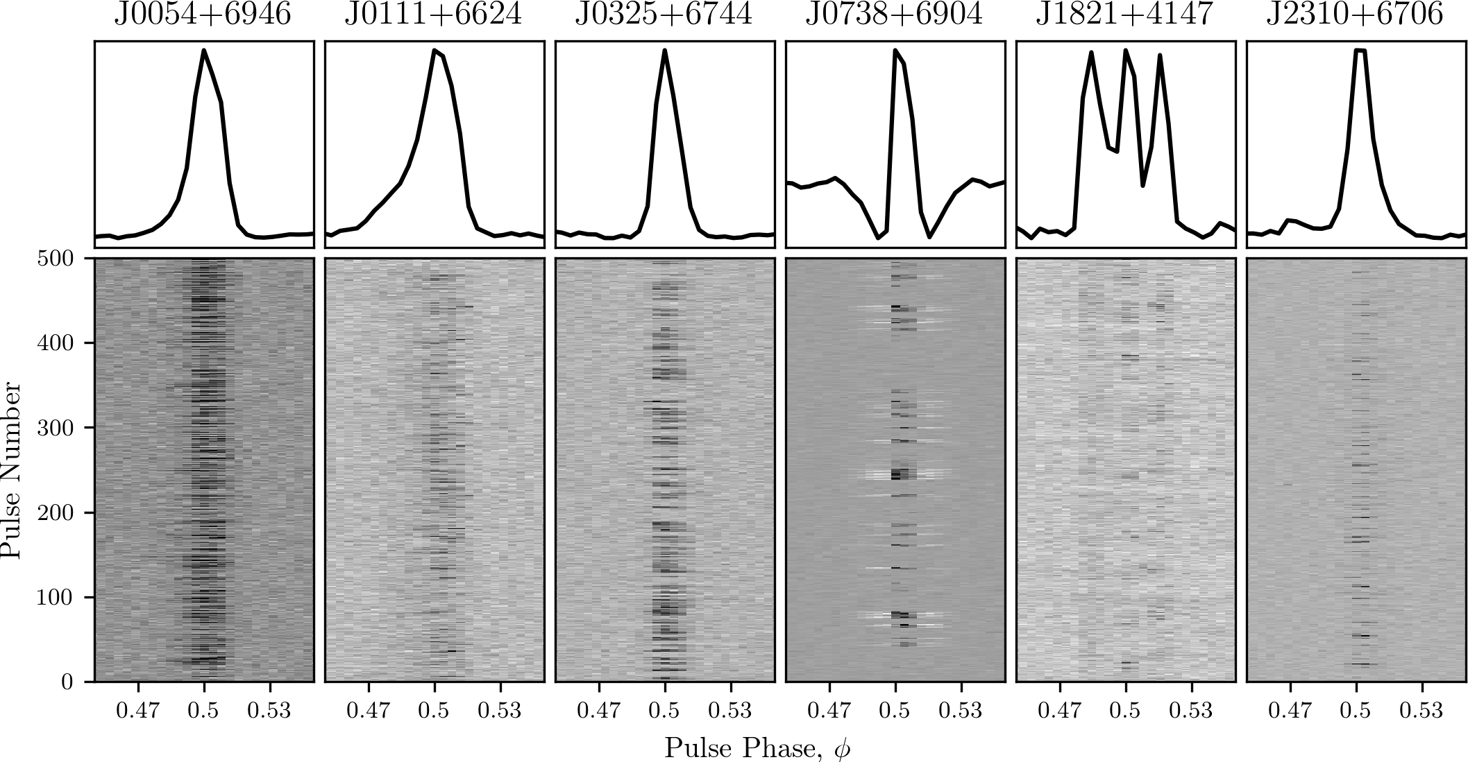
Figure 5: Preliminary single pulse analysis for six GBNCC nulling pulsars with existing timing solutions. All data were taken at $820\;\textrm{MHz}$. For each source, 500 pulses are plotted in the bottom panels to show nulling behavior; folded profiles are shown in the top panels, corresponding to the same duration of pulse phase ($0.45<\phi<0.55$). The apparent drop in flux on either side of the profile in PSR J0738+6904 is an artifact affecting subbanded data of bright pulsars. Since it is clear when the pulsar is in an ON or OFF state, we do not expect it to bias the results of our nulling analysis.

At the completion of our timing program, our timing solution for PSR J2123+5434 did not constrain $\dot{P}$. Therefore, we obtained additional observations for this pulsar through our survey program about 3 years after the initial program, giving us a total time span of 4 years. These additional observations enabled a $\dot{P}$ measurement of $1.7(1)\times 10^{-19}$, implying a surface magnetic field of $B_{\rm surf}=5.0(1)\times 10^{9}\;\textrm{G}$. These values are smaller than any known pulsar with a period $>100\;\textrm{ms}$ that has a constrained $\dot{P}$ measurement. Figure 1 shows the location of PSR J2123+5434 in the $P$-$\dot{P}$ plane in relation to the pulsars in the ATNF pulsar catalog. The expected change in $\dot{P}$ due to Galactic motion for PSR J2123+5434 (using the DM-derived distance of $2.1\;\textrm{kpc}$ (Cordes & Lazio, 2002)) is about $-2.3\times 10^{-20}$. After applying this correction, PSR J2123+5434 remains an outlier in comparison to the typical pulsar. A potential explanation for PSR J2123+5434’s anomolously low $\dot{P}$ is that it was partially recycled by a high mass companion star that later underwent a supernova, disrupting the system. Alternatively, the pulsar may be in a very wide binary, in which case we could be observing orbital phases in which the pulsar is accelerating towards the Earth, inducing a Doppler $\dot{P}<0$ (e.g. PSR J1024$-$0719 Kaplan et al., 2016; Bassa et al., 2016). We examined archival infrared and optical data at the timing position of J2123+5434, but did not identify a counterpart at any wavelength.

6 Nulling and Intermittent Pulsars

Given the rarity of the phenomenon, nulling studies typically characterize pulsars by their “nulling fractions” (NFs; the fraction of time spent in a null state) and look for correlations between NF and other measured/derived parameters like spin period, characteristic age, and profile morphology (e.g. Ritchings, 1976; Rankin, 1986; Biggs, 1992; Vivekanand, 1995; Wang et al., 2007).

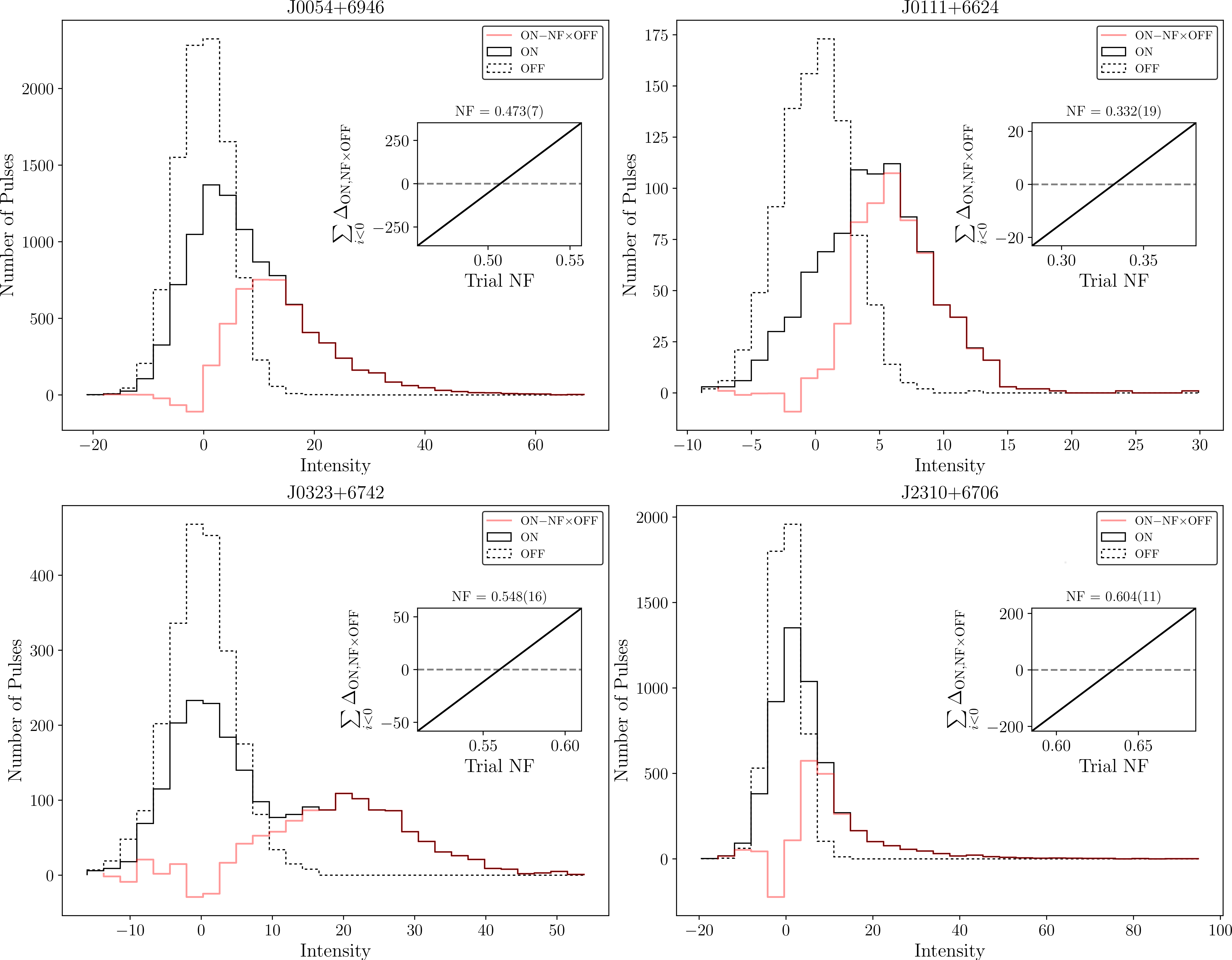
Figure 6: Histograms of summed intensities in ON/OFF windows for PSRs J0054+6946 (a), J0111+6624 (b), J0323+6742 (c), and J2310+6706 (d) are shown with solid/dashed lines, respectively. Inset in each panel: plots showing the difference, ON$-$NF$\times$OFF (summed over bins with intensity $<0$) versus trial NF values. The red line shows ON$-$NF$\times$OFF for the best NF value (where the summed difference is closest to zero).

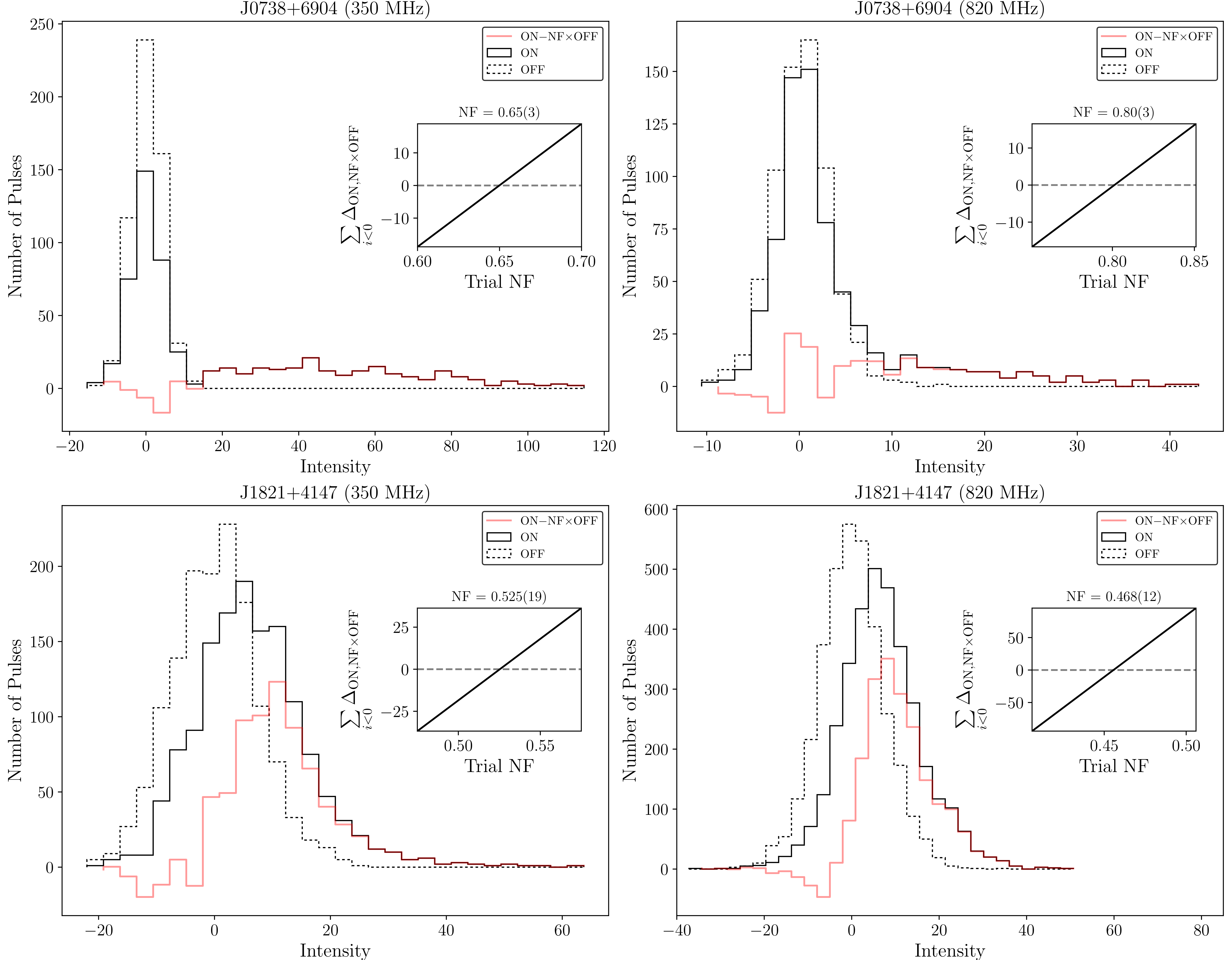
Figure 7: Histograms of summed intensities in ON/OFF windows for PSRs J0738+6904 (350 MHz) (a), J0738+6904 (820 MHz) (b), J1821+4147 (350 MHz) (c), and J1821+4147 (820 MHz) (d) are shown with solid/dashed lines, respectively. Inset in each panel: plots showing the difference, ON$-$NF$\times$OFF (summed over bins with intensity $<0$) versus trial NF values. The red line shows ON$-$NF$\times$OFF for the best NF value (where the summed difference is closest to zero).

To conduct an initial census of nulling pulsars among the discoveries described in this paper, we visually inspected each pulsar’s discovery plot and took note of sources that exhibited obvious intensity variations as a function of time, resulting in 19 nulling candidates. We followed a procedure similar to that described in Ritchings (1976) to investigate which (if any) of these pulsars exhibited measurable nulling behavior. Here, we describe the procedure used to process and analyze data for each candidate in order to identify nulling pulsars in this sample.

Once this initial selection was made, we used timing data (at both $350$ and $820\;\textrm{MHz}$) on all of the candidate nullers to confirm or reject them as nulling pulsars and measure nulling fractions where appropriate. Subbanded timing data were dedispersed and folded modulo the pulsar’s spin period, resulting in files containing sub-integrations equivalent in length to the pulsar’s spin period and 64 frequency channels across the band. RFI was removed interactively with pazi, part of the PSRCHIVE pulsar processing software package (Hotan et al., 2004). After downsampling all cleaned detections in time and frequency, the resulting folded profile was used to determine ON/OFF-pulse windows of equal size. In most cases, ON/OFF windows spanned $\lesssim 15$ bins, or about 5% of a full rotation (256 bins). The ON window was centered on the ON-pulse region and the OFF window was fixed 100 bins away, sampling baseline noise.

Cleaned data were downsampled in frequency and remaining bins outside both ON/OFF windows were used to subtract a DC offset (mean value) from single pulses; any remaining low-frequency noise was also removed during this stage by fitting out a 6th-order polynomial from the baseline. Examples of resulting single pulse intensities (and folded profiles) are shown in Figure 5. Summed intensities were recorded for each single pulse in both ON and OFF windows, then binned over intensity to create histograms (see Figures 6 and 7) for each window. In order to identify pulsars exhibiting some form of nulling behavior, we looked for sources with ON histograms that showed both measurable single pulse emission (a tail or positive distribution of ON intensities) and a distribution of null pulses centered on zero intensity, inside the envelope of the OFF histogram (see panel for PSR J0323+6742 in Figure 6 for a canonical example).

Of the 19 candidates for which we carried out this analysis, eight pulsars (group A; PSRs J0612+3721, J1859+7654, J1941+4320, J1954+4357, J2137+6428, J2228+6447, J2312+6931, and J2351+8533) were too weak to see single pulses and, therefore, results were inconclusive. Five others (group B; PSRs J0137+6349, J0335+6623, J0944+4106, J1059+6459, and J1647+6609) showed obvious single pulse emission, but no null distribution was apparent in any of their ON histograms using existing data. Based on our analysis, pulsars from group A have single pulse emission below our detection threshold, but because of intensity variability apparent in their discovery plots, we may be able to carry out a similar analysis by summing groups of single pulses (as in Wang et al., 2007) and looking for longer nulls. Pulsars from group B may have extremely low NFs, which may be detectable with extended datasets.

The remaining six pulsars from the original candidate list (PSRs J0054+6946, J0111+6624, J0323+6742, J0738+6904, J1821+4147, and J2310+6706) were identified as new nulling pulsars (see Figure 5 for profiles and examples of their single pulse behavior. Using their ON/OFF histograms (see Figures 6 and 7), we computed preliminary NFs and found values between 0.33–0.80. For PSRs J0738+6904 and J1821+4147, timing data from multiple frequencies ($350$ and $820\;\textrm{MHz}$) allowed us to compare nulling behavior across frequency; based on preliminary results shown in Figure 7, we found similar ON distributions and NF values, independent of observing frequency, as also found by Gajjar et al. (2014) on 3 nulling pulsars.

An analysis that will select nulling pulsars using all existing timing data with an improved method that uses Gaussian mixture models and accounts for the effects of scintillation is underway. Also of interest in a future study would be a detailed comparison between these new sources and the rest of the known nulling population as well as predictions about the underlying nulling population, given the relatively complete and unbiased nature of the GBNCC survey.

7 Optical Constraints

Table 8: Optical Counterpart Limits

Source	Companion Massa	Companion Type	Teff	Constraining Filter	WD Age
	(M⊙)		(K)	(g/r/i/z)	(Gyr)
J0740+6620	00.20	He WD	0$<4200$	i	0$>3.2$
	00.23		0$<4400$		0$>4.0$
J1125+7819	00.29	He WD	0$<4400$	i	0$>3.3$
	00.33		0$<3500$		0$>5.6$
J1938+6604	00.87	CO WD	0$<20000$	g	0$>0.179$
	01.04		0$<25000$		0$>0.118$

Note. — We use the larger of the DM-inferred distance from either the NE2001 or YMW16 models in setting limits.

Each of the MSPs with a binary companion and nearly circular orbit (see Table 5) most likely has a WD companion. For all of them, we looked for optical counterparts using data from the PanSTARRS $3\pi$ Steradian Survey (Chambers et al., 2016). By manually inspecting individual (grizy) bands from the PanSTARRS survey’s PS1 data release, we found a counterpart for PSR J1641+8049 (§5.3.5), but none were found for the three other sources. For non-detections, we used the minimum/median companion masses derived from the systems’ binary parameters (see Table 8) and the average 5-$\sigma$ magnitude lower limits for the PS1 grizy bands (23.3, 23.2, 23.1, 22.3, and 21.4, respectively; Chambers et al., 2016) to place constraints on the properties of each MSP’s WD companion. Based on computed minimum companion masses, PSRs J0740+6620 and J1125+7819 likely have He WD companions and PSR J1938+6604, a CO WD companion.

Reddening was estimated using a 3-D map of interstellar dust reddening by Green et al. (2015), the pulsar’s sky position and $D_{\rm DM}$ (see Tables 4 and 5; we used the larger of the DM-inferred distances from the NE2001 or YMW16 models to calculate the most conservative limits). These values were converted to extinctions in each PS1 band using Table 6 from Schlafly & Finkbeiner (2011). Resulting magnitude limits were translated to upper limits on WD effective temperatures ($T_{\rm eff}$) using models for WD mass, radius and temperature from Istrate et al. (2016). The best WD $T_{\rm eff}$ constraints are listed for each pulsar’s minimum/median companion mass in Table 8, along with the PS1 bands providing those constraints, and modeled WD cooling ages (Istrate et al., 2016). Because of its significantly higher companion mass, we used different models (Tremblay et al., 2011; Bergeron et al., 2011) to place constraints on PSR J1938+6604’s CO WD, but otherwise followed the same procedure described here.

Based on mass and temperature constraints, both PSRs J0740+6620 and J1125+7819 have cool He WD companions; for these systems, a correlation between $P_{\rm b}$ and WD mass is expected (Savonije, 1987; Tauris & Savonije, 1999) and the $(P_{\rm b},m_{\rm WD})$-relationship predicts companion masses of 0.25 $\mathrm{M_{\sun}}$and 0.28 $\mathrm{M_{\sun}}$, respectively. These are consistent with the minimum companion masses for these systems.

8 Conclusion

We present here complete timing solutions for 45 new pulsars discovered by the GBNCC survey. The highlights include two new PTA pulsars that are being used in an effort to detect low-frequency GWs, several intermittent pulsars, a mode changing pulsar, and five binary pulsars. Among the binary pulsars are a new DNS system, IMBP, and black widow.

These results demonstrate the importance of long-term pulsar timing, as many properties, such as spin-down and proper motion, can only be measured with data spanning a year or more. We continue to observe select sources to improve the measurements of proper motion and some binary parameters. We also are observing approximately 100 additional pulsars discovered in the GBNCC survey, which will be presented in future work. Given our current estimate of survey yield, we expect to discover an additional few dozen long-period pulsars and of order 5–10 MSPs before the survey is completed.

Figure 8: Post-fit timing residuals for the 45 pulsars presented here. Colors correspond to different observing bands: $148\;\textrm{MHz}$ (blue) $350\;\textrm{MHz}$ (orange), $820\;\textrm{MHz}$ (dark green), $1500\;\textrm{MHz}$ (pink), and $2000\;\textrm{MHz}$ (brown). Note that vertical and horizontal scales differ for each pulsars.

Figure 8: Post-fit timing residuals for the 45 pulsars presented here. Colors correspond to different observing bands: $148\;\textrm{MHz}$ (blue) $350\;\textrm{MHz}$ (orange), $820\;\textrm{MHz}$ (dark green), $1500\;\textrm{MHz}$ (pink), and $2000\;\textrm{MHz}$ (brown). Note that vertical and horizontal scales differ for each pulsars.

Figure 8: Post-fit timing residuals for the 45 pulsars presented here. Colors correspond to different observing bands: $148\;\textrm{MHz}$ (blue) $350\;\textrm{MHz}$ (orange), $820\;\textrm{MHz}$ (dark green), $1500\;\textrm{MHz}$ (pink), and $2000\;\textrm{MHz}$ (brown). Note that vertical and horizontal scales differ for each pulsars.

Figure 8: Post-fit timing residuals for the 45 pulsars presented here. Colors correspond to different observing bands: $148\;\textrm{MHz}$ (blue) $350\;\textrm{MHz}$ (orange), $820\;\textrm{MHz}$ (dark green), $1500\;\textrm{MHz}$ (pink), and $2000\;\textrm{MHz}$ (brown). Note that vertical and horizontal scales differ for each pulsars.

Figure 8: Post-fit timing residuals for the 45 pulsars presented here. Colors correspond to different observing bands: $148\;\textrm{MHz}$ (blue) $350\;\textrm{MHz}$ (orange), $820\;\textrm{MHz}$ (dark green), $1500\;\textrm{MHz}$ (pink), and $2000\;\textrm{MHz}$ (brown). Note that vertical and horizontal scales differ for each pulsars.

Figure 8: Post-fit timing residuals for the 45 pulsars presented here. Colors correspond to different observing bands: $148\;\textrm{MHz}$ (blue) $350\;\textrm{MHz}$ (orange), $820\;\textrm{MHz}$ (dark green), $1500\;\textrm{MHz}$ (pink), and $2000\;\textrm{MHz}$ (brown). Note that vertical and horizontal scales differ for each pulsars.

Figure 8: Post-fit timing residuals as a function of orbital phase for the binary pulsars presented here. Colors correspond to different observing bands: $148\;\textrm{MHz}$ (blue) $350\;\textrm{MHz}$ (orange), $820\;\textrm{MHz}$ (dark green), $1500\;\textrm{MHz}$ (pink), and $2000\;\textrm{MHz}$ (brown). Note that vertical scale differs for each pulsars.

Figure 9: Average pulse profiles for the 45 pulsars presented here. Data from all available observing bands are presented. All profiles have been rotated $180\arcdeg$ from the zero-point pulse phase reference.

References

- Ahn et al. (2014) Ahn, C. P., Alexandroff, R., Allende Prieto, C., et al. 2014, ApJS, 211, 17
- Antoniadis et al. (2016) Antoniadis, J., Tauris, T. M., Ozel, F., et al. 2016, ArXiv e-prints, arXiv:1605.01665
- Antoniadis et al. (2013) Antoniadis, J., Freire, P. C. C., Wex, N., et al. 2013, Science, 340, 448
- Arzoumanian et al. (2018) Arzoumanian, Z., Brazier, A., Burke-Spolaor, S., et al. 2018, ApJS, 235, 37
- Backer (1970) Backer, D. C. 1970, Nature, 228, 42
- Bassa et al. (2016) Bassa, C. G., Janssen, G. H., Stappers, B. W., et al. 2016, MNRAS, 460, 2207
- Bergeron et al. (2011) Bergeron, P., Wesemael, F., Dufour, P., et al. 2011, ApJ, 737, 28
- Bertin (2006) Bertin, E. 2006, in Astronomical Society of the Pacific Conference Series, Vol. 351, Astronomical Data Analysis Software and Systems XV, ed. C. Gabriel, C. Arviset, D. Ponz, & S. Enrique, 112
- Bertin & Arnouts (1996) Bertin, E., & Arnouts, S. 1996, A&AS, 117, 393
- Bhattacharyya & Nityananda (2008) Bhattacharyya, B., & Nityananda, R. 2008, MNRAS, 387, 273
- Biggs (1992) Biggs, J. D. 1992, ApJ, 394, 574
- Camilo et al. (2001) Camilo, F., Lyne, A. G., Manchester, R. N., et al. 2001, ApJ, 548, L187
- Camilo et al. (2015) Camilo, F., Kerr, M., Ray, P. S., et al. 2015, ApJ, 810, 85
- Capitaine et al. (2003) Capitaine, N., Wallace, P. T., & Chapront, J. 2003, A&A, 412, 567
- Chambers et al. (2016) Chambers, K. C., Magnier, E. A., Metcalfe, N., et al. 2016, ArXiv e-prints, arXiv:1612.05560
- Chawla et al. (2017) Chawla, P., Kaspi, V. M., Josephy, A., et al. 2017, ArXiv e-prints, arXiv:1701.07457
- Cordes & Lazio (2002) Cordes, J. M., & Lazio, T. J. W. 2002, ArXiv Astrophysics e-prints, astro-ph/0207156
- de Jager et al. (1989) de Jager, O. C., Raubenheimer, B. C., & Swanepoel, J. W. H. 1989, A&A, 221, 180
- Demorest et al. (2010) Demorest, P. B., Pennucci, T., Ransom, S. M., Roberts, M. S. E., & Hessels, J. W. T. 2010, Nature, 467, 1081
- Espinoza et al. (2013) Espinoza, C. M., Guillemot, L., Çelik, Ö., et al. 2013, MNRAS, 430, 571
- Ferdman et al. (2013) Ferdman, R. D., Stairs, I. H., Kramer, M., et al. 2013, ApJ, 767, 85
- Fruchter et al. (1988) Fruchter, A. S., Stinebring, D. R., & Taylor, J. H. 1988, Nature, 333, 237
- Gajjar (2017) Gajjar, V. 2017, ArXiv e-prints, arXiv:1706.05407
- Gajjar et al. (2014) Gajjar, V., Joshi, B. C., Kramer, M., Karuppusamy, R., & Smits, R. 2014, ApJ, 797, 18
- Gonzalez et al. (2011) Gonzalez, M. E., Stairs, I. H., Ferdman, R. D., et al. 2011, ApJ, 743, 102
- Green et al. (2015) Green, G. M., Schlafly, E. F., Finkbeiner, D. P., et al. 2015, ApJ, 810, 25
- Hobbs (2013) Hobbs, G. 2013, Classical and Quantum Gravity, 30, 224007
- Hobbs et al. (2005) Hobbs, G., Lorimer, D. R., Lyne, A. G., & Kramer, M. 2005, MNRAS, 360, 974
- Hotan et al. (2004) Hotan, A. W., van Straten, W., & Manchester, R. N. 2004, PASA, 21, 302
- Istrate et al. (2016) Istrate, A. G., Marchant, P., Tauris, T. M., et al. 2016, A&A, 595, A35
- Kaplan et al. (2016) Kaplan, D. L., Kupfer, T., Nice, D. J., et al. 2016, ApJ, 826, 86
- Karako-Argaman et al. (2015) Karako-Argaman, C., Kaspi, V. M., Lynch, R. S., et al. 2015, ApJ, 809, 67
- Kawash et al. (2018) Kawash, A. M., McLaughlin, M. A., Kaplan, D. L., et al. 2018, ApJ, 857, 131
- Kiziltan et al. (2013) Kiziltan, B., Kottas, A., De Yoreo, M., & Thorsett, S. E. 2013, ApJ, 778, 66
- Kondratiev et al. (2016) Kondratiev, V. I., Verbiest, J. P. W., Hessels, J. W. T., et al. 2016, A&A, 585, A128
- Kramer & Champion (2013) Kramer, M., & Champion, D. J. 2013, Classical and Quantum Gravity, 30, 224009
- Kramer et al. (2006) Kramer, M., Stairs, I. H., Manchester, R. N., et al. 2006, Science, 314, 97
- Lange et al. (2001) Lange, C., Camilo, F., Wex, N., et al. 2001, MNRAS, 326, 274
- Lattimer & Prakash (2004) Lattimer, J. M., & Prakash, M. 2004, Science, 304, 536
- Lyne et al. (2010) Lyne, A., Hobbs, G., Kramer, M., Stairs, I., & Stappers, B. 2010, Science, 329, 408
- Manchester et al. (2005) Manchester, R. N., Hobbs, G. B., Teoh, A., & Hobbs, M. 2005, AJ, 129, 1993
- Manchester & IPTA (2013) Manchester, R. N., & IPTA. 2013, Classical and Quantum Gravity, 30, 224010
- Matthews et al. (2016) Matthews, A. M., Nice, D. J., Fonseca, E., et al. 2016, ApJ, 818, 92
- McLaughlin (2013) McLaughlin, M. A. 2013, Classical and Quantum Gravity, 30, 224008
- McLaughlin et al. (2006) McLaughlin, M. A., Lyne, A. G., Lorimer, D. R., et al. 2006, Nature, 439, 817
- Morris et al. (2002) Morris, D. J., Hobbs, G., Lyne, A. G., et al. 2002, MNRAS, 335, 275
- Nice & Taylor (1995) Nice, D. J., & Taylor, J. H. 1995, ApJ, 441, 429
- Özel et al. (2012) Özel, F., Psaltis, D., Narayan, R., & Santos Villarreal, A. 2012, ApJ, 757, 55
- Phinney et al. (1988) Phinney, E. S., Evans, C. R., Blandford, R. D., & Kulkarni, S. R. 1988, Nature, 333, 832
- Rankin (1986) Rankin, J. M. 1986, ApJ, 301, 901
- Ransom et al. (2002) Ransom, S. M., Eikenberry, S. S., & Middleditch, J. 2002, AJ, 124, 1788
- Ransom et al. (2011) Ransom, S. M., Ray, P. S., Camilo, F., et al. 2011, ApJ, 727, L16
- Ritchings (1976) Ritchings, R. T. 1976, MNRAS, 176, 249
- Roberts (2013) Roberts, M. S. E. 2013, in IAU Symposium, Vol. 291, Neutron Stars and Pulsars: Challenges and Opportunities after 80 years, ed. J. van Leeuwen, 127–132
- Savonije (1987) Savonije, G. J. 1987, Nature, 325, 416
- Schlafly & Finkbeiner (2011) Schlafly, E. F., & Finkbeiner, D. P. 2011, ApJ, 737, 103
- Shklovskii (1970) Shklovskii, I. S. 1970, Soviet Ast., 13, 562
- Siemens et al. (2013) Siemens, X., Ellis, J., Jenet, F., & Romano, J. D. 2013, Classical and Quantum Gravity, 30, 224015
- Splaver et al. (2002) Splaver, E. M., Nice, D. J., Arzoumanian, Z., et al. 2002, ApJ, 581, 509
- Stovall et al. (2014) Stovall, K., Lynch, R. S., Ransom, S. M., et al. 2014, ApJ, 791, 67
- Tauris & Savonije (1999) Tauris, T. M., & Savonije, G. J. 1999, A&A, 350, 928
- Taylor (1992) Taylor, J. H. 1992, Royal Society of London Philosophical Transactions Series A, 341, 117
- Taylor & Weisberg (1989) Taylor, J. H., & Weisberg, J. M. 1989, ApJ, 345, 434
- Tody (1986) Tody, D. 1986, in Proc. SPIE, Vol. 627, Instrumentation in astronomy VI, ed. D. L. Crawford, 733
- Tody (1993) Tody, D. 1993, in Astronomical Society of the Pacific Conference Series, Vol. 52, Astronomical Data Analysis Software and Systems II, ed. R. J. Hanisch, R. J. V. Brissenden, & J. Barnes, 173
- Toscano et al. (1999) Toscano, M., Sandhu, J. S., Bailes, M., et al. 1999, MNRAS, 307, 925
- Tremblay et al. (2011) Tremblay, P.-E., Bergeron, P., & Gianninas, A. 2011, ApJ, 730, 128
- van Haarlem et al. (2013) van Haarlem, M. P., Wise, M. W., Gunst, A. W., et al. 2013, A&A, 556, A2
- Vivekanand (1995) Vivekanand, M. 1995, MNRAS, 274, 785
- Wang et al. (2007) Wang, N., Manchester, R. N., & Johnston, S. 2007, MNRAS, 377, 1383
- Weisberg et al. (2010) Weisberg, J. M., Nice, D. J., & Taylor, J. H. 2010, ApJ, 722, 1030
- Wu et al. (2012) Wu, J. H. K., Kong, A. K. H., Huang, R. H. H., et al. 2012, ApJ, 748, 141
- Yao et al. (2017) Yao, J. M., Manchester, R. N., & Wang, N. 2017, ApJ, 835, 29
- Zhu et al. (2014) Zhu, W. W., Berndsen, A., Madsen, E. C., et al. 2014, ApJ, 781, 117