Entanglement Content of Quasi-Particle Excitations

Abstract

We investigate the quantum entanglement content of quasi-particle excitations in extended many-body systems. We show that such excitations give an additive contribution to the bi-partite von Neumann and Rényi entanglement entropies that takes a simple, universal form. It is largely independent of the momenta and masses of the excitations, and of the geometry, dimension and connectedness of the entanglement region. The result has a natural quantum information theoretic interpretation as the entanglement of a state where each quasi-particle is associated with two qubits representing their presence within and without the entanglement region, taking into account quantum (in)distinguishability. This applies to any excited state composed of finite numbers of quasi-particles with finite De Broglie wavelengths or finite intrinsic correlation length. We derive this result analytically in one-dimensional massive bosonic and fermionic free field theories and for simple setups in higher dimensions. We provide numerical evidence for the harmonic chain and the two-dimensional harmonic lattice in all regimes where excitations have quasi-particle properties. Finally, we provide supporting calculations for integrable spin chain models and other situations without particle production. Our results point to new possibilities for creating entangled states using many-body quantum systems.

Introduction.— Measures of entanglement, such as the entanglement entropy (EE) bennet and entanglement negativity VW ; ZHSL ; ple ; erratumple ; Eisert ; Eisert2 , have attracted much attention in recent years, both theoretically EERev1 ; specialissue ; EERev2 and experimentally Greiner1 ; Greiner2 . Quantum entanglement encodes correlations between degrees of freedom associated to independent factors of the Hilbert space, and as such, it separates quantum correlations from the particularities of observables. As a consequence, the entanglement in extended systems encodes, in a natural fashion, universal properties of the state. For instance, at criticality, the entanglement of ground states provides an efficient measure of universal properties of quantum phase transitions, such as the (effective) central change of the corresponding conformal field theory (CFT) and the primary operator content CallanW94 ; HolzheyLW94 ; latorre1 ; Latorre2 ; Calabrese:2004eu ; Calabrese:2005in ; disco1 ; negativity1 ; negativity2 ; BCDLR . Near criticality, it is universally controlled by the masses of excitations entropy ; next ; ourneg . In states that are highly excited, with finite energy densities, the entanglement is known to give rise to local thermalisation effects: this is at the heart of the eigenstate thermalisation hypothesis ETH1 ; ETH2 ; ETH3 ; ETH4 ; ETH5 , as the large entanglement between local degrees of freedom and the rest of the system effectively generates a Gibbs ensemble (in the case of integrable systems, a generalized Gibbs ensemble). The entanglement effects of a finite number of excitations are less known. Some results are available in critical systems: using the methods of Holzhey, Larsen and Wilczek HolzheyLW94 , combining a geometric description with Riemann uniformization techniques in CFT it was shown in german1 ; german2 that certain excitations, with energies tending to zero in the large volume limit, correct the ground state entanglement by power laws in the ratio of length scales. Various few-particle states have also been studied in special cases of integrable spin chains Vincenzo ; ln2 ; SS ; Berko ; Vincenzo2 .

In this paper we propose a universal formula, with a simple quantum information theoretic interpretation, for the entanglement content of states with well-defined quasi-particle excitations. For this purpose, we study a variety of extended systems of different dimensions. We consider the von Neumann and Rényi EEs: these are measures of the amount of quantum entanglement, in a pure quantum state, between the degrees of freedom associated to two sets of independent observables whose union is complete on the Hilbert space. We use the setup where the Hilbert space is factorised as ${\cal H}_{A}\otimes{\cal H}_{B}$, according to two complementary spatial regions $A$ and $B$, of typical length scales $\ell_{A}$ and $\ell_{B}$, respectively (for dimensions higher than one, we can think of these as the diameters of the regions under consideration). The regions can be of generic geometry and connectedness. Quasi-particle excitations arise naturally in massive quantum field theory (QFT), where irreducible representations of the Poincaré group are identified with relativistic particles. We first consider excited states of the massive free real boson and free Majorana fermion models, formed of finite numbers $k$ of particles, at various momenta. We use techniques based on form factors of branch point twist fields in 1+1 dimensions as introduced in entropy , and dimensional reduction methods KG to access simple entanglement regions in higher dimensions. More generally, excitations in the harmonic chain and in higher-dimensional harmonic lattices can be interpreted as being composed of quasi-particles whenever the correlation length $\xi$ is small enough, $\xi\ll{\rm min}(\ell_{A},\ell_{B})$, or the maximal De Broglie wavelength of the particles $\zeta={\rm max}\{2\pi/|\vec{p}_{i}|\}$, where $\vec{p}_{i}$ are the particles’ momenta, is small enough, $\zeta\ll{\rm min}(\ell_{A},\ell_{B})$. This includes the large-momenta region of the chain’s or lattice’s CFT regime (beyond the applicability of the results of german1 ; german2 ), as well as the non-universal regime, beyond QFT and CFT. We then study the harmonic chain and two-dimensional lattice numerically. Quasi-particles also arise naturally in Bethe ansatz integrable models, where the conditions $\xi\ll{\rm min}(\ell_{A},\ell_{B})$ and $\zeta\ll{\rm min}(\ell_{A},\ell_{B})$ can be given precise meanings. We study few-particle excitations in generic states of the Bethe form. In this case, the calculation is elementary, and complements some of the calculations done in Vincenzo . Zamolodchikov’s ideas underpinning the thermodynamic Bethe ansatz tba1 ; tba2 in fact suggest that the same calculation should also give the correct answer in massive integrable QFT, thus including the effects of interactions. In all cases, we find a universal result in the limit ${\rm min}(\xi,\zeta)\ll{\rm min}(\ell_{A},\ell_{B})$, independent of the model studied, of the connectedness or shape of the entanglement region, and of the dimension. The result extends the “semiclassical” form discussed in the context of spin chains in Vincenzo . It has a very natural qubit interpretation where qubits representing the particles are entangled according to the particles’ distribution in space, taking into account quantum indistinguishability in the bosonic case. The qubit interpretation indicates that quasi-particle excitations in many-body models may provide a simple way of generating entangled states with easily adjustable parameters.

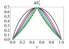
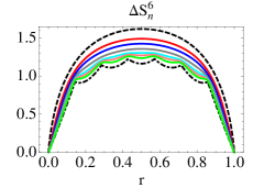
Figure 1: The functions (3) and (8) for $k=1,6$ and $n=2,3,5,8,11,17$ and the limits $n\rightarrow 1$ (von Neumann) and $n\rightarrow\infty$ (single-copy). The outer-most curve is the von Neumann entropy and the inner-most curve is the single-copy entropy.

Results.— Consider a bi-partition of a system $C=A\cup B$ in state $|\Psi\rangle$ composed of a number $k$ of quasi-particles. In infinite volume, the notion of quasi-particles is very natural via the theory of scattering states poles ; qft , and one expects that in finite but large volumes there are corresponding excited states, unambiguously defined up to exponentially decaying corrections in the volume. We define the reduced density matrix associated to subsystem $A$ as $\rho_{A}={\rm Tr}_{B}(|\Psi\rangle\langle\Psi|)$. The Rényi EE is the Rényi entropy of this reduced density matrix,

$$S_{n}^{\Psi}(A,B)=\frac{\log{\rm Tr}\rho_{A}^{n}}{1-n}.$$ (1)

From (1) we may compute the von Neumann EE as $S^{\Psi}_{1}(A,B):=\lim_{n\rightarrow 1}S_{n}^{\Psi}(A,B)$ and the so-called single-copy entropy EC ; PZ ; DD as $S_{\infty}^{\Psi}(A,B):=\lim_{n\rightarrow\infty}S_{n}^{\Psi}(A,B)$. For large system size and fixed entanglement region, one expects the entanglement entropies to tend to those of the ground state. We therefore concentrate on the nontrivial limit where both the full system $C$ and the entanglement region $A$ are large, scaled simultaneously, $A\mapsto\lambda A$ and $B\mapsto\lambda B$. Let $r={\rm Vol}_{d}\,(A)/{\rm Vol}_{d}\,(C)$ be the ratio of the $d$-dimensional hypervolume of the region to that of the system. We compute the difference $\Delta{S}_{n}^{\Psi}(A,B)=S_{n}^{\Psi}(A,B)-S_{n}^{0}(A,B)$ between the Rényi entropy in the excited state $|\Psi\rangle$ and in the ground (vacuum) state $|0\rangle$, in this limit,

$$\Delta{S}_{n}^{\Psi}(r):=\lim_{\lambda\to\infty}\Delta{S}_{n}^{\Psi}(\lambda A,\lambda B).$$ (2)

This is the contribution of the excitations to the entanglement, or “excess entanglement” as named in german1 ; german2 .

We find that for a wide variety of quantum systems, the results depend only on the proportion $r$ of the system’s volume occupied by the entanglement region, and are largely independent of the momenta of the quasi-particles. Suppose the state is formed of $k$ particles of equal momenta. Denoting $\Delta S_{n}^{\Psi}(r)=\Delta S_{n}^{k}(r)$, we find

$$\Delta{S}_{n}^{k}(r)=\frac{\log\sum\limits_{q=0}^{k}f_{q}^{k}(r)^{n}}{1-n},\ \Delta{S}^{k}_{1}(r)=-{\sum\limits_{q=0}^{k}f_{q}^{k}(r)\log f_{q}^{k}(r)}$$ (3)

with $f_{q}^{k}(r)=\left(\begin{array}[]{c}k\\ q\end{array}\right)r^{q}(1-r)^{k-q}$. For a state composed of $k$ particles divided into groups of $k_{i}$ particles of equal momenta $\vec{p}_{i}$, with $i=1,2,\ldots$ and $\sum_{i}k_{i}=k$, we denote $\Delta S_{n}^{\Psi}(r)=\Delta S_{n}^{k_{1},k_{2},\ldots}(r)$ and have

$$\Delta S_{n}^{k_{1},k_{2},\ldots}(r)=\sum_{i}\Delta{S}_{n}^{k_{i}}(r).$$ (4)

In particular, for $k$ particles of distinct momenta the result is $k$ times that for a single particle, which is

$$\Delta{S}_{n}^{1}(r) = \frac{\log(r^{n}+(1-r)^{n})}{1-n},$$

$$\Delta{S}^{1}_{1}(r) = -r\log r-(1-r)\log(1-r).$$ (5)

We observe that in all cases, the entanglement is maximal at $r=1/2$. For $k$ distinct-momenta particles, the maximum is $k\log 2$, while when some particles have coinciding momenta, the maximal value is smaller. Interestingly, single-copy entropies present non-analytic features. For distinct momenta, we have

$$\Delta{S}_{\infty}^{1}(r)=\left\{\begin{array}[]{ll}-\log(1-r)&\mathrm{for}\quad 0\leq r<\frac{1}{2}\\ -\log r&\mathrm{for}\quad\frac{1}{2}\leq r\leq 1.\end{array}\right.$$ (6)

Again, the result is just multiplied by $k$ for a state consisting of $k$ distinct-momentum particles. For equal momenta it is a function which is non-differentiable at $k$ points in the interval $r\in(0,1)$ (generalizing (6)). The positions of these cusps are given by the values

$$r=\frac{1+q}{1+k}\quad\mathrm{for}\quad q=0,\ldots,k-1,$$ (7)

and the single copy entropy is given by

$$\Delta{S}_{\infty}^{k}(r)=-\log f_{q}^{k}(r)\quad\mathrm{for}\quad\frac{q}{1+k}\leq r<\frac{1+q}{1+k}$$ (8)

and $q=0,\dots,k$.

The results take their full meaning under a quantum information theoretic interpretation that combines a “semiclassical” picture of particles with quantum indistinguishability. Consider a bi-partite Hilbert space ${\cal H}={\cal H}_{\rm int}\otimes{\cal H}_{\rm ext}$. Each factor ${\cal H}_{\rm int}\simeq{\cal H}_{\rm ext}$ is a tensor product $\otimes_{i}{\cal H}^{k_{i}}$ of Hilbert spaces ${\cal H}^{k_{i}}\simeq{\mathbb{C}}^{k_{i}+1}$ for $k_{i}$ indistinguishable qubits, with, as above, $\sum_{i}k_{i}=k$. We associate ${\cal H}_{\rm int}$ with the interior of the region $A$ and ${\cal H}_{\rm ext}$ with its exterior, and we identify the qubit state $1$ with the presence of a particle and $0$ with its absence. We construct the state $|\Psi_{\rm qb}\rangle\in{\cal H}$ under the picture according to which equal-momenta particles are indistinguishable, and a particle can lie anywhere in the full volume of the system with flat probability. That is, any given particle has probability $r$ of lying within $A$, and $1-r$ of lying outside of it. We make a linear combination of qubit states following this picture, with coefficients that are square roots of the total probability of a given qubit configuration, taking proper care of (in)distinguishability. For instance, for a single particle,

$$|\Psi_{\rm qb}\rangle=\sqrt{r}\;|1\rangle\otimes|0\rangle+\sqrt{1-r}\;|0\rangle\otimes|1\rangle$$ (9)

as either the particle is in the region, with probability $r$, or outside of it, with probability $1-r$. If two particles of coinciding momenta are present, then we have

$$|\Psi_{\rm qb}\rangle = \sqrt{r^{2}}\;|2\rangle\otimes|0\rangle+\sqrt{2r(1-r)}\;|1\rangle\otimes|1\rangle$$ (10)

$$+\,\sqrt{(1-r)^{2}}\;|0\rangle\otimes|2\rangle$$

as either the two particles are in the region, with probability $r^{2}$, or one is in the region and one outside of it (no matter which one), with probability $2r(1-r)$, or both are outside the region, with probability $(1-r)^{2}$. For two particles of different momenta,

$$|\Psi_{\rm qb}\rangle = \sqrt{r^{2}}\;|11\rangle\otimes|00\rangle+\sqrt{(1-r)^{2}}\;|00\rangle\otimes|11\rangle$$ (11)

$$+\,\sqrt{r(1-r)}\;(|10\rangle\otimes|01\rangle+|01\rangle\otimes|10\rangle)$$

counting the various ways two distinct particles can be distributed inside or outside the region. Higher-particle states can be constructed similarly. The results stated above are then equivalent to the identification $\Delta S_{n}^{\Psi}(r)=\Delta S_{n}^{\Psi_{\rm qb}}(r)$, where

$$\Delta S_{n}^{\Psi_{\rm qb}}(r)=\frac{\log{\rm Tr}\rho_{{\rm int}}^{n}}{1-n},\quad\rho_{{\rm int}}={\rm Tr}_{{\rm ext}}|\Psi_{\rm qb}\rangle\langle\Psi_{\rm qb}|.$$ (12)

Methods.— In general, the quantity $\Delta S_{n}^{\Psi}$ can be computed using the replica method CallanW94 ; HolzheyLW94 . In this context, one evaluates traces of powers of the reduced density matrix $\rho_{A}$. After reinterpretation of such traces, this boils down to ratios of expectation values of a twist operator, acting on a replica model composed of $n$ independent copies of the original theory. The operator $\mathbb{T}(A,B)$ acts as a cyclic permutation of the copies $i\mapsto i+1\ {\rm mod}\ n$ on ${\cal H}_{A}$, and as the identity on ${\cal H}_{B}$, and (2) is expressed as

$$\Delta{S}_{n}^{\Psi}(r)=\lim_{\lambda\to\infty}\frac{1}{1-n}{\log\left[\frac{{}_{n}\langle\Psi|\mathbb{T}(\lambda A,\lambda B)|\Psi\rangle_{n}}{{}_{n}\langle 0|\mathbb{T}(\lambda A,\lambda B)|0\rangle_{n}}\right]},$$ (13)

where $|0\rangle_{n}$ is the vacuum state. Both $|0\rangle_{n}$ and the state $|\Psi\rangle_{n}$ have the structure

$$|\Psi\rangle_{n}=|\Psi\rangle^{1}\otimes|\Psi\rangle^{2}\otimes\cdots\otimes|\Psi\rangle^{n}.$$ (14)

Here $|\Psi\rangle^{i}\simeq|\Psi\rangle$ is the $k$-particle excited state of interest, implemented in the $i$th copy.

In one dimension, $A$ is in general a union of segments. Then, $\mathbb{T}(A,B)$ is expressed as a product of branch-point twist fields entropy , supported on the boundary points of these segments. Branch point twist fields are twist fields associated to the cyclic permutation, a symmetry of the replica model. Let us consider the case $A=[0,\ell]$ in a system of length $L$. Then $\mathbb{T}(A,B)={\mathcal{T}}(0)\tilde{\mathcal{T}}(\ell)$, where $\mathcal{T}$ is the branch point twist field and $\tilde{{\cal T}}$ is its hermitian conjugate. Expression (13) may be used by expanding two-point functions of branch-point twist fields in the basis $|\Phi\rangle$ of quasi-particles,

$${}_{n}\langle\Psi|\mathcal{T}(0)\tilde{\mathcal{T}}(\ell)|\Psi\rangle_{n}=\sum_{\Phi}e^{-{\rm i}P_{\Phi}\ell}|{}_{n}\langle\Psi|\mathcal{T}(0)|\Phi\rangle|^{2}$$ (15)

where $P_{\Phi}$ are the momentum eigenvalues (in finite volume, they are quantised, and the set of states is discrete).

Using (13) with (15) in integrable 1+1-dimensional QFT presents however a number of challenges. Via an extension of the form factor program KW ; Smirnovbook , matrix elements of branch-point twist fields in infinite volume are known exactly entropy , and have been used successfully in the vacuum. But they cannot be used in order to evaluate the limit $L\to\infty$ in (13), as in excited states, divergencies occur in the expansion (15) whenever momenta of intermediate particles in $|\Phi\rangle$ coincide with momenta of particles in the state $|\Psi\rangle_{n}$. One must first evaluate finite-volume matrix elements, re-sum the series (15), and then take the limit. Finite-volume matrix elements of ordinary local fields in integrable QFT have been studied recently PT1 ; PT2 . They are simply related to infinite-volume matrix elements up to exponentially decaying terms in $L$. They are evaluated at momenta that are quantised according to the Bethe-Yang equations based on the two-particle scattering matrix of the integrable model. But for twist fields, the theory has not been developed yet. In particular, the twist properties affect the quantisation condition of the individual momenta of the quasi-particles. We have solved these problems for the massive free real boson and the massive free Majorana fermion in periodic space. By performing the summation over intermediate states at large $L$, noting that the so-called “kinematic singularities” of infinite-volume matrix elements provide the leading contribution, we have derived the full results (3) and (4). The details are technical, and presented in a separate paper ussoon .

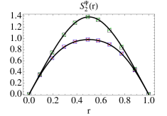
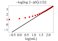
Figure 2: Numerical results for the case $n=2$ on the toric lattice $[0,L]^{2}$ with $L=50$ and lattice spacing $\Delta x=1$. Left. Two-particle states $|\Psi\rangle=|\vec{p}_{1},\vec{p}_{2}\rangle$. Squares are for mass $m=1$ and small momenta, crosses are for mass $m=0.001$ and large momenta. The upper curve is formula (4) for $\Delta S_{2}^{1,1}$, with numerical results for distinct momenta $\vec{p}_{1}=(0,0),\,\vec{p}_{2}=(0.26,0)=(4\pi/L,0)$ (squares) and $\vec{p}_{1}=(2.51,1.26)=(40\pi/L,20\pi/L),\,\vec{p}_{2}=(3.14,0)=(50\pi/L,0)$ (crosses). The lower curve is formula (3) for $\Delta S_{2}^{2}$, with numerical results for equal momenta $\vec{p}_{1}=\vec{p}_{2}=(0.13,0)=(2\pi/L,0)$ (squares) and $\vec{p}_{1}=\vec{p}_{2}=(2.51,1.26)$ (crosses). Right. Approach of $\Delta S_{2}^{1}(1/2)$ to the analytical value $\log 2$ for the one-particle state $|\Psi\rangle=|\vec{p}\rangle$ with $\vec{p}=(0,0)$ as a function of $L$. This shows a linear approach for large $mL$. The solid line is the fit $0.527-1.783\log(mL)$ on the last 8 data points ($mL\in[6.5,10]$).

The qubit interpretation presented earlier suggests that our results need not be restricted to one-dimensional QFT. To test this claim, we performed a numerical evaluation of the quantity $\Delta S_{n}^{\Psi}(r)$ in the harmonic chain and the two-dimensional harmonic lattice. We present some of our results in FIG. 2 and in the supplementary material (SM). We used wave-functional methods in order to represent the state $|\Psi\rangle$. In the finite-volume Klein-Gordon theory, the vacuum wave functional takes the form

$$\langle\varphi|0\rangle\propto\exp\left[-\frac{1}{2}\int_{C\times C}{\rm d}^{d}x\,{\rm d}^{d}y\,K(\vec{x}-\vec{y})\varphi(\vec{x})\varphi(\vec{y})\right]$$ (16)

where $K(\vec{x})=\sum_{\vec{p}}{\rm Vol}_{d}\,(C)^{-1}E_{\vec{p}}\,e^{{\rm i}\vec{p}\cdot\vec{x}}$. Excited state wave functionals are obtained by applying the operator

$$A^{\dagger}(\vec{p})=\frac{\int_{C}{\rm d}^{d}x\,e^{{\rm i}\vec{p}\cdot\vec{x}}\left(E_{\vec{p}}\varphi(\vec{x})-{\rm i}\varpi(\vec{x})\right)}{\sqrt{2E_{\vec{p}}\,{\rm Vol}_{d}\,(C)}},\ [A_{\vec{p}},A^{\dagger}_{\vec{q}}]=\delta_{{\vec{p}},{\vec{q}}},$$ (17)

(where $E_{\vec{p}}=\sqrt{\vec{p}^{2}+m^{2}}$) with the representation of the canonical momentum $\varpi(\vec{x})=-{\rm i}\delta/\delta\varphi(\vec{x})$ satisfying $[\varphi(\vec{x}),\varpi(\vec{y})]={\rm i}\delta(\vec{x}-\vec{y})$. This generates factors which are polynomial functionals of $\varphi(\vec{x})$. The operator $\mathbb{T}(A,B)$ is easily implemented on the space of field configurations. The ratio (13) then becomes a Gaussian average of polynomial functionals of the fields. Discretising space to a finite lattice spacing $\Delta x$ modifies the dispersion relation to $E_{\vec{p}}^{2}=m^{2}+4\sum_{i=1}^{d}\sin^{2}(p_{i}\Delta x/2)/(\Delta x)^{2}$. Numerical results in the one-dimensional case are discussed in more detail in ussoon , where both QFT and non-universal parameter regimes are seen to agree with our predictions, for connected and disconnected regions. We concentrate here on the two-dimensional periodic square lattice on $C=[0,L]^{2}$. We choose a set of subregions $A=[0,\ell]^{2}$ for values of $r=\ell^{2}/L^{2}$ ranging between 0 and 1. In order to establish the validity of the requirements on the correlation length $\xi$ and the De Broglie wavelength $\zeta$, we explore two distinct regimes: that of small $\xi$ but large $\zeta$, and that of small $\zeta$ but large $\xi$, in both cases looking at two-particle states with equal and with distinct rapidities. We find excellent agreement with formulae (4) for $\Delta S_{n}^{1,1}$ and (3) for $\Delta S_{n}^{2}$, respectively, see FIG. 2. Note that the configuration we have chosen is not symmetric: regions $A$ and $B$ have different shapes. Nevertheless, the symmetry $r\mapsto 1-r$ is correctly recovered in the regime of validity of formulae (3) and (4). We have explored other shapes of the region $A$, obtaining similar accuracy, and have analysed regimes where both $\xi$ and $\zeta$ are small, finding even greater accuracy. We have also analysed the breaking of formulae (3) and (4) away from their regime of validity. The approach to the maximum $\log 2$ in the case of a single particle with $r=1/2$ (this maximal value is supported by general arguments ln2 ) is shown in FIG. 2, where the correlation length is varied; we observe an algebraic approach at large $mL$.

For particular choices of the region $A$, it is possible to show analytically the results (3–8) in the massive Klein-Gordon and Majorana models of any higher dimension, by dimensional reduction KG . Consider the slab-like regions $A=[0,\ell]\times C_{\perp}$ in $C=[0,L]\times C_{\perp}$ where $C_{\perp}$ is some $d-1$-dimensional space. From the $d$-dimensional Klein-Gordon fields $\varphi(\vec{x},t)$ and $\varpi(\vec{x},t)$ construct

$$\hat{\varphi}(x_{1},t)=\frac{\int_{C_{\perp}}{\rm d}^{d-1}x_{\perp}\varphi(x_{1},\vec{x}_{\perp},t)}{\sqrt{{\rm Vol}_{d-1}\,(C_{\perp})}}$$ (18)

and similarly for $\hat{\varpi}(x_{1},t)$ in terms of $\varpi(\vec{x},t)$. One observes that $\hat{\varphi}(x,t)$ and $\hat{\varpi}(x,t)$ are canonically normalised one-dimensional Klein-Gordon fields, and that the dimensional reduction map preserves the vacuum KG . It also preserves the many-particle states when all momenta point in the $x_{1}$ direction: with $\vec{p}=(p,0,\ldots,0)$ the expression (17) gives $A^{\dagger}(\vec{p})=\hat{A}^{\dagger}(p)$. Therefore, the quantity ${}_{n}\langle\Psi|\mathbb{T}(\lambda A,\lambda B)|\Psi\rangle_{n}$ in $d$ dimensions, is proportional to ${}_{n}\langle\hat{\Psi}|\mathcal{T}(0)\tilde{\mathcal{T}}(\ell)|\hat{\Psi}\rangle_{n}$ in 1 dimension. The singularity as $\ell\to 0$ is dimension dependent, but in the ratio (13), this cancels out, and there is exact equality. See ussoon for more details. This analysis extends to other quasi-one-dimensional configurations.

Finally, we establish that our results hold beyond free theories. We analyse the quantity $\Delta S_{n}^{\Psi}(r)$ in interacting states of the Bethe ansatz form. Previous analyses exist Vincenzo ; Vincenzo2 , which however concentrated on less universal regimes. In the ferromagnetic Heisenberg chain, two-particle states with respect to the ferromagnetic vacuum have the simple form $\sum_{x,y\in{\mathbb{Z}}}e^{{\rm i}px+{\rm i}qy}S_{{\rm sgn}(x-y)}(p,q)|\uparrow\cdots\downarrow_{x}\cdots\uparrow\cdots\downarrow_{y}\cdots\uparrow\rangle$, where $S_{\epsilon}(p,q)$ is the Bethe ansatz scattering matrix. As in the context of the thermodynamic Bethe ansatz formalism of integrable QFT tba1 ; tba2 , for the purpose of evaluating large-distance quantities these are abstract states representing two-particle asymptotic states, with $S_{\epsilon}(p,q)$ the two-body scattering matrix of the field theory. States of the Bethe ansatz form thus are expected to provide large-distance results of great generality in integrable models. We have analysed such one- and two-particle states, and found that formulae (3) and (4) hold, see the SM. There is no need to fix the momenta via the Bethe ansatz; with equal momenta $S_{n}^{2}(r)$ is indeed reproduced, extending previous results. Bound states of the Heisenberg chains (Bethe strings) have been studied Vincenzo ; these have an intrinsic length scale $\xi$ (inversely proportional to the bounding energy), and one can see that in the regimes discussed above, $S_{n}^{1}(r)$ is indeed reproduced.

Discussion.— It is remarkable that the entanglement of a wide variety of many-body quantum systems admits such a simple and universal “qubit” interpretation. This combines a semiclassical picture of localised particles controlled by correlation lengths and De Broglie wavelengths, with the quantum effect of (in)distinguishability. The applicability of equations (3–8) to higher dimensions is particularly significant, showing that a large amount of geometric information is irrelevant. Their application to QFT is also interesting: QFT locality is formally based on the vanishing of space-like commutation relations, not on particles, yet our results show how quantum entanglement clearly “sees” localised particles. The results hold beyond the QFT regime, as we checked in quantum harmonic lattices and in Bethe ansatz excitations of quantum spin chains. Going beyond integrability, the results are fully expected to hold when no particle production occurs, for instance in QFT one-particle states, and two-particle states below the particle production threshold. In fact, any one- and two-particle excitations of Bethe-ansatz form will have EE described by (3)-(8), such as in spin-preserving quantum chains, integrable or not. The relation (12) also suggests that quasi-particle excitations in extended systems of any dimension can be used to create simple entangled states with controllable entanglement, where the control parameter is the region-to-system volume ratio $r$. It would be interesting to investigate the possible applications of such a result in the area of quantum information.

Acknowledgements:

We are grateful to EPSRC for funding through the standard proposal “Entanglement Measures, Twist Fields, and Partition Functions in Quantum Field Theory” under reference numbers EP/P006108/1 and EP/P006132/1. We would also like to thank Vincenzo Alba for discussions and for bringing reference Vincenzo to our attention.

Appendix A Supplementary Material

Appendix B Rényi Entropy of one- and two-Magnon States in Gapped Quantum Spin Chains

In this section we present a derivation of the nth Rényi entropy for a one-magnon state and the 2nd Rényi entropy of a two-magnon state in a generic gapped quantum spin-$\frac{1}{2}$ chain of length $L$. There is some overlap with calculations presented in the appendices of Vincenzo but the focus is slightly different here. An obvious example would be the XXZ model in the gapped regime but other models can also be included, as long as their excited states can be represented as

$$|\Psi\rangle_{1}=\frac{1}{\sqrt{L}}\sum_{j=1}^{L}e^{ipj}|j\rangle,$$ (19)

and

$$|\Psi\rangle_{2}=\frac{1}{\sqrt{N}}\sum_{j_{1},j_{2}=1}^{L}S_{j_{1}j_{2}}e^{ip_{1}j_{1}+ip_{2}j_{2}}|j_{1}j_{2}\rangle,$$ (20)

where

$$S_{j_{1}j_{2}}=(S_{j_{1}j_{2}}^{*})^{-1}=\left\{\begin{array}[]{cc}e^{i\varphi}&\mathrm{for}\quad j_{1}>j_{2}\\ 1&\mathrm{for}\quad j_{1}<j_{2}\\ 0&\mathrm{for}\quad j_{1}=j_{2}\end{array}\right.$$ (21)

for a two-particle excited state. The states $|j\rangle$ and $|j_{1}j_{2}\rangle$ represent tensor product states where all spins are up, except the spin at position $j$ or the spins at positions $j_{1},j_{2}$, respectively. The normalization $N$ of the two-particle excited state will be discussed below. In our computations we will consider a bi-partition such that

$$\mathrm{spins}\,\,\{1,\ldots,\ell\}\in A\quad\mathrm{and}\quad\mathrm{spins}\,\,\{\ell+1,\ldots,L\}\in B$$ (22)

The choice of the spins is relevant in the computations below as it determines the value of the scattering phases (21). However, it is easy to show that this choice is not essential. That is, the results would be identical in the regions $A$ and $B$ are not simply-connected. Finally we note that we will use the notation

$$r:=\frac{\ell}{L}$$ (23)

to denote the dimensionless ratio of length scales in the problem.

B.1 One-Magnon State

Consider the state (19). The basic states are normalized as $\langle j_{1}|j_{2}\rangle=\delta_{j_{1}j_{2}}$ and therefore the state above has norm 1. We would like to compute the Rényi entropy of region $A$ for the state $|\Psi\rangle$. This computation is actually very simple and the results have been presented for instance in Berko . Let us first compute the reduced density matrix

$$\rho_{A}=\mathrm{Tr}_{B}(|\Psi\rangle_{1}{}_{1}\langle\Psi|).$$ (24)

This is

$$\rho_{A} = \frac{1}{L}\mathrm{Tr}_{B}\left(\sum_{j,k=1}^{L}e^{ip(j-k)}|j\rangle\langle k|\right)$$ (25)

$$= \frac{1}{L}\sum_{j,k\in A}e^{ip(j-k)}|j\rangle\langle k|\mathrm{Tr}_{B}\left(|0\rangle\langle 0|\right)+\frac{1}{L}|0\rangle\langle 0|\sum_{j,k\in B}e^{ip(j-k)}\mathrm{Tr}_{B}\left(|j\rangle\langle k|\right)$$

$$+\frac{1}{L}\sum_{j\in A}e^{ipj}|j\rangle\langle 0|\sum_{k\in B}e^{-ipk}\mathrm{Tr}_{B}\left(|0\rangle\langle k|\right)+\frac{1}{L}\sum_{k\in A}e^{-ipk}|0\rangle\langle k|\sum_{j\in B}e^{ipj}\mathrm{Tr}_{B}\left(|j\rangle\langle 0|\right)$$

$$= \frac{1}{L}\sum_{j,k\in A}e^{ip(j-k)}|j\rangle\langle k|+\frac{L-\ell}{L}|0\rangle\langle 0|,$$

where $|0\rangle$ represents the vacuum state. To compute the Rényi entropy we need to take the $n$-th power of the matrix above and then the trace thereof. When doing so the two contributions do not mix so we can write:

$$\mathrm{Tr}_{A}\rho_{A}^{n}=\mathrm{Tr}_{A}(\frac{1}{L}\sum_{j,k\in A}e^{ip(j-k)}|j\rangle\langle k|)^{n}+\mathrm{Tr}_{A}(\frac{L-\ell}{L}|0\rangle\langle 0|)^{n}$$ (26)

The first term is

$$\mathrm{Tr}_{A}(\frac{1}{L}\sum_{j,k\in A}e^{ip(j-k)}|j\rangle\langle k|)^{n} = \mathrm{Tr}_{A}\left(\frac{1}{L^{n}}\sum_{{k_{1},\ldots,k_{n}\in A}\atop{j_{1},\ldots,j_{n}\in A}}e^{ipj_{1}}|j_{1}\rangle\left[\prod_{i=1}^{n-1}e^{ip(j_{i+1}-k_{i})}\langle k_{i}|j_{i+1}\rangle\right]e^{-ipk_{n}}\langle k_{n}|\right)$$ (27)

$$= \mathrm{Tr}_{A}\left(\frac{1}{L^{n}}\sum_{{k_{1},\ldots,k_{n}\in A}\atop{j_{1},\ldots,j_{n}\in A}}e^{ipj_{1}}|j_{1}\rangle\left[\prod_{i=1}^{n-1}\prod_{i=1}^{n-1}e^{ip(j_{i+1}-k_{i})}\delta_{k_{i}j_{i+1}}\right]e^{-ipk_{n}}\langle k_{n}|\right)$$

$$= \frac{1}{L^{n}}\sum_{{k_{1},\ldots,k_{n}\in A}\atop{j_{1},\ldots,j_{n}\in A}}\delta_{j_{1}k_{n}}\left[\prod_{i=1}^{n-1}\delta_{k_{i}j_{i+1}}\right]=\frac{\ell^{n}}{L^{n}}=r^{n}.$$

The second term is simply

$$\mathrm{Tr}_{A}(\frac{L-\ell}{L}|0\rangle\langle 0|)^{n}=\frac{(L-\ell)^{n}}{L^{n}}=(1-r)^{n}.$$ (28)

Which gives the known formula for the entanglement of a single excitation:

$$S_{n}^{1}(r)=\frac{\log(r^{n}+(1-r)^{n})}{1-n}.$$ (29)

Note that if the ground state is factorizable (as in the XXZ gapped chain) and therefore has zero entropy the result gives us the entanglement of the excited state directly. Note that all functions (29) have a maximum for $r=\frac{1}{2}$

$$S_{n}^{1}(1/2)=\log 2,$$ (30)

including the limits $n\rightarrow 1$ and $n\rightarrow\infty$ (see FIG. 1). The fact that one-particle excitations contribute $\log 2$ to the entanglement entropy was studied in detail in ln2 where it was shown to be case even for a non-integrable spin chain model.

B.2 Two-Magnon State

The effect of the presence of non-trivial interaction can be explored by considering a two-magnon state such as (20).

B.3 State Normalization

We will start by fixing the normalization of the state, $N$. The norm is

$${}_{2}\langle\Psi|\Psi\rangle_{2} = \frac{1}{N}\sum_{{j_{1},j_{2},j_{1}^{\prime}j_{2}^{\prime}=1}}^{L}S_{j_{1}j_{2}}S_{j_{1}^{\prime}j_{2}^{\prime}}^{*}e^{ip_{1}(j_{1}-j_{1}^{\prime})+ip_{2}(j_{2}-j_{2}^{\prime})}\langle j_{1}^{\prime}j_{2}^{\prime}|j_{1}j_{2}\rangle$$ (31)

$$= \frac{1}{N}\sum_{{j_{1},j_{2},j_{1}^{\prime}j_{2}^{\prime}=1}}^{L}S_{j_{1}j_{2}}S_{j_{1}^{\prime}j_{2}^{\prime}}^{*}e^{ip_{1}(j_{1}-j_{1}^{\prime})+ip_{2}(j_{2}-j_{2}^{\prime})}[\delta_{j_{1}j_{1}^{\prime}}\delta_{j_{2}j_{2}^{\prime}}+\delta_{j_{1}j_{2}^{\prime}}\delta_{j_{2}j_{1}^{\prime}}]$$

$$= \frac{1}{N}\sum_{j_{1},j_{2}=1}^{L}\left[1-\delta_{j_{1}j_{2}}+S_{j_{1}j_{2}}S_{j_{2}j_{1}}^{*}e^{ip_{12}j_{12}}\right],$$

where $p_{12}:=p_{1}-p_{2}$ and $j_{12}:=j_{1}-j_{2}$. Using the definition of the $S$-matrix we have that we can rewrite the sum as

$${}_{2}\langle\Psi|\Psi\rangle_{2} = \frac{L(L-1)}{N}+\frac{1}{N}\sum_{j_{1}=2}^{L}\sum_{j_{2}=1}^{j_{1}-1}\left[S_{j_{1}j_{2}}S_{j_{2}j_{1}}^{*}e^{ip_{12}j_{12}}+S_{j_{2}j_{1}}S_{j_{1}j_{2}}^{*}e^{ip_{12}j_{21}}\right]$$ (32)

$$= \frac{L(L-1)}{N}+\frac{1}{N}\sum_{j_{1}=2}^{L}\sum_{j_{2}=1}^{j_{1}-1}\left[e^{i\varphi}e^{ip_{12}j_{12}}+e^{-i\varphi}e^{ip_{12}j_{21}}\right]$$

$$= \frac{L(L-1)}{N}+\frac{1}{N}\sum_{j_{1}=2}^{L}\sum_{j_{2}=1}^{j_{1}-1}\left[2\cos(\varphi+p_{12}j_{12})\right]$$

$$= \frac{L(L-1)}{N}+\frac{1}{N}\frac{(L-1)\cos\varphi-L\cos(\varphi+p_{12})+\cos(\varphi+Lp_{12})}{\cos p_{12}-1}.$$

Thus,

$$N={L(L-1)}+\frac{(L-1)\cos\varphi-L\cos(\varphi+p_{12})+\cos(\varphi+Lp_{12})}{\cos p_{12}-1}.$$ (33)

This same formula was given also in one of the appendices in Vincenzo . Clearly, for $L$ large and $p_{12}\neq 0$, the second contribution is sub-leading so that

$$N\approx L^{2}\quad\mathrm{for}\quad L\quad\mathrm{large}.$$ (34)

B.4 Computation of the Reduced Density Matrix

We now need to proceed as for the first example. First we compute the reduce density matrix

$$\rho_{A}=\frac{1}{N}\mathrm{Tr}_{B}\left(\sum_{j_{1},j_{2},k_{1},k_{2}=1}^{L}S_{j_{1}j_{2}}S_{k_{1}k_{2}}^{*}e^{ip_{1}(j_{1}-k_{1})+ip_{2}(j_{2}-k_{2})}|j_{1}j_{2}\rangle\langle k_{1}k_{2}|\right).$$ (35)

The only non-vanishing contributions to this trace come from those terms were either all indices are in $A$, all are in $B$ or two indices are in $A$ and two indices are in $B$. This gives the following six contributions:

$$\rho_{A} = \frac{1}{N}\sum_{j_{1},j_{2},k_{1},k_{2}\in A}S_{j_{1}j_{2}}S_{k_{1}k_{2}}^{*}e^{ip_{1}(j_{1}-k_{1})+ip_{2}(j_{2}-k_{2})}|j_{1}j_{2}\rangle\langle k_{1}k_{2}|\,\mathrm{Tr}_{B}(|0\rangle\langle 0|)$$ (36)

$$+ \frac{1}{N}\sum_{j_{1},j_{2},k_{1},k_{2}\in B}S_{j_{1}j_{2}}S_{k_{1}k_{2}}^{*}e^{ip_{1}(j_{1}-k_{1})+ip_{2}(j_{2}-k_{2})}|0\rangle\langle 0|\,\mathrm{Tr}_{B}\left(|j_{1}j_{2}\rangle\langle k_{1}k_{2}|\right)$$

$$+ \frac{1}{N}\sum_{j_{1},k_{1}\in A,j_{2},k_{2}\in B}S_{j_{1}j_{2}}S_{k_{1}k_{2}}^{*}e^{ip_{1}(j_{1}-k_{1})+ip_{2}(j_{2}-k_{2})}|j_{1}\rangle\langle k_{1}|\,\mathrm{Tr}_{B}\left(|j_{2}\rangle\langle k_{2}|\right)$$

$$+ \frac{1}{N}\sum_{j_{1},k_{2}\in A,j_{2},k_{1}\in B}S_{j_{1}j_{2}}S_{k_{1}k_{2}}^{*}e^{ip_{1}(j_{1}-k_{1})+ip_{2}(j_{2}-k_{2})}|j_{1}\rangle\langle k_{2}|\,\mathrm{Tr}_{B}\left(|j_{2}\rangle\langle k_{1}|\right)$$

$$+ \frac{1}{N}\sum_{j_{2},k_{1}\in A,j_{1},k_{2}\in B}S_{j_{1}j_{2}}S_{k_{1}k_{2}}^{*}e^{ip_{1}(j_{1}-k_{1})+ip_{2}(j_{2}-k_{2})}|j_{2}\rangle\langle k_{1}|\,\mathrm{Tr}_{B}\left(|j_{1}\rangle\langle k_{2}|\right)$$

$$+ \frac{1}{N}\sum_{j_{2},k_{2}\in A,j_{1},k_{1}\in B}S_{j_{1}j_{2}}S_{k_{1}k_{2}}^{*}e^{ip_{1}(j_{1}-k_{1})+ip_{2}(j_{2}-k_{2})}|j_{2}\rangle\langle k_{2}|\,\mathrm{Tr}_{B}\left(|j_{1}\rangle\langle k_{1}|\right)$$

Noting that

$$\mathrm{Tr}_{B}(|j_{1}\rangle\langle k_{1}|)=\delta_{j_{1}k_{1}},\quad\mathrm{Tr}_{B}(|j_{1}j_{2}\rangle\langle k_{1}k_{2}|)=\delta_{j_{1}k_{1}}\delta_{j_{2}k_{2}}+\delta_{j_{1}k_{2}}\delta_{j_{2}k_{1}},$$ (37)

and grouping all four last terms together by relabelling the summation indices, the reduced density matrix simplifies to:

$$\rho_{A} = \frac{1}{N}\sum_{j_{1},j_{2},k_{1},k_{2}\in A}S_{j_{1}j_{2}}S_{k_{1}k_{2}}^{*}e^{ip_{1}(j_{1}-k_{1})+ip_{2}(j_{2}-k_{2})}|j_{1}j_{2}\rangle\langle k_{1}k_{2}|$$ (38)

$$+ \frac{1}{N}\sum_{j_{1},j_{2},k_{1},k_{2}\in B}S_{j_{1}j_{2}}S_{k_{1}k_{2}}^{*}e^{ip_{1}(j_{1}-k_{1})+ip_{2}(j_{2}-k_{2})}|0\rangle\langle 0|\,(\delta_{j_{1}k_{1}}\delta_{j_{2}k_{2}}+\delta_{j_{1}k_{2}}\delta_{j_{2}k_{1}})$$

$$+ \frac{1}{N}\sum_{j_{1},k_{1}\in A,j_{2},k_{2}\in B}(S_{j_{1}j_{2}}S_{k_{1}k_{2}}^{*}e^{ip_{1}(j_{1}-k_{1})+ip_{2}(j_{2}-k_{2})}+S_{j_{1}j_{2}}S_{k_{2}k_{1}}^{*}e^{ip_{1}(j_{1}-k_{2})+ip_{2}(j_{2}-k_{1})}$$

$$+S_{j_{2}j_{1}}S_{k_{1}k_{2}}^{*}e^{ip_{1}(j_{2}-k_{1})+ip_{2}(j_{1}-k_{2})}+S_{j_{2}j_{1}}S_{k_{2}k_{1}}^{*}e^{ip_{1}(j_{2}-k_{2})+ip_{2}(j_{1}-k_{1})})|j_{1}\rangle\langle k_{1}|\,\delta_{j_{2}k_{2}}.$$

In the last sum all $S$-matrices have one index in region $A$ and the other in region $B$ so we can use the $S$-matrix definition to simplify the expression. Applying the $\delta$-functions we can write,

$$\rho_{A}=\frac{1}{N}(\rho_{A}^{(1)}+\rho_{A}^{(2)}+\rho_{A}^{(3)}),$$ (39)

where we introduced the matrices

$$\rho_{A}^{(1)} = \sum_{j_{1},j_{2},k_{1},k_{2}\in A}S_{j_{1}j_{2}}S_{k_{1}k_{2}}^{*}e^{ip_{1}(j_{1}-k_{1})+ip_{2}(j_{2}-k_{2})}|j_{1}j_{2}\rangle\langle k_{1}k_{2}|$$ (40)

$$\rho_{A}^{(2)} = \sum_{j_{1},j_{2}\in B}(S_{j_{1}j_{2}}S_{j_{1}j_{2}}^{*}+S_{j_{1}j_{2}}S_{j_{2}j_{1}}^{*}e^{ip_{12}j_{12}})|0\rangle\langle 0|$$ (41)

$$\rho_{A}^{(3)} = \sum_{{{j_{2}\in B}}\atop{j_{1},k_{1}\in A}}[e^{ip_{1}(j_{1}-k_{1})}+e^{ip_{2}(j_{1}-k_{1})}+e^{ip_{1}j_{12}+ip_{2}(j_{2}-k_{1})-i\varphi}+e^{ip_{2}j_{12}+ip_{1}(j_{2}-k_{1})+i\varphi}]|j_{1}\rangle\langle k_{1}|.$$ (42)

B.5 2nd Rényi Entropy

To compute the second Rényi entropy we must compute the square of the expression above and then take the trace over subspace $A$. It is easy to show that the only contributions to the trace will come from the squaring each of the three terms above separately, so we can ignore cross-terms that will vanish under the trace.

For the first term squaring and taking the trace gives

$$\mathrm{Tr}_{A}((\rho_{A}^{(1)})^{2}) = \sum_{{j^{\prime}_{1},j^{\prime}_{2},k^{\prime}_{1},k^{\prime}_{2}\in A}\atop{j_{1},j_{2},k_{1},k_{2}\in A}}S_{j_{1}j_{2}}S_{k_{1}k_{2}}^{*}S_{j^{\prime}_{1}j^{\prime}_{2}}S_{k^{\prime}_{1}k^{\prime}_{2}}^{*}e^{ip_{1}(j_{1}+j^{\prime}_{1}-k_{1}-k^{\prime}_{1})+ip_{2}(j_{2}+j^{\prime}_{2}-k_{2}-k_{2}^{\prime})}$$ (43)

$$\qquad\qquad\times(\delta_{j_{1}k^{\prime}_{1}}\delta_{j_{2}k^{\prime}_{2}}+\delta_{j_{1}k^{\prime}_{2}}\delta_{j_{2}k^{\prime}_{1}})(\delta_{k_{1}j^{\prime}_{1}}\delta_{k_{2}j^{\prime}_{2}}+\delta_{k_{1}j^{\prime}_{2}}\delta_{k_{2}j^{\prime}_{1}})$$

$$=\sum_{{j_{1},j_{2},k_{1},k_{2}\in A}}S_{j_{1}j_{2}}S_{k_{1}k_{2}}^{*}e^{ip_{1}(j_{1}-k_{1})+ip_{2}(j_{2}-k_{2})}$$

$$\times\left(S_{k_{1}k_{2}}S_{j_{1}j_{2}}^{*}e^{ip_{1}(k_{1}-j_{1})+ip_{2}(k_{2}-j_{2})}+S_{k_{2}k_{1}}S_{j_{1}j_{2}}^{*}e^{ip_{1}(k_{2}-j_{1})+ip_{2}(k_{1}-j_{2})}\right.$$

$$\left.+S_{k_{1}k_{2}}S_{j_{2}j_{1}}^{*}e^{ip_{1}(k_{1}-j_{2})+ip_{2}(k_{2}-j_{1})}+S_{k_{2}k_{1}}S_{j_{2}j_{1}}^{*}e^{ip_{1}(k_{2}-j_{2})+ip_{2}(k_{1}-j_{1})}\right),$$

where, in the first equality, we used the fact that

$$\mathrm{Tr}_{A}(|j_{1}j_{2}\rangle\langle k_{1}k_{2}|j^{\prime}_{1}j_{2}^{\prime}\rangle\langle k^{\prime}_{1}k^{\prime}_{2}|)=(\delta_{j_{1}k^{\prime}_{1}}\delta_{j_{2}k^{\prime}_{2}}+\delta_{j_{1}k^{\prime}_{2}}\delta_{j_{2}k^{\prime}_{1}})(\delta_{k_{1}j^{\prime}_{1}}\delta_{k_{2}j^{\prime}_{2}}+\delta_{k_{1}j^{\prime}_{2}}\delta_{k_{2}j^{\prime}_{1}}).$$ (44)

Employing the explicit form of the $S$-matrices, the expression can be greatly simplified and factorizes as

$$\mathrm{Tr}_{A}((\rho_{A}^{(1)})^{2})=\left[\sum_{{k_{1}k_{2}\in A}}\left(1-\delta_{k_{1}k_{2}}+S_{k_{1}k_{2}}^{*}S_{k_{2}k_{1}}e^{ip_{12}k_{21}}\right)\right]^{2}.$$ (45)

The sum over the $S$-matrices can be computed by for instance splitting it into the contribution with $k_{1}>k_{2}$ and the contribution with $k_{1}<k_{2}$. For example

$$\sum_{{k_{1}k_{2}\in A}}S_{k_{1}k_{2}}^{*}S_{k_{2}k_{1}}e^{ip_{12}k_{21}} = \sum_{{k_{1}k_{2}\in A}}S_{k_{1}k_{2}}^{*}S_{k_{2}k_{1}}e^{ip_{12}k_{21}}$$ (46)

$$= \sum_{k_{1}=1}^{\ell}\sum_{k_{2}=1}^{k_{1}-1}(S_{k_{1}k_{2}}^{*}S_{k_{2}k_{1}}e^{ip_{12}k_{21}}+S_{k_{2}k_{1}}^{*}S_{k_{1}k_{2}}e^{ip_{12}k_{12}})$$

$$= \sum_{k_{1}=1}^{\ell}\sum_{k_{2}=1}^{k_{1}-1}(e^{-i\varphi}e^{ip_{12}k_{21}}+e^{i\varphi}e^{ip_{12}k_{12}})$$

$$= 2\sum_{k_{1}=1}^{\ell}\sum_{k_{2}=1}^{k_{1}-1}\cos(\varphi+p_{12}k_{12})$$

$$= \frac{(\ell-1)\cos\varphi-\ell\cos(\varphi+p_{12})+\cos(\varphi+\ell p_{12})}{\cos p_{12}-1}.$$

Thus, the full contribution to the 2nd Rényi entropy (up to normalization of the state) is given by

$$\mathrm{Tr}_{A}((\rho_{A}^{(1)})^{2})=\left[\ell(\ell-1)+\frac{(\ell-1)\cos\varphi-\ell\cos(\varphi+p_{12})+\cos(\varphi+\ell p_{12})}{\cos p_{12}-1}\right]^{2}$$ (47)

Clearly, for $L,\ell$ large and $p_{12}\neq 0$ and considering (34) the leading contribution to the entanglement entropy is

$$\frac{1}{N^{2}}\mathrm{Tr}_{A}((\rho_{A}^{(1)})^{2})\approx r^{4}.$$ (48)

It is easy to show that the contribution to the 2nd Rényi entropy of the the second term in (39) is identical to the above, with the replacement $\ell\rightarrow L-\ell$. That is,

$$\mathrm{Tr}_{A}((\rho_{A}^{(2)})^{2})=$$

$$\left[(L-\ell)(L-\ell-1)+\frac{(L-\ell-1)\cos\varphi-(L-\ell)\cos(\varphi+p_{12})+\cos(\varphi+(L-\ell)p_{12})}{\cos p_{12}-1}\right]^{2}.$$ (49)

for $L,\ell$ large and $p_{12}\neq 0$ the leading contribution is

$$\frac{1}{N^{2}}\mathrm{Tr}_{A}((\rho_{A}^{(2)})^{2})\approx(1-r)^{4}.$$ (50)

Let us now consider then the third term $\rho_{A}^{(3)}$. After computing the square and then the trace over subspace $A$ and noting that

$$\mathrm{Tr}_{A}(|j_{1}\rangle\langle k_{1}|j^{\prime}_{1}\rangle\langle k^{\prime}_{1}|)=\delta_{j_{1}k^{\prime}_{1}}\delta_{j^{\prime}_{1}k_{1}},$$ (51)

we find

$$\mathrm{Tr}_{A}((\rho_{A}^{(3)})^{2})=\sum_{{j_{2},j^{\prime}_{2}\in B}\atop{j_{1},k_{1}\in A}}(e^{ip_{1}(j_{1}-k_{1})}+e^{ip_{2}(j_{1}-k_{1})}+e^{-i\varphi}e^{ip_{1}j_{12}+ip_{2}(j_{2}-k_{1})}+e^{i\varphi}e^{ip_{2}j_{12}+ip_{1}(j_{2}-k_{1})})$$

$$\qquad\quad\times(e^{ip_{1}(k_{1}-j_{1})}+e^{ip_{2}(k_{1}-j_{1})}+e^{-i\varphi}e^{ip_{1}(k_{1}-j^{\prime}_{2})+ip_{2}(j^{\prime}_{2}-j_{1})}+e^{i\varphi}e^{ip_{2}(k_{1}-j^{\prime}_{2})+ip_{1}(j^{\prime}_{2}-j_{1})}))$$ (52)

Expanding the product and simplifying we end up with the sum

$$\mathrm{Tr}_{A}((\rho_{A}^{(3)})^{2}) = \sum_{{j_{2},j^{\prime}_{2}\in B}\atop{j_{1},k_{1}\in A}}\left[2+2\cos(p_{12}(j_{1}-k_{1}))+2\cos(\varphi+p_{12}(j^{\prime}_{2}-j_{1}))\right.$$ (53)

$$\left.+2\cos(\varphi+p_{12}(j^{\prime}_{2}-k_{1}))+2\cos(\varphi+p_{12}j_{21})+2\cos(\varphi+p_{12}(j_{2}-k_{1}))\right.$$

$$\left.+2\cos(2\varphi+p_{12}(j^{\prime}_{2}+j_{2}-j_{1}-k_{1}))+2\cos(p_{12}(j_{2}-j^{\prime}_{2}))\right]$$

This is equal to

$$\mathrm{Tr}_{A}((\rho_{A}^{(3)})^{2}) = 2\ell^{2}(L-\ell)^{2}+2(L-\ell)^{2}\frac{\cos(\ell p_{12})-1}{\cos p_{12}-1}+2\ell^{2}\frac{\cos(L-\ell)p_{12}-1}{\cos p_{12}-1}.$$ (54)

$$+2\frac{\cos(2\varphi+Lp_{12})\sin^{2}\frac{\ell p_{12}}{2}\sin^{2}\frac{(L-\ell)p_{12}}{2}}{\sin^{4}\frac{p_{12}}{2}}$$

$$+8\ell(L-\ell)\frac{\cos(\varphi+\frac{Lp_{12}}{2})\sin\frac{\ell p_{12}}{2}\sin\frac{p_{12}(L-\ell)}{2}}{\sin^{2}\frac{p_{12}}{2}}$$

For $\ell,L$ large and $p_{12}\neq 0$ the first term in the sum is leading so the leading contribution to the Rényi entropy is

$$\frac{1}{N^{2}}\mathrm{Tr}_{A}((\rho_{A}^{(3)})^{2})\approx 2r^{2}(1-r)^{2}.$$ (55)

Putting the contributions (48), (50) and (55) together we find that the 2nd Rényi entropy of a two-magnon state for large volume and region size is, as expected.

$$S_{2}^{1,1}(r)=-2\log(r^{2}+(1-r)^{2})=2S_{2}^{1}(r),$$ (56)

that is, as expected, twice the entropy of a single excitation. Crucially, for large volume, the result is independent of the scattering matrix.

B.6 Equal Momenta

Although in many cases (such as the XXZ chain) the momenta of the magnons is required to be distinct, it is possible to consider spin chains with bosonic statistics, so that $p_{12}=0$ is allowed. In such cases the formulae of the previous section can still be used, but the terms involving trigonometric functions, which were negligible at large volume, are no-longer so. Indeed, they now become of the same order as the leading terms and it is a simple calculation to show that:

$$N=L(L-1)(1+\cos\varphi),$$ (57)

and

$$\lim_{p_{12}\rightarrow 0}\mathrm{Tr}_{A}((\rho_{A}^{(1)})^{2})=\ell^{2}(\ell-1)^{2}(1+\cos\varphi)^{2},$$ (58)

$$\lim_{p_{12}\rightarrow 0}\mathrm{Tr}_{A}((\rho_{A}^{(2)})^{2})=(L-\ell)^{2}(L-\ell-1)^{2}(1+\cos\varphi)^{2},$$ (59)

$$\lim_{p_{12}\rightarrow 0}\mathrm{Tr}_{A}((\rho_{A}^{(3)})^{2})=4\ell^{2}(L-\ell)^{2}(1+\cos\varphi)^{2}.$$ (60)

Putting these results together, we have that the entanglement entropy is independent of the interaction and this is irrespective of whether or not volume is large. For large volume we find that

$$S_{2}^{2}(r)=-\log(r^{4}+4r^{2}(1-r)^{2}+(1-r)^{4}),$$ (61)

which is different from the expression for distinct momenta of the previous section. The expression agrees with our findings for the free massive boson QFT and the harmonic chain, showing that also for discrete systems the entanglement entropy encodes information about the fermionic/bosonic nature of the quasi-particles. From (58)-(60) it is possible to show the the next to leading order correction for equal momenta is:

$$S_{2}^{2}(r)=-\log(r^{4}+4r^{2}(1-r)^{2}+(1-r)^{4})+\frac{1}{L}\left[1-2\frac{r^{3}+(1-r)^{3}}{r^{4}+4r^{2}(1-r)^{2}+(1-r)^{4}}\right]+O(L^{-2})$$ (62)

In particular at $r=\frac{1}{2}$ were entanglement is maximal ln2 this gives the next-to-leading order correction

$$S_{2}^{2}({1}/{2})=\log\frac{8}{3}+\frac{1}{3L}+O(L^{-2})$$ (63)

It would be interesting to derive such higher order corrections from a QFT computation. A discussion of finize-size corrections to the von Neumann entropy of different kinds of excitations in the XXZ spin-$\frac{1}{2}$ chain was also provided in several of the appendices of Vincenzo .

Appendix C Large Volume Corrections to the 2nd Rényi Entropy in the Harmonic Chain

In this paper we have not presented numerical results for the one-dimensional harmonic chain, whose scaling limit is described by a real massive free boson. Our focus has been on higher dimensions as we intent to discuss the one-dimensional case in much detail in a future work ussoon . However, it is interesting to present here some data regarding the next-to-leading order corrections to the maximal entanglement of an excitation, as they display similar features as in two dimensions (see FIG. 2).

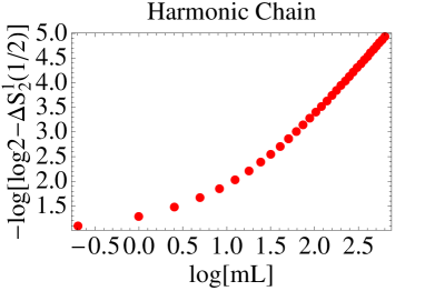
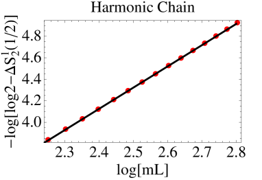
Figure 3: Left. The figure shows the approach to the value $\log 2$ of the 2nd Rényi entropy of a single excitation in a 1D harmonic chain. For large enough volume $mL$ we see linear behaviour with positive slope, meaning that the leading correction is of the form $\beta/L^{\alpha}$ for some $\beta$ and $\alpha$. Right. The figure shows a selection of the points on the first figure which are well fitted by the linear fit $-0.613+1.974\log(mL)$ also shown. The fit changes slightly depending on which points are selected. The behaviour strongly suggests (negative) finite-size corrections of order $1/(mL)^{2}$.

An interesting feature of the results above is that the leading corrections to saturation of the entanglement is of order $1/(mL)^{2}$. From form factor calculations in QFT one would expect a leading correction of order $1/(mL)$ ussoon and it would be interesting to investigate whether or not this correction is also vanishing in QFT. The behaviour above is very similar to what we have found for the harmonic lattice. In that case our data are a bit more limited as we do not have access to extremely large surfaces but, as seen in FIG. 2 they also point towards a $1/L^{\alpha}$ with $\alpha>1$ negative correction to the maximal entanglement of a one-particle state.

References

• (1) C. H. Bennett, H. J. Bernstein, S. Popescu, and B. Schumacher, Concentrating partial entanglement by local operations, Phys. Rev. A53, 2046–2052 (1996).
• (2) G. Vidal and R. F. Werner, Computable measure of entanglement, Phys. Rev. A65, 032314 (2002).
• (3) K. Życzkowski, P. Horodecki, A. Sanpera, and M. Lewenstein, Volume of the set of separable states, Phys. Rev. A58, 883–892 (1998).
• (4) M. B. Plenio, Logarithmic Negativity: A full entanglement monotone that is not convex, Phys. Rev. Lett. 95, 090503 (2005).
• (5) M. B. Plenio, Erratum: logarithmic negativity: a full entanglement monotone that is not convex, Phys. Rev. Lett. 95, 119902 (2005).
• (6) K. Audenaert, J. Eisert, M. B. Plenio, and R. F. Werner, Entanglement properties of the harmonic chain, Phys. Rev. A66, 042327 (2002).
• (7) J. Eisert, Entanglement in quantum information theory (PhD Thesis), quant-ph/0610253 (2006).
• (8) L. Amico, R. Fazio, A. Osterloh, and V. Vedral, Entanglement in many-body systems, Rev. Mod. Phys. 80, 517–576 (2008).
• (9) P. Calabrese, J. Cardy, and B. Doyon (ed), Entanglement entropy in extended quantum systems, J. Phys. A42, 500301 (2009).
• (10) J. Eisert, M. Cramer, and M. B. Plenio, Colloquium: Area laws for the entanglement entropy, Rev. Mod. Phys. 82, 277–306 (2010).
• (11) R. Islam, R. Ma, P. M. Preiss, M. E. Tai, A. Lukin, M. Rispoli, and M. Greiner, Measuring entanglement entropy in a quantum many-body system, Nature 528, 77–83 (2015).
• (12) A. M. Kaufman, M. E. Tai, A. Lukin, M. Rispoli, R. Schittko, P. M. Preiss, and M. Greiner, Quantum thermalization through entanglement in an isolated many-body system, Science 353, 794–800 (2016).
• (13) C. J. Callan and F. Wilczek, On geometric entropy, Phys. Lett. B333, 55–61 (1994).
• (14) C. Holzhey, F. Larsen, and F. Wilczek, Geometric and renormalized entropy in conformal field theory, Nucl. Phys. B424, 443–467 (1994).
• (15) G. Vidal, J. I. Latorre, E. Rico, and A. Kitaev, Entanglement in quantum critical phenomena, Phys. Rev. Lett. 90, 227902 (2003).
• (16) J. I. Latorre, E. Rico, and G. Vidal, Ground state entanglement in quantum spin chains, Quant. Inf. Comput. 4, 48–92 (2004).
• (17) P. Calabrese and J. L. Cardy, Entanglement entropy and quantum field theory, J. Stat. Mech. 0406, P002 (2004).
• (18) P. Calabrese and J. L. Cardy, Evolution of entanglement entropy in one-dimensional systems, J. Stat. Mech. 0504, P010 (2005).
• (19) P. Calabrese, J. Cardy, and E. Tonni, Entanglement entropy of two disjoint intervals in conformal field theory, J. Stat. Mech. 0911, P11001 (2009).
• (20) P. Calabrese, J. Cardy, and E. Tonni, Entanglement negativity in quantum field theory, Phys. Rev. Lett. 109, 130502 (2012).
• (21) P. Calabrese, J. Cardy, and E. Tonni, Entanglement negativity in extended systems: a field theoretical approach, J. Stat. Mech. 1302, P02008 (2013).
• (22) D. Bianchini, O. Castro-Alvaredo, B. Doyon, E. Levi, and F. Ravanini, Entanglement entropy of non-unitary conformal field theory, J.Phys. A48, 04FT01 (2015).
• (23) J. L. Cardy, O. A. Castro-Alvaredo, and B. Doyon, Form factors of branch-point twist fields in quantum integrable models and entanglement entropy, J. Stat. Phys. 130, 129–168 (2008).
• (24) B. Doyon, Bi-partite entanglement entropy in massive two-dimensional quantum field theory, Phys. Rev. Lett. 102, 031602 (2009).
• (25) O. Blondeau-Fournier, O.A. Castro-Alvaredo, and B. Doyon, Universal scaling of the logarithmic negativity in massive quantum field theory, J. Phys. A49(12), 125401 (2016).
• (26) R. V. Jensen and R. Shankar, Statistical behavior in deterministic quantum systems with few degrees of freedom, Phys. Rev. Lett. 54, 1879–1882 (1985).
• (27) J. M. Deutsch, Quantum statistical mechanics in a closed system, Phys. Rev. A43, 2046–2049 (1991).
• (28) M. Srednicki, Chaos and quantum thermalization, Phys. Rev. E 50, 888–901 (1994).
• (29) H. Tasaki, From quantum dynamics to the canonical distribution: general picture and a rigorous example, Phys. Rev. Lett. 80, 1373–1376 (1998).
• (30) M. Rigol, V. Dunjko, and M. Olshanii, Thermalization and its mechanism for generic isolated quantum systems, Nature 452, 854–858 (2008).
• (31) F. C. Alcaraz, M. I. Berganza, and G. Sierra, Entanglement of low-energy excitations in conformal field theory, Phys. Rev. Lett. 106, 201601 (2011).
• (32) M. I. Berganza, F. C. Alcaraz, and G. Sierra, Entanglement of excited states in critical spin chains, J. Stat. Mech. 1201, P01016 (2012).
• (33) J. Mölter, T. Barthel, U. Schollwöck, and V. Alba, Bound states and entanglement in the excited states of quantum spin chains, J. Stat. Mech. 2014(10), P10029 (2014).
• (34) I. Pizorn, Universality in entanglement of quasiparticle excitations, arXiv:1202.3336 (2012).
• (35) M. Storms and R. R. P. Singh, Entanglement in ground and excited states of gapped free-fermion systems and their relationship with Fermi surface and thermodynamic equilibrium properties, Phys. Rev. E89, 012125 (2014).
• (36) R. Berkovits, Two-particle excited states entanglement entropy in a one-dimensional ring, Phys. Rev. B87, 075141 (2013).
• (37) V. Alba, M. Fagotti, and P. Calabrese, Entanglement entropy of excited states, J. Stat. Mech 2009(10), P10020 (2009).
• (38) B. Doyon, A. Lucas, K. Schalm, and M. J. Bhaseen, Non-equilibrium steady states in the Klein-Gordon theory, J. Phys. A48(9), 095002 (2015).
• (39) A. Zamolodchikov, Thermodynamic Bethe ansatz in relativistic models. Scaling three state Potts and Lee-Yang models, Nucl. Phys. B342, 695–720 (1990).
• (40) T. R. Klassen and E. Melzer, The Thermodynamics of purely elastic scattering theories and conformal perturbation theory, Nucl. Phys. B350, 635–689 (1991).
• (41) R. Eden, P. Landshoff, D. Olive, and J. C. Polkinghorne, The analytic S-matrix, Cambridge University Press (1966).
• (42) M. Peskin and D. Schröder, An introduction to quantum field theory, CRC Press (1995).
• (43) J. Eisert and M. Cramer, Single-copy entanglement in critical quantum spin chains, Phys. Rev. A 72, 042112 (2005).
• (44) I. Peschel and J. Zhao, On single-copy entanglement, J. Stat. Mech. 2005(11), P11002 (2005).
• (45) A. Dimic and B. Dakic, Single-copy entanglement detection, Nature Quantum Information 1(4), 11 (2018).
• (46) M. Karowski and P. Weisz, Exact S matrices and form-factors in (1+1)-dimensional field theoretic models with soliton behavior, Nucl. Phys. B139, 455–476 (1978).
• (47) F. Smirnov, Form factors in completely integrable models of quantum field theory, Adv. Series in Math. Phys. 14, World Scientific, Singapore (1992).
• (48) B. Pozsgay and G. Takacs, Form-factors in finite volume I: form-factor bootstrap and truncated conformal space, Nucl. Phys. B788, 167–208 (2008).
• (49) B. Pozsgay and G. Takacs, Form factors in finite volume. II. Disconnected terms and finite temperature correlators, Nucl. Phys. B788, 209–251 (2008).
• (50) O.A. Castro-Alvaredo, C. De Fazio, B. Doyon, and I.M. Szécsényi, Entanglement content of quantum particle excitations I. Free field theory, work in progress.