Correlation energies for many-electron atoms with explicitly correlated Slater functions

Abstract

In this work we propose a novel composite method for accurate calculation of the energies of many-electron atoms. The dominant contribution to the energy (pair energies) are calculated by using explicitly correlated factorisable coupled cluster theory. Instead of the usual Gaussian-type geminals for the expansion of the pair functions, we employ two-electron Hylleraas basis set. This eliminates the need for massive optimisation of nonlinear parameters and the required three-electron integrals can now be calculated relatively easily. The remaining contributions to the energy are calculated within the algebraic approximation by using large one-electron basis sets composed of Slater-type orbitals. The method is tested for the beryllium atom where the accuracy better than $1\,$cm^-1 is obtained. We discuss in details possible sources of the error and estimate the uncertainty in each energy component. Finally, we consider possible strategies to improve the accuracy of the method by one to two orders of magnitude. The most important advantage of the method is that is does not suffer from an exponential growth of the computational costs with increasing number of electrons in the system and thus can be applied to heavier atoms preserving a similar level of accuracy.

I Introduction

Atomic spectroscopy remains an important and active field of modern physics. Many theoretical and experimental works concentrated on different aspects of atomic spectra touch upon very fundamentals of the present scientific knowledge. Search for time-reversal symmetry violations roberts15 , time-dependence of fundamental physical constants rosenband08 ; hunt14 ; godun14 , various empirical tests of the Standard Model and quantum electrodynamics eikema97 ; korobov01 ; pachucki06 ; odom06 ; gabrielse07 are only a handful of prominent examples. Therefore, the need for development of new accurate theoretical tools to predict the atomic spectra (and other relevant quantities) is easy to recognise.

If we restrict ourselves to light atoms, the most accurate theoretical results to date have been obtained with methods where all inter-particle distances are explicitly incorporated into the trial wavefunction. This includes basis sets of Hylleraas-type functions hylleraas29a ; hylleraas29b ; drake94 ; puchalski06 , explicitly-correlated Gaussians (ECG) szalewicz10 ; mitroy13 , Hylleraas-CI expansions sims71 ; sims07 ; king93 , and Slater geminals thakkar77 ; frolov95 ; korobov02 ; puchalski10 . The common problem among these methods, however, is the exponential scaling of the computational costs with the number of particles in the system. Applications to systems larger than, say, five particles are thus scarce and much less accurate.

A different approach to the electronic structure is offered by the coupled clusters (CC) theory bartlett07 . Since the total CC wavefunction is parametrised in terms of a cluster operator which can be truncated in a systematic way, the exponential increase of the computational costs is avoided. The most popular implementation of the CC theory relies on the algebraic approximation, i.e. expansion in a set of one-electron orbitals. Unfortunately, this leads to a relatively slow convergence of the results towards the complete basis set limit hill85 - a manifestation of the Kato’s electron-electron cusp condition kato57 .

One possible remedy to this problem is to abandon the algebraic approximation entirely. To this end, various authors showed that a basis-set independent CC theory can be formulated in terms of the so-called pair functions byron66 ; pan70 ; pan72 ; chalas77 ; szalewicz79 ; szalewicz82 ; szalewicz83a ; szalewicz83b ; szalewicz84a ; szalewicz84b ; adamowicz77 ; adamowicz78a ; adamowicz78b . The pair functions are two-electron objects and thus can be expanded in a basis set which overtly includes all coordinates of the given electron pair. This idea gave rise to the explicitly correlated CC theory.

One of the most difficult obstacles preventing straightforward application of this method is the presence of many-electron integrals. In the modern R12/F12 theory hattig12 ; kong12 ; tenno12 this difficulty is avoided by proper insertions of the resolution of identity (RI) approximation. A different idea has been proposed by Szalewicz and collaborators szalewicz82 ; szalewicz83a ; szalewicz83b who imposed the strong-orthogonality requirement for the pair functions only in the complete basis set limit. This led to a family of weak-orthogonality (WO) functionals. At the second-order Møller-Plesset (MP2) level of theory bartlett07 , for example, this eliminates all four-electron integrals from the working equations, leaving only the relatively simple three-electron ones szalewicz82 ; szalewicz83a .

The WO functionals are typically combined with the Gaussian-type geminals (GTG) for expansion of the CC pair functions. The main advantage of such approach is that the resulting three-electron integrals can be evaluated analytically in a closed form. The remaining inconvenience of the WO theory is the need for optimisation of GTG nonlinear parameters. Despite a considerable effort it seems that this problem has not been satisfactorily resolved thus far. Massive nonlinear optimisations can take months or even years of computer time to converge to a satisfactory result.

With that said, for one-centre systems one can entertain an idea of using the Hylleraas basis set of the form

$$(4\pi)^{-1}r_{1}^{u}\,r_{2}^{v}\,r_{12}^{t}\,\exp(-a_{i}\,r_{1}-a_{j}\,r_{2}),$$ (1)

where $a_{i},a_{j}>0$, and $u$, $v$, $t$ are non-negative integers, for the expansion of the CC pair functions. As explained further in the text, the most important advantage of this basis set is that instead of hundreds or thousands of nonlinear parameters per electron pair one has only a handful of them. Moreover, the basis set (1) can be systematically extended so that the basis set limits and the corresponding errors bars are easier to estimate.

The basis set (1) has not found a significant use in CC theory thus far because of the resulting three-electron integrals. However, in the past two decades a considerable progress has been achieved in attempts to evaluate them analytically and/or recursively. This started with the seminal paper of Fromm and Hill fromm87 who solved the simplest three-electron integral with inverse powers of all interparticle distances. Despite this success and subsequent works remiddi91 ; harris97 the analytic formulae were lengthy and their evaluation (and differentiation) both expensive and prone to numerical instabilities.

Somewhat later, Pachucki and collaborators pachucki04a proposed a set of recursive formulae connecting all three-electron integrals resulting from the basis set (1), thereby eliminating many problems shared by the previous approaches. This opens up a new avenue for application of the WO CC theory to many-electron atoms. Since the three-electron integrals are no longer a bottleneck, the basis set (1) is expected to be superior to the GTG expansion, both in terms of accuracy (satisfies the cusp condition) and computational efficiency (a small number of independent nonlinear parameters).

II Theory and implementation

II.1 Explicitly correlated calculations

In the first-quantised formulation of the factorisable coupled cluster doubles theory (FCCD) szalewicz84a the electron correlation effects in an $N$-electron closed-shell system are expressed in terms of a set of $N^{2}/4$ spinless pair functions of well-defined permutational symmetry. There are $[N(N/2+1)]/4$ independent singlet pair functions $\tau^{1}_{\alpha\beta}(1,2)$ which are symmetric with respect to the exchange of electron coordinates and orbital indices $\alpha$ and $\beta$, and $[N(N/2-1)]/4$ triplet pair functions $\tau^{3}_{\alpha\beta}(1,2)$ which are antisymmetric under these operations, i.e. $\tau^{s}_{\alpha\beta}(1,2)=(2-s)\tau^{s}_{\alpha\beta}(2,1)=(2-s)\tau^{s}_{\beta\alpha}(1,2)$, $s=1,3$.

We assume that the reference Hartree-Fock determinant is constructed from canonical orbitals $\phi_{\alpha}$, $\alpha=1\dots N/2$ (corresponding to the lowest orbital energies $\epsilon_{\alpha}$) which are eigenfunctions of the standard closed-shell Fock operator $f$, i.e. $f\phi_{\alpha}=\epsilon_{\alpha}\phi_{\alpha}$. In this case, the individual pair functions $\tau^{s}_{\alpha\beta}(1,2)$ are solutions to the integro-differential FCCD equations of the general form szalewicz84a ; Rychlewski:book

$$\left[f(1)+f(2)-\epsilon_{\alpha}-\epsilon_{\beta}\right]\tau_{\alpha\beta}^{s}(1,2)=R^{s}_{\alpha\beta}[{\bm{\tau}}],$$ (2)

with an additional requirement that the pair functions must fulfil the SO condition

$$q_{2}(1,2)\tau_{\alpha\beta}^{s}(1,2)=\tau_{\alpha\beta}^{s}(1,2).$$ (3)

The exact two-electron SO projector $q_{2}$ in Eq. (3) is defined as

$$q_{2}(1,2)=(1-p(1))(1-p(2)),$$ (4)

where the action of a projector $p$ on an arbitrary function $\chi$ is expressed in terms of the occupied orbitals $\phi_{\alpha}$ as

$$p(1)\chi(1)=\sum_{\alpha=1}^{N/2}\phi_{\alpha}(1)\int\phi_{\alpha}^{\star}(2)\chi(2)\,\mathrm{d}2.$$ (5)

Once the pair functions are known, the total FCCD correlation energy is computed as a sum of contributions from individual pairs

$$E_{\mathrm{corr}}=\sum_{\alpha=1}^{N/2}\epsilon_{\alpha\alpha}^{1}+\sum_{\alpha<\beta}^{N/2}(\epsilon_{\alpha\beta}^{1}+\epsilon_{\alpha\beta}^{3}),$$ (6)

where the pair energies $\epsilon_{\alpha\beta}^{s}$ are defined by

$$\epsilon_{\alpha\beta}^{s}=\frac{s}{1+\delta_{\alpha\beta}}\langle\phi_{\alpha}\phi_{\beta}|r_{12}^{-1}|\tau_{\alpha\beta}^{s}\rangle.$$ (7)

The right-hand-side term $R^{s}_{\alpha\beta}[{\bm{\tau}}]$ in Eq. (2) depends explicitly on all pair functions (indicated by the bold symbol, ${\bm{\tau}}$). In the FCCD theory it consists of three contributions

$$R_{\alpha\beta}^{s}[{\bm{\tau}}]=-q_{2}(1,2)r_{12}^{-1}\phi_{\alpha\beta}^{s}(1,2)+L_{\alpha\beta}^{s}[{\bm{\tau}}]+F_{\alpha\beta}^{s}[{\bm{\tau}}],$$ (8)

where $\phi_{\alpha\beta}^{s}$ is a properly (anti-)symmetrised product of the occupied orbitals, i.e. $\phi^{s}_{\alpha\beta}(1,2)=\phi_{\alpha}(1)\phi_{\beta}(2)+(2-s)\phi_{\beta}(1)\phi_{\alpha}(2)$, $L_{\alpha\beta}^{s}[{\bm{\tau}}]$ collects all terms which are linear in the pair functions, and the so-called factorisable quadratic terms are included in $F_{\alpha\beta}^{s}[{\bm{\tau}}]$. The detailed functional form of $L_{\alpha\beta}^{s}[{\bm{\tau}}]$ and $F_{\alpha\beta}^{s}[{\bm{\tau}}]$ is found in Ref. szalewicz84a ; Rychlewski:book .

The coupled clusters equations are most conveniently solved iteratively. In the simplest approach (the straightforward iteration procedure of Ref. szalewicz84a ), a sequence of consecutive approximations to the pair functions, ${\bm{\tau}}^{[n]}$, is generated from an equation similar to Eq. (2) but with the right-hand-side term calculated using the pair functions from the previous iteration, $R^{s}_{\alpha\beta}[{\bm{\tau}}^{[n-1]}]$. The SO condition given by Eq. (3) must be fulfilled in each step of the iteration procedure. We adopt a method of solving the coupled clusters equations through an unconstrained minimisation of a variational functional which imposes the SO condition approximately by means of a penalty term szalewicz82 ; szalewicz83a ; szalewicz83b . To this end, we employed the super-weak orthogonality (SWO) functional introduced in Ref. wenzel86 . In the case of the FCCD theory it has the following form

$$\begin{split}\mathcal{J}_{\alpha\beta}^{s}[\tilde{\tau}]&=\langle\tilde{\tau}|f(1)+f(2)-\epsilon_{\alpha}-\epsilon_{\beta}|\tilde{\tau}\rangle\\ &-2\operatorname{Re}\langle\tilde{\tau}|\bar{R}_{\alpha\beta}^{s}[{\bm{\tau}}^{[n-1]}]\rangle\\ &+\Delta_{1}^{\alpha\beta}\langle\tilde{\tau}|p(1)+p(2)|\tilde{\tau}\rangle\\ &+\Delta_{2}^{\alpha\beta}\langle\tilde{\tau}|p_{e}(1)+p_{e}(2)|\tilde{\tau}\rangle\\ &+\Delta_{3}^{\alpha\beta}\langle\tilde{\tau}|p(1)p(2)|\tilde{\tau}\rangle,\end{split}$$ (9)

where the bar in $\bar{R}^{s}_{\alpha\beta}[{\bm{\tau}}^{[n-1]}]$ indicates that the one-electron SO projectors appearing in the definition of $L^{s}_{\alpha\beta}$ in Eq. (8) are omitted, and $p_{e}(1)$ is defined through Eq. (5) with orbital energies $\epsilon_{\alpha}$ multiplying each $\phi_{\alpha}(1)$ term.

No more than three-electron integrals are necessary within the SWO framework. The minimisation of $\mathcal{J}_{\alpha\beta}^{s}[\tilde{\tau}]$ is performed only with respect to the linear coefficients in the expansion of the trial function $\tilde{\tau}$ in terms of a set of fixed basis functions. Therefore, finding a minimum of the functional is equivalent to solving a set of linear equations. Additionally, after each step of the iteration procedure we perform an approximate projection of each pair function szalewicz84b . The strong-orthogonality projector is restricted to the space spanned by the geminal basis set (SWO with projection technique, SWOP).

The last three terms in Eq. (9) constitute a penalty function which increases the value of the functional if any SO-violating components are present in the trial function. We adopt the formulae from Ref. wenzel86 for the parameters $\Delta_{i}^{\alpha\beta}$

$$\begin{split}\Delta_{1}^{\alpha\beta}&=\epsilon_{\alpha}+\epsilon_{\beta}-\epsilon_{\mathrm{HO}}+\eta\\ \Delta_{2}^{\alpha\beta}&=-1\\ \Delta_{3}^{\alpha\beta}&=2\epsilon_{\mathrm{HO}}-\epsilon_{\alpha}-\epsilon_{\beta},\\ \end{split}$$ (10)

where $\epsilon_{\mathrm{HO}}$ is the energy of the highest occupied reference orbital, and $\eta>0$ is a parameter which allows us to control the strength of the SO forcing. The value of this parameter is irrelevant in the limit of the complete basis set but influences the results in any finite basis set.

All pair functions are expanded in a common set of primitive functions of the form (1). The proper permutational symmetry of the singlet and triplet pair functions is ensured by applying the (anti-)symmetriser $\hat{A}^{s}_{12}=1+(2-s)\hat{P}_{12}$, where $\hat{P}_{12}$ interchanges the electron coordinates. The positive exponents $a_{i}$ and $a_{j}$, $i\leq j$, in Eq. (1) are all possible pairs (including repetitions) created out of an $n_{a}$-element set of exponents. The powers $u$, $v$, $t$ are all distinct non-negative integers subject to the condition $u+v+t\leq\Omega$. In the case when $a_{i}=a_{j}$ an additional constraint, $u\leq v$, is assumed. As a result, the set of primitive functions is completely specified by a set of $n_{a}$ exponents and a single number $\Omega$. The total number of symmetric basis functions used to expand the singlet pairs can be calculated from the formula

$$K(n_{a},\Omega)=n_{a}\,\kappa_{1}(\Omega)+\frac{n_{a}\left(n_{a}-1\right)}{2}\,\kappa_{2}(\Omega),$$ (11)

with $\kappa_{1}(\Omega)$ and $\kappa_{2}(\Omega)$ defined as

$$\begin{split}\kappa_{1}(\Omega)&=\left\lfloor(\Omega+2)(\Omega+4)(2\,\Omega+3)/24\right\rfloor,\\ \kappa_{2}(\Omega)&=(\Omega+1)(\Omega+2)(\Omega+3)/6,\\ \end{split}$$ (12)

where $\lfloor x\rfloor$ denotes the floor function of $x$. The number of antisymmetric basis functions used for the expansion of the triplet pairs is expressed by a formula similar to Eq. (11) but with the term $n_{a}\,\kappa_{1}(\Omega)$ replaced by $n_{a}\,\kappa_{1}(\Omega-1)$. This results from the fact that the primitive functions in Eq. (1) with $a_{i}=a_{j}$ and $u=v$ vanish after antisymmetrisation.

The SCF orbitals of the beryllium atom used in the FCCD calculations were calculated with the basis set in the form

$$(4\pi)^{-1/2}\,r^{s}e^{-a_{k}r}.$$ (13)

where $s=0,\ldots,\omega$, and $k=1,2,\ldots,n_{a}$. This constitutes a set of approximations, denoted SCF$(n_{a},\omega)$, to the exact SCF energy. The optimal exponents were found by variational minimisation of the SCF energy for a fixed $n_{a}$, $\omega$. Several representative examples of the calculated SCF energies are given in Table 1. The estimated limit ($-14.573\,023\,168\,316\,399\,582$) comes from calculations with $a_{k}=1/2,1,2,\ldots,10$, $\omega=7$, and we believe it to be accurate to more than 20 significant digits.

Table 1: SCF energies of the beryllium atom calculated with SCF$(n_{a},\omega)$ basis sets along with the optimised exponents ($a_{k}$), and the corresponding errors ($\Delta E_{\text{SCF}}$) with respect to the reference value (see text). All values are given in atomic units.

	$a_{1}$	$a_{2}$	$a_{3}$	$a_{4}$	$\Delta E_{\text{SCF}}$
SCF$(2,7)$	$1.139$	$6.377$			$2\times 10^{-10}$
SCF$(3,3)$	$0.9089$	$3.000$	$8.918$		$9\times 10^{-10}$
SCF$(3,5)$	$0.9276$	$3.032$	$10.05$		$2\times 10^{-14}$
SCF$(3,7)$	$0.9562$	$3.544$	$11.88$		$5\times 10^{-17}$
SCF$(4,5)$	$0.8859$	$2.476$	$5.658$	$16.05$	$7\times 10^{-18}$

The nonlinear parameters of the Hylleraas basis set (1) were not optimised in subsequent explicitly correlated calculations. Instead, they are fixed as all possible combinations of nonlinear parameters from a given SCF$(n_{a},\omega)$ wavefunction (subject to the conditions detailed earlier in the text).

In some terms of Eqs. (6)-(9) we encounter three-electron integrals of the following general form

$$\int\frac{d\textbf{r}_{1}}{4\pi}\int\frac{d\textbf{r}_{2}}{4\pi}\int\frac{d\textbf{r}_{3}}{4\pi}\;r_{1}^{n_{1}}\,r_{1}^{n_{2}}\,r_{3}^{n_{3}}\,r_{12}^{n_{4}}\,r_{13}^{n_{5}}\,r_{23}^{n_{6}}\;e^{-ar_{1}-br_{2}-cr_{3}}.$$ (14)

In the present work they were calculated with help of the method developed by Pachucki and collaborators pachucki04a based on a family of recursive relations. However, let us mention that some combinations of the powers $n_{i}$ are not required in the FCCD computations. In fact, in all terms of Eqs. (6)-(9) at least one of $n_{4}$, $n_{5}$ or $n_{6}$ is always either minus one or zero. This is advantageous as it eliminates a significant portion of the integrals and reduces the size of the integral files. Calculations of the integral files were performed within the quad-double arithmetic precision (QD library qdlib , approximately 64 significant digits) while the explicitly correlated computations were accomplished in the standard Fortran quadruple arithmetic precision (approximately 32 significant digits).

II.2 Orbital calculations

For the purposes of this paper we separate the total energy of an atom into several contributions

$$E_{\mbox{\scriptsize tot}}=E_{\mbox{\scriptsize SCF}}+E_{\mbox{\scriptsize FCCD}}+\delta_{\mbox{\scriptsize S}}+\delta_{\mbox{\scriptsize NF}}+\delta_{\mbox{\scriptsize FCI}},$$ (15)

where $E_{\mbox{\scriptsize SCF}}$ is the reference Hartree-Fock energy, $E_{\mbox{\scriptsize FCCD}}$ is the FCCD energy as described in the previous section, and

$$\delta_{\mbox{\scriptsize S}}=E_{\mbox{\scriptsize CCSD}}-E_{\mbox{\scriptsize CCD}},$$ (16)

$$\delta_{\mbox{\scriptsize NF}}=E_{\mbox{\scriptsize CCD}}-E_{\mbox{\scriptsize FCCD}},$$ (17)

where $E_{\mbox{\scriptsize CCD}}$ denotes the energy of the coupled cluster method with double excitations, and $E_{\mbox{\scriptsize CCSD}}$ - with single and double excitations bartlett07 . Furthermore, $\delta_{\mbox{\scriptsize FCI}}$ denotes the remaining correlation energy due to triply and quadruply excited configurations. The rearrangements in Eq. (15) are formally exact and provide a convenient basis for a composite method. In fact, the first two terms ($E_{\mbox{\scriptsize SCF}}$ and $E_{\mbox{\scriptsize FCCD}}$) are by far dominating in Eq. (15) and thus must be computed to very high absolute accuracy. The remaining terms are orders of magnitude smaller and can be calculated with the standard methods based on the algebraic approximation.

The orbital calculations of $\delta_{\mbox{\scriptsize S}}$, $\delta_{\mbox{\scriptsize NF}}$, and $\delta_{\mbox{\scriptsize FCI}}$ were performed in the basis set of the Slater-type orbitals (STOs) optimised specifically for the purpose of this work. Overall, their composition and preparation is similar as in Refs. lesiuk14a ; lesiuk14b ; lesiuk15 but involve functions with the highest angular momentum ranging from $L=2$ to $L=7$ (further details can be obtained from the authors upon request).

The orbital coupled cluster calculations were performed with the Gamess program package gamess1 ; gamess2 . The CCD program of Piecuch and collaborators piecuch02 was modified to exclude the non-factorisable CCD terms and thus make the orbital calculations directly comparable with the explicitly correlated FCCD method described earlier. Full CI (FCI) calculation were performed with newly developed general FCI program Hector przybytek14 written by one of us (M.P.).

III Numerical results

III.1 Explicitly correlated calculations

The remaining problem in calculation of the FCCD energy is the choice of the strong-orthogonality forcing parameter $\eta$, see Eq. (9) and (10). In Table 2 we show results of FCCD calculations with a representative reference function SCF(3,7). The pair energies are given by Eq. (7) with the following function in ket:

• $\tau_{\alpha\beta}^{s}$ - no projection,

• $q_{2}\,\tau_{\alpha\beta}^{s}$ the exact strong-orthogonality projection,

• $q_{B}\tau_{\alpha\beta}^{s}$ - the approximate projection restricted to the given geminal basis, Refs. szalewicz84b .

The deviations from the strong-orthogonality are measured with help of the following quantity

$$S=\max_{\alpha,\beta,s}\frac{\langle\tau_{\alpha\beta}^{s}|p(1)+p(2)|\tau_{\alpha\beta}^{s}\rangle}{\langle\tau_{\alpha\beta}^{s}|\tau_{\alpha\beta}^{s}\rangle},$$ (18)

which is obviously zero when the exact operator $q_{2}$ is used.

Table 2: Dependence of the calculated total FCCD correlation energy on the parameter $\eta$ for selected values of $\Omega$. The SCF basis set is SCF$(3,7)$ and $S$ measures the deviation from the strong-orthogonality condition, see Eq. (18). All values are given in mE_h.

$\eta$	$q_{2}\,\tau_{\alpha\beta}^{s}$	$\tau_{\alpha\beta}^{s}$		$q_{B}\,\tau_{\alpha\beta}^{s}$
	$E$	$E$	$\log_{10}S$	$E$	$\log_{10}S$
$\Omega=2$
$10^{6}$	$-$90.625 379 201	$-$90.625 341 531	$-$6.1	$-$90.625 313 732	$-$6.1
$10^{4}$	$-$92.020 366 249	$-$92.021 944 336	$-$5.3	$-$92.018 869 225	$-$5.3
$10^{2}$	$-$92.435 575 222	$-$92.603 864 518	$-$3.9	$-$92.432 844 678	$-$5.1
$10^{0}$	$-$92.464 729 391	$-$94.168 577 256	$-$0.5	$-$92.463 225 833	$-$5.1
$10^{-2}$	$-$92.487 865 631	$-$91.743 645 183	$-$0.1	$-$92.486 653 218	$-$4.9
$0$	$-$92.541 519 617	7256.282 371 921	+0.3	$-$92.541 588 807	$-$4.9
$\Omega=6$
$10^{6}$	$-$92.988 766 089	$-$92.988 784 177	$-$11.8	$-$92.988 766 087	$-$12.9
$10^{4}$	$-$92.988 766 695	$-$92.990 573 333	$-$7.8	$-$92.988 766 697	$-$11.9
$10^{2}$	$-$92.988 766 717	$-$93.151 221 033	$-$3.8	$-$92.988 766 726	$-$11.9
$10^{0}$	$-$92.988 766 721	$-$94.133 618 742	$-$0.4	$-$92.988 766 718	$-$11.9
$10^{-2}$	$-$92.988 766 741	$-$91.012 330 964	$-$0.1	$-$92.988 766 665	$-$11.8
$0$	$-$92.988 766 607	300619.748 845 206	0.3	$-$92.988 766 961	$-$11.6
$\Omega=10$
$10^{6}$	$-$92.988 771 476	$-$92.988 789 564	$-$11.8	$-$92.988 771 476	$-$17.6
$10^{4}$	$-$92.988 771 476	$-$92.990 578 115	$-$7.8	$-$92.988 771 476	$-$15.2
$10^{2}$	$-$92.988 771 476	$-$93.151 225 803	$-$3.8	$-$92.988 771 477	$-$14.0
$10^{0}$	$-$92.988 771 476	$-$94.133 624 138	$-$0.4	$-$92.988 771 477	$-$13.9
$10^{-2}$	$-$92.988 771 476	$-$91.012 337 221	$-$0.1	$-$92.988 771 477	$-$13.9
$0$	$-$92.988 771 476	359.724 711 204	+0.3	$-$92.988 771 477	$-$13.9

From Table 2 one can see that the approach without any projection yields useful results only when very large $\eta$ is used in the iterative procedure. However, even under this condition the stability of the method is poor and the results depend heavily on the adopted value of $\eta$. Therefore, this approach is not recommended even in large basis sets.

On the other hand, the approximate and exact projections give very similar results with the difference diminishing with increasing $\Omega$. Even more importantly, for larger $\Omega$ the results depend very weakly on the adopted $\eta$ and it is reasonable to set $\eta=0$. This confirms the earlier recommendations from Ref. szalewicz84a .

In Table 3 we present results of MP2 and FCCD calculations with several SCF basis sets and with systematic increase of $\Omega$. This allows to investigate the convergence of the results towards the complete basis set limit. In general, the convergence rate depends significantly on the value of $n_{a}$ in the reference SCF wavefunction. The number of $a_{i}$, $a_{j}$ pairs in the basis set (1) which is used to expand the pair functions scales quadratically with $n_{a}$. This means that the flexibility of the trial wavefunction increases quickly with $n_{a}$ as illustrated in Table 3. With the SCF(2,7) reference wavefunction the results are not converged even with $\Omega$ as large as 15. If we employ $n_{a}=3$ the convergence of the MP2 energy to 1 pE_h is achieved with $\Omega=15$ and with $n_{a}=4$ it is sufficient to use $\Omega=10$ in order to reach the same level. In the latter case the convergence rate is close to exponential, e.g. an increase of $\Omega$ by one unit allows to recover one additional significant digit. Taking this into account we assume that the values obtained with the SCF$(4,5)$ basis set and the largest $\Omega$ available are accurate to within all digits shown in Table 3. This gives $-$76.358 249 287 mE_h and $-$92.988 771 482 mE_h as our best estimates of the MP2 and FCCD total pair correlation energies in the beryllium atom. We believe that the error of both these values is no larger than 1 pE_h ($10^{-12}$ E_h).

Table 3: Convergence of the MP2 and FCCD correlation energies with $\Omega$ for different SCF$(n_{a},\omega)$ basis sets. Unless stated otherwise, the energies were obtained with $\eta=0$. All values are given in mE_h.

$\Omega$	SCF$(2,7)$	SCF$(3,3)$	SCF$(3,5)$	SCF$(3,7)$	SCF$(4,5)$
MP2
4	$-$76.312 058 331	$-$76.354 429 971	$-$76.353 733 011	$-$76.354 112 775	$-$76.355 826 310
5	$-$76.353 482 469	$-$76.357 871 937	$-$76.357 822 897	$-$76.357 873 524	$-$76.358 023 944
6	$-$76.357 716 463	$-$76.358 208 177	$-$76.358 205 564	$-$76.358 209 133	$-$76.358 229 597
7	$-$76.358 163 297	$-$76.358 244 644	$-$76.358 244 549	$-$76.358 244 486	$-$76.358 247 719
8	$-$76.358 231 147	$-$76.358 248 823	$-$76.358 248 708	$-$76.358 248 682	$-$76.358 249 173
9	$-$76.358 242 659	$-$76.358 249 369	$-$76.358 249 184	$-$76.358 249 204	$-$76.358 249 279
10	$-$76.358 246 439	$-$76.358 249 473	$-$76.358 249 255	$-$76.358 249 272	$-$76.358 249 287
11	$-$76.358 247 892	$-$76.358 249 507	$-$76.358 249 272	$-$76.358 249 282	$-$76.358 249 287
12	$-$76.358 248 568	$-$76.358 249 521	$-$76.358 249 279	$-$76.358 249 285	$-$76.358 249 287
13	$-$76.358 248 915	$-$76.358 249 529	$-$76.358 249 283	$-$76.358 249 286	$-$76.358 249 287
14	$-$76.358 249 104	$-$76.358 249 533	$-$76.358 249 285	$-$76.358 249 287	$-$76.358 249 287
15	$-$76.358 249 212	$-$76.358 249 535	$-$76.358 249 286	$-$76.358 249 287	$-$76.358 249 287
FCCD
4	$-$92.963 174 714	$-$92.987 900 387	$-$92.987 651 796	$-$92.987 688 596	$-$92.988 687 929
5	$-$92.986 550 626	$-$92.988 732 196	$-$92.988 705 338	$-$92.988 697 147	$-$92.988 767 531
6	$-$92.988 565 205	$-$92.988 76 8763	$-$92.988 767 304	$-$92.988 766 607	$-$92.988 771 278
7	$-$92.988 740 066	$-$92.988 771 250	$-$92.988 771 050	$-$92.988 771 149	$-$92.988 771 468
8	$-$92.988 760 589	$-$92.988 771 646	$-$92.988 771 371	$-$92.988 771 438	$-$92.988 771 480
9	$-$92.988 766 686	$-$92.988 771 771	$-$92.988 771 435	$-$92.988 771 467	$-$92.988 771 481
10	$-$92.988 769 260	$-$92.988 771 822	$-$92.988 771 460	$-$92.988 771 476	$-$92.988 771 482

It is also important to consider the adequacy of the SCF reference function when accessing the accuracy of the final results. In fact, the Hylleraas functional utilised in the present work is variational only with the exact reference function. As illustrated in Table 3 smaller SCF basis sets tend to give pair correlation energies which are below the exact limit. This can lead to a spurious overestimation of the final results. To avoid this we follow a general rule-of-thumb that the error in the SCF energy (which is much easier to control) must be at least by an order of magnitude smaller than the desired accuracy in the pair energies. For example, the SCF(3,3) energy is accurate to 0.9 nE_h which causes the corresponding FCCD energy to overshoot by about 0.3 nE_h below the estimated exact limit.

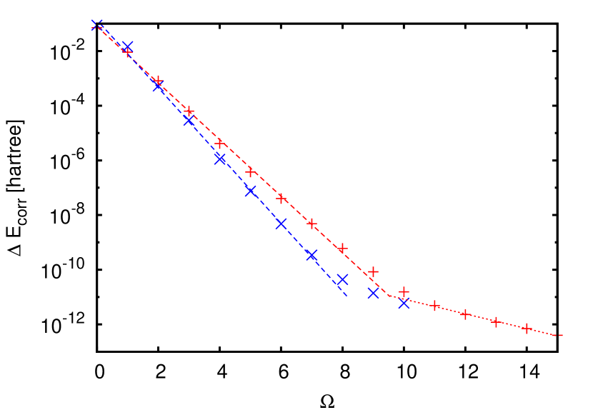
Finally, the convergence of the MP2 and FCCD correlation energies to the complete basis set limit is illustrated in Fig. 1. One can see that the convergence rate of the FCCD energy is slightly faster than of MP2. Another interesting phenomena is the pronounced change in the slope of the curve around $\Omega=8-10$. We do not have a well-justified explanation of this behaviour but it is probably due to the fact that the same nonlinear parameters were used in the SCF and Hylleraas pair functions (without re-optimisation). Other possible contributing factor is the importance of three-particle cusp condition (at the coalescence point of two-electrons and the nucleus) which introduces logarithmic singularities fock54 ; morgan86 in the exact pair functions.

Figure 1: Convergence of the MP2 (red pluses) and FCCD (blue crosses) correlation energy with $\Omega$ for the SCF$(3,7)$ basis set.

The final results of our explicitly correlated calculations are summarised in Table 4. The corresponding results for helium atom and lithium cation/anion are also provided, together with data from Refs. patkowski07 ; bukowski99 ; przybytek09 which used to be the most accurate results available in the literature. The uncertainty of the present data ($\approx$ 1 pE_h) constitutes an improvement of roughly 5 orders of magnitude compared with previous works. The only exception is the lithium ion where the straightforward iteration procedure converges only for small values of $\Omega$. For larger basis sets it becomes oscillatory and finally diverges. This change in the behaviour usually occurred for $n_{\mathrm{a}}$ and $\Omega$ for which the number of basis functions exceeded 400, and prevented us from generating more accurate results.

Table 4: Correlation energies (in mE_h) at different levels of theory for two- and four-electron atomic systems. The present results are shown in the first line while the best GTG results are collected in the second line.

	MP2	FCCD	CCD
He	$-$37.377 474 518 9	$-$42.017 882 917
	$-$37.377 474 52	$-$42.017 71
Li+	$-$40.216 410 043 5	$-$43.490 592 055
	$-$40.216 32	$-$43.490 46
Li-	$-$60.473 978 826 7	$-$71.293 08
	$-$60.473 971	$-$71.293 022	$-$71.266 072
Be	$-$76.358 249 287 3	$-$92.988 771 482
	$-$76.358 245	$-$92.988 754	$-$92.961 031

III.2 Orbital calculations

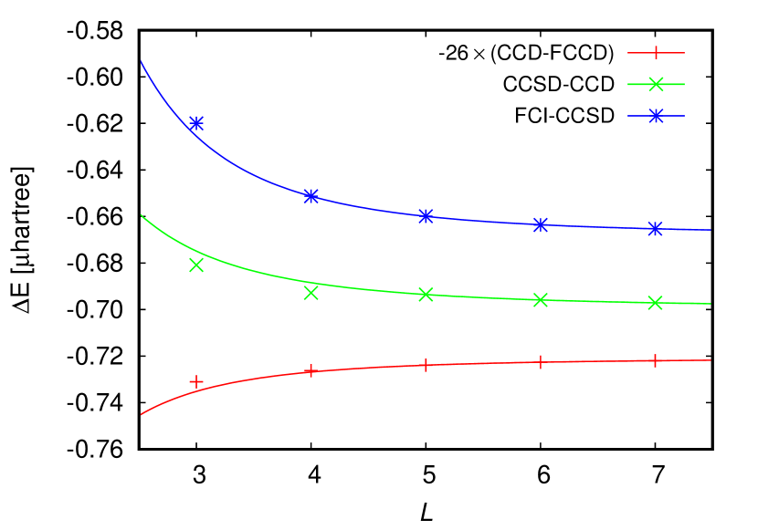
In Table 5 we present results of the calculations of the $\delta_{\mbox{\scriptsize S}}$, $\delta_{\mbox{\scriptsize NF}}$, and $\delta_{\mbox{\scriptsize FCI}}$ corrections using Slater-type orbitals basis sets. The values from $L=3-7$ were extrapolated to the complete basis set limit with help of the following three-point formula

$$A+\frac{B}{(L+1)^{3}}+\frac{C}{(L+1)^{5}}.$$ (19)

which was found to perform best for the FCCD pair energies (in comparison with the corresponding explicitly correlated results). The quality of the extrapolation is illustrated in Fig. 2. One can see that the extrapolation formulae fit the results from $L=4-7$ basis sets quite faithfully. The only exception is the basis set $L=4$ for $\delta_{\mbox{\scriptsize S}}$ which shows a considerable discrepancy making the extrapolated result less reliable.

Table 5: Corrections to the total correlation energy of the beryllium atom calculated within the STOs basis sets. The maximal angular momentum in each basis set is provided in the first column. All values are given in mE_h.

$L$	$\delta_{\mbox{\scriptsize S}}$	$\delta_{\mbox{\scriptsize NF}}$	$\delta_{\mbox{\scriptsize FCI}}$
3	$-$0.680 857	0.028 117	$-$0.619 981
4	$-$0.692 823	0.027 932	$-$0.651 325
5	$-$0.693 542	0.027 843	$-$0.659 907
6	$-$0.695 871	0.027 793	$-$0.663 636
7	$-$0.697 089	0.027 768	$-$0.665 259
$\infty$	$-$0.699 299	0.027 726	$-$0.667 195

Figure 2: Convergence of the $\delta_{\mbox{\scriptsize S}}$, $\delta_{\mbox{\scriptsize NF}}$, and $\delta_{\mbox{\scriptsize FCI}}$ corrections to the complete basis set limit. The correction $\delta_{\mbox{\scriptsize NF}}$ was multiplied by $-26$ to match the scale of the plot.

The extrapolated values of all corrections are given in Table 5. In Table 6 we provide a short summary of the results of the present paper and give the final estimation of the total energy of the beryllium atom. The errors of the respective components are estimated as twice the difference between the extrapolated results and the values in the largest basis set. The total error is about $5\,\mu$E_h ($\approx 1\,$cm^-1) compared with the result of Pachucki and Komasa pachucki04b which can be treated as a reference. This signifies that the present composite method is capable of reaching the accuracy comparable to many spectroscopic measurements. Further in the text we discuss the error in each component given in Table 6 and attempt to isolate the dominant source of the discrepancy. As argued in the previous sections, the uncertainties in the SCF and FCCD energies are essentially negligible at this stage, as indicated in Table 6.

Table 6: Final prediction of the total energy of the beryllium atom. See the main text for details of the uncertainty estimation (shown in parentheses). The values without uncertainty estimation are accurate up to all digits quoted. The reference value is taken from Ref. pachucki04b . All values are given in atomic units.

contribution	value
SCF	$-$14.573 023(4)
FCCD	$-$0.092 989(4)
$\delta_{\mbox{\scriptsize NF}}$	$+$0.000 028(4)
$\delta_{\mbox{\scriptsize S}}$	$-$0.000 699(4)
total CCSD	$-$0.093 660(4)
$\delta_{\mbox{\scriptsize FCI}}$	$-$0.000 667(4)
total energy	$-$14.667 351(6)
reference	$-$14.667 356(4)

The extrapolated value of the non-factorisable doubles correction ($\delta_{\mbox{\scriptsize NF}}$) agrees very well with the result from Table 4 obtained independently with GTG expansions ($\delta_{\mbox{\scriptsize NF}}=0.027\,723$ mE_h). The difference between these values is only about 3 nE_h suggesting that both results are accurate to at least four significant digits. Moreover, as shown in Table 5 the $\delta_{\mbox{\scriptsize NF}}$ correction stabilises quickly with increasing basis set size. Therefore, we expect that in all practical applications it is sufficient to evaluate $\delta_{\mbox{\scriptsize NF}}$ with one-electron basis sets of a decent quality. In the present context, the uncertainty of $\delta_{\mbox{\scriptsize NF}}$ does not contribute significantly to the overall error which is indicated in Table 6.

Unfortunately, the same cannot be said about the singles correction, $\delta_{\mbox{\scriptsize S}}$. As mentioned earlier, the convergence of $\delta_{\mbox{\scriptsize S}}$ towards the complete basis set limit is less regular than for $\delta_{\mbox{\scriptsize NF}}$ or $\delta_{\mbox{\scriptsize FCI}}$ and thus the related extrapolation is not as reliable. Therefore, we expect the extrapolated $\delta_{\mbox{\scriptsize S}}$ correction given in Table 5 to be accurate only to two significant digits. In fact, the present result differs by as much as $5\,\mu$E_h from a more accurate value obtained in Ref. bukowski99 using an explicitly correlated variant of the CCSD theory. We believe that this discrepancy dominates the error in the total energy of the beryllium atom given in Table 6. To confirm this we replace $\delta_{\mbox{\scriptsize S}}$ in Table 6 by the value from Ref. bukowski99 ($-0.705$ mE_h). The total error then drops to about $\approx\,0.1\,$cm^-1 which is an improvement by an order of magnitude. This shows clearly that the dominant error to the total result given in 6 comes from inaccuracies in $\delta_{\mbox{\scriptsize S}}$.

Finally, the correction for the higher-order excitations ($\delta_{\mbox{\scriptsize FCI}}$) is of a similar magnitude as $\delta_{\mbox{\scriptsize S}}$ but exhibits more regular convergence pattern towards the complete basis set limit. While we do not have any reliable result in the literature to compare with directly, a comparison with $\delta_{\mbox{\scriptsize NF}}$ allows us to claim that $\delta_{\mbox{\scriptsize FCI}}$ given in Table 6 is accurate to three significant digits. In other words, the error in $\delta_{\mbox{\scriptsize FCI}}$ is of secondary concern in the present context.

IV Conclusions

In this work we have reported the implementation and the first tests of a new composite method for accurate calculation of energies of many-electron atoms. The dominant contribution to the energy has been calculated by using the explicitly correlated factorisable coupled cluster theory. To expand the pair functions we have employed the Hylleraas basis set and thus eliminated the need for optimisation of the nonlinear parameters at the correlated level. This allowed to compute pair correlation energies of the beryllium atom with error smaller than 1 pE_h, an improvement of several orders of magnitude in comparison with the previous works. The remaining contributions to the total energy have been calculated within the algebraic approximation employing large basis sets composed of Slater-type orbitals.

It is a natural and interesting question of how the present method can be used for heavier atoms retaining or improving the current level of accuracy. In principle, the application of the theory to other many-electron atoms is straightforward. However, the implementation is marred by difficulties related to proper treatment of angular factors originating from $p$, $d$, $\ldots$ reference orbitals. Nonetheless, the Hylleraas basis set has been successfully applied to (high $l$) excited states of the helium atom (see Ref. drake96 and references therein) and we believe that similar extensions are feasible here.

The present level of accuracy can be considerably improved if the correction due to single excitations ($\delta_{\mbox{\scriptsize S}}$) is computed with smaller uncertainty. First-quantised expressions for the explicitly correlated CCSD model (where $\delta_{\mbox{\scriptsize S}}$ is included by construction) are well-known bukowski99 . Unfortunately, their implementation requires four-integrals which are, in general, not available in the Hylleraas basis set. Therefore, it is a considerable challenge to propose an approximate explicitly correlated CCSD model where the most problematic four-electron integrals can be eliminated. This is similar to the idea of Bukowski et al. bukowski99 who proposed the factorisable quadratic CCSD model.

Another problem encountered for heavier atoms is calculation of energy contributions due to higher-excitations from the reference determinant (pentuple, sextuple etc.) The most pragmatic approach is probably to employ Quantum Monte Carlo FCI method booth09 which is capable of probing such large excitation spaces stochastically. With the aforementioned improvements implemented we believe it would be possible to routinely reach the accuracy of $0.1-0.01$ cm^-1 in calculation of the atomic energies. This also requires to include the relativistic and quantum electrodynamics corrections, but as long as the atoms are not too heavy these effects can be accounted for perturbatively. In this case the conventional calculations based on the algebraic approximation are probably sufficient to deliver the desired accuracy.