1- and 3-photon dynamical Casimir effects using nonstationary cyclic qutrit

Abstract

We consider the nonstationary circuit QED setup in which a 3-level artificial atom in the $\Delta$-configuration interacts with a single-mode cavity field of natural frequency $\omega$. It is demonstrated that when some atomic energy level(s) undergoes a weak harmonic modulation, photons can be generated from vacuum via effective 1- and 3-photon transitions, while the atom remains approximately in the ground state. These phenomena occur in the dispersive regime when the modulation frequency is accurately tuned near $\omega$ and $3\omega$, respectively, and the generated field states exhibit strikingly different statistics from the squeezed vacuum state attained in standard cavity dynamical Casimir effect.

I Introduction

The term cavity dynamical Casimir effect (DCE) can be used to denote the class of phenomena that feature the generation of photons from vacuum in some cavity due to the resonant external perturbation of the system parameters, where the cavity serves to produce a resonant enhancement of the DCE rev0 ; rev1 ; nor ; rev2 ; nation ; macri . These phenomena were originally studied in the context of electromagnetic resonators with oscillating walls or containing a macroscopic dielectric medium with time-modulated internal properties zer ; nikonov ; law ; lambrecht ; soh ; maianeto , but later were generalized for other bosonic fields, e. g., phononic excitations of ion chains ions , optomechanical systems opto , cold atoms tito and Bose-Einstein condensates bec1 ; bec2 . For single-mode cavities the main resonance occurs near the modulation frequency $2\omega$, where $\omega$ is the bare cavity frequency, and in the absence of dissipation the average photon number grows exponentially with time pla ; evd , resulting in the squeezed vacuum state with even photon numbers, analogously to the phenomenon of parametric amplification rev0 ; rev2 ; law . The cavity DCE was recently implemented experimentally using a Josephson metamaterial consisting of an array of 250 superconductive interference devices (SQUIDs) embedded in a microwave cavity whose electrical length was modulated by an external magnetic flux meta .

The concept of cavity DCE has been successfully extended to the area of circuit Quantum Electrodynamics (circuit QED) jpcs ; liberato ; zeilinger ; JPA , in which one or several artificial Josephson atoms strongly interact with a microwave field confined in superconducting resonators and waveguides cir1 ; cir2 ; cir3 ; cir4 . The exquisite in situ control over the atomic parameters allows to rapidly modulate the atomic energy levels and the atom-field coupling strength majer ; ge ; ger ; ger1 ; v1 ; v2 ; v3 , enabling the use of artificial atoms as substitutes of the dielectric medium with time-dependent properties. From the viewpoint of a toy model igor , a modulated or oscillating dielectric slab can be imagined as a set of atoms with varying parameters, so ultimately DCE must emerge for a single nonstationary $2$-level atom. Indeed, it was shown that for off-resonant qubit(s) undergoing a weak external perturbation, pairs of photons are generated from vacuum under the modulation frequency $\sim 2\omega$ while the atom(s) remains approximately in the initial state jpcs ; JPA ; igor ; tom . In this scenario the atom plays the role of both the source and real-time detector of DCE, since the (small) atomic transition probability depends on the photon number and in turn affects the photon generation pattern PLAI ; jpcs ; diego . Moreover, the rich nonharmonic spectrum of the composite atom–field system permits the implementation of other phenomena in the nonstationary regime, such as: sideband transitions blais-exp ; schuster ; side2 , anti-dynamical Casimir effect igor ; diego ; lucas ; juan ; werlang , $n$-photon Rabi model nr , generation of entanglement entan ; etc3 , quantum simulations relativistic ; sim ; ger1 and dynamical Lamb effect lamb ; etc1 .

Here we explore theoretically the prospects of implementing nontraditional versions of cavity DCE using 3-level atoms (qutrits) in the cyclic (also known as $\Delta$-) configuration subject to parametric modulation. In this case all the transitions between the atomic levels can occur simultaneously via the cavity field cycl1 ; cycl2 ; cycl3 ; cycl4 , so the total number of excitations is not conserved even upon neglecting the counter-rotating terms (rotating wave approximation). Although prohibited by the electric-dipole selection rules for usual atoms, the $\Delta$-configuration can be implemented for certain artificial atoms in circuit QED cir4 by breaking the inversion symmetry of the potential energy. Our goal is to find new modulation frequencies, exclusive of the cyclic qutrits, that induce photon generation from vacuum without changing appreciably the atomic state.

We find that for the harmonic modulation of some energy level(s) of a dispersive cyclic qutrit, photons can be generated from vacuum for the modulation frequencies $\eta\approx\omega$ and $\eta\approx 3\omega$ while the atom predominantly remains in the ground state. We call these processes 1- and 3-photon DCE because the photons are generated via effective 1- and 3-photon transitions between the system dressed-states, whose rates depend on the product of all the three coupling strengths. We derive an approximate analytical description of the unitary dynamics and illustrate the typical system behavior by solving numerically the Schrödinger equation. In particular, we show that the average photon number and atomic populations display a collapse-revival behavior, and the photon number distributions are completely different from the standard (2-photon) cavity DCE case. Moreover, we solve numerically the Markovian master equation and demonstrate that in the presence of weak dissipation the dissipative dynamics resembles the unitary one for initial times, confirming that our proposal is experimentally feasible.

II Physical system

We consider a single cavity mode of constant frequency $\omega$ that interacts with a qutrit in the cyclic configuration cir4 ; cycl1 ; cycl2 ; cycl3 ; cycl4 , so that all the atomic transitions are allowed via one-photon transitions. The Hamiltonian reads

$$\hat{H}/\hbar=\omega\hat{n}+\sum_{k=1}^{2}E_{k}(t)\hat{\sigma}_{k,k}+\sum_{k=0}^{1}\sum_{l>k}^{2}g_{k,l}(\hat{a}+\hat{a}^{\dagger})(\hat{\sigma}_{l,k}+\hat{\sigma}_{k,l}).$$ (1)

$\hat{a}$ ($\hat{a}^{\dagger}$) is the cavity annihilation (creation) operator and $\hat{n}=\hat{a}^{\dagger}\hat{a}$ is the photon number operator. The atomic eigenenergies are $E_{0}\equiv 0,E_{1}$ and $E_{2}$, the corresponding states are $|\mathbf{k}\rangle$ and we defined $\hat{\sigma}_{k,j}\equiv|\mathbf{k}\rangle\langle\mathbf{j}|$. The constant parameters $g_{k,l}$ denote the coupling strengths between the atomic states $|\mathbf{k}\rangle$ and $|\mathbf{l}\rangle$ mediated by the cavity field. To emphasize the role of the counter-rotating terms (CRT) we rewrite (for $l>k$)

$$g_{k,l}(\hat{a}+\hat{a}^{\dagger})(\hat{\sigma}_{l,k}+\hat{\sigma}_{k,l})\rightarrow g_{k,l}(\hat{a}\hat{\sigma}_{l,k}+c_{k,l}\hat{a}\hat{\sigma}_{k,l}+h.c.),$$

where $c_{k,l}=1$ when the corresponding CRT is taken into account and is zero otherwise.

Utilizing the tunability of Josephson atoms majer ; ge ; ger ; ger1 ; v1 ; v2 ; v3 , we assume that the atomic energy levels can be modulated externally as

$$E_{k}(t)\equiv E_{k}^{(0)}+\varepsilon_{k}\sin(\eta t+\phi_{k})\quad\text{ for}\leavevmode\nobreak\ k=1,2\leavevmode\nobreak\ ,$$

where $\varepsilon_{k}\ll E_{k}^{(0)}$ is the modulation amplitude, $\phi_{k}$ is the associated phase, $E_{k}^{(0)}$ is the bare energy value and $\eta\gtrsim\omega$ is the modulation frequency. We would like to stress that for weak perturbations our approach can be easily generalized to multi-tone modulations or simultaneous perturbation of all the parameters in Hamiltonian (1).

We expand the wavefunction as

$$|\psi(t)\rangle=\sum_{n=0}^{\infty}e^{-it\lambda_{n}}b_{n}(t)\mathcal{F}_{n}(t)|\varphi_{n}\rangle$$ (2)

$$\mathcal{F}_{n}(t)=\exp\left\{\sum_{k=1}^{2}\frac{i\varepsilon_{k}}{\eta}\left[\cos(\eta t+\phi_{k})-1\right]\langle\varphi_{n}|\hat{\sigma}_{k,k}|\varphi_{n}\rangle\right\}.$$

Here $\lambda_{n}$ are the eigenfrequencies of the bare Hamiltonian $\hat{H}_{0}\equiv\hat{H}[\varepsilon_{1}=\varepsilon_{2}=0]$ ($n$ increasing with energy) and $|\varphi_{n}\rangle$ are the corresponding eigenstates (dressed-states). $b_{n}(t)$ denotes the slowly-varying probability amplitude of the state $|\varphi_{n}\rangle$ and $\mathcal{F}_{n}(t)\approx 1$ is a rapidly oscillating function with a small amplitude.

After substituting Eq. (2) into the Schrödinger equation, to the first order in $\varepsilon_{1}$ and $\varepsilon_{2}$ we obtain the differential equation

$$\dot{b}_{n}=\sum\limits_{m\neq n}b_{m}\left[\Theta_{m;n}^{\ast}e^{it\left(\lambda_{n}-\lambda_{m}-\eta\right)}-\Theta_{n;m}e^{-it\left(\lambda_{m}-\lambda_{n}-\eta\right)}\right]$$ (3)

that describes transitions between the dressed-states $|\varphi_{n}\rangle$ and $|\varphi_{m}\rangle$ with the transition rate $|\Theta_{n;m}|$, where

$$\Theta_{n;m}\equiv\frac{1}{2}\sum_{k=1}^{2}\varepsilon_{k}e^{i\phi_{k}}\langle\varphi_{n}|\hat{\sigma}_{k,k}|\varphi_{m}\rangle.$$ (4)

The transition $|\varphi_{n}\rangle\leftrightarrow|\varphi_{m}\rangle$ occurs when the modulation frequency is resonantly tuned to $\eta_{r}=|\lambda_{m}-\lambda_{n}|+\Delta\nu$, where $\Delta\nu$ denotes a small shift JPA dependent on $\varepsilon_{1},\varepsilon_{2}$ due to the rapidly-oscillating terms that were neglected in Eq. (3) (in this paper we adjust $\Delta\nu$ numerically). By writing the interaction-picture wavefunction as $|\psi_{I}(t)\rangle=\sum_{n}b_{n}(t)|\varphi_{n}\rangle$ one can cast Eq. (3) as a dressed-picture effective Hamiltonian

$$\hat{H}_{ef}(t)=-i\sum_{n,m\neq n}\Theta_{m;n}|\varphi_{m}\rangle\langle\varphi_{n}|e^{-it\left(\lambda_{n}-\lambda_{m}-\eta\right)}+h.c.$$

Since we focus on transitions in which the atom is minimally disturbed, we consider the dispersive regime

$$|\Delta_{1}|,|\Delta_{2}|,|\Delta_{1}+\Delta_{2}|\gg\sqrt{n_{\max}}\max(g_{k,l})\leavevmode\nobreak\ ,$$

where $n_{\max}$ is the maximum number of the system excitations and the bare detunings are defined as

$$\Delta_{1}\equiv\omega-E_{1}^{(0)},\leavevmode\nobreak\ \Delta_{2}\equiv\omega-(E_{2}^{(0)}-E_{1}^{(0)}),\leavevmode\nobreak\ \Delta_{3}\equiv\Delta_{1}+\Delta_{2}.$$

Denoting by $|\zeta_{k}\rangle$ the dressed-states in which the atom is predominantly in the ground state, from the standard perturbation theory we find

$$|\zeta_{k}\rangle \approx |\mathbf{0},k\rangle+\frac{c_{0,1}g_{0,1}^{2}\sqrt{k(k-1)}}{2\Delta_{1}\omega}|\mathbf{0},k-2\rangle$$

$$+\frac{g_{0,1}\sqrt{k}}{\Delta_{1}}|\mathbf{1},k-1\rangle-\frac{c_{0,1}g_{0,1}\sqrt{k+1}}{2\omega-\Delta_{1}}|\mathbf{1},k+1\rangle$$

$$-\frac{c_{1,2}g_{0,1}g_{1,2}k}{\Delta_{1}(2\omega-\Delta_{3})}|\mathbf{2},k\rangle+\frac{g_{0,1}g_{1,2}\sqrt{k(k-1)}}{\Delta_{1}\Delta_{3}}|\mathbf{2},k-2\rangle$$

$$-\frac{g_{0,2}\sqrt{k}}{\omega-\Delta_{3}}|\mathbf{2},k-1\rangle-\frac{c_{0,2}g_{0,2}\sqrt{k+1}}{3\omega-\Delta_{3}}|\mathbf{2},k+1\rangle$$

where $|\mathbf{j},k\rangle\equiv|\mathbf{j}\rangle_{atom}\otimes|k\rangle_{field}$ and $k\geq 0$. The corresponding eigenfrequencies are (neglecting constant shifts)

$$\Lambda_{k}\approx\omega_{ef}k+\alpha k^{2}$$ (6)

with the effective cavity frequency and the one-photon Kerr nonlinearity, respectively,

$$\omega_{ef} \equiv \omega+\frac{g_{0,1}^{2}}{\Delta_{1}}\left(1-\frac{g_{1,2}^{2}}{\Delta_{1}\Delta_{3}}\right)-\frac{g_{0,2}^{2}}{\omega-\Delta_{3}}$$

$$-\frac{c_{0,1}g_{0,1}^{2}}{2\omega-\Delta_{1}}-\frac{c_{0,2}g_{0,2}^{2}}{3\omega-\Delta_{3}}$$

$$\alpha \equiv \frac{g_{0,1}^{2}}{\Delta_{1}^{2}}\left(\frac{g_{1,2}^{2}}{\Delta_{3}}-\frac{g_{0,1}^{2}}{\Delta_{1}}+\frac{c_{0,1}g_{0,1}^{2}}{2\omega}-\frac{c_{1,2}g_{1,2}^{2}}{2\omega-\Delta_{3}}\right.$$

$$\left.+\frac{g_{0,2}^{2}}{\omega-\Delta_{3}}+\frac{c_{0,1}g_{0,1}^{2}}{2\omega-\Delta_{1}}+\frac{c_{0,2}g_{0,2}^{2}}{3\omega-\Delta_{3}}\right).$$

In the Appendix A we present the complete expressions for the eigenstates and eigenvalues obtained from the 2- and 4-order perturbation theory, respectively.

III 1- and 3-photon DCE

The lowest-order phenomena that occur exclusively for cyclic qutrits depend on the combination $g_{0,1}g_{1,2}g_{0,2}$, so we define $G^{3}\equiv g_{0,1}g_{1,2}g_{0,2}/2$. Indeed, for $g_{0,2}=0$ we recover the ladder configuration, for $g_{0,1}=0$ the $\Lambda$- configuration and for $g_{1,2}=0$ the V-configuration. After substituting the dressed-states (9) into Eq. (4) we find that one such effect is the three-photon transition between the states $|\zeta_{k}\rangle$ and $|\zeta_{k+3}\rangle$. To the lowest order the respective transition rate reads

$$\Theta_{k;k+3}^{(\zeta)}=G^{3}\sqrt{\frac{(k+3)!}{k!}}\left[\varepsilon_{1}q_{1}e^{i\phi_{1}}-\varepsilon_{2}q_{2}e^{i\phi_{2}}\right],$$ (7)

where the $k$-independent parameters are

$$q_{1} = \frac{c_{0,2}}{\Delta_{1}\left(3\omega-\Delta_{3}\right)\left(3\omega-\Delta_{1}\right)}$$

$$+\frac{c_{0,1}c_{1,2}}{\left(2\omega-\Delta_{1}\right)\left(\omega-\Delta_{3}\right)\left(\omega+\Delta_{1}\right)}$$

$$q_{2} = \frac{c_{0,2}}{\Delta_{1}\Delta_{3}\left(3\omega-\Delta_{3}\right)}$$

$$+\frac{c_{0,1}c_{1,2}}{\left(2\omega-\Delta_{1}\right)\left(\omega-\Delta_{3}\right)\left(4\omega-\Delta_{3}\right)}\leavevmode\nobreak\ .$$

We see that this effect, corresponding roughly to the transitions $|\mathbf{0},k\rangle\leftrightarrow|\mathbf{0},k+3\rangle\leftrightarrow|\mathbf{0},k+6\rangle\leftrightarrow\cdots$, relies on the CRT: either $c_{0,2}$ must be nonzero, or the product $c_{0,1}c_{1,2}$.

The second effect allowed by the cyclic configuration is the one-photon transition between the states $|\zeta_{k}\rangle$ and $|\zeta_{k+1}\rangle$, or roughly $|\mathbf{0},k\rangle\leftrightarrow|\mathbf{0},k+1\rangle\leftrightarrow|\mathbf{0},k+2\rangle\leftrightarrow\cdots$. We obtain to the lowest order

$$\Theta_{k;k+1}^{(\zeta)}=G^{3}\sqrt{k+1}\left[\varepsilon_{1}Q_{1}(k)e^{i\phi_{1}}-\varepsilon_{2}Q_{2}(k)e^{i\phi_{2}}\right],$$ (8)

where we defined $k$-dependent functions

$$Q_{1}(k) = \frac{1}{\Delta_{1}(\omega-\Delta_{1})}\left(\frac{c_{1,2}c_{0,2}(k+1)}{3\omega-\Delta_{3}}+\frac{k}{\omega-\Delta_{3}}\right)$$

$$-\frac{c_{0,1}c_{0,2}(k+2)}{(2\omega-\Delta_{1})(3\omega-\Delta_{3})(3\omega-\Delta_{1})}$$

$$-\frac{c_{1,2}k}{\Delta_{1}(\omega-\Delta_{3})(\omega+\Delta_{1})}-\frac{c_{0,1}}{(\omega-\Delta_{1})(2\omega-\Delta_{1})}$$

$$\times\left(\frac{c_{1,2}c_{0,2}(k+2)}{3\omega-\Delta_{3}}+\frac{k+1}{\omega-\Delta_{3}}\right)$$

$$Q_{2}(k) = \frac{1}{(2\omega-\Delta_{3})(\omega-\Delta_{3})}\left(\frac{c_{0,1}(k+1)}{2\omega-\Delta_{1}}-\frac{c_{1,2}k}{\Delta_{1}}\right)$$

$$+\frac{c_{0,1}c_{1,2}c_{0,2}(k+2)}{(2\omega-\Delta_{1})(4\omega-\Delta_{3})(3\omega-\Delta_{3})}$$

$$+\frac{k}{\Delta_{1}\Delta_{3}(\omega-\Delta_{3})}+\frac{c_{0,2}}{(2\omega-\Delta_{3})(3\omega-\Delta_{3})}$$

$$\times\left(\frac{c_{0,1}(k+2)}{2\omega-\Delta_{1}}-\frac{c_{1,2}(k+1)}{\Delta_{1}}\right).$$

We see that for $k>0$ (nonvacuum field states) the CRT are not required for this effect, but for the photon generation from vacuum either $c_{0,1}$ or the product $c_{1,2}c_{0,2}$ must be nonzero. In analogy to the generation of photon pairs in the standard DCE, we call the above effects 3- and 1-photon DCE, respectively.

As seen from Eqs. (7) and (8), to induce the 1- and 3-photon DCE it is sufficient to modulate just one of the energy levels, yet the simultaneous modulation of both $E_{1}$ and $E_{2}$ can increase the transition rate provided the phase difference $(\phi_{1}-\phi_{2})$ is properly adjusted. However, for constant modulation frequency the photon generation from vacuum is limited due to the resonance mismatch for multiphoton dressed states. Indeed, from Eq. (6) we have

$$\Lambda_{k+J}-\Lambda_{k}=\left(\omega_{ef}+J\alpha\right)J+(2\alpha J)k\,,$$

where $J=1,3$. Assuming realistically that $g_{l,k}$ and $\varepsilon_{j}$ are all of the same order of magnitude, we note that $|\alpha|\gtrsim|\Theta_{k;k+J}^{(\zeta)}|$ for $k\sim 1$. Hence for constant $\eta_{J}\simeq\Lambda_{J}-\Lambda_{0}$ (adjusted to generate photons from vacuum) the coupling between the states $|\zeta_{k}\rangle\rightarrow|\zeta_{k+J}\rangle$ goes off resonance as $k$ increases and we expect a limited photon production. We note that several methods to enhance the photon generation were proposed in similar setups, e.g., multi-tone modulations jpcs ; diego , time-varying modulation frequency including effective Landau-Zener transitions palermo and optimum control strategies optcontrol .

IV Discussion and conclusions

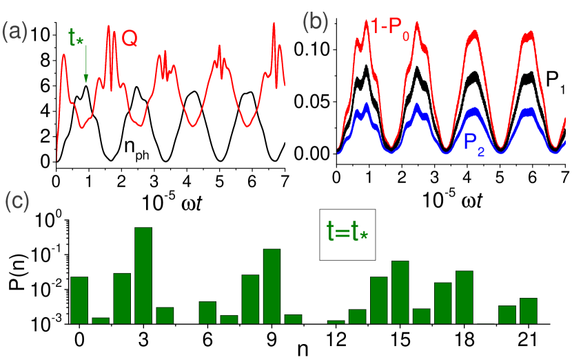
Figure 1: (color online) System behavior for 3-photon DCE. a) Dynamics of the average photon number $n_{ph}$ and the Mandel’s $Q$-factor. b) Dynamics of the atomic populations: the probability that atom leaves the initial state is $\lesssim 12\%$. c) Photon statistics $P(n)=\mathrm{Tr}(\hat{\rho}|n\rangle\langle n|)$ for the time instant $\omega t_{\ast}=0.91\times 10^{5}$ [marked by the green arrow in (a)], where $\hat{\rho}$ is the total density operator. Notice the local peaks at $n=3k$, asserting the effective 3-photon nature of the process.

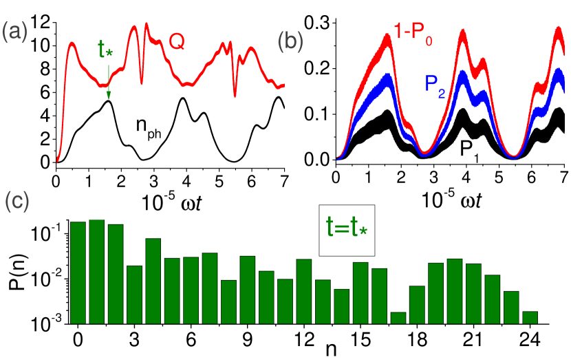
Figure 2: (color online) System behavior for 1-photon DCE. Similar to Fig. 1. The probability that the atom leaves the initial state is now $\lesssim 30\%$. For $\omega t_{\ast}=1.61\times 10^{5}$ (panel c) the photon statistics lacks local peaks, indicating that the photons are generated via effective 1-photon transitions.

To confirm our analytic predictions we solve numerically the Schrödinger equation for the Hamiltonian (1) considering the initial state $|\mathbf{0},0\rangle$ (which is approximately equal to the system ground state in our regime of parameters) and feasible coupling constants $g_{0,1}/\omega=5\times 10^{-2}$, $g_{1,2}/\omega=6\times 10^{-2}$ and $g_{0,2}/\omega=3\times 10^{-2}$ (including all the CRT, $c_{l,k}=1$). For the sake of illustration we consider the sole modulation of $E_{2}$, setting $\varepsilon_{1}=0$ and $\varepsilon_{2}=7\times 10^{-2}E_{2}^{(0)}$. In Fig. 1 we illustrate the 3-photon DCE for the detunings $\Delta_{1}/\omega=0.464$, $\Delta_{2}/\omega=0.106$ and modulation frequency $\eta/\omega=3.0037$. We show the average photon number $n_{ph}=\langle\hat{a}^{\dagger}\hat{a}\rangle$, the Mandel’s factor $Q=[\langle(\Delta\hat{n})^{2}\rangle-n_{ph}]/n_{ph}$ (that quantifies the spread of the photon number distribution, being $Q=1+2n_{ph}$ for the squeezed vacuum state) and the atomic populations $P_{k}=\langle\hat{\sigma}_{k,k}\rangle$. We also show the photon number distribution at the time instant $\omega t_{\ast}=0.91\times 10^{5}$ (when $n_{ph}$ is maximum), confirming that the photon generation occurs via effective 3-photon processes. We observe that for $t=t_{\ast}$ the photon statistics does not show special behavior around $n\approx n_{ph}$. The average photon number and the atomic populations exhibits a collapse-revival behavior due to increasingly off-resonant couplings between the probability amplitudes $b_{m}$ in Eq. (3). Moreover, during the collapses [$n_{ph},(1-P_{0})\approx 0$] the Mandel’s factor is very large, $Q\gg 1,n_{ph}$, which is typical of hyper-Poissonian states that have long tails of distribution with very low (but not negligible) probabilities PLAI .

In Fig. 2 we perform a similar analysis for the 1-photon DCE, setting the parameters $\Delta_{1}/\omega=0.362$, $\Delta_{2}/\omega=0.51$ and $\eta/\omega=0.9978$. The qualitative behavior of $n_{ph}$, $Q$ and the atomic populations is similar to the previous case, but the photon number distribution is completely different, as illustrated in the panel (c) for $\omega t_{\ast}=1.61\times 10^{5}$. Now all the photon states are populated (as expected for an effective 1-photon process), and the $Q$-factor is always larger that $n_{ph}$ due to the larger spread of the distribution. As in the previous example, there are no special features in the photon statistics for $n\approx n_{ph}$, and one has similar probabilities of detecting any value ranging from 3 to 20 photons.

To assess the experimental feasibility of our proposal we solve numerically the phenomenological Markovian master equation for the density operator $\hat{\rho}$ cycl2 ; cycl4

$$\dot{\rho}=\frac{1}{i\hbar}[\hat{H},\hat{\rho}]+\kappa\mathcal{L}[\hat{a}]+\sum_{k=0}^{1}\sum_{l>k}^{2}\gamma_{k,l}\mathcal{L}[\hat{\sigma}_{k,l}]+\sum_{k=1}^{2}\gamma_{k}^{(\phi)}\mathcal{L}[\hat{\sigma}_{k,k}]\,,$$

where $\mathcal{L}[\hat{O}]\equiv\hat{O}\hat{\rho}\hat{O}^{\dagger}-\hat{O}^{\dagger}\hat{O}\hat{\rho}/2-\hat{\rho}\hat{O}^{\dagger}\hat{O}/2$ is the Lindblad superoperator, $\kappa$ is the cavity relaxation rate and $\gamma_{k,l}$ ($\gamma_{k}^{(\phi)}$) are the atomic relaxation (pure dephasing) rates. Notice that related works demonstrated that for $g_{k,l}/\omega<10^{-1}$ and initial times this approach is a good approximation to a more rigorous microscopic model of dissipation diego ; werlang ; palermo . Typical behavior of 3-photon DCE under unitary and dissipative evolutions is illustrated in Fig. 3, where we set $\Delta_{1}/\omega=0.24$, $\Delta_{2}/\omega=-0.132$, $\eta/\omega=3.0269$ solv and feasible dissipative parameters $\gamma_{k,l}=\gamma_{k}^{(\phi)}=g_{0,1}\times 10^{-3}$ and $\kappa=g_{0,1}\times 10^{-4}$ (other parameters are as in Fig. 1). It is seen that for initial times the dissipative dynamics resembles the unitary one, indicating that our predictions could be verified in realistic circuit QED systems.

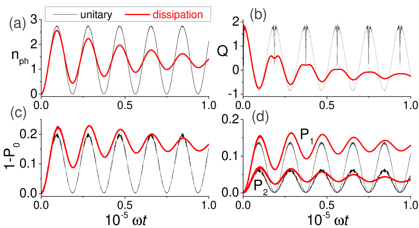
Figure 3: (color online) Dissipative 3-photon DCE. Behavior of $n_{ph}$, $Q$ and $P_{k}$ under unitary (black thin lines) and dissipative (red thick lines) evolutions. For initial times (till the first maximum of $n_{ph}$) the effects of dissipation are small; for larger times the dissipation strongly affects the dynamics, but the main qualitative features persist.

In conclusion, we showed that for an artificial cyclic qutrit coupled to a single-mode cavity one can induce effective 1- and 3-photon transitions between the system dressed-states in which the atom remains approximately in the ground state. These effects occur in the dispersive regime of light-matter interaction for external modulation of some system parameter(s) with frequencies $\eta\approx\omega$ and $\eta\approx 3\omega$, respectively. We evaluated the associated transition rates assuming the modulation of one or both excited energy-levels of the atom, and our method can be easily extended to the perturbation of all the parameters in the Hamiltonian. For constant modulation frequency the average photon number and the atomic populations exhibit a collapse-revival behavior with a limited photon generation due to effective Kerr nonlinearities. The photon statistics is strikingly different from the standard (2-photon) DCE case, for which a squeezed vacuum state would be generated. Although we focused on transitions that avoid exciting the atom, our approach can be applied to study other uncommon transitions allowed by $\Delta$-atoms. Hence this study indicates viable alternatives to engineer effective interactions in nonstationary circuit QED using cyclic qutrits.

Appendix A Full expressions for the dressed states

For the purpose of this paper it is sufficient to calculate the eigenstates of the Hamiltonian $\hat{H}_{0}$ using the second-order perturbation theory. In the dispersive regime we obtain

$$|\zeta_{k}\rangle = \mathcal{N}_{k}\left[|\mathbf{0},k\rangle+\frac{g_{0,1}\sqrt{k}}{\Delta_{1}}|\mathbf{1},k-1\rangle-\frac{c_{0,1}g_{0,1}\sqrt{k+1}}{2\omega-\Delta_{1}}|\mathbf{1},k+1\rangle-\frac{g_{0,2}\sqrt{k}}{\omega-\Delta_{3}}|\mathbf{2},k-1\rangle-\frac{c_{0,2}g_{0,2}\sqrt{k+1}}{3\omega-\Delta_{3}}|\mathbf{2},k+1\rangle\right.$$ (9)

$$+\left(\frac{c_{0,1}g_{0,1}^{2}}{2\omega-\Delta_{1}}+\frac{c_{0,2}g_{0,2}^{2}}{3\omega-\Delta_{3}}\right)\frac{\sqrt{(k+1)(k+2)}}{2\omega}|\mathbf{0},k+2\rangle+\left(\frac{c_{0,1}g_{0,1}^{2}}{\Delta_{1}}-\frac{c_{0,2}g_{0,2}^{2}}{\omega-\Delta_{3}}\right)\frac{\sqrt{k(k-1)}}{2\omega}|\mathbf{0},k-2\rangle$$

$$+\left(\frac{c_{1,2}c_{0,2}(k+1)}{3\omega-\Delta_{3}}+\frac{k}{\omega-\Delta_{3}}\right)\frac{g_{1,2}g_{0,2}}{\omega-\Delta_{1}}|\mathbf{1},k\rangle+\left(\frac{c_{0,1}(k+1)}{2\omega-\Delta_{1}}-\frac{c_{1,2}k}{\Delta_{1}}\right)\frac{g_{0,1}g_{1,2}}{2\omega_{0}-\Delta_{3}}|\mathbf{2},k\rangle$$

$$+\frac{c_{0,2}g_{1,2}g_{0,2}\sqrt{(k+1)(k+2)}}{(3\omega-\Delta_{3})(3\omega-\Delta_{1})}|\mathbf{1},k+2\rangle-\frac{c_{1,2}g_{1,2}g_{0,2}\sqrt{k(k-1)}}{(\omega-\Delta_{3})(\omega_{0}+\Delta_{1})}|\mathbf{1},k-2\rangle$$

$$\left.+\frac{c_{0,1}c_{1,2}g_{0,1}g_{1,2}\sqrt{(k+1)(k+2)}}{(2\omega_{0}-\Delta_{1})(4\omega-\Delta_{3})}|\mathbf{2},k+2\rangle+\frac{g_{0,1}g_{1,2}\sqrt{k(k-1)}}{\Delta_{1}\Delta_{3}}|\mathbf{2},k-2\rangle\right],$$

where $\mathcal{N}_{k}=1+O[(g_{0}/\Delta_{1})^{2}]$ is the normalization constant whose value does not appear in our final (lowest-order) expressions.

For the eigenenergy corresponding to the state $|\zeta_{k}\rangle$ we need to use the fourth-order perturbation theory to account for the effective Kerr-nonlinearity. We get

$$\Lambda_{k}=\omega k+L_{1}(k)+L_{2}(k)$$

$$L_{1}(k)\equiv\left(\delta_{1}-\delta_{2}-c_{0,1}\delta_{3}-c_{0,2}\delta_{4}\right)k-\left(c_{0,1}\delta_{3}+c_{0,2}\delta_{4}\right)$$

$$L_{2}(k)\equiv\left[\delta_{1}\beta_{1}(k)-\delta_{2}\beta_{2}(k)\right]k-\left[c_{0,1}\delta_{3}\beta_{3}(k)+c_{0,2}\delta_{4}\beta_{4}(k)\right]\left(k+1\right).$$

We defined the shifts $\delta_{1}=g_{0,1}^{2}/\Delta_{1}$, $\delta_{2}=g_{0,2}^{2}/(\omega-\Delta_{3})$, $\delta_{3}=g_{0,1}^{2}/(2\omega-\Delta_{1})$, $\delta_{4}=g_{0,2}^{2}/(3\omega-\Delta_{3})$, $\delta_{5}=g_{1,2}^{2}/(2\omega-\Delta_{3})$, $\delta_{6}=g_{1,2}^{2}/(\omega-\Delta_{1})$. Other dimensionless functions of $k$ are defined as

$$\beta_{1}(k)\equiv\left(\delta_{1}-c_{0,2}\delta_{2}\right)\frac{c_{0,1}\left(k-1\right)}{2\omega}+\frac{g_{1,2}^{2}\left(k-1\right)}{\Delta_{1}\Delta_{3}}+c_{1,2}\delta_{5}\left(\frac{c_{0,1}\left(k+1\right)}{2\omega-\Delta_{1}}-\frac{k}{\Delta_{1}}\right)-\frac{L_{1}(k)}{\Delta_{1}}$$

$$\beta_{2}(k)\equiv\left(c_{0,1}\delta_{1}-\delta_{2}\right)\frac{c_{0,2}\left(k-1\right)}{2\omega}-\frac{c_{1,2}g_{1,2}^{2}\left(k-1\right)}{\left(\omega-\Delta_{3}\right)\left(\omega+\Delta_{1}\right)}+\delta_{6}\left(\frac{c_{1,2}c_{0,2}\left(k+1\right)}{3\omega-\Delta_{3}}+\frac{k}{\omega-\Delta_{3}}\right)+\frac{L_{1}(k)}{\omega-\Delta_{3}}$$

$$\beta_{3}(k)\equiv\left(\delta_{3}+c_{0,2}\delta_{4}\right)\frac{k+2}{2\omega}+\delta_{5}\left(\frac{\left(k+1\right)}{2\omega_{0}-\Delta_{1}}-\frac{c_{1,2}k}{\Delta_{1}}\right)+\frac{c_{1,2}g_{1,2}^{2}\left(k+2\right)}{\left(2\omega-\Delta_{1}\right)\left(4\omega-\Delta_{3}\right)}+\frac{L_{1}(k)}{2\omega-\Delta_{1}}$$

$$\beta_{4}(k)\equiv\left(c_{0,1}\delta_{3}+\delta_{4}\right)\frac{k+2}{2\omega}+c_{1,2}\delta_{6}\left(\frac{c_{1,2}\left(k+1\right)}{3\omega-\Delta_{3}}+\frac{k}{\omega-\Delta_{3}}\right)+\frac{g_{1,2}^{2}\left(k+2\right)}{\left(3\omega-\Delta_{3}\right)\left(3\omega-\Delta_{1}\right)}+\frac{L_{1}(k)}{3\omega-\Delta_{3}}.$$

References

- (1) V. V. Dodonov, Nonstationary Casimir Effect and analytical solutions for quantum fields in cavities with moving boundaries, in Modern Nonlinear Optics, Advances in Chemical Physics Series, Vol. 119, part 1, edited by M. W. Evans (Wiley, New York, 2001), pp. 309–394.
- (2) V. V. Dodonov, Current status of the dynamical Casimir effect, Phys. Scr. 82, 038105 (2010).
- (3) J. R. Johansson, G. Johansson, C. M. Wilson, and F. Nori, Dynamical Casimir effect in superconducting microwave circuits, Phys. Rev. A 82, 052509 (2010).
- (4) P. D. Nation, J. R. Johansson, M. P. Blencowe, and F. Nori, Colloquium: Stimulating uncertainty: Amplifying the quantum vacuum with superconducting circuits, Rev. Mod. Phys. 84, 1 (2012).
- (5) P. D. Nation, J. Suh, and M. P. Blencowe, Ultrastrong optomechanics incorporating the dynamical Casimir effect, Phys. Rev. A 93, 022510 (2016).
- (6) V. Macrì, A. Ridolfo, O. Di Stefano, A. F. Kockum, F. Nori, and Salvatore Savasta, Nonperturbative Dynamical Casimir Effect in Optomechanical Systems: Vacuum Casimir-Rabi Splittings, Phys. Rev. X 8, 011031 (2018).
- (7) V. V. Dodonov and A. B. Klimov, Long-time asymptotics of a quantized electromagnetic field in a resonator with oscillating boundary, Phys. Lett. A 167, 309 (1992).
- (8) V. V. Dodonov, A. B. Klimov and D. E. Nikonov, Quantum phenomena in nonstationary media, Phys. Rev. A 47, 4422 (1993).
- (9) C. K. Law, Effective Hamiltonian for the radiation in a cavity with a moving mirror and a time-varying dielectric medium, Phys. Rev. A 49, 433 (1994).
- (10) A. Lambrecht, M.-T. Jaekel and S. Reynaud, Motion Induced Radiation from a Vibrating Cavity, Phys. Rev. Lett. 77, 615 (1996).
- (11) J.-Y. Ji, H.-H. Jung, J.-W. Park, and K.-S. Soh, Production of photons by the parametric resonance in the dynamical Casimir effect, Phys. Rev. A 56, 4440 (1997).
- (12) D. F. Mundarain and P. A. Maia Neto, Quantum radiation in a plane cavity with moving mirrors, Phys. Rev. A 57, 1379 (1998).
- (13) N. Trautmann and P. Hauke, Quantum simulation of the dynamical Casimir effect with trapped ions, New J. Phys. 18, 043029 (2016).
- (14) A. Motazedifard, M. H. Naderi and R. Roknizadeh, Dynamical Casimir effect of phonon excitation in the dispersive regime of cavity optomechanics, J. Opt. Soc. Am. B 34, 642 (2017).
- (15) V. V. Dodonov and J. T. Mendonça, Dynamical Casimir effect in ultra-cold matter with a time-dependent effective charge, Phys. Scr. T160, 014008 (2014).
- (16) I. Carusotto, R. Balbinot, A. Fabbri, and A. Recati, Density correlations and analog dynamical Casimir emission of Bogoliubov phonons in modulated atomic Bose-Einstein condensates, Eur. Phys. J. D 56, 391 (2010).
- (17) J. C. Jaskula, G. B. Partridge, M. Bonneau, R. Lopes, J. Ruaudel, D. Boiron, C. I. Westbrook, Acoustic Analog to the Dynamical Casimir Effect in a Bose-Einstein Condensate, Phys. Rev. Lett. 109, 220401 (2012).
- (18) V. V. Dodonov, Photon creation and excitation of a detector in a cavity with a resonantly vibrating wall, Phys. Lett. A 207, 126 (1995).
- (19) A.V. Dodonov, E.V. Dodonov, and V.V. Dodonov, Photon generation from vacuum in nondegenerate cavities with regular and random periodic displacements of boundaries, Phys. Lett. A 317, 378 (2003).
- (20) P. Lähteenmäki, G. S. Paraoanu, J. Hassel, and P. J. Hakonen, Dynamical Casimir effect in a Josephson metamaterial, Proc. Natl. Acad. Sci. USA 110, 4234 (2013).
- (21) A. V. Dodonov, Photon creation from vacuum and interactions engineering in nonstationary circuit QED, J. Phys.: Conf. Ser. 161, 012029 (2009).
- (22) S. De Liberato, D. Gerace, I. Carusotto, and C. Ciuti, Extracavity quantum vacuum radiation from a single qubit, Phys. Rev. A 80, 053810 (2009).
- (23) T. Fujii, S. Matsuo, N. Hatakenaka, S. Kurihara, and A. Zeilinger, Quantum circuit analog of the dynamical Casimir effect, Phys. Rev. B 84, 174521 (2011).
- (24) A. V. Dodonov, Analytical description of nonstationary circuit QED in the dressed-states basis, J. Phys. A: Math. Theor. 47, 285303 (2014).
- (25) J. Q. You and F. Nori, Atomic physics and quantum optics using superconducting circuits, Nature (London) 474, 589 (2011).
- (26) M. H. Devoret and R. J. Schoelkopf, Superconducting circuits for quantum information: An outlook, Science 339, 1169 (2013).
- (27) G. Wendin, Quantum information processing with superconducting circuits: A review, Rep. Prog. Phys. 80, 106001 (2017).
- (28) X. Gu, A. F. Kockum, A. Miranowicz, Yu-xi Liu, and F. Nori, Microwave photonics with superconducting quantum circuits, Phys. Rep. 718-719, 1 (2017).
- (29) J. Majer, J. M. Chow, J. M. Gambetta, J. Koch, B. R. Johnson, J. A. Schreier, L. Frunzio, D. I. Schuster, A. A. Houck, A. Wallraff, A. Blais, M. H. Devoret, S. M. Girvin, and R. J. Schoelkopf, Coupling superconducting qubits via a cavity bus, Nature 449, 443 (2007).
- (30) M. Hofheinz, H. Wang, M. Ansmann, R. C. Bialczak, E. Lucero, M. Neeley, A. D. O’Connell, D. Sank, J. Wenner, J. M. Martinis, and A. N. Cleland, Synthesizing arbitrary quantum states in a superconducting resonator, Nature 459, 546 (2009).
- (31) L. DiCarlo, J. M. Chow, J. M. Gambetta, L. S. Bishop, B. R. Johnson, D. I. Schuster, J. Majer, A. Blais, L. Frunzio, S. M. Girvin, and R. J. Schoelkopf, Demonstration of two-qubit algorithms with a superconducting quantum processor, Nature 460, 240 (2009).
- (32) J. Li, M. P. Silveri, K. S. Kumar, J. -M. Pirkkalainen, A. Vepsäläinen, W. C. Chien, J. Tuorila, M. A. Sillanpää, P. J. Hakonen, E. V. Thuneberg, and G. S. Paraoanu, Motional averaging in a superconducting qubit, Nat. Commun. 4, 1420 (2013).
- (33) S. J. Srinivasan, A. J. Hoffman, J. M. Gambetta, and A. A. Houck, Tunable Coupling in Circuit Quantum Electrodynamics Using a Superconducting Charge Qubit with a V-Shaped Energy Level Diagram, Phys. Rev. Lett. 106, 083601 (2011).
- (34) Y. Chen, C. Neill, P. Roushan, N. Leung, M. Fang, R. Barends, J. Kelly, B. Campbell, Z. Chen, B. Chiaro, A. Dunsworth, E. Jeffrey, A. Megrant, J. Y. Mutus, P. J. J. O’Malley, C. M. Quintana, D. Sank, A. Vainsencher, J. Wenner, T. C. White, M. R. Geller, A. N. Cleland, and J. M. Martinis, Qubit Architecture with High Coherence and Fast Tunable Coupling, Phys. Rev. Lett. 113, 220502 (2014).
- (35) S. Zeytinoğlu, M. Pechal, S. Berger, A. A. Abdumalikov, Jr., A. Wallraff, and S. Filipp, Microwave-induced amplitude- and phase-tunable qubit-resonator coupling in circuit quantum electrodynamics, Phys. Rev. A 91, 043846 (2015).
- (36) I. M. de Sousa and A. V. Dodonov, Microscopic toy model for the cavity dynamical Casimir effect, J. Phys. A: Math. Theor. 48, 245302 (2015).
- (37) E. L. S. Silva and A. V. Dodonov, Analytical comparison of the first- and second-order resonances for implementation of the dynamical Casimir effect in nonstationary circuit QED, J. Phys. A: Math. Theor. 49, 495304 (2016).
- (38) A. V. Dodonov and V. V. Dodonov, Strong modifications of the field statistics in the cavity dynamical Casimir effect due to the interaction with two-level atoms and detectors, Phys. Lett. A 375, 4261 (2011).
- (39) D. S. Veloso and A. V. Dodonov, Prospects for observing dynamical and antidynamical Casimir effects in circuit QED due to fast modulation of qubit parameters, J. Phys. B: At. Mol. Opt. Phys. 48, 165503 (2015).
- (40) J. D. Strand, M. Ware, F. Beaudoin, T. A. Ohki, B. R. Johnson, A. Blais, and B. L. T. Plourde, First-order sideband transitions with flux-driven asymmetric transmon qubits, Phys. Rev. B 87, 220505(R) (2013).
- (41) Y. Lu, S. Chakram, N. Leung, N. Earnest, R. K. Naik, Z. Huang, P. Groszkowski, E. Kapit, J. Koch, and D. I. Schuster, Universal Stabilization of a Parametrically Coupled Qubit, Phys. Rev. Lett. 119, 150502 (2017).
- (42) Z. Chen, Y. Wang, T. Li, L. Tian, Y. Qiu, K. Inomata, F. Yoshihara, S. Han, F. Nori, J. S. Tsai, and J. Q. You, Single-photon-driven high-order sideband transitions in an ultrastrongly coupled circuit-quantum-electrodynamics system, Phys. Rev. A 96, 012325 (2017).
- (43) L. C. Monteiro and A. V. Dodonov, Anti-dynamical Casimir effect with an ensemble of qubits, Phys. Lett. A 380, 1542 (2016).
- (44) A. V. Dodonov, J. J. Díaz-Guevara, A. Napoli, and B. Militello, Speeding up the antidynamical Casimir effect with nonstationary qutrits, Phys. Rev. A 96, 032509 (2017).
- (45) A. V. Dodonov, D. Valente and T. Werlang, Antidynamical Casimir effect as a resource for work extraction, Phys. Rev. A 96, 012501 (2017).
- (46) J. Casanova, R. Puebla, H. Moya-Cessa, and M. B. Plenio, Equivalence Among Generalized nth Order Quantum Rabi Models, arXiv:1709.02714.
- (47) S. Felicetti, M. Sanz, L. Lamata, G. Romero, G. Johansson, P. Delsing, and E. Solano, Dynamical Casimir Effect Entangles Artificial Atoms, PRL 113, 093602 (2014).
- (48) D. Z. Rossatto, S. Felicetti, H. Eneriz, E. Rico, M. Sanz, and E. Solano, Entangling polaritons via dynamical Casimir effect in circuit quantum electrodynamics, Phys. Rev. B 93, 094514 (2016).
- (49) S. Felicetti, C. Sabín, I. Fuentes, L. Lamata, G. Romero, and E. Solano, Relativistic motion with superconducting qubits, Phys. Rev. B 92, 064501 (2015).
- (50) C. Sabín, B. Peropadre, L. Lamata, and E. Solano, Simulating superluminal physics with superconducting circuit technology, Phys. Rev. A 96, 032121 (2017).
- (51) N. B. Narozhny, A. M. Fedotov and Yu. E. Lozovik, Dynamical Lamb effect versus dynamical Casimir effect, Phys. Rev. A 64, 053807 (2001).
- (52) D. S. Shapiro, A. A. Zhukov, W. V. Pogosov, and Yu. E. Lozovik, Dynamical Lamb effect in a tunable superconducting qubit-cavity system, Phys. Rev. A 91, 063814 (2015).
- (53) Y.-X. Liu, J. Q. You, L. F. Wei, C. P. Sun, and F. Nori, Optical Selection Rules and Phase-Dependent Adiabatic State Control in a Superconducting Quantum Circuit, Phys. Rev. Lett. 95, 087001 (2005).
- (54) Y.-X. Liu, H.-C. Sun, Z. H. Peng, A. Miranowicz, J. S. Tsai, and F. Nori, Controllable microwave three-wave mixing via a single three-level superconducting quantum circuit, Sci. Rep. 4, 7289 (2014).
- (55) Y.-J. Zhao, J.-H. Ding, Z. H. Peng, and Y-X Liu, Realization of microwave amplification, attenuation, and frequency conversion using a single three-level superconducting quantum circuit, Phys. Rev. A 95, 043806 (2017).
- (56) P. Zhao, X. Tan, H. Yu, S.-L. Zhu, and Y. Yu, Circuit QED with qutrits: Coupling three or more atoms via virtual-photon exchange, Phys. Rev. A 96, 043833 (2017).
- (57) A. V. Dodonov, B. Militello, A. Napoli, and A. Messina, Effective Landau-Zener transitions in the circuit dynamical Casimir effect with time-varying modulation frequency, Phys. Rev. A 93, 052505 (2016).
- (58) F. Hoeb, F. Angaroni, J. Zoller, T. Calarco, G. Strini, S. Montangero, and G. Benenti, Amplification of the parametric dynamical Casimir effect via optimal control, Phys. Rev. A 96, 033851 (2017).
- (59) For these parameters is smaller than in Fig. 1, so the master equation can be solved numerically by truncating the Fock space at a smaller number of photons.