Self-similarity of bubbles

Abstract.

Bubbles is a fractal-like set related to a circle diffeomorphism; they are a complex analogue to Arnold tongues. In this article, we prove an approximate self-similarity of bubbles.

1. Introduction

1.1. Complex rotation numbers. Arnold’s construction

In what follows, $f\colon\mathbb{R}/\mathbb{Z}\to\mathbb{R}/\mathbb{Z}$ is an analytic orientation-preserving circle diffeomorphism. Let $F\colon\mathbb{R}\to\mathbb{R}$ be a lift of $f$ to the real line.

In 1978, V.Arnold [1, Sec. 27] suggested the following construction. Given $\omega\in\mathbb{H}$ and a small positive $\varepsilon\in\mathbb{R}$, consider the strip

$$\Pi^{\varepsilon}:=\{z\in\mathbb{C}\mid-\varepsilon<\mathop{\mathrm{Im}}z<\mathop{\mathrm{Im}}\omega+\varepsilon\}.\\$$

Extend $F$ analytically to the $\varepsilon$-neighborhood of the real axis; the analytic extensions of $f$ and $F$ are still denoted by $f$ and $F$ respectively. Put

$$E(F+\omega):=\Pi^{\varepsilon}/(z\sim z+1,z\sim F(z)+\omega).$$

For a small $\varepsilon$, the quotient space $E(F+\omega)$ is a torus, it inherits the complex structure from $\mathbb{C}$ and does not depend on $\varepsilon$.

The complex torus $E(F+\omega)$ has two naturally distinguished generators of the first homology group, namely $\mathbb{R}/\mathbb{Z}$ and the class of $[0,F(0)+\omega]$. Thus the modulus of $E(F+\omega)$ is well-defined: for a unique $\tau$ in the upper half-plane, there exists a biholomorphism

(1) $$H_{\omega}\colon E(F+{\omega})\to\mathbb{C}/(\mathbb{Z}+\tau\mathbb{Z})$$

that takes the first generator of $E(F+\omega)$ to the class of $\mathbb{R}/\mathbb{Z}$, and the second generator to the class of $\tau\mathbb{R}/\tau\mathbb{Z}$.

Here and below $\mathbb{H},\mathbb{H}\subset\mathbb{C}$, stands for the open upper half-plane.

Definition 1.

The modulus of the complex torus $E(F+{\omega})$ is called the complex rotation number of $F+{\omega}$ and denoted by $\tau({F+\omega}):=\tau\in\mathbb{H}$.

We also use the notation $\tau_{F}(\omega):=\tau(F+\omega)$ if we want to stress the dependence on $\omega$.

The term ‘‘complex rotation number’’ is due to E. Risler, [11]. Complex rotation number $\tau(F+\omega)$ depends holomorphically on $\omega\in\mathbb{H}$, see [11, Sec. 2.1, Proposition 2].

1.2. Dependence on the lift

The second generator of $E(F+\omega)$, and thus the complex rotation number $\tau(F+\omega)$, depends on the choice of a lift $F$ of the circle diffeomorphism $f$. Namely, $\tau(F+\omega+1)=\tau(F+\omega)+1$. So the class of $\tau(F+\omega)$ in $\mathbb{H}/\mathbb{Z}$ depends on $f$ and $\omega\in\mathbb{H}/\mathbb{Z}$ only. We denote it by

$$\tau(f+\omega):=\tau(F+\omega)\mod 1,\quad\tau(f+\omega)\in\mathbb{H}/\mathbb{Z}.$$

We also use the notation $\tau_{f}(\omega):=\tau(f+\omega)$. Clearly, $\tau_{F}$ is a lift of $\tau_{f}\colon\mathbb{H}/\mathbb{Z}\to\mathbb{H}/\mathbb{Z}$ to $\mathbb{H}$.

1.3. Rotation numbers of circle diffeomorphisms

Here we list some well-known facts about rotation numbers, see [7, Sections 3.11, 3.12] for the proofs.

Definition 2.

For a circle diffeomorphism $f$, let $F$ be a lift of $f$ to the real line. The rotation number of $F$ is

(2) $$\mathrm{rot}\,F:=\lim_{n\to\infty}\frac{F^{n}(x)}{n}.$$

The limit in (2) exists and does not depend on $x$. The rotation number of a circle diffeomorphism $f$ is $\mathrm{rot}\,f:=\mathrm{rot}\,F\mod 1,\mathrm{rot}\,f\in\mathbb{R}/\mathbb{Z}$; it does not depend on the choice of the lift.

The rotation number is invariant under continuous conjugacies; it is rational if and only if $f$ has periodic orbits. If $\mathrm{rot}\,f$ is irrational, then all the orbits of $f$ on the circle are ordered in the same way as the orbits of the irrational rotation $T_{\mathrm{rot}\,f}\colon x\mapsto x+\mathrm{rot}\,f$ on the circle.

1.4. Extension of the complex rotation number to the real axis

Recall that a periodic orbit of a circle diffeomorphism is called parabolic if its multiplier is one, and hyperbolic otherwise. A diffeomorphism with periodic orbits such that all of them are hyperbolic is called hyperbolic.

The question due to Arnold (see [1, Sec. 27]) was to investigate the complex rotation number $\tau(F+\omega)$ as $\omega$ approaches the real axis. He conjectured that if for a real $\omega_{0}$, $\mathrm{rot}\,(F+\omega_{0})$ is Diophantine, then $\lim_{\omega\to\omega_{0}}\tau(F+\omega)=\mathrm{rot}\,(F+\omega_{0})$. Two independent proofs of this conjecture were given in [11] and [10]. This statement does not hold if $f+{\omega_{0}}$ is hyperbolic, as was proved in [6]; this result was strengthened in [5]. The case of a diffeomorphism with parabolic cycles was studied by J.Lacroix (unpublished) and in [5].

The following result gives the description of the limit behaviour of $\tau_{f}$ near the real line, including the case when $\mathrm{rot}\,(f+\omega_{0})$ is a Liouville number. The analyticity of $\bar{\tau}_{f}$ in the last subcase below is not included in [2, Main theorem], but it constitutes [5, Theorem 1.2], see also [2, Theorem 2].

Theorem 3 (X. Buff, N. Goncharuk [2]).

Let $f\colon\mathbb{R}/\mathbb{Z}\to\mathbb{R}/\mathbb{Z}$ be an orientation-preserving analytic circle diffeomorphism. Then the holomorphic function $\tau_{f}\colon\mathbb{H}/\mathbb{Z}\to\mathbb{H}/\mathbb{Z}$ has a continuous extension $\bar{\tau}_{f}$ to $\overline{\mathbb{H}}/\mathbb{Z}$. Assume $\omega\in\mathbb{R}/\mathbb{Z}$.

1. If $\mathrm{rot}\,(f+{\omega})$ is irrational, then $\bar{\tau}_{f}(\omega)=\mathrm{rot}\,(f+{\omega})$.

2. If $\mathrm{rot}\,(f+{\omega})$ is rational and $f+{\omega}$ has a parabolic periodic orbit, then again $\bar{\tau}_{f}(\omega)=\mathrm{rot}\,(f+{\omega})$.

3. If $f+{\omega}$ is hyperbolic with rotation number $p/q$ on an open interval $\omega\in I\subset\mathbb{R}/\mathbb{Z}$, then $\bar{\tau}_{f}$ is analytic on $I$ and $\bar{\tau}_{f}(\omega)\in\mathbb{H}/\mathbb{Z}$ for $\omega\in I$.

   Moreover, $\bar{\tau}_{f}(\omega)$ belongs to the closed disk of radius $D_{f}/(4\pi q^{2})$ tangent to $\mathbb{R}/\mathbb{Z}$ at $p/q$. Here $D_{f}:=\int_{\mathbb{R}/\mathbb{Z}}\left|\frac{f^{\prime\prime}(x)}{f^{\prime}(x)}\right|dx$ is the distortion of $f$, and $p/q$ is assumed to be irreducible.

The number $\bar{\tau}_{f}(\omega)$ depends on $f+\omega$ only. In the first two cases of Theorem 3, this follows from $\bar{\tau}_{f}(\omega)=\mathrm{rot}\,(f+\omega)$. In the third case, this follows from the direct construction of $\bar{\tau}_{f}$ presented in Sec. 3 and in [2, Sec. 5], see Remark 37 below. This motivates the following notation: $\bar{\tau}(f+\omega):=\bar{\tau}_{f}(\omega)$.

The value of $\bar{\tau}(f+{\omega})$ at $\omega\in\mathbb{R}/\mathbb{Z}$ is also called the complex rotation number of $f+\omega$. So each hyperbolic circle diffemorphism possesses the complex rotation number in the upper half-plane. The complex rotation number depends analytically on a hyperbolic diffeomorphism, see Remark 38 below.

In this article, we will need the analogous result for $\tau_{F}(\omega)$ instead of $\tau_{f}(\omega)$; recall that $\tau_{F}$ is the lift of $\tau_{f}\colon\mathbb{H}/\mathbb{Z}\to\mathbb{H}/\mathbb{Z}$ to $\mathbb{H}$. The proof of the following result literally repeats the proof of Theorem 3 in [2].

Theorem 4.

In assumptions of Theorem 3, the holomorphic function $\tau_{F}\colon\mathbb{H}\to\mathbb{H}$ has a continuous extension $\bar{\tau}_{F}$ to $\overline{\mathbb{H}}$. For $\omega\in\mathbb{R}$,

1. If $\mathrm{rot}\,(f+{\omega})$ is irrational, then $\bar{\tau}_{F}(\omega)=\mathrm{rot}\,(F+{\omega})$.

2. If $\mathrm{rot}\,(f+{\omega})$ is rational and $f+{\omega}$ has a parabolic periodic orbit, then again $\bar{\tau}_{F}(\omega)=\mathrm{rot}\,(F+{\omega})$.

3. If $f+{\omega}$ is hyperbolic with rotation number $p/q$ on an open interval $\omega\in I\subset\mathbb{R}$, then $\bar{\tau}_{F}$ is analytic on $I$ and $\bar{\tau}_{F}(\omega)\in\mathbb{H}$ for $\omega\in I$.

   Moreover, $\bar{\tau}_{F}(\omega)$ belongs to the closed disk of radius $D_{f}/(4\pi q^{2})$ tangent to $\mathbb{R}$ at $p/q$.

We will also use the following estimate on $\bar{\tau}(F)$.

Lemma 5 (see [2, Lemma 4]).

Assume that $f$ is a hyperbolic map with rational rotation number $\mathrm{rot}\,F=p/q$. Then $\bar{\tau}(F)$ belongs to the disk tangent to $\mathbb{R}$ at $p/q$ with radius

$$R=\left(2\pi q\cdot\sum_{x\in Per(f)}\frac{1}{|\log\rho_{x}|}\right)^{-1}$$

where $\rho_{x}$ is the multiplier of $x$ as a fixed point of $f^{q}$.

This lemma gives a more accurate estimate on $\bar{\tau}(F)$ than the last subcase of Theorem 3; see [2, Lemma 4] for details.

1.5. Bubbles

Let $J\subset\mathbb{R}$ be an open segment. Consider a family $f_{\omega}$ of circle diffeomorphisms parametrized by $\omega\in J$. The family is called monotonic if $f_{\omega}(x)$ strictly increases on $\omega$ for each fixed $x$. We do not consider monotonically decreasing families because the change of variable $\omega\to-\omega$ turns decreasing families into increasing ones. From now on, we only consider analytic families of analytic circle diffeomorphisms. Let $F_{\omega}$ be a lift of $f_{\omega}$ to the real axis.

Put $I_{\frac{p}{q},F_{\omega}}:=\{\omega\in J\mid\mathrm{rot}\,(F_{\omega})=\frac{p}{q}\}$ where $p/q\in\mathbb{Q}$. This interval contains several open intervals of hyperbolicity, where $f_{\omega}$ is hyperbolic. The complement to these intervals in $I_{\frac{p}{q},F_{\omega}}$ is formed by several isolated points $\omega\in I_{p/q,F_{\omega}}$ such that $f_{\omega}$ has parabolic periodic orbits; this is clear because $f_{\omega}$ is strictly monotonic.

The following definition was introduced in [2] for $f_{\omega}=f+\omega$.

Definition 6.

The image of the segment $I_{\frac{p}{q},F_{\omega}}$ under the map $\omega\mapsto\bar{\tau}(F_{\omega})$ is called the $\frac{p}{q}$-bubble of the family $f_{\omega}$ and denoted by $B_{p/q,F_{\omega}}$.

Lemmas 42, 43 below imply that the map $\omega\mapsto\bar{\tau}(F_{\omega})$ is continuous on the segment $I_{\frac{p}{q},F_{\omega}}$, thus the $p/q$-bubble of a monotonic family is a continuous curve. Due to Remark 38, $\bar{\tau}(f_{\omega})$ is analytic on $\omega$. This remark and Theorem 4 (case 2) show that the images of the intervals of hyperbolicity are analytic curves, and the images of their endpoints are at $p/q$. So the $p/q$-bubble is a union of several analytic curves in the upper half-plane ‘‘growing’’ from $p/q$ and the point $p/q$ itself. It is possible that $I_{\frac{p}{q},F_{\omega}}$ is just one point; then $B_{\frac{p}{q},F_{\omega}}$ is also a point, $B_{\frac{p}{q},F_{\omega}}=\{p/q\}$.

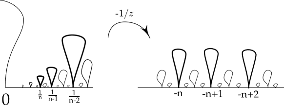
Each monotonic family of circle diffeomorphisms $f_{\omega}$ gives rise to the ‘‘fractal-like’’ set $\bigcup_{p/q\in\mathbb{Q}}B_{p/q,F_{\omega}}$ (bubbles) in $\mathbb{H}$, containing countably many analytic curves ‘‘growing’’ from rational points. These curves may intersect and self-intersect as shown in [4]; some pictures of bubbles are also presented there. The aim of this article is to prove that the bubbles of monotonic families are approximately self-similar near rational points, and to describe the ‘‘limit shapes’’ of bubbles.

1.6. Self-similarity of bubbles near zero

Let $f_{\varepsilon}$, $\varepsilon\in J$, be an analytic monotonic family of circle diffeomorphisms; here $J\subset\mathbb{R}$ is an open interval. Let $F_{\varepsilon}$ be a lift of $f_{\varepsilon}$. We consider the bubbles near zero, i.e. $B_{r,F_{\varepsilon}}$ as $r\to 0,r\in\mathbb{Q}^{+}$ (for $r<0$, the consideration is analogous). The corresponding intervals $I_{r,F_{\varepsilon}}$ accumulate to the right endpoint of $I_{0,F_{\varepsilon}}$. We assume that this right endpoint is $\varepsilon=0$ and write $f:=f_{0}$, $F:=F_{0}$.

Since $0$ is the right endpoint of $I_{0,F_{\varepsilon}}$, we have ${\mathrm{rot}\,F=0}$, $F$ has only parabolic fixed points, and we must have $F(x)\geq x$ for all $x\in\mathbb{R}$, so that the parabolic fixed points of $F$ disappear as $\varepsilon$ increases.

We impose additional genericity assumptions on $f_{\varepsilon}$. We assume that $f$ has the only parabolic fixed point, and shift it to $0$, so that $F(0)=0$, $f^{\prime}(0)=1$. We assume that this fixed point has multiplicity 2, i.e. $f^{\prime\prime}(0)\neq 0$. We also assume $\frac{\partial f}{\partial\varepsilon}(0)>0$.

In Sec. 1.8, we present the construction of a circle diffeomorhpism ${\mathbf{K}}$; in an appropriate chart, the family ${\mathbf{K}}+c$ becomes the family of Lavaurs maps for the parabolic fixed point $0$ of $F$, and $c$ is the Lavaurs phase (see Definition 17). It turns out that self-similarity patterns of bubbles of $f_{\varepsilon},\varepsilon>0$, are related to the bubbles of ${\mathbf{K}}$. The map ${\mathbf{K}}$ (‘‘transition map’’) for $C^{2}$ circle diffeomorphisms was introduced in [13] as a modulus of $C^{1}$ classification; its role in the bifurcations of parabolic points of circle diffeomorphisms was studied in [15, Theorem 6] and [14].

Put $R(z):=-1/z$. Take any rational number $p/q\in\mathbb{Q},0\leq p/q\leq 1$. Denote $a_{n}=-\frac{1}{(p/q)-n}$; then $a_{n}\to 0$ and $R(a_{n})=(p/q)-n$.

Theorem 7 (Limit shapes of bubbles-1).

Let a monotonic analytic family of circle diffeomorphisms $f_{\varepsilon}$ be as above. In the above notation, the set of limit points of the curves $R(B_{a_{n},F_{\varepsilon}})\mod 1\subset\mathbb{C}/\mathbb{Z}$ as $n\to\infty$ includes the $p/q$-bubble of the family ${\mathbf{K}}+c$.

With an additional requirement on ${\mathbf{K}}$, we get the following stronger result.

Theorem 8 (Limit shapes of bubbles-2).

In assumptions of Theorem 7, suppose that for all $c$, whenever $\mathrm{rot}\,({\mathbf{K}}+c)=p/q$, the diffeomorphism ${\mathbf{K}}+c$ has at most one parabolic cycle.

Then the curves $R(B_{a_{n},F_{\varepsilon}})\mod 1\subset\mathbb{C}/\mathbb{Z}$ (with some parametrizations) tend uniformly to the $p/q$-bubble of the family ${\mathbf{K}}+c$ as $n\to\infty$.

Figure 1. Self-similarity of bubbles. The $a_{n}$-bubbles with $a_{n}=1/n,p/q=0$, are shown in thick.

The weaker version of this theorem holds true even in assumptions of Theorem 7, see Theorem 35 below; we postpone its statement till Sec. 2.6 because it is more technical.

Remark 9.

The additional requirement in Theorem 8 (that the maps $\mathbf{K}+c$ with rotation number $p/q$ do not have two parabolic cycles simultaneously) is open and dense, see the sketch of the proof in Sec. 1.9. This condition cannot be removed. The reason for this is that the complex rotation number is not continuous at diffeomorphisms with two parabolic cycles, see Remark 46. The requirement is used in Lemma 33.

Theorem 8 implies the following self-similarity.

Theorem 10 (Self-similarity of bubbles-1).

In assumptions of Theorem 8, the set $\bigcup_{n}B_{a_{n},F_{\varepsilon}}$ is approximately self-similar near the point $0$, with the self-similarity given by $z\mapsto\frac{z}{1+z}$.

Formally, the distance in $C$ metrics between the curves $R(B_{a_{n},F_{\varepsilon}})$ and $R(B_{a_{n+1},F_{\varepsilon}})+1$ (with some parametrizations) tends to zero as $n\to\infty$.

Note that $R$ conjugates the shift $z\mapsto z-1$ to $z\mapsto\frac{z}{z+1}$, which motivates the informal statement that the self-similarity of $\bigcup_{n}B_{a_{n},F_{\varepsilon}}$ is given by $z\mapsto\frac{z}{z+1}$.

Proof.

Theorem 8 implies that the distance between $R(B_{a_{n},F_{\varepsilon}})$ and $R(B_{a_{n+1},F_{\varepsilon}})$ in $\mathbb{C}/\mathbb{Z}$ tends to zero. Recall that the map $R$ takes the sequence $\{a_{n}\}$ to $\{(p/q)-n\}$, so it takes the bubble $B_{a_{n},F_{\varepsilon}}$ to a continuous curve with both endpoints at $(p/q)-n$. Since $R(B_{a_{n},F_{\varepsilon}})$ and $R(B_{a_{n+1},F_{\varepsilon}})$ start at points $(p/q)-n$ and $(p/q)-n-1$ respectively, and are close in $\mathbb{C}/\mathbb{Z}$, the conclusion follows.

∎

Another version of a self-similarity result is the following.

Theorem 11 (Self-similarity of bubbles-2).

In assumptions of Theorem 7, suppose that ${\mathbf{K}}+c$ has at most one parabolic cycle for each $c$. Then the whole set of bubbles $\bigcup_{a,b}B_{a/b,F_{\varepsilon}}$ is approximately self-similar near $0$.

Formally, we have the following convergence of the countable unions of analytic curves:

(3) $$R\left(\bigcup_{\frac{a}{b}\in\mathbb{Q},\frac{a}{b}\in[\frac{1}{n},\frac{1}{n+1}]}B_{a/b,F_{\varepsilon}}\right)+n\to\left(\bigcup_{\frac{p}{q}\in\mathbb{Q},\frac{p}{q}\in[0,1]}B_{p/q,\mathbf{K}+c}\right)$$

as $n\to\infty$, and the convergence is uniform.

Proof.

For a small $\delta>0$, we should prove that for $n$ large, the above union is $\delta$-close to the bubbles of ${\mathbf{K}}+c$.

Clearly, any rational number $a/b>0$ sufficiently close to $0$ appears in a sequence $\{a_{n}\}$ for some appropriate $p/q$, namely $p/q=\{-b/a\}$. If in the union (3) we only take $a/b$ that correspond to finitely many $q$, the statement follows from Theorem 8. We will see that for $a/b$ corresponding to large $q$, the statement holds authomatically, which will finish the proof.

Formally, let $a/b$ be small and appear in a sequence $\{\frac{1}{(p/q)-n)}\}$: $a=q,b=p-qn$. Then due to Theorem 4 case 3, the bubble $B_{a/b,F_{\varepsilon}}$ is within the $C/b^{2}$-neighborhood of $a/b$. The direct computation shows that $R(B_{a/b,F_{\varepsilon}})$ is within the $C^{\prime}/q^{2}$-neighborhood of $p/q$. Here $C,C^{\prime}$ are constants that depend on the family $f_{\varepsilon}$ only. Thus for sufficiently large $q$, $B_{a/b,F_{\varepsilon}}$ belongs to the $\delta$-neighborhood of $B_{p/q,{\mathbf{K}}+c}$.

∎

Remark 12.

Above we mentioned (Remark 9) that for any $p/q$, the additional requirement on ${\mathbf{K}}$ in Theorem 8 corresponds to an open and dense set of $f$. Hence the additional requirement on ${\mathbf{K}}$ in Theorem 11 corresponds to a residual set of $f$.

1.7. Self-similarity of bubbles near any rational point

Analogous self-similarity results hold near any rational point of the real axis. We do not repeat remarks from the previous section; all of them apply for the theorems below as well.

Consider an analytic monotonic family of circle diffeomorphisms $f_{\varepsilon}$, $\varepsilon\in J$, and let $F_{\varepsilon}$ be a lift of $f_{\varepsilon}$. Fix a rational number $k/l$. We consider the bubbles $B_{s,F_{\varepsilon}}$ where $s\to k/l$, $s>k/l$. Again, we assume that the right endpoint of $I_{k/l,F_{\varepsilon}}$ is zero, and write $f:=f_{0}$, $F:=F_{0}$.

Then we have $\mathrm{rot}\,F=k/l$, $f$ has only parabolic cycles, and $F^{l}(x)-k\geq x$ for all $x\in\mathbb{R}$, so that the parabolic cycles of $f$ disappear as $\varepsilon$ increases.

We impose additional genericity assumptions on $f_{\varepsilon}$: we assume that $f$ has the only parabolic cycle, namely the orbit of $0$; we also assume that this cycle has multiplicity 2, i.e. $(f^{l})^{\prime}(0)=1$, $(f^{l})^{\prime\prime}(0)\neq 0$, and $\frac{\partial f^{l}_{\varepsilon}}{\partial\varepsilon}(0)>0$.

In Sec. 1.8, we present the construction of a circle diffeomorhpism $\tilde{\mathbf{K}}$ and explain its relation to Lavaurs maps of $f^{l}$.

Take $r,s\in\mathbb{Z}$ such that $0<r<l$ and $kr+ls=1$. Let $\tilde{R}(z)=\frac{rz+s}{-lz+k}$ (so that $\tilde{R}\in SL(2,\mathbb{Z})$). Given $p/q\in\mathbb{Q}$, $0\leq p/q\leq 1$, we put $\tilde{a}_{n}:=\tilde{R}^{-1}(p/q-n)$; then $\tilde{a}_{n}\to k/l$.

Theorem 13 (Limit shapes of bubbles-1).

In the above notation, the set of limit points of the curves $\tilde{R}(B_{\tilde{a}_{n},F_{\varepsilon}})\mod 1\subset\mathbb{C}/\mathbb{Z}$ as $n\to\infty$ includes the $p/q$-bubble of the family $\tilde{\mathbf{K}}+c$.

Theorem 14 (Limit shapes of bubbles-2).

In assumptions of Theorem 13, suppose that for all $c$, whenever $\mathrm{rot}\,(\tilde{\mathbf{K}}+c)=p/q$, the diffeomorphism $\tilde{\mathbf{K}}+c$ has at most one parabolic cycle.

Then the curves $\tilde{R}(B_{\tilde{a}_{n},F_{\varepsilon}})\mod 1$ (with some parametrizations) tend uniformly to the $p/q$-bubble of the family $\tilde{\mathbf{K}}+c$ as $n\to\infty$.

The proofs of the following results literally repeat the proofs of Theorems 10 and 11.

Theorem 15 (Self-similarity of bubbles-1).

In assumptions of Theorem 14, the set $\bigcup_{n}B_{\tilde{a}_{n},F_{\varepsilon}}$ is approximately self-similar near the point $k/l$, with the self-similarity given by $\tilde{R}^{-1}(\tilde{R}-1)$.

Formally, the distance in $C$ metrics between the curves $\tilde{R}(B_{\tilde{a}_{n},F_{\varepsilon}})$ and $\tilde{R}(B_{a_{n+1},F_{\varepsilon}})+1$ (with some parametrizations) tends to zero as $n\to\infty$.

Theorem 16 (Self-similarity of bubbles-2).

In assumptions of Theorem 13, suppose that $\tilde{\mathbf{K}}+c$ for all $c$ has at most one parabolic cycle. Then the whole set of bubbles $\bigcup_{a,b}B_{a/b,F_{\varepsilon}}$ is approximately self-similar near $p/q$.

Formally, the countable union of analytic curves

$$\tilde{R}\left(\bigcup_{\frac{a}{b}\in\mathbb{Q},\frac{a}{b}\in\tilde{R}^{-1}[-n,-n+1]}B_{a/b,F_{\varepsilon}}\right)+n$$

tends uniformly to the bubbles of $\tilde{\mathbf{K}}+c$ as $n\to\infty$.

1.8. The definition of ${\mathbf{K}}$, $\tilde{\mathbf{K}}$

1.8.1. Fatou coordinates

We define Fatou coordinates for a parabolic diffeomorphism $F\colon(\mathbb{C},0)\to(\mathbb{C},0)$ having a fixed point of multiplicity 2 at $0$ and such that $F(x)\geq x$. See [12] for the proofs of the statements below, and [3] for sketches.

Figure 2. Fatou coordinates

Let $\gamma^{-}$ be a small circle centered on $\mathbb{R}^{-}$ and passing through $0$. Then $F(\gamma^{-})$ does not intersect $\gamma^{-}$ (except at $0$). Let $\Pi$ be the domain between $\gamma^{-}$ and $F(\gamma^{-})$ with $0$ removed. Its quotient space by the action of $F$ is a cylinder (Ecalle cylinder) biholomorphically equivalent to $\mathbb{C}/\mathbb{Z}$. Let $\Psi^{-}\colon\Pi\to\mathbb{C}$ be the lift of this biholomorphism to $\Pi$. Then $\Psi^{-}$ conjugates $F$ to the shift $T_{1}\colon z\mapsto z+1$ and extends, via iterates of $F$, to some domain $U^{-}$. The map $\Psi^{-}$ is called the attracting Fatou coordinate of $F$.

Similarly we may construct the repelling Fatou coordinate $\Psi^{+}$ on some domain $U^{+}$; the corresponding circle $\gamma^{+}$ is in the right half-plane. The union $U^{+}\cup U^{-}$ covers the neighborhood of zero.

Both maps $\Psi^{\pm}$ are well-defined up to a shift. We will normalize them by requiring $\Psi^{-}(x)=0,\Psi^{+}(y)=0,$ for some points $x,y\in\mathbb{R},x<0<y$. If $F$ preserves the real axis, then all constructions are symmetric with respect to $z\mapsto\bar{z}$, so $\Psi^{\pm}$ preserve the real axis.

Definition 17.

Lavaurs maps for $F$ are the maps $L_{c}:=(\Psi^{+})^{-1}T_{c}\Psi^{-}$, $L_{c}\colon U^{-}\to\mathbb{C}$, for all $c\in\mathbb{C}$, where $T_{c}(z)=z+c$. The number $c$ is called the Lavaurs phase.

1.8.2. The definition of $\mathbf{K}$

In assumptions of Theorem 7, the chart $\Psi^{-}$ extends to $(-1,0)$ via iterates of $F$, and $\Psi^{+}$ extends to $(0,1)$. We normalize them by $\Psi^{-}(x)=0$ and $\Psi^{+}(x+1)=0$ for some $x\in(-1,0)$.

On the circle, the domains of definition of $\Psi^{\pm}$ coincide. This enables us to consider the transition map between Fatou coordinates. Formally, we put

$${\mathbf{K}}:=\Psi^{-}((\Psi^{+})^{-1}-1).$$

This map is defined on the whole real axis and commutes with the shift by $1$, hence defines an analytic circle diffeomorphism. This is the map we need for Theorems 7 and 8.

Another viewpoint on the same map is the following. Between the fundamental domains $[x,F(x)]$ and $[x+1,F(x+1)]$, we have two natural maps: one is the shift by $1$, the other one is a Lavaurs map. Now, $\mathbf{K}$ is their composition, in the appropriate chart. This is formalized as follows.

Remark 18.

In the chart $\Psi^{+}(z+1)=\Psi^{+}T_{1}$ on $(-1,0)$, the map ${\mathbf{K}}+c$ turns into the Lavaurs map $L_{c}-1$:

$$T_{-1}(\Psi^{+})^{-1}T_{c}\Psi^{-}((\Psi^{+})^{-1}-1)\Psi^{+}T_{1}=T_{-1}(\Psi^{+})^{-1}T_{c}\Psi^{-}=L_{c}-1.$$

1.8.3. The definition of $\tilde{\mathbf{K}}$

In assumptions of Theorem 13, the map $f^{l}$ has a parabolic fixed point of multiplicity $2$ at zero, and its orbit under $f$ consists of $l$ points. Let $a:=f^{-r}(0)$ and $b:=f^{r}(0)$ be the closest returns of this orbit to $0$, $-1<a<0<b<1$, $0<r<l$. Both $a,b$ are fixed points for $f^{l}$. Consider Fatou coordinates $\Psi^{\pm}$ of $0$ as a fixed point of $F^{l}-k$. Then $\Psi^{-}$ extends to $(a,0)$ via iterates of $F^{l}-k$, and $\Psi^{+}$ extends to $(0,b)$. We choose the normlization of $\Psi^{\pm}$ so that $\Psi^{-}(x)=0$ and $\Psi^{+}(f^{r}(x))=0$ for some $x\in(a,0)$.

Now, there are two coordinates defined on $(a,0)$, namely $\Psi^{-}$ and the Fatou coordinate of $a$ as the fixed point of $f^{l}$. The latter is the image of $\Psi^{+}$ under $f^{-r}$. We consider the transition map

$$\tilde{\mathbf{K}}:=\Psi^{-}(f^{-r}(\Psi^{+})^{-1}).$$

It is well-defined on $\mathbb{R}$ and commutes with the shift by $1$, thus defines an analytic circle diffeomorphism; this is the map we need for Theorems 13 and 14.

Another viewpoint on the same map is the following. Between the fundamental domains $[x,f^{l}(x)]\subset(a,0)$ and $f^{r}([x,f^{l}(x)])\subset(0,b)$, there are two natural maps: namely, $f^{l}$ and the Lavaurs map of $0$ for $F^{l}$. The map $\tilde{\mathcal{K}}$ in the appropriate chart is their difference. Formally, we have the following statement.

Remark 19.

In the chart $\Psi^{+}$ on $(0,b)$, the map $\tilde{\mathbf{K}}+c$ turns into

$$(\Psi^{+})^{-1}T_{c}\Psi^{-}f^{-r}(\Psi^{+})^{-1}\Psi^{+}=(\Psi^{+})^{-1}T_{c}\Psi^{-}f^{-r}=L_{c}f^{-r}$$

where $L_{c}$ is a Lavaurs map for $F^{l}$.

The above construction is a generalization of the construction from Sec. 1.8.2, with $l=1$, $r=0$.

Remark 20.

The number $r$ introduced above coincides with the number $r$ from Theorem 13. Indeed, the (periodic) orbit of $0$ under $f$ is ordered in the same way as any orbit of the translation $T_{k/l}(x)=x+k/l$, because $\mathrm{rot}\,f=k/l$. For the translation, the closest point of the orbit of $0$ to $0$ is $1/l$. So the number $r$ above satisfies $(T_{k/l})^{r}(x)=x+1/l$. This implies $kr\equiv 1\mod l$, and there exists the only integer $r,0<r<l,$ with this property. For this $r$, we have $kr-1\equiv 0\pmod{l}$, i.e. there exists an integer $s$ such that $kr+ls=1$. So this is the number $r$ from Theorem 13.

1.9. Genericity of the additional restriction on K in Theorem 8

Let $\mathbf{K}_{f}:=\mathbf{K}$ be the transition map that corresponds to the parabolic diffeomorphism $f$. Recall that the additional assumption on K in Theorem 8 was as follows:

(4) ‘‘For any $$c \mathrm{rot}\,(\mathbf{K}_{f}+c)=p/q \mathbf{K}_{f}+c$$, whenever , the map has

at most one parabolic orbit’’.

We will sketch the proof of the fact that this condition holds for a generic $f$. The same result holds true for $\tilde{\mathbf{K}}$.

Lemma 21.

For any fixed $p/q$, the set of parabolic diffeomorphisms $f$ that correspond to $\mathbf{K}_{f}$ satisfying (4) is open and dense in the metric of uniform convergence.

Sketch of the proof.

Clearly, (4) defines an open and dense set in the space of all circle diffeomorphisms. So we will focus on the map $f\mapsto\mathbf{K}_{f}$, to see that the set of corresponding $f$ is open and dense as well.

It is well-known (see [12, Proposition 2.5.2 (iii)]) that Fatou coordinates depend continuously on a (parabolic) map $F$. Thus the mapping $f\mapsto\mathbf{K}_{f}$ is continuous. Therefore the set under consideration is open.

Now it suffices to prove that we may perturb any initial circle diffeomorphism $f$ to achieve an arbitrary perturbation of $\mathbf{K}_{f}$ (i.e. that the mapping $f\mapsto\mathbf{K}_{f}$ is open). This will imply the statement.

The idea of the proof is the following: we fix the diffeomorphism $f$, cut the circle where $f$ acts, and glue again, with the gluing close to identical. This produces a new circle diffeomorphism on a ‘‘new’’ circle. In an appropriate chart on the ‘‘new’’ circle, the new diffeomorphism is close to $f$. The transition map $\mathbf{K}_{f}$ between Fatou coordinates changes in a controllable way which implies the statement.

In more detail, fix $F$ and a point $x,-1<x<0$. Consider the interval $I=[x,F(x+1)]$ with the map $F|_{[x,x+1]}$ on it. Here we ‘‘cut’’ the circle where $f$ acts: namely, $F|_{[x,x+1]}$ induces $f$ on $I/T_{1}\sim\mathbb{R}/\mathbb{Z}$. Choose another gluing: take any analytic map $h\approx T_{-1}$ that takes a neighborhood of $[x+1,F(x+1)]$ to a neighborhood of $[x,F(x)]$ and commutes with $F$; consider the quotient $I/h$ (‘‘new’’ circle). This quotient is a one-dimensional real-analytic manifold homeomorphic to a circle, thus it is a circle: there exists a real analytic map $H\colon\mathbb{R}/\mathbb{Z}\to I/h$. Its lift $\tilde{H}\colon\mathbb{R}\to I$ conjugates $h$ to the shift by $(-1)$, $H(x-1)=h(H(x))$. We will see that $H$ is close to identity.

Thus $\tilde{f}=H^{-1}fH$ is an analytic circle diffeomorphism close to $f$. Its Fatou coordinates are $\Psi^{\pm}H$, and the corresponding transition map is $\mathbf{K}_{\tilde{f}}=\Psi^{-}H(H^{-1}\Psi^{+})^{-1}-1)=\Psi^{-}(h(HH^{-1}(\Psi^{+})^{-1}))=\Psi^{-}h(\Psi^{+})^{-1}$. Since $h$ is an arbitrary map close to the shift $T_{-1}$ that commutes with $F$, we may achieve any perturbation of $\mathbf{K}_{f}$.

It remains to prove that $H$ is close to identity. The proof relies on Ahlfors-Bers theorem, and we only sketch it here. Namely, we consider a neighborhood $V$ of $I$; $V/h$ is an annulus. It is easy to find a smooth map $R_{1}$ close to $id$ in $C^{2}$, such that $R_{1}$ takes $V/h$ to a standard annulus $A$ and commutes with $z\to\bar{z}$. Now, $R_{1}$ induces a conformal structure on $A$. It is close to the standard conformal structure, hence due to Ahlfors-Bers theorem, there exists a quasiconformal map $R_{2}\approx id$ that uniformizes this conformal structure. The uniqueness of the (normalized) uniformization implies that $R_{2}$ commutes with $z\mapsto\bar{z}$. Finally, we take $H:=R_{1}^{-1}R_{2}^{-1}$, which is close to identity because both $R_{1},R_{2}$ are close to identity, and $H$ preserves the real axis because it commutes with $z\mapsto\bar{z}$. This completes the proof. ∎

1.10. Lavaurs theorem

The following theorem was proved by Lavaurs [9], see also [12, Proposition 3.2.2].

Theorem 22.

Let $F_{\varepsilon}$, $\varepsilon\in\mathbb{R}$, be an analytic family of analytic maps in a neighborhood of zero, satisfying $F_{0}(z)=z+az^{2}+\dots$, $a\neq 0$. Let $L_{c}$ be Lavaurs maps for $F_{0}$.

Suppose that $F_{\varepsilon}$ has two complex hyperbolic fixed points near zero for $\varepsilon>0$ small. Assume that both multipliers $\mu_{1,2}$ of these points satisfy $\arg|\frac{1}{2\pi i}\log\mu_{1,2}|<\pi/4$. Suppose that $\varepsilon_{k}\to 0$ and $n_{k}\to\infty$ satisfy

(5) $$\lim_{k\to\infty}F^{n_{k}}_{\varepsilon_{k}}(x)=L_{c}(x).$$

Then $F_{\varepsilon_{k}}^{n_{k}}\to L_{c}$ uniformly on compact sets in $U^{-}$.

The above assumption on multipliers for our family $F_{\varepsilon}$ follows from our genericity assumption $\frac{\partial F}{\partial\varepsilon}(0)>0$. See also [3, Propositions 13.1 and 18.2] for the particular case $F_{\varepsilon}(z)=z+z^{2}+\varepsilon$ which does not essentially differ from the general case.

2. Proof of the main theorem

2.1. Renormalizations and complex rotation numbers

It is well-known that the renormalization of a circle diffeomorphism with rotation number $\rho,0<\rho<1$, has the rotation number $-1/\rho$. It turns out that the same result holds for complex rotation numbers. First, we recall the definition of renormalization.

Take a fundamental domain $[x,g(x)]$ of an analytic circle diffeomorphism $g$ with no fixed points. The first return map to this domain under iterates of $g$ commutes with $g$, hence it descends to the quotient $[x,g(x)]/g$. Such self-map $\mathcal{R}g$ of $[x,g(x)]/g$ is called the renormalization of $g$.

Clearly, the quotient is a one-dimensional real-analytic manifold analytically equivalent to a circle. On this circle, $\mathcal{R}g$ is an analytic circle diffeomorphism. It is well-defined up to an analytic coordinate change.

There is no canonical choice of an analytic chart on the circle $[x,g(x)]/g$. However the complex rotation number does not depend on the choice of the analytic chart, due to the following lemma (for the proof, see [4, Lemma 8] or Remark 37 below).

Lemma 23.

Complex rotation number $\bar{\tau}|_{\mathbb{R}}$ is invariant under analytic conjugacies: for two analytically conjugate circle diffeomorphisms $f_{1},f_{2}$, we have $\bar{\tau}(f_{1})=\bar{\tau}(f_{2})$.

So $\bar{\tau}(\mathcal{R}g)$ is well-defined. The following lemma relates $\bar{\tau}(\mathcal{R}g)$ to $\bar{\tau}(g)$. Recall that $R(z)=-1/z$.

Lemma 24 (Complex rotation numbers under renormalizations).

Let $g$ be an analytic circle diffeomorphism with no fixed points, let $G$ be its lift to the real line with $0<\mathrm{rot}\,G<1$. Then

(6) $$\bar{\tau}(\mathcal{R}g)\equiv-\frac{1}{\bar{\tau}(G)}\equiv R(\bar{\tau}(G))\pmod{1}.$$

The proof is postponed till Sec. 4.

2.2. Renormalization at a rational point

If the rotation number of a circle diffeomorphism $g$ is close to $k/l$, it is reasonable to consider the following $k/l$-renormalization of $g$.

Suppose that $\mathrm{rot}\,g>k/l$ is sufficiently close to $k/l$. We consider the first-return map under $g$ to the segment $[x,g^{l}(x)]$. This map descends to the well-defined map $\mathcal{R}^{k/l}g$ on $[x,g^{l}(x)]/g^{l}$. Then $\mathcal{R}^{k/l}g$ is called the $k/l$-renormalization of $g$. It is induced by some powers of $g$; the following lemma gives an explicit form of the first-return map.

Lemma 25.

Let $k/l\in\mathbb{Q}$ be an irreducible fraction, and let $r$, $0<r<l$, be such that $kr\equiv 1\mod l$. Let $g$ be a circle diffeomorphism with $\mathrm{rot}\,g>k/l$ sufficiently close to $k/l$.

Then for some $n$, the first-return map on $[x,g^{l}(x)]$ under $g$ has the form $g^{nl-r}$ on $[x,a]$ and $g^{(n-1)l-r}$ on $[a,g^{l}(x)]$, where $a=g^{l(1-n)+r}(x)$.

The proof is postponed till Sec. 5.

The following lemma is an analogue of Lemma 24.

Lemma 26.

Let $g$ be a circle diffeomorphism with $\mathrm{rot}\,g>k/l$ sufficiently close to $k/l$. Let $G$ be its lift to the real line such that $\mathrm{rot}\,(G^{l}-k)\in(0,1)$. Let $r,s$ be integer numbers such that $rk+sl=1$. Then

$$\bar{\tau}(\mathcal{R}^{k/l}g)\equiv\frac{r\bar{\tau}(G)+s}{-l\bar{\tau}(G)+k}\pmod{1}.$$

Note that the above expression for $\bar{\tau}(\mathcal{R}^{k/l}g)$ equals $\tilde{R}(\bar{\tau}(G))$ where $\tilde{R}$ is defined as in Theorem 13. The proof is postponed till Sec. 4.

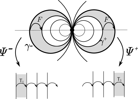
2.3. Parabolic renormalization: through the eggbeater

In this section, we will see that the renormalizations of the maps $f_{\varepsilon}$ tend to the family of Lavaurs maps $L_{c}$. This is a well-known corollary of the Lavaurs theorem, however we provide a proof due to the lack of a suitable reference. We will prove this fact in analytic charts close to $\Psi^{+}(z+1)$, and the maps $L_{c}$ will turn into the family $\mathbf{K}+c$.

This induces a reparametrization of $(0,\varepsilon)$, more or less by this $c$. We study this parametrization in Lemmas 28 and 29 of this section. Now let us pass to more details.

In assumptions of Theorem 7, recall that $\Psi^{\pm}$ are Fatou coordinates of $F$ at zero, normalized by $\Psi^{-}(x)=0$ and $\Psi^{+}(x+1)=0$, where $-1<x<0$. For each small $\varepsilon>0$, consider renormalizations $\mathcal{R}f_{\varepsilon}$, of our family $f_{\varepsilon}$, associated with fundamental domains $[x,F_{\varepsilon}(x)]$. Each map $\mathcal{R}f_{\varepsilon}$ acts on its own circle $[x,F_{\varepsilon}(x)]/F_{\varepsilon}$.

For each small $\varepsilon>0$, put $d(\varepsilon):=\Psi^{+}F^{n}_{\varepsilon}(x)$, where $n=n(\varepsilon)$ is the smallest integer number such that $F^{n}_{\varepsilon}(x)\in[x+1,F_{\varepsilon}(x)+1]$.

Consider analytic charts $\chi_{\varepsilon}\colon[x,F_{\varepsilon}(x)]/F_{\varepsilon}\to\mathbb{R}/\mathbb{Z}$ that converge to the chart $(\Psi^{+}(z+1)\mod 1)$ on $[x,F(x)]/F$ as $\varepsilon\to 0$; the convergence is uniform in a neighborhood of $[x,F_{\varepsilon}(x)]$ in $\mathbb{C}$. For example, we may take perturbed Fatou coordinates of $F_{\varepsilon}$, see [12, Proposition 3.2.2, coordinates $\Phi_{\pm,f}$].

Lemma 27.

Under assumptions of Theorem 7, suppose that the sequence $\varepsilon_{k}\to 0$, $\varepsilon_{k}>0$, satisfies $d(\varepsilon_{k})\to c$. Then $\chi_{\varepsilon}(\mathcal{R}f_{\varepsilon})\chi_{\varepsilon}^{-1}$ tends to ${\mathbf{K}}+c$ as $k\to\infty$, uniformly on some neighborhood of $\mathbb{R}/\mathbb{Z}$ in $\mathbb{C}/\mathbb{Z}$.

Proof.

The definition of $\mathcal{R}f_{\varepsilon}$ suggests that we study the maps $F_{\varepsilon_{k}}^{n(\varepsilon_{k})}-1$ and $F_{\varepsilon_{k}}^{n(\varepsilon_{k})-1}-1$ on $[x,F_{\varepsilon}(x)]$.

Since $d(\varepsilon_{k})\to c$, we have that

(7) $$\lim_{k\to\infty}F_{\varepsilon_{k}}^{n(\varepsilon_{k})}(x)=(\Psi^{+})^{-1}(c).$$

Note that $L_{c}(x)=(\Psi^{+})^{-1}T_{c}\Psi^{-}(x)=(\Psi^{+})^{-1}(c)$ due to our normalization $\Psi^{-}(x)=0$, so the right-hand side of (7) equals $L_{c}(x)$. Due to Lavaurs theorem (Theorem 22), in some neighborhood of $[x,F_{\varepsilon}(x)]$ in $\mathbb{C}$, the maps $F^{n(\varepsilon_{k})}_{\varepsilon_{k}}$ tend uniformly to the Lavaurs map $L_{c}$. So the maps $F^{n(\varepsilon_{k})}_{\varepsilon_{k}}-1$ converge uniformly to $L_{c}-1$ in some neighborhood of $[x,F_{\varepsilon}(x)]$, and the maps $F^{n(\varepsilon_{k})-1}_{\varepsilon_{k}}-1$ converge uniformly to $L_{c-1}-1=F^{-1}L_{c}-1$. Due to Remark 18, in the chart $\Psi^{+}(z+1)$ on $[x,F(x)]$, the map $L_{c}-1$ equals ${\mathbf{K}}+c$. So in the chart $(\Psi^{+}(z+1)\mod 1)$ on $[x,F(x)]/F$, the maps $L_{c}-1$ and $L_{c-1}-1$ equal ${\mathbf{K}}+c$. Therefore, in any analytic charts on $[x,F_{\varepsilon}(x)]/F_{\varepsilon}$ that tend to $(\Psi^{+}(z+1)\mod 1)$, we have the following uniform convergence in a neighborhood of $\mathbb{R}/\mathbb{Z}$:

$$\chi_{\varepsilon}(F_{\varepsilon_{k}}^{n(\varepsilon_{k})}-1)\chi_{\varepsilon}^{-1}\to{\mathbf{K}}+c$$

$$\chi_{\varepsilon}(F_{\varepsilon_{k}}^{n(\varepsilon_{k})-1}-1)\chi_{\varepsilon}^{-1}\to{\mathbf{K}}+c.$$

Since $\mathcal{R}f_{\varepsilon}$ is induced by $F_{\varepsilon_{k}}^{n(\varepsilon_{k})}-1$ on the one subsegment of $[x,F_{\varepsilon}(x)]/F_{\varepsilon}$ and by $F_{\varepsilon_{k}}^{n(\varepsilon_{k})-1}-1$ on the other, the result follows.

∎

The function $d(\cdot)$ defined above is almost suitable as a parametrization of bubbles $B_{a_{n},F_{\varepsilon}}$ needed for Theorem 8. The following two lemmas study this function.

Lemma 28.

The function $d(\cdot)$ is monotonic and continuous on $I_{r,F_{\varepsilon}}$ if $r\neq 1/n$. On $I_{1/n,F_{\varepsilon}}$ it is monotonic whenever continuous and has a jump. The size of the jump tends to $1$ from above as $n\to\infty$. In any case, the values of $d(\varepsilon)$ for $\varepsilon$ small belong to a small neighbohood of $[0,1]$.

Proof.

The last claim is clear because $\Psi^{+}([x+1,F_{\varepsilon}(x)+1])$ is close to $\Psi^{+}([x+1,F(x)+1])=[0,1]$.

Since $F^{n}_{\varepsilon}$ is monotonic, the function $d(\cdot)$ is monotonic whenever continuous. It has jumps at the points $\varepsilon_{n}$ with $F^{n}_{\varepsilon_{n}}(x)=x+1$, i.e. where $\mathcal{R}f_{\varepsilon_{n}}(x)=x$. So the jump points belong to the set $\{\mathrm{rot}\,\mathcal{R}f_{\varepsilon}=0\}$, i.e. to $I_{1/n,F_{\varepsilon}}$.

The size of the jump is $\Psi^{+}F_{\varepsilon_{n}}(x)-\Psi^{+}(x)$, which tends to $\Psi^{+}F(x)-\Psi^{+}(x)=1$ from above as $\varepsilon_{n}\to 0$. ∎

Recall that $a_{n}=-1/(p/q-n)$, as in Theorem 7. The following lemma shows that $d(\cdot)$ takes the segments $I_{a_{n},F_{\varepsilon}}$ that parametrize bubbles $B_{a_{n},F_{\varepsilon}}$ (approximately) to the segments $I_{p/q,\mathbf{K}+\omega}$ that parametrize $B_{p/q,\mathbf{K}+\omega}$.

Lemma 29.

Put $I_{n}:=d(I_{a_{n},F_{\varepsilon}})\mod 1\subset\mathbb{R}/\mathbb{Z}$. Then the set of limit points of $I_{n}$ as $n\to\infty$ coincides with $I_{p/q,{\mathbf{K}}+\omega}\mod 1$.

Proof.

Let $d$ be a limit point of $I_{n}$, and let us prove that $d\in I_{p/q,{\mathbf{K}}+\omega}$. Take $\varepsilon_{k}\in I_{a_{n_{k}},F_{\varepsilon}}$ such that $d(\varepsilon_{k})\to d$; then due to Lemma 27, $\chi_{\varepsilon_{k}}(\mathcal{R}f_{\varepsilon_{k}})\chi_{\varepsilon_{k}}^{-1}\to{\mathbf{K}}+d$. Note that $\mathrm{rot}\,\chi_{\varepsilon_{k}}(\mathcal{R}f_{\varepsilon_{k}})\chi_{\varepsilon_{k}}^{-1}=\mathrm{rot}\,\mathcal{R}f_{\varepsilon}=-1/\mathrm{rot}\,F_{\varepsilon}$, so for $\varepsilon_{k}\in I_{a_{n_{k}},f_{\varepsilon}}$, we have $\mathrm{rot}\,\chi_{\varepsilon_{k}}(\mathcal{R}f_{\varepsilon_{k}})\chi_{\varepsilon_{k}}^{-1}\equiv-1/a_{n_{k}}\equiv p/q\pmod{1}$. This implies $\mathrm{rot}\,({\mathbf{K}}+d)=p/q$, hence $d\in I_{p/q,{\mathbf{K}}+\omega}$.

If $I_{p/q,{\mathbf{K}}+\omega}$ is just one point, the proof is finished. If $I_{p/q,{\mathbf{K}}+\omega}$ is a segment, we also need to prove that any point of $I_{p/q,{\mathbf{K}}+\omega}$ is a limit point of $I_{n}$. Take $c\in I_{p/q,{\mathbf{K}}+\omega}$ such that ${\mathbf{K}}+c$ is hyperbolic. This holds for all points of $I_{p/q,{\mathbf{K}}+\omega}$ except a finite set. Let $\varepsilon_{k}\to 0$ be such that $d(\varepsilon_{k})\equiv c\pmod{1}$; the existence of such an infinite sequence $\varepsilon_{k}$ follows from the definition of $d$. Then $\chi_{\varepsilon_{k}}(\mathcal{R}f_{\varepsilon_{k}})\chi_{\varepsilon_{k}}^{-1}$ tends to the hyperbolic map ${\mathbf{K}}+c$ due to Lemma 27, so $\mathrm{rot}\,(\chi_{\varepsilon_{k}}(\mathcal{R}f_{\varepsilon_{k}})\chi_{\varepsilon_{k}}^{-1})=p/q$ for large $k$. This implies $\varepsilon_{k}\in\bigcup I_{a_{n},F_{\varepsilon}}$ as explained above. Finally, $c$ belongs to the set of limit points of $I_{n}$.

Since the set of limit points is closed, $I_{p/q,{\mathbf{K}}+\omega}$ belongs to the set of limit points of $I_{n}$.

∎

2.4. Parabolic renormalization at a rational point

Here we prove the analogues of the results from the previous section for the case $\mathrm{rot}\,f=k/l$.

Let $f$ be a circle diffeomorphism having one parabolic cycle of period $l$, $f^{l}(0)=0$. The analogue of Lemma 27 is the following. Recall that we normalize Fatou coordinates of $f^{l}$ at $0$ by $\Psi^{-}(x)=0$, $\Psi^{+}(y)=0$ where $x\in(a,0),y:=f^{r}(x)\in(0,b)$. For each small $\varepsilon>0$, put $\tilde{d}(\varepsilon):=\Psi^{+}f^{nl}_{\varepsilon}(x)$, where $n=n(\varepsilon)$ is the smallest number such that $f^{nl-r}_{\varepsilon}(y)=f^{nl}_{\varepsilon}(x)\in[y,f_{\varepsilon}^{l}(y)]$. Due to Lemma 39, this is the first point of the orbit of $y$ that belongs to $[y,f_{\varepsilon}^{l}(y)]$. Let $\mathcal{R}^{k/l}f_{\varepsilon}$ be $k/l$-renirmalizations associated with fundamental domains $[y,f^{l}_{\varepsilon}(y)]$.

Note that $(\Psi^{+}\mod 1)$ defines an analytic chart on $[y,f^{l}(y)]/f^{l}$. Consider analytic charts $\tilde{\chi}_{\varepsilon}$ on the circles $[y,f^{l}_{\varepsilon}(y)]/f^{l}_{\varepsilon}$ that converge to the chart $(\Psi^{+}\mod 1)$ on $[y,f^{l}(y)]/f^{l}$, and the convergence is uniform on some neighborhood of $[y,f^{l}(y)]$ in $\mathbb{C}$. Again, we may take perturbed Fatou coordinates of $f_{\varepsilon}^{l}$.

Lemma 30.

Under assumptions of Theorem 13, suppose that the sequence $\varepsilon_{k}\to 0,\varepsilon_{k}>0$, is such that $\tilde{d}(\varepsilon_{k})\to c$. Then $\tilde{\chi}_{\varepsilon}(\mathcal{R}^{k/l}f_{\varepsilon})\tilde{\chi}_{\varepsilon}^{-1}$ tends to $\tilde{\mathbf{K}}+c$ as $k\to\infty$, uniformly on some neighborhood of $\mathbb{R}/\mathbb{Z}$ in $\mathbb{C}/\mathbb{Z}$.

Proof.

Since $d(\varepsilon_{k})\to c$, we have that $f_{\varepsilon_{k}}^{ln(\varepsilon_{k})}(x)$ tends to $(\Psi^{+})^{-1}(c)$, which equals $L_{c}(x)$, where $L_{c}=(\Psi^{+})^{-1}T_{c}(\Psi^{-})$ is a Lavaurs map. Due to Lavaurs theorem (see Theorem 22), in some neighborhood of $[x,f^{l}_{\varepsilon}(x)]$ in $\mathbb{C}$, the maps $f^{ln(\varepsilon_{k})}_{\varepsilon_{k}}$ tend uniformly to the Lavaurs map $L_{c}$.

So $f^{ln-r}_{\varepsilon_{k}}$ on some neighborhood of $[y,f^{l}(y)]$ converge uniformly to $L_{c}f^{-r}$. Similarly, the maps $f^{l(n-1)-r}_{\varepsilon_{k}}$ converge uniformly to $L_{c-1}f^{-r}$. Due to Remark 19, in the chart $(\Psi^{+}\mod 1)$ on $[y,f^{l}(y)]/f^{l}$, the map $L_{c}f^{-r}$ equals $\tilde{\mathbf{K}}+c$. So in any analytic charts $\tilde{\chi}_{\varepsilon}$ on $[y,f_{\varepsilon}^{l}(y)]/f_{\varepsilon}^{l}$ that tend uniformly to $(\Psi^{+}(z)\mod 1)$, we have the uniform convergence $\tilde{\chi}_{\varepsilon}f_{\varepsilon_{k}}^{ln(\varepsilon_{k})-r}\tilde{\chi}_{\varepsilon}^{-1}\to\tilde{\mathbf{K}}+c$ and $\tilde{\chi}_{\varepsilon}f_{\varepsilon_{k}}^{l(n(\varepsilon_{k})-1)-r}\tilde{\chi}_{\varepsilon}^{-1}\to\tilde{\mathbf{K}}+c$. Due to Lemma 25, the map $\mathcal{R}^{k/l}(f_{\varepsilon})$ is induced by $f_{\varepsilon_{k}}^{ln(\varepsilon_{k})-r}$ on the one subsegment of $[y,f_{\varepsilon}^{l}(y)]$ and by $f_{\varepsilon_{k}}^{l(n(\varepsilon_{k})-1)-r}$ on the other, and the result follows.

∎

In the next two lemmas, we study the function $\tilde{d}(\cdot)$. We will use this function to reparametrize bubbles for Theorem 14. Recall that $r,s$ are such that $kr+ls=1$. Recall that $\tilde{R}(z)=(rz+s)/(-lz+k)$, and this is the mapping that acts on rotation numbers when we make $k/l$-renormalizations.

Lemma 31.

The function $\tilde{d}(\cdot)$ is monotonic and continuous on $I_{r,F_{\varepsilon}}$ if $\tilde{R}(r)\neq 0\pmod{1}$. Otherwise, it is monotonic whenever continuous on $I_{r,F_{\varepsilon}}$ and has a jump. The size of the jump tends to $1$ from above as $n\to\infty$. In any case, the values of $\tilde{d}(\varepsilon)$ for $\varepsilon$ small belong to a small neighborhood of $[0,1]$.

Proof.

Note that the jump of $\tilde{d}$ occurs when $f^{nl}_{\varepsilon}(x)=f^{r}_{\varepsilon}(x)$, i.e. $\mathcal{R}^{k/l}f_{\varepsilon}$ has a fixed point at $x$. This happens when $\mathrm{rot}\,\mathcal{R}^{k/l}f_{\varepsilon}=0$, i.e. $\tilde{R}(\mathrm{rot}\,f_{\varepsilon})=0$. The rest of the proof repeats the proof of Lemma 28. ∎

Recall that $p/q$ is a rational number, and the sequence $\{a_{n}\}$ is such that $\tilde{R}(a_{n})=p/q-n$.

Lemma 32.

Put $\tilde{I}_{n}:=\tilde{d}(I_{\tilde{a}_{n},F_{\varepsilon}})\mod 1\subset\mathbb{R}/\mathbb{Z}$. Then the set of limit points of $\tilde{I}_{n}$ as $n\to\infty$ coincides with $I_{p/q,\tilde{\mathbf{K}}+\omega}\mod 1$.

The proof is completely analogous to the proof of Lemma 29.

2.5. Continuity of complex rotation numbers

The following lemma shows that $\bar{\tau}$ is continuous in the metric of uniform convergence at a circle diffeomorphism with at most one parabolic cycle.

Lemma 33.

Let $g_{k}$ be a sequence of analytic circle diffeomorphisms that converges to an analytic circle diffeomorphism $g$, uniformly on some neighborhood of $\mathbb{R}/\mathbb{Z}$ in $\mathbb{C}/\mathbb{Z}$. Suppose that $g$ has at most one parabolic cycle. Then $\bar{\tau}(g_{k})\to\bar{\tau}(g)$.

The proof of this lemma constitutes Sec. 6.

2.6. Proof of Theorems 7 and 8 modulo auxiliary lemmas

The most essential components of the proofs of Theorems 7 and 8 are: the behaviour of complex rotation numbers under renormalizations (Lemma 24), the convergence of renormalizations to $\mathbf{K}+c$ (Lemma 27), and the continuity of complex rotation numbers (Lemma 33). Their proofs are contained in Sections 4, 2.3, and 6 respectively. The proofs in this section are straightforward and show how to reduce the theorems to the lemmas mentioned above.

The following lemma is a common part of the proofs of Theorems 7 and 8. We recall that $R(z)=-1/z$ and $d(\cdot)$ is defined in Sec. 2.3.

Lemma 34.

Suppose that $c\in I_{p/q,\mathbf{K}+\omega}$ and $\mathbf{K}+c$ has at most one parabolic fixed point. Let $\varepsilon_{k}\to 0$ be such that $(d(\varepsilon_{k})\mod 1)\to c$.

Then $R(\bar{\tau}(F_{\varepsilon_{k}}))\to\bar{\tau}(\mathbf{K}+c)$ in $\overline{\mathbb{H}}/\mathbb{Z}$.

Proof.

When we make renormalizations, we apply the map $R(z)=-1/z$ to complex rotation numbers (Lemma 24):

(8) $$R(\bar{\tau}(F_{\varepsilon}))\equiv\bar{\tau}(\mathcal{R}f_{\varepsilon})\pmod{1}.$$

The renormalizations $\mathcal{R}f_{\varepsilon}$ in suitable charts are close to the family $\mathbf{K}+\omega$ due to Lemma 27. Formally, take the charts $\chi_{\varepsilon}$ as in Lemma 27. Since the complex rotation number does not depend on the charts (Lemma 23), we have

(9) $$\bar{\tau}(\mathcal{R}f_{\varepsilon})=\bar{\tau}(\chi_{\varepsilon}(\mathcal{R}f_{\varepsilon})\chi_{\varepsilon}^{-1}).$$

Due to Lemma 27, the maps $\chi_{\varepsilon_{n}}(\mathcal{R}f_{\varepsilon_{n}})\chi_{\varepsilon_{n}}^{-1}$ tend to $\mathbf{K}+c$ uniformly on some neighborhood of $\mathbb{R}/\mathbb{Z}$ in $\mathbb{C}/\mathbb{Z}$. Using (8), (9), and the continuity of $\bar{\tau}$ at $\mathbf{K}+c$ (Lemma 33), we get $R(\bar{\tau}(F_{\varepsilon_{n}}))=\bar{\tau}(\chi_{\varepsilon_{n}}(\mathcal{R}f_{\varepsilon_{n}})\chi_{\varepsilon_{n}}^{-1})\to\bar{\tau}(\mathbf{K}+c)$. ∎

Proof of Theorem 7.

Recall that we consider $a_{n}$-bubbles of $F_{\varepsilon}$, $B_{a_{n},F_{\varepsilon}}$, and the map $R(z)=-1/z$ takes the sequence $\{a_{n}\}$ to the sequence $\{p/q-n\}$.

First, prove that the set of limit points of $R(B_{a_{k},F_{\varepsilon}})$ contains $B_{p/q,\mathbf{K}+\omega}\smallsetminus\mathbb{R}$.

Consider any $c\in I_{p/q,\mathbf{K}+\omega}$ such that ${\mathbf{K}}+c$ is hyperbolic; this corresponds to an arbitrary point of $B_{p/q,\mathbf{K}+\omega}\smallsetminus\mathbb{R}$. Recall that the limit points of the sequence of segments $d(I_{a_{n},F_{\varepsilon}})$ form the segment $I_{p/q,\mathbf{K}+\omega}$ (Lemma 29), so we may fix $\varepsilon_{n}\to 0,\varepsilon_{n}\in\bigcup I_{a_{k},F_{\varepsilon}}$, such that $d(\varepsilon_{n})\to c$. Due to Lemma 34, we have that $R(\bar{\tau}(f_{\varepsilon_{n}}))\to\bar{\tau}(\mathbf{K}+c)$.

So the set of limit points of $R(B_{a_{k},F_{\varepsilon}})$ contains $B_{p/q,\mathbf{K}+\omega}\smallsetminus\mathbb{R}$.

Since the set of limit points is closed, it contains $B_{p/q,{\mathbf{K}}+\omega}$ as well.

∎

Proof of Theorem 8..

In this theorem, we must present suitable parametrizations of bubbles $B_{a_{n},F_{\varepsilon}}$.

First, consider the case $p/q\neq 0$, i.e. $a_{n}$ is not the sequence $1/n$; in this case, the suitable parametrization will be the function $d(\cdot)$ introduced in Sec. 2.3. Due to Lemma 28, $d(\cdot)$ is a continuous monotonic function on $I_{a_{n},F_{\varepsilon}}$.

Suppose that the curves $R(B_{a_{n},F_{\varepsilon}})$ parametrized by $d(\cdot)$ do not tend uniformly to $B_{p/q,\mathbf{K}+c}$ parametrized by $c$. So for some $\delta>0$, there exists a sequence $\varepsilon_{k}\to 0,\varepsilon_{k}\in\bigcup I_{a_{n},F_{\varepsilon}}$, such that

(10) $$\operatorname{dist}(R(\bar{\tau}(f_{\varepsilon_{k}})),\bar{\tau}(\mathbf{K}+d(\varepsilon_{k})))>\delta.$$

Extracting subsequences, we may assume that $d(\varepsilon_{k})$ converges to some $c$. Recall that the limit points of the segments $d(I_{a_{n},F_{\varepsilon}})$ form the segment $I_{p/q,\mathbf{K}+\omega}$ (Lemma 29), hence $c\in I_{p/q,\mathbf{K}+\omega}.$

Now Lemma 34 implies that $R(\bar{\tau}(f_{\varepsilon_{k}}))\to\bar{\tau}(\mathbf{K}+c)$. Since $\bar{\tau}(\mathbf{K}+c)$ is continuous with respect to $c$, the distance in (10) must tend to zero, and we get a contradiction.

The contradiction shows that the curves $R(B_{a_{k},F_{\varepsilon}})$, parametrized by $d(\cdot)$, tend uniformly to $B_{p/q,\mathbf{K}+\omega}$, q.e.d.

If $p/q=0$, i.e. $a_{n}=1/n$, the function $d(\cdot)$ is not continuous on $I_{a_{n},F_{\varepsilon}}$. It has a jump on each segment $I_{1/n,F_{\varepsilon}}$. However the size of the jump of $(d(\cdot)\mod 1)$ tends to zero as $n\to\infty$, see Lemma 28. So there exists a continuous monotonic reparametrization $D(\cdot)\colon I_{1/n,F_{\varepsilon}}\to\mathbb{R}$ of the curves $R(B_{a_{n},F_{\varepsilon}})$ such that $(D(\varepsilon)-d(\varepsilon))\mod 1\to 0$ as $\varepsilon\to 0$. Then for any sequence $\varepsilon_{k}\to 0$, we have $d(\varepsilon_{k})\to c$ on $\mathbb{R}/\mathbb{Z}$ iff $D(\varepsilon_{k})\to c$. So Lemma 34 holds true for $D(\cdot)$. The same arguments as above imply the statement of Theorem 8. ∎

Exactly the same arguments lead to the following statement. It seems to be the strongest possible statement in assumptions of Theorem 7 only.

Theorem 35.

In assumptions of Theorem 7, let $Z$ be a finite set of values $c\in I_{p/q,\mathbf{K}+\omega}$ such that $\mathbf{K}+c$ has at least two parabolic fixed points. Let $U$ be an arbitrarily small neighborhood of $Z$. Then the curves $\{R(\bar{\tau}(f_{\varepsilon}))\mid\varepsilon\in I_{a_{n},F_{\omega}}\smallsetminus d^{-1}(U)\}$, parametrized by $d(\cdot)$ or $D(\cdot)$ as in Theorem 8, tend uniformly to $\{\bar{\tau}(\textbf{K}+c)\mid c\in I_{p/q,\mathbf{K}+\omega}\smallsetminus U\}$.

2.7. Proof of Theorems 13 and 14 modulo auxiliary lemmas

The proofs are completely analogous. We should make the following replacements:

• $\tilde{d}(\cdot)$ replaces $d(\cdot)$, $\tilde{R}$ replaces $R$, $\tilde{\mathbf{K}}$ replaces $\mathbf{K}$, $\mathcal{R}^{k/l}$ replaces $\mathcal{R}$, $\tilde{a}_{n}$ replaces $a_{n}$.

• Instead of Lemmas 24, 27, 28, and 29, we should use their direct analogues Lemmas 26, 30, 31, and 32. Their proofs are contained in Sec.4 and 2.4.

• In the proof of Theorem 14, the exceptional sequence $\{\tilde{a}_{n}\}$ is $\tilde{R}^{-1}(\mathbb{Z})$ instead of $\{1/n\}$.

All the rest of the proofs is literally the same.

3. Complex rotation numbers for hyperbolic diffeomorphisms

Let $g$ be a hyperbolic analytic circle diffeomorphism, let $G$ be its lift to the real line. In this section, we present more explicit construction of a complex rotation number $\bar{\tau}(G)$. Namely, we will construct a non-degenerate torus $\mathcal{E}(g)$ with modulus $\bar{\tau}(G)$. The construction was suggested by X.Buff and used in [5], [2].

Informally, we construct a special fundamental domain of $g$ and let $\mathcal{E}(g)$ be the quotient of this domain by the action of $g$. This fundamental domain is an annulus in $\mathbb{C}/\mathbb{Z}$ with curvilinear boundaries, it is close to $\mathbb{R}/\mathbb{Z}$ and passes above repelling cycles and below attracting cycles of $g$.

Figure 3. Construction of $\mathcal{E}(g)$ and its generators for the circle diffeomorphism $g$ with two 2-periodic hyperbolic orbits

In more detail, suppose that $g\colon\mathbb{R}/\mathbb{Z}\to\mathbb{R}/\mathbb{Z}$ has rational rotation number $p/q$ and is hyperbolic. Let $m\geq 1$ be the number of attracting cycles of $g$; it is equal to the number of repelling cycles. Let $\alpha_{j}$, $j\in\mathbb{Z}/(2mq)\mathbb{Z}$, be the periodic points of $g$, ordered cyclically; even indices correspond to attracting periodic points and odd indices to repelling periodic points. Then $g(\alpha_{j})=\alpha_{j+pm}$.

Let $\rho_{j}:=(g^{\circ q})^{\prime}(\alpha_{j})$. Let $\phi_{j}\colon(\mathbb{C},0)\to(\mathbb{C}/\mathbb{Z},\alpha_{j})$ be the uniformizing chart for $g^{\circ q}$, i.e. $g^{\circ q}\circ\phi_{j}(z)=\phi_{j}(\rho_{j}z)$, and normalize the charts so that $\phi^{\prime}_{j}(0)=1$. Then $\phi_{j}$ extends univalently to a neighborhood of the real axis, and its range contains a neighborhood of $(\alpha_{j-1},\alpha_{j+1}).$

For each $j\in\mathbb{Z}/(2mq)\mathbb{Z}$, let $x_{j}$ be a point in $(\alpha_{j},\alpha_{j+1})$. Let $C_{j}$ be an arc of a circle with endpoints $\phi_{j}^{-1}(x_{j-1})$, $\phi_{j}^{-1}(x_{j})$, such that $C_{j}$ is close to the real axis and located above $\mathbb{R}$ for odd $j$ and below $\mathbb{R}$ for even $j$. Put $\gamma=\bigcup\phi_{j}(C_{j})$. We choose $x_{j},C_{j}$ so that $g(\gamma)$ is above $\gamma$ in $\mathbb{C}/\mathbb{Z}$. This requires achieving $g(x_{j})\in(\alpha_{j+pm},x_{j+pm})$ for attracting $\alpha_{j}$ and $g(x_{j})\in(x_{j+pm},\alpha_{j+pm+1})$ for repelling $\alpha_{j}$, and the same for the heights of $C_{j}$. See [2, Sec. 5] for more details.

Then, $\gamma$ is a simple closed curve in $\mathbb{C}/\mathbb{Z}$, $g$ is univalent in a neighborhood of $\gamma$, and $g(\gamma)$ lies above $\gamma$ in $\mathbb{C}/\mathbb{Z}$; see Fig. 3. The curves $\gamma$ and $g(\gamma)$ bound the annulus $\Pi\subset\mathbb{C}/\mathbb{Z}$. Glueing its two sides via $g$, we obtain the complex torus $\mathcal{E}(g)$.

If the lift $G$ of $g$ is fixed, this torus has two distinguished generators of the first homology group: the first generator is $\gamma$, and the second one is a curve that joins $x$ to $G(x)$ in the lift of $\Pi\subset\mathbb{C}/\mathbb{Z}$ to $\mathbb{C}$, see Fig. 3. The modulus of $\mathcal{E}(g)$ is a unique $\tau=\tau(\mathcal{E}(g))\in\mathbb{H}$ such that $\mathcal{E}(g)$ is biholomorphically equivalent to $\mathbb{C}/(\mathbb{Z}+\tau\mathbb{Z})$ with its first generator corresponding to $\mathbb{R}/\mathbb{Z}$ and the second generator corresponding to $\tau\mathbb{R}/\tau\mathbb{Z}$. The modulus of $\mathcal{E}(g)$ depends on the choice of a lift $G$ in the same way as described in Sec. 1.2.

The following theorem is contained in [2].

Theorem 36.

For each hyperbolic circle diffeomoprhism $g+\omega$, the modulus $\tau(\mathcal{E}(g+\omega))$ equals the complex rotation number $\bar{\tau}_{G}(\omega)$.

Actually, the construction of $\mathcal{E}(g+\omega)$ was used as a definition of $\bar{\tau}_{g}(\omega)$ in [2, Sec. 5], so this theorem follows from the result of [2].

Remark 37.

Since $\bar{\tau}_{g}(\omega)$ equals the modulus of $\mathcal{E}(g+\omega)$, it only depends on $g+\omega$, which motivates our notation $\bar{\tau}(g+\omega)=\tau_{g}(\omega)$.

Moreover, $\mathcal{E}(g)$ does not depend on the analytic chart on the circle. Thus for two analytically conjugate diffeomorphisms $g_{1},g_{2}$, we have $\mathcal{E}(g_{1})=\mathcal{E}(g_{2})$, which implies Lemma 23.

Remark 38.

Due to [11, Sec. 2.1, Proposition 2], the modulus $\tau$ of $\mathcal{E}(g)$ depends holomorphically on $g$.

4. Complex rotation numbers under renormalizations.

Here we prove Lemmas 24 and 26.

The proof of Lemma 24.

If $\mathrm{rot}\,g$ is irrational, then $\bar{\tau}(g)=\mathrm{rot}\,g$ due to Theorem 3. Since $\mathrm{rot}\,(\mathcal{R}g)\equiv\frac{-1}{\mathrm{rot}\,g}\pmod{1}$, the number $\mathrm{rot}\,(\mathcal{R}g)$ is also irrational, and

(11) $$\bar{\tau}(\mathcal{R}g)=\mathrm{rot}\,(\mathcal{R}g)=\frac{-1}{\mathrm{rot}\,(G)}=\frac{-1}{\bar{\tau}(G)}$$

q.e.d. Similarly, if $g$ has a parabolic cycle, then so does $\mathcal{R}g$, and we have (11) again. The only remaining case is the case of a hyperbolic $g$.

Take any point $x$ that is not a periodic point of $g$. Fix $n\in\mathbb{N}$ such that the first return map to $[x,g(x)]$ under iterates of $g$ is $g^{n}$ on the one subseqment of $[x,g(x)]$ and $g^{n-1}$ on the other.

Consider the complex torus $\mathcal{E}(g)=\Pi/g$ defined in the previous section; recall that $\Pi$ is the curvilinear annulus between $\gamma$ and $g(\gamma)$. Clearly, we may assume that $\gamma$ passes through $x$, and take $\gamma$ sufficiently close to $\mathbb{R}/\mathbb{Z}$ such that $g^{n}$ is defined and univalent in the wider annulus between $\gamma$ and $g^{n+1}(\gamma)$. Let this annulus be $\Pi^{(n+1)}$. Let the lifts of the annuli $\Pi,\Pi^{(n+1)}$ to $\mathbb{C}$ be denoted by $\tilde{\Pi},\tilde{\Pi}^{(n+1)}.$

Put $\tau:=\bar{\tau}(G)$ for shortness. Due to Theorem 36, $\mathcal{E}(g)$ is biholomorphic to $\mathbb{C}/\mathbb{Z}+\tau\mathbb{Z}$. The biholomorphism $H\colon\mathcal{E}(g)\to\mathbb{C}/\mathbb{Z}+\tau\mathbb{Z}$ lifts to the map $\hat{H}\colon\tilde{\Pi}\to\mathbb{C}$ that conjugates $G$ to $z\mapsto z+\tau$ and the shift by $1$ to itself. It extends, via iterates of $G$, to the strip $\tilde{\Pi}^{(n+1)}$. Now $\hat{H}\colon\tilde{\Pi}^{(n+1)}\to\mathbb{C}$ conjugates $G$ to the shift by $\tau$. Below we show that the same map $\hat{H}$ rectifies the complex torus $\mathcal{E}(\mathcal{R}g)$.

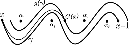
First of all, introduce a suitable construction of $\mathcal{E}(\mathcal{R}g)$; this will be a particular case of the general construction from Sec. 3.

Figure 4. Construction of $\mathcal{E}(\mathcal{R}g)$ for $g$ having two $2$-periodic orbits. The curves $\gamma,g(\gamma),g^{2}(\gamma)$ are thick, the curves $\gamma^{\prime}$ and $g^{2}(\gamma^{\prime})$ are dotted, $V$ is shadowed

Take a small neighborhood $V$ of $[x,G(x)]$ in which $G$ is univalent. Let a curve $\gamma^{\prime}\subset V$ be the union of arcs of circles in the linearizing charts of the periodic orbits of $g$, as in Sec. 3; we take one arc for each periodic point in $[x,G(x)]$, arcs are below attracting periodic points and above repelling periodic points. We assume that $\gamma^{\prime}$ satisfies the following additional requirements (see Fig. 4):

1. $\gamma^{\prime}$ joins $x$ to $G(x)$;

2. $\gamma^{\prime}$ is located between $\gamma$ and $g(\gamma)$ in $\mathbb{C}/\mathbb{Z}$.

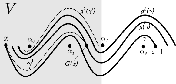
Then $\tilde{\gamma}:=\gamma^{\prime}/G$ is a closed curve in $V/G$. Moreover, $\tilde{\gamma}$ can play the role of $\gamma$ in the construction of $\mathcal{E}(\mathcal{R}g)$, see Sec. 3. Indeed, $\mathcal{R}g$ is induced by the maps $G^{n-1}-1,G^{n}-1$ on the quotient $V/G$, so has the same periodic points and linearizing charts as $G$; to satisfy the additional requirements above, we just need a suitable choice of $x_{j}$.

Let $\Omega\subset V/G$ be the annulus between $\tilde{\gamma}/G$ and $(\mathcal{R}g(\tilde{\gamma}))/G$. We conclude that $\mathcal{E}(\mathcal{R}g)$ is the quotient space of $\Omega$ by the action of $\mathcal{R}g$. Now we show that $\hat{H}$ (or rather its action on $V/G$) uniformizes $\mathcal{E}(\mathcal{R}g)$.

First, note that the lift of $\Omega$ to $V$ belongs to $\tilde{\Pi}^{(n+1)}\cap V$ because $g^{n}(\gamma^{\prime})$ is between $g^{n}(\gamma)$ and $g^{n+1}(\gamma)$. Recall that the map $\hat{H}$ is defined in $\tilde{\Pi}^{(n+1)}$ and conjugates $G$ to the shift by $\tau$, so it descends to the map $\hat{H}\colon\Omega\to\mathbb{C}/\tau\mathbb{Z}$. Note that $\mathcal{R}g$ is induced by $G^{n-1}-1$, $G^{n}-1$ on the quotient $V/G$, and $\hat{H}$ conjugates $G^{n-1}-1$, $G^{n}-1$ to the shifts by $(n-1)\tau-1,n\tau-1$. Thus $\hat{H}$ descends to the map from $\mathcal{E}(\mathcal{R}g)=\Omega/\mathcal{R}g$ to $\mathbb{C}/\mathbb{Z}+\tau\mathbb{Z}$.

However its action on the generators is non-trivial: in particular, $\hat{H}$ takes the curve $\tilde{\gamma}$ to the generator $\tau\mathbb{R}/\tau\mathbb{Z}$ of $\mathbb{C}/\mathbb{Z}+\tau\mathbb{Z}$, because $\gamma^{\prime}$ joins $x$ to $G(x)$.

Finally, $\mathcal{E}(\mathcal{R}g)$ is biholomorphically equivalent to $\mathbb{C}/\mathbb{Z}+\tau\mathbb{Z}$, with the first generator corresponding to $\tau\mathbb{R}/\tau\mathbb{Z}$. We conclude that $\bar{\tau}(\mathcal{R}f)\equiv\frac{-1}{\tau}\pmod{1}$. ∎

The proof of Lemma 26.

The proof is analogous, with only the following modifications:

• We should consider the fundamental domain $[x,G^{l}(x)-k]$ instead of $[x,g(x)]$;

• $\Pi^{(n+1)}$ is the annulus between $\gamma$ and $g^{M}(\gamma)$, where $M$ is greater than the powers of $g$ that induce $\mathcal{R}^{k/l}g$;

• $\gamma^{\prime}$ should join $x$ to $G^{l}(x)-k$ and be located between $\gamma$ and $g^{l}(\gamma)$;

• Consequently, $\hat{H}$ takes $\gamma^{\prime}$ to the generator $\tau l-k$ of $\mathbb{C}/\mathbb{Z}+\tau\mathbb{Z}$.

We get that $\mathcal{E}(\mathcal{R}^{k/l}g)$ is biholomorphic to $\mathbb{C}/\mathbb{Z}+\tau\mathbb{Z}$, with the first generator corresponding to $\tau l-k$. The lattice $\mathbb{Z}+\tau\mathbb{Z}$ is generated by $\tau l-k$ and $-\tau r-s$, where $kr+ls=1$. So the modulus of $\mathcal{E}(\mathcal{R}^{k/l}g)$ is $\bar{\tau}(\mathcal{R}^{k/l}g)=\frac{\tau r+s}{-\tau l+k}$. ∎

5. First-return maps for $k/l$-renormalizations

In this section, we prove Lemma 25. The following lemma reduces the question to the structure of orbits of $g$.

Lemma 39.

Let $g$ be a circle diffeomorphism. Suppose that $g^{b}(x)$ is the first point of the orbit of $x$ that belongs to the arc $I=[x,g^{a}(x)]$, where $a<b$. Then the first-return map to $I$ under $g$ equals $g^{b}$ on $[x,g^{a-b}(x)]$ and $g^{b-a}$ on $[g^{a-b}(x),g^{b}(x)]$.

Proof.

Our goal is to prove that for each point $y\in[x,g^{a-b}(x)]$, its image $g^{b}(y)\in[g^{b}(x),g^{a}(x)]$ is indeed the first return to $I$; and for $y\in[g^{a-b}(x),g^{a}(x)]$, the first return is $g^{b-a}(y)\in[x,g^{b}(x)]$. Suppose that some point $y$ returns to $I$ earlier than that, say at $g^{c}(y)\in I$, $c<b$. Since $g^{c}$ takes the endpoints of $I$ to somewhere outside $I$ and $g^{c}(I)$ intersects $I$, we have $I\Subset g^{c}(I)$. Prove that this is not possible.

Indeed, in this case, $g^{b}(x)=g^{c}(z)$ for some $z\in I$, and $z$ is inside $I$. Since $c<b$, we have $g^{b-c}(x)=z\in I$, thus $x$ returns to the interior of $I$ earlier than in $b$ iterates. A contradiction. ∎

Now the following lemma implies Lemma 25.

Lemma 40.

For any diffeomorphism $g$ with $\mathrm{rot}\,g>k/l$ sufficiently close to $k/l$, the first point of the orbit of $x$ that belongs to $[x,g^{l}(x)]$ has the form $g^{Nl-r}(x)$.

Proof.

First, we prove this for an irrational rotation. For an irrational number $\alpha,0<\alpha<1$, let its continued fraction representation be $\alpha=\frac{1}{a_{1}+\frac{1}{a_{2}+\dots}}$, and let $p_{n}/q_{n}$ be convergents of this continued fraction: $p_{n}/q_{n}=\frac{1}{a_{1}+\frac{1}{\dots+\frac{1}{a_{n}}}}$. Suppose that $\alpha\in\mathbb{R}\smallsetminus\mathbb{Q}$ is close enough to $k/l$ so that $k/l$ is a convergent to $\alpha$, $k/l=p_{m}/q_{m}$ for some $m$. Suppose that $\alpha>k/l$. Let $T_{\alpha}\colon x\mapsto x+\alpha$ be an irrational rotation, $x_{n}:=T^{n}_{\alpha}(x)$.

We will prove that the statement of the lemma holds true for $T_{\alpha}$ with $N=a_{m+1}+2$. We will use the following well-known facts about continued fractions.

1. The number $p_{n}/q_{n}$ approximates $\alpha$ from above for odd $n$, and from below for even $n$ ([8, Theorem 4]).

2. $p_{n+1}=p_{n}a_{n+1}+p_{n-1}$, and $q_{n+1}=q_{n}a_{n+1}+q_{n-1}$ ([8, Theorem 1]).

3. $p_{n}q_{n-1}-p_{n-1}q_{n}=(-1)^{n+1}$ for all $n$ ([8, Theorem 2]).

4. For each $n$, $x_{q_{n}}$ is the point of a closest return to $x$: no points of the orbit $x_{N},0<N<q_{n}$, are closer to $x$ than $x_{q_{n}}$ ([8, Theorem 17]). Further, $x_{q_{n}}$ is to the left of $x$ if $n$ is odd, and to the right otherwise (this is clear from item 1).

5. For any $n$, the first-return map on $[x_{q_{n}},x_{q_{n+1}}]$ under $T_{\alpha}$ is $(T_{\alpha})^{q_{n+1}}$ on $[x,x_{q_{n}}]$ and $(T_{\alpha})^{q_{n}}$ on $[x,x_{q_{n+1}}]$. In particular, $x_{q_{n}+q_{n+1}}$ is the first point of the orbit of $x$ that belongs to $(x,x_{q_{n}})$.

The last item is easily proved by induction.

We use all these facts for $n=m$. Due to item 1, $m$ is even, because $\alpha>k/l=p_{m}/q_{m}$. Now item 3 implies $q_{m-1}k-p_{m-1}l=-1$. On the other hand, $rk+sl=1$ due to the definition of $k,l$, thus $(l-r)k-(k+s)l=-1$.

However there is the only number $a$ between $0$ and $l$ such that $ak\equiv-1\pmod{l}$. Thus $a=l-r=q_{m-1}$, and $k+s=p_{m-1}$. We conclude that $q_{m+1}=q_{m}a_{m}+q_{m-1}=l(a_{m}+1)-r$ due to item 2, and item 5 implies the statement of Lemma 40 for $T_{\alpha}$.

Now, we prove this statement for arbitrary $g$. If $g$ has an irrational rotation number $\alpha$, its orbits are ordered on the circle in the same way as orbits of $T_{\alpha}$, and the result follows. Suppose that $g$ has rational rotation number $\mathrm{rot}\,g>k/l$ close to $k/l$, and $\mathrm{rot}\,g=\frac{1}{a_{1}+\frac{1}{\dots+\frac{1}{a_{m}+\frac{1}{a_{m+1}\dots}}}}$, $p_{m}/q_{m}=k/l$ as before. Then we may perturb $g$ so that $a_{m+1}$ does not change, $\mathrm{rot}\,g$ becomes irrational, and the order of the first $(a_{m+1}+2)l-r$ points of the orbit of $x$ under $g$ does not change. This reduces the case of $\mathrm{rot}\,g\in\mathbb{Q}$ to the case $\mathrm{rot}\,g\notin\mathbb{Q}$, and completes the proof.

∎

6. Continuity of complex rotation numbers (Lemma 33)

The proof of Lemma 33 is analogous to the proof of [2, Lemma 5]. We split the proof into three lemmas. For all the lemmas below, $g_{k}$ is a sequence of analytic circle diffeomorphisms that tends to an analytic circle diffeomorphism $g$ uniformly on some neighborhood of $\mathbb{R}/\mathbb{Z}$. We will use repeatedly that $\mathrm{rot}\,g_{k}\to\mathrm{rot}\,g$ as $k\to\infty$.

Lemma 41.

Suppose that $\mathrm{rot}\,g$ is irrational. Then $\bar{\tau}(g_{k})\to\bar{\tau}(g)=\mathrm{rot}\,g$.

Lemma 42.

Suppose that $\mathrm{rot}\,g$ is rational and $g$ has parabolic cycles.

(1) Suppose that $g$ has at most one parabolic cycle. Then $\bar{\tau}(g_{k})\to\bar{\tau}(g)=\mathrm{rot}\,g$.

(2) Suppose that $g_{k}$ is a monotonic sequence. Then $\bar{\tau}(g_{k})\to\bar{\tau}(g)=\mathrm{rot}\,g$.

Lemma 43.

Suppose that $\mathrm{rot}\,g$ is rational, and $g$ is hyperbolic. Then $\bar{\tau}(g_{k})\to\bar{\tau}(g)$.

These lemmas constitute the proof of Lemma 33. Also, Lemmas 42 and 43 show that any bubble $B_{p/q,F_{\omega}}$ in a monotonic family is a continuous curve that starts and finishes at $p/q$.

6.1. Irrational rotation numbers (Lemma 41)

For the values of $k$ such that $\mathrm{rot}\,g_{k}$ is irrational, we have $\bar{\tau}(g_{k})=\mathrm{rot}\,g_{k}$ which tends to $\mathrm{rot}\,g$, and the result follows.

For the values of $k$ such that $\mathrm{rot}\,g_{k}$ is rational, $\mathrm{rot}\,g_{k}=\frac{p_{k}}{q_{k}}$, the last two subcases in Theorem 3 show that the distance between $\bar{\tau}(g_{k})$ and $\mathrm{rot}\,g_{k}$ is at most $2\cdot D_{g_{k}}/(4\pi q_{k}^{2})$. Since $\mathrm{rot}\,g_{k}\to\mathrm{rot}\,g=\bar{\tau}(g)$, it suffices to prove that $D_{g_{k}}/(4\pi q_{k}^{2})$ tends to zero.

Clearly, the denominator $q_{k}$ of $\mathrm{rot}\,g_{k}$ tends to infinity as $\mathrm{rot}\,g_{k}\to\mathrm{rot}\,g\notin\mathbb{Q}$. As for the distortion $D_{g_{k}}=\int_{\mathbb{R}/\mathbb{Z}}|\frac{g^{\prime\prime}_{k}}{g^{\prime}_{k}}|$, we have $D_{g_{k}}\to D_{g}$ because $g_{k}$ tends to $g$ uniformly on some neighborhood of $\mathbb{R}/\mathbb{Z}$. So $D_{g_{k}}/(4\pi q_{k}^{2})$ tends to zero, therefore $\bar{\tau}(g_{k})\to\bar{\tau}(g)=\mathrm{rot}\,g$.

6.2. Diffeomorphisms with parabolic cycles (Lemma 42)

We split $g_{k}$ into the following subsequences.

1. The subsequence with $\mathrm{rot}\,g_{k}\neq\mathrm{rot}\,g$. The proof is literally the same as in the case of irrational rotation number (Lemma 41 above).

2. The subsequence with $\mathrm{rot}\,g_{k}=\mathrm{rot}\,g=p/q$ such that $g_{k}$ has parabolic cycles. Then $\bar{\tau}(g_{k})=\mathrm{rot}\,(g_{k})=\mathrm{rot}\,(g)=\bar{\tau}(g)$ due to the second subcase in Theorem 3, and the result follows.

3. The subsequence with $\mathrm{rot}\,g_{k}=\mathrm{rot}\,g=p/q$ such that $g_{k}$ has only hyperbolic cycles on $\mathbb{R}/\mathbb{Z}$, and some of these cycles approach parabolic cycles of $g$. Then the multipliers of these real hyperbolic cycles of $g_{k}$ tend to $1$ as $k\to\infty$. The result follows from Lemma 5 (applied to $g_{k}$), because the radius $R$ tends to zero.

4. The subsequence with $\mathrm{rot}\,g_{k}=\mathrm{rot}\,g=p/q$ such that $g_{k}$ has only hyperbolic cycles on $\mathbb{R}/\mathbb{Z}$, and these cycles are detached from parabolic cycles of $g$. This means that the hyperbolic cycles of $g_{k}$ tend to the hyperbolic cycles of $g$, while all parabolic cycles of $g$ bifurcate and disappear from the real line.

This is the only non-trivial case. The consideration is analogous to that in [2, Lemma 15], where the case $g_{\varepsilon}=g+\varepsilon$, $\varepsilon\to 0$, is considered. We are going to prove that $\bar{\tau}(g_{k})\to\bar{\tau}(g)=p/q$. First, we prove that $q\bar{\tau}(g_{k})\to 0$ in $\mathbb{H}/\mathbb{Z}$.

In the notation of Sec. 3, set

$$\tilde{r}_{j}:=\frac{\log\phi_{j}^{-1}(x_{j})}{\log\rho_{j}}\quad\text{and}\quad\tilde{s}_{j}:=\frac{\log|\phi_{j}^{-1}(x_{j-1})|}{\log\rho_{j}}+\frac{i\pi}{|\log\rho_{j}|}.$$

Put

(12) $$\sigma(f):=\sum_{j\in\mathbb{Z}/2mqZ}\tilde{s}_{j}-\tilde{r}_{j}.$$

We will use the following statement, see [2, Lemma 12]:

Lemma 44.

For any hyperbolic circle diffeomorphism $f$ with rotation number $p/q$, we have that

$$\operatorname{dist}_{\mathbb{H}/\mathbb{Z}}\left(q\bar{\tau}(f),-\frac{1}{\sigma(f)}\right)\leq 5D_{f}$$

The proof of this lemma in [2] contains an explicit construction of a quasiconformal homeomorphism between $\mathcal{E}(f)$ and the standard complex torus.

We apply this lemma to hyperbolic circle diffeomorphisms $g_{k}$. The corresponding notation for periodic points, their multipliers and linearizing charts of $g_{k}$ is $\alpha^{k}_{j}$, $\rho_{j}^{k}$, $\phi_{j}^{k}$; we may and will assume that $x_{j}$ does not depend on $k$, and we define $\tilde{r}_{j}^{k},\tilde{s}_{j}^{k}$, $\sigma(g_{k})$ as above. The following lemma, together with Lemma 44, implies $q\bar{\tau}(g_{k})\to 0$.

Lemma 45.

In assumptions of Lemma 42 subcase (4), $\sigma(g_{k})\to\infty$ as $k\to\infty$.

Proof.

Note that the description of subcase (4) implies that $\alpha_{j}^{k}$ tend to all real hyperbolic periodic points of $g$. Let $\alpha_{j}:=\lim_{k\to\infty}\alpha_{j}^{k}$ be these periodic points; note that parabolic periodic points of $g$ are not in the list $\{\alpha_{j}\}$.

The multipliers $\rho_{j}^{k}$ of the real hyperbolic cycles of $g_{k}$ tend to the multipliers of the real hyperbolic cycles of $g$, so the imaginary parts of $\tilde{s}_{j}^{k}$ have finite limits. Prove that $\mathop{\mathrm{Re}}\sigma(g_{k})$ tends to infinity.

If an arc $[\alpha_{j},\alpha_{j+1}]$ does not contain a parabolic periodic point of $g$, then $\phi_{j}^{k}$, $\phi_{j+1}^{k}$ tend to the linearizing charts of $g^{q}$ at $\alpha_{j},\alpha_{j+1}$ on the whole arc $[\alpha_{j},\alpha_{j+1}]$, and the real parts of $\tilde{r}_{j}^{k},\tilde{s}_{j+1}^{k}$ have finite limits.

Let $[\alpha_{j},\alpha_{j+1}]$ be one of the arcs that contain parabolic cycles of $g$. We have

(13) $$\mathop{\mathrm{Re}}(\tilde{s}^{k}_{j+1}-\tilde{r}^{k}_{j})=\frac{\log|(\phi_{j+1}^{k})^{-1}(x_{j})|}{\log\rho^{k}_{j+1}}-\frac{\log(\phi_{j}^{k})^{-1}(x_{j})}{\log\rho_{j}^{k}}.$$

The limit of this quantity is $+\infty$ if $\alpha_{j}$ attracts and $\alpha_{j+1}$ repels; otherwise, the limit is $-\infty$. Indeed, the denominators stay bounded as mentioned above; $\phi^{k}_{j}$, $\phi^{k}_{j+1}$ tend to linearizing charts of $\alpha_{j},\alpha_{j+1}$ in small neighborhoods of $\alpha_{j},\alpha_{j+1}$ respectively, however we need more and more iterates of $g_{k}$ to get to these neighborhoods from $x_{j}$. So either both $\log|(\phi_{j+1}^{k})^{-1}(x_{j})|$, $\log(\phi_{j}^{k})^{-1}(x_{j})$ tend to $+\infty$, or one of them remains bounded and the other one tends to $+\infty$. If the parabolic cycle that visits $[a_{j},a_{j+1}]$ attracts from the right, i.e. $\alpha_{j}$ attracts and $\alpha_{j+1}$ repels, then $\log\rho^{k}_{j}<0<\log\rho^{k}_{j+1}$, and $\mathop{\mathrm{Re}}(\tilde{s}^{k}_{j+1}-\tilde{r}^{k}_{j})\to+\infty$ as $k\to\infty$. If this parabolic cycle attracts from the left, the limit is $-\infty$.

Now, $\sigma(g_{k})$ is a sum of several bounded summands and several summands that tend to $+\infty$ ($-\infty$). The proof is finished differently for the two parts of Lemma 42.

(1) $g_{0}$ has at most one parabolic cycle. If this cycle attracts from the left, all unbounded summands in the sum for $\sigma(g_{k})$ tend to $-\infty$, so $\sigma(g_{k})\to-\infty$. If this cycle attracts from the right, $\sigma(g_{k})\to+\infty$.

(2) $g_{k}$ is monotonic, say decreases with $k$. Recall that all parabolic orbits of $g$ disappear from the real line. Thus all of them attract from the left. So $\sigma(g_{k})$ is a sum of several bounded summands and several summands that tend to $-\infty$. Hence $\sigma(g_{k})\to-\infty$. ∎

Lemmas 44 and 45 imply that $q\bar{\tau}(g_{k})\to 0$ in $\mathbb{H}/\mathbb{Z}$, because $D_{g_{k}}$ is bounded, $D_{g_{k}}\to D_{g}$. Note that $\bar{\tau}(g_{k})$ is in the disc of radius $D_{g_{k}}/(4\pi q^{2})$ that is tangent to the real line at $p/q$ (see the last subcase of Theorem 4); so $\bar{\tau}(g_{k})\to p/q=\bar{\tau}(g)$, q.e.d.

Remark 46.

If $g$ has two periodic cycles, several summands in (12) for $g_{k}$ still tend to infinity, but may have different signs and may compensate each other. So the statement of Lemma 45 might be wrong, see the example below. This is the only place in the proof of Theorem 8 where we use that ${\mathbf{K}}+c$ has at most one parabolic cycle.

The following example was suggested by Yu.Ilyashenko. Let $g_{\varepsilon}=g_{v_{\varepsilon}}^{1}$ be the time-one flow of the vector field $v_{\varepsilon}(x)=\sin 2\pi x(\cos^{2}2\pi x+\varepsilon)$. Then $\overline{\tau}(g_{0})=0$ because $g_{0}$ has parabolic fixed points at $1/4,3/4$. To compute $\overline{\tau}(g_{\varepsilon})=\tau(\mathcal{E}(g_{\varepsilon}))=\tau(\Pi^{\varepsilon}/g_{\varepsilon})$, we consider the complex time along $v_{\varepsilon}$ as a new coordinate in the strip $\Pi^{\varepsilon}$. In this coordinate, $\mathcal{E}(g_{\varepsilon})$ becomes the standard torus with generators $I_{\varepsilon}=\int_{\gamma}\frac{dx}{v_{\varepsilon}(x)}$ and $1$. So its modulus is $1/I_{\varepsilon}$. Here $\gamma$ is a curve from the construction of $\mathcal{E}(g_{0})$ that passes above the repellor $0$ and below the attractor $0.5$ of $g_{0}$.

One can compute the integral above and get $I_{\varepsilon}=(V.P.)\int\frac{dx}{v_{\varepsilon}(x)}-\pi iRes_{0}\frac{1}{v_{\varepsilon}}+\pi iRes_{0.5}\frac{1}{v_{\varepsilon}}$, c.v. the computation in [6, Lemma 3.4]. The first summand is zero due to the symmetry $v_{\varepsilon}(x)=-v_{\varepsilon}(-x)$. The second and the third summands tend to $-\pi i\frac{1}{v^{\prime}(0)}+\pi i\frac{1}{v^{\prime}(0.5)}=-i$ as $\varepsilon\to 0$. So $\lim_{\varepsilon\to 0}\overline{\tau}(g_{\varepsilon})=1/(-i)=i$, and $\overline{\tau}(g_{0})=0$ as mentioned above. Therefore $\overline{\tau}(\cdot)$ is not continuous at $g_{0}=g_{v_{0}}^{1}$.

6.3. Hyperbolic diffeomorphisms (Lemma 43)

We are going to reduce the statement to the following lemma. Informally, it means that close gluings produce close complex tori.

Lemma 47.

Let $A$ be the annulus bounded by two analytic essential curves $\gamma_{1,2}$ in $\mathbb{C}/\mathbb{Z}$. Let $G_{0}\colon\gamma_{1}\to\gamma_{2}$ be an analytic diffeomorphism, let analytic maps $G_{k}\colon\gamma_{1}\to\mathbb{C}/\mathbb{Z}$, tend to $G_{0}$ uniformly in a small neighborhood of $\gamma_{1}$ as $k\to\infty$. Let $A_{\delta}$ be a small neighborhood of $A$.

Let $\tau_{k}\in\mathbb{H}/\mathbb{Z}$ be the moduli of the complex tori $A_{\delta}/G_{k}$, i.e. we suppose that there exists a biholomorphism that takes $A_{\delta}/G_{k}$ to $\mathbb{C}/\mathbb{Z}+\tau_{k}\mathbb{Z}$ and maps the class of $\gamma_{1}$ to the class of $\mathbb{R}/\mathbb{Z}$.

Then $\lim_{k\to\infty}\tau_{k}=\tau_{0}$.

6.3.1. Reduction to Lemma 47

Choose the curve $\gamma\in\mathbb{C}/\mathbb{Z}$ as in Sec. 3, and let $\Pi$ be the annulus between $\gamma$ and $g(\gamma)$. Let $\Pi_{\delta}$ be a neighborhood of $\Pi$ where both $g$ and $g_{k}$ are univalent for large $k$. Then $\mathcal{E}(g)=\Pi^{\delta}/g$ and $\mathcal{E}(g_{k})=\Pi^{\delta}/g_{k}$. So we may use Lemma 47 for $g,g_{k}$ playing the role of $G,G_{k}$. Formally, we may not take $\gamma_{1}=\gamma$ because $\gamma$ may be non-analytic; we should take $\gamma_{1}$ to be any analytic curve sufficiently close to $\gamma$ such that $\gamma_{1}\subset\Pi^{\delta}$ and $\gamma_{2}:=g(\gamma_{1})\subset\Pi^{\delta}$.

Lemma 47 implies that $\bar{\tau}(g_{k})\to\bar{\tau}(g_{k})$ q.e.d.

6.3.2. Proof of Lemma 47

Suppose that the annulus $A$ has modulus $\mu$. Let $A(\mu):=\{z\in\mathbb{C}/\mathbb{Z}\mid 0\leq\mathop{\mathrm{Im}}z\leq\mu\}$, then there exists a biholomorphism $\Phi\colon A(\mu)\to A$. Note that $\Phi$ extends analytically to a neighborhood of $A(\mu)$ because the boundaries of $A$ are analytic curves. Now letting $\hat{G}_{k}:=\Phi\circ G_{k}\circ\Phi^{-1}$ and $\hat{G}:=\Phi\circ G\circ\Phi^{-1}$ reduces the general case to the case $\gamma_{1}=\mathbb{R}/\mathbb{Z}$, $\gamma_{2}=\mathbb{R}/\mathbb{Z}+i\mu$. Below we only consider this case.

Our goal is to construct a quasiconformal homeomorphism $H$ that takes $A_{\delta}/G$ to $A_{\delta}/G_{k}$ and the class of $\mathbb{R}/\mathbb{Z}$ to itself, and to show that its quasiconformal dilatation $\left|\frac{H_{\bar{z}}}{H_{z}}\right|$ tends to zero uniformly in $A_{\delta}/G$ as $k\to\infty$.

Put $\xi(z)=G_{k}\circ G^{-1}$. For small $\delta$, for sufficiently large $k$, this map is well-defined in a $\delta$-neighborhood of $\mathbb{R}/\mathbb{Z}+i\mu$, and tends to identity uniformly within this neighborhood. Let $s\colon[0,\mu]\to[0,1]$ be a $C^{2}$-smooth monotonic map such that $s=1$ except for $[\mu-\delta,\mu+\delta]$ and $s=0$ in $(\mu-\delta/2,\mu+\delta)$. The estimate on $s^{\prime}$ will depend on $\mu$ and $\delta$ only. The required quasiconformal map is induced by

$$H(x,y)=s(y)(x+iy)+(1-s(y))\xi(x+iy).$$

Indeed, $H$ induces the map between $A^{\delta}/G$ and $A^{\delta}/G_{k}$ because near the lower boundary of $A^{\delta}$, $H$ is identical, and near the upper boundary, it equals $\xi$. Outside the $\delta$-neighborhood of $\mathbb{R}/\mathbb{Z}+i\mu$, $H$ is identical and has quasiconformal dilatation equal to $0$. Inside this neighborhood, we have

$$H(x,y) =\xi(x+iy)+s(y)(x+iy-\xi(x+iy));$$

$$\frac{\partial H}{\partial x} =\xi^{\prime}(x+iy)+s(y)(1-\xi^{\prime}(x+iy));$$

$$\frac{\partial H}{\partial y} =i\xi^{\prime}(x+iy)+is(y)(1-\xi^{\prime}(x+iy))+s^{\prime}(y)(x+iy-\xi(x+iy));$$

$$2\frac{\partial H}{\partial\bar{z}} =\frac{\partial H}{\partial x}+i\frac{\partial H}{\partial y}=is^{\prime}(y)(x+iy-\xi(x+iy));$$

$$2\frac{\partial H}{\partial z} =\frac{\partial H}{\partial x}-i\frac{\partial H}{\partial y}=2\xi^{\prime}(x+iy)+2s(y)\cdot(1-\xi^{\prime}(x+iy))-is^{\prime}(y)(x+iy-\xi(x+iy)).$$

Note that $(x+iy-\xi(x+iy))$ tends to zero uniformly in the $\delta$-neighborhood of $\mathbb{R}/\mathbb{Z}+i\mu$ as $k\to\infty$, and the bound on $s^{\prime}$ does not depend on $k$. So $\frac{\partial H}{\partial\bar{z}}$ tends to zero uniformly in the strip $\Pi_{\delta}$. This also shows that $\frac{\partial H}{\partial z}$ is uniformly close to $\xi^{\prime}(x+iy)+s(y)\cdot(1-\xi^{\prime}(x+iy))$ which is between $1$ and $\xi^{\prime}(x+iy)$. Since $\xi^{\prime}(x+iy)$ uniformly tends to $1$, we conclude that $\frac{\partial H}{\partial z}$ is uniformly close to $1$.

Finally, the quasiconformal dilatation of $H$ is uniformly close to $0$. This implies that $H$ is a homeomorphism, and shows that the modulus of $A^{\delta}/G_{k}$ tends to the modulus of $A^{\delta}/G_{k}$ as $k\to\infty$.

NG2012NG

References

- [1] Vladimir Igorevich Arnold ‘‘Geometrical Methods In The Theory Of Ordinary Differential Equations’’ 250, Grundlehren der mathematischen Wissenschaften [Fundamental Principles of Mathematical Science] New York – Berlin: Springer-Verlag, 1983
- [2] Xavier Buff and Nataliya Goncharuk ‘‘Complex rotation numbers’’ In Journal of modern dynamics 9, 2015, pp. 169–190
- [3] Adrien Douady ‘‘Does a Julia set depend continuously on the polynomial?’’ In Complex dynamical systems (Cincinnati, OH, 1994) Proc. Sympos. Appl. Math. 49 Amer. Math. Soc., Providence, RI, 1994, pp. 91–138 DOI: 10.1090/psapm/049/1315535
- [4] Nataliya Borisovna Goncharuk ‘‘Complex rotation numbers: bubbles and their intersections’’ In Analysis and PDE, 2018 arXiv:1708.01077
- [5] Nataliya Borisovna Goncharuk ‘‘Rotation numbers and moduli of elliptic curves’’ In Functional analysis and its applications 46.1, 2012, pp. 11–25
- [6] Yulij Ilyashenko and Vadim Moldavskis ‘‘Morse-Smale circle diffeomorphisms and moduli of complex tori’’ In Moscow Mathematical Journal 3.2, 2003, pp. 531–540
- [7] Anatole Katok and Boris Hasselblat ‘‘Introduction to the Modern Theory of Dynamical Systems’’ Cambridge University Press, 1997
- [8] A.. Khinchin ‘‘Continued fractions’’ New York: Dover, 1997
- [9] P. Lavaurs ‘‘Systèmes dynamiques holomorphiques: explosion de points périodiques’’ Thése, Universitè Paris-Sud, 1989
- [10] V.. Moldavskii ‘‘Moduli of elliptic curves and rotation numbers of circle diffeomorphisms’’ In Functional Analysis and Its Applications 35.3, 2001, pp. 234–236
- [11] E. Risler ‘‘Linéarisation des perturbations holomorphes des rotations et applications’’ In Mémoires de la S.M.F. 77, 2, 1999, pp. 1–102
- [12] Mitsuhiro Shishikura ‘‘Bifurcation of parabolic fixed points’’ In The Mandelbrot Set, Theme and Variations, London Mathematical Society Lecture Note Series Cambridge University Press, 2000, pp. 325–364 DOI: 10.1017/CBO9780511569159.018
- [13] T.Young ‘‘ conjugacy of 1-d diffeomorphisms with periodic points’’ In Proceedings of the American Mathematical Society 125, 1997, pp. 1987–1996
- [14] V.Afraimovich and T.Young ‘‘Relative density of irrational rotation numbers in families of circle diffeomorphisms’’ In Ergod. Th. and Dynam. Sys 18, 1998, pp. 1–16
- [15] V.S.Afraimovich, W.-S. Liu and T.Young ‘‘Conventional multipliers for homoclinic orbits’’ In Nonlinearity 9, 1996, pp. 115–136
- [16] Наталия Борисовна Гончарук ‘‘Числа вращения и модули эллиптических кривых’’ In Функциональный анализ и его приложения 46.1, 2012, pp. 13–30
- [17] Наталия Борисовна Гончарук ‘‘Числа вращения и модули эллиптических кривых’’ In Функциональный анализ и его приложения 46.1, 2012, pp. 13–30
- [18] В.. Молдавский ‘‘Модули эллиптических кривых и числа вращения диффеоморфизмов окружности’’ In Функц. анализ и его прил. 35.3, 2001, pp. 88–91