Motion of a Brownian molecule in the presence of reactive boundaries

Abstract

We study the one-dimensional motion of a Brownian particle inside a confinement described by two reactive boundaries which can partially reflect or absorb the particle. Understanding the effects of such boundaries is important in physics, chemistry and biology. We compute the probability density of the particle displacement exactly, from which we derive expressions for the survival probability and the mean absorption time as a function of the reactive coefficients. Furthermore, using the Feynman-Kac formalism, we investigate the reaction time profile, which is the fluctuating time spent by the particle at a given location, both till a fixed observation time and till the absorption time. Our analytical results are compared to numerical simulations showing perfect agreement.

I Introduction

Diffusion is a paradigm of stochastic processes that successfully provides a basic description of various phenomena like chemical reactions, or bio-molecular processes occurring at cellular and sub-cellular levels Berg83 ; Crank75 . For instance in molecular biology, the motion of a protein molecule in the solution inside a living cell can be considered as a simple diffusion Berg83 ; Crank75 ; Cooper . The protein molecules perform everlasting motions due to their thermal energy and, as a result, the trajectory of the protein molecule is erratic and the density of the molecules slowly spreads throughout the medium. While diffusion can predict motion of protein molecules well inside the cellular domain under dilute conditions, the behavior gets affected by the nature of the boundaries Berg83 ; Crank75 ; Cooper . This could be due to the structure of the cell membrane that protects and organizes cells by regulating not only what enters or exits the cell, but also by how much Vroman ; Bychuk . In this paper we examine such gate keeping functionalities of the boundaries (semi-permeable or resistive in nature) which optimally control the flow of essential chemical species across the cellular membrane Grebenkov06 ; GrebenkovRMP07 .

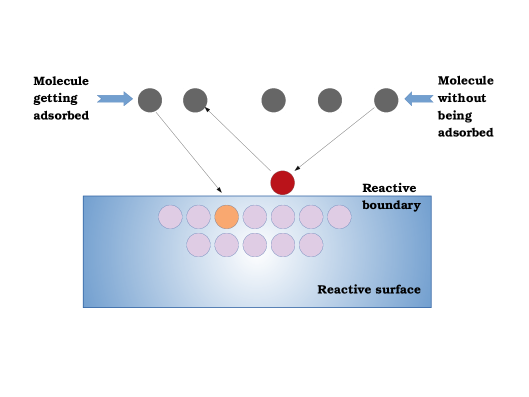
The simplest types of boundary conditions can be formulated in terms of either vanishing flux through the boundary (usually called reflecting or impermeable boundary) or vanishing density at the boundary (called absorbing boundary) Zwanzig90 ; Allison85 ; Lamm83 ; Chapman16 ; Vrentas89 ; Erban07 ; Hattne05 ; Naqvi82 ; Jacob-2012 ; El-Sh-2000 ; Goodrich-54 ; Grebenkov-review ; Isaac . In the first case, a diffusing molecule is reflected whenever it hits the boundary, while in the second type of boundary condition a diffusing molecule is removed from the system whenever it hits the boundary, which can be interpreted as the molecule being absorbed at the boundary. However, more realistic boundary conditions can be realized in terms of a partially absorbing boundary (also termed as Robin, radiative or mixed boundary conditionsCrank75 ), which means that a molecule may be absorbed (or reflected) with some probability Hippel ; Slutsky ; Grebenkov15 ; Dickman01 ; Skorokhod59 ; Burdzy04 ; Singer08 ; Batsilas03 ; Berezhkovskii ; Monine (see Fig. 1). From a bio-chemical point of view, this absorption probability depends on the reactivity of the boundary (e.g. on the rate constant of the adsorbing chemical reaction and on the number of available receptors), and on the details of the model. The reactivity constant can also be measured experimentally from the chemical properties of the boundary (see e.g. GrebenkovRMP07 and references therein).

Figure 1: Schematics of a chemically reactive surface. Some Brownian molecules are being adsorbed by the constituents of a reactive surface. Others react with the constituents at the reactive boundary, forming volatile compounds (indicated in red) before being released to the environment. Reactive constants will characterize the nature of such surfaces. This adsorbing phenomena corresponds to a partially absorbing or reactive surface.

It is worth mentioning that the interaction of a diffusive particle with a reactive boundary is also of practical importance, since they offer plentiful industrial applications in surface or colloid science, and materials research Metzler07 . Few examples worth mentioning are: fluid or mass transport in porous media Stapf06 , electric transport in electrolytic cells Sapoval5 , nuclear magnetic resonance (diffusion of spins in confining porous media), and applications to foam relaxation and surfactantsSonin . Other examples can be found in physiology where oxygen molecules can penetrate across alveolar membranes for further adsorption in blood, or are bounced back and continue the motion. The proportion of adsorbed and reflected oxygen molecules can be characterized by permeability varying from zero (perfectly reflecting boundary) to infinity (perfectly adsorbing boundary) Weibel ; Filoche ; Sapoval1 . A similar description can be useful to explain heterogeneous catalysis frequently observed in petrochemistry e.g. chemical vapor decomposition or plasma etching Vrentas89 . The reactive molecules are injected into a solvent and then they diffuse towards a catalyst. Hitting the catalytic surface, they can be either transformed into other molecules (with a finite reaction rate), or are bounced back for further diffusion in the bulk Sapoval2 ; Sapoval3 ; Sapoval4 .

In this paper we investigate the motion of non-interacting diffusing molecules inside a reactive domain. If left alone the molecules may eventually decay or get adsorbed at the boundary of the confining domain after some time. This is called the lifetime when the molecule gets adsorbed. Clearly, this time is a random quantity whose cumulative probability, called the survival probability, simply measures the chance for the species to remain inside a confining domain up to a fixed time $t$ without being adsorbed or decay. In the literature, computing this distribution is known as the first passage time problem and it has been the subject of interest to scientists for many decades BMS13 ; Majumdar:2005 ; Redner ; First-Passage-Book ; Benichou2011RMP . First passage time problems have ubiquitous applications in physical, biological and chemical processes, ranging from finance to animal foraging theory. Few examples are: survival time of a bacteria to remain alive while searching for food, average lifetime of a messenger RNA which is translated into protein by the joint action of transfer RNA (tRNA) and the ribosome, binding time of a protein to an enzyme, search time of animals for food resources, etc. BMS13 ; Majumdar:2005 ; Redner ; First-Passage-Book ; Benichou2011RMP . Motivated by this backdrop, we investigate the survival properties of diffusive particles inside a reactive domain Grebenkov17 ; Salminen11 . In addition, we are also interested in the extreme displacements made by the diffusing particle and time spent per unit length around a spatial point in the presence of reactive boundaries. This time density is also called the local or reaction time. These quantities are important in characterizing the motion of the molecule. Indeed, the extreme displacement describes the geometrical properties of the trajectories of the molecule, while the reaction time describes the temporal distribution of the trajectories over space and, as such, captures the time spent by a molecule nearby a reactive agent placed at a specific region of the space, upon which the reaction takes place.

We here provide a brief summary of our results which can be divided into three parts. In the first part, we obtain exact analytical results for the propagator, survival probability, and the mean adsorption time. In the second part, we compute the distribution of the maximum displacement of the molecule by the method of counting paths. In the third part of the paper we study the statistical properties of the reaction time using the Feynman-Kac method of Brownian functionals in two cases: (i) when the observation time is fixed, and (ii) when the observation time is random. In all cases, we have verified our results by contrasting them to numerical simulations.

The paper is organized as follows. In Sec. II, we introduce the working model and all the relevant observables which we have studied in subsequent sections. In Sec. III, we provide the details of the derivations and present the results. In particular, general expressions for the propagator, survival probability and the mean adsorption time are given in Sec. III.1. These results are used to compute the full statistics of the maximum displacement in Sec. III.2. In Sec. III.4 we investigate the reaction time profile and present associated exact results. Some of the detailed derivations have been relegated to the appendix Sec. VII for clarity. We conclude our paper in Sec. V.

II Definitions and notations of the quantities of interest

Here we provide the definitions and notations of the quantities that we are interested to study and while doing so we also briefly review the basic concepts and interpretations in the context of a Brownian molecule in presence of reactive boundaries. Imagine that we want to understand the motion of a protein molecule, e.g. an enzyme inside a cell, whose motion can be well described as a diffusion process, in which the boundaries of the cell can be approximated as reactive boundaries. For simplicity we consider the one-dimensional case in which the particle diffuses inside a domain $x\in[0,L]$. Mathematically, this process is described by a propagator $G_{L}(x,x_{0},t)$ which simply represents the probability density for a molecule to be found at $x$ at time $t$ given that it started at $x_{0}$ at an initial time $t_{0}=0$. It can be shown that the propagator satisfies the diffusion equation subject to the reactive boundary conditions at $x=0$ and $x=L$:

$$\frac{\partial}{\partial t}G_{L}(x,x_{0},t) = D\frac{\partial^{2}}{\partial x^{2}}G_{L}(x,x_{0},t)\,,$$ (1)

$$\frac{\partial}{\partial x}G_{L}(0,x_{0},t) = \alpha_{0}G_{L}(0,x_{0},t)\,,$$ (2)

$$\frac{\partial}{\partial x}G_{L}(L,x_{0},t) = \alpha_{L}G_{L}(L,x_{0},t)\,,$$ (3)

where $D$ is the diffusion constant. For clarity, we will consider deterministic initial conditions, that is, $G_{L}(x,x_{0},0)=\delta(x-x_{0})$. The parameter $\alpha_{0}$ (resp. $\alpha_{L}$) controls how often a molecule hitting the boundary at $x=0$ (resp. $x=L$) will be either reflected or absorbed. By tuning these values one can go from a perfectly reflecting boundary to a perfectly absorbing boundary. The problem of finding the propagator have been considered earlier in several contexts mostly in a semi infinite space with one reactive boundary, for example, with step initial condition for the concentration Ben-naim93 , in target search problems Whitehouse-Martin-Satya , or in diffusion controlled recombinations Sano79 . It has been shown that solving the diffusion equation in a bounded domain with reactive boundary conditions is equivalent to solving the diffusion equation in unbounded domain with “sink” terms Ben-naim93 ; Redner .

From the propagator $G_{L}(x,x_{0},t)$, the survival probability that a molecule has not been absorbed or decomposed till the observation time $t$ is simply given by

$$S_{L}(x_{0},t)=\int_{0}^{L}~{}dx~{}G_{L}(x,x_{0},t)~{}.$$ (4)

A simple interpretation of this expression comes from a path counting argument and works as follows. The propagator contains the contributions from all the statistical paths that start at time $t_{0}=0$ at position a $x_{0}$ and end at time $t$ at position a $x$ without being absorbed at either boundary. There are four types of such paths: those which have never reached either boundary at $x=0$ and $x=L$ in time $t$, those which may have hit one of the boundaries but got reflected and those which may have hit both boundaries and, again, got reflected. The survival probability then gets contribution from all such paths which reach any final point $x\in(0,L)$. Analogously to the concept of the first passage time, one can introduce the first absorption time $t_{a}$, being the time at which a molecule is absorbed at either boundary. If we denote its probability density as $f_{L}(x_{0},t)$, it is easy to see that $S_{L}(x_{0},t)=\text{Prob.}(t_{a}>t|x_{0})=\int_{0}^{t}dt^{\prime}f_{L}(x_{0},t^{\prime})$, which implies $f_{L}(x_{0},t)=-\frac{dS_{L}(x_{0},t)}{dt}$.

A related important quantify that we are interested in is the mean absorption time $T_{L}(x_{0})$ (MAT), which can be computed from the density $f_{L}(x_{0},t)$ as

$$T_{L}(x_{0})=\int_{0}^{\infty}~{}dt~{}tf_{L}(x_{0},t).$$ (5)

The MAT is often considered to be a hallmark quantity due to its ubiquity in problems as diverse as the average search time for a bacterium to find its food, or the mean turnover time to complete a reaction, or the running time of a computer programming. We refer to BMS13 ; Majumdar:2005 ; Redner ; First-Passage-Book ; Benichou2011RMP for a comprehensive review on this subject.

Inside a cellular domain, protein molecules will perform short excursions before they either react to substrates or are absorbed at the boundaries. The nature of these paths depend on several factors such as cell concentration, local density of the surrounding molecules, etc. In this biological scenario, very long trajectories may be detrimental for chemical reactions to occur but can be useful when a longer lifetime of a molecule (i.e. with small absorption at the boundaries) is favored. A qualitative geometric characterization of these trajectories can be provided by the statistics of the molecule’s longest excursion, which is, in fact, the maximum displacement of the Brownian particle till a fixed time $t$.

With this in mind, let us then consider a simpler situation where a molecule is moving on the positive axis with a reactive boundary at the origin $x=0$. Let $M$ be the maximum displacement made by the molecule. The cumulative probability that $M$ is less than $L$ is denoted by

$$H(L,t|x_{0})=\text{Prob}[M\leq L,t|x_{0}]$$

$$=\text{Prob.}\left[\{x(t^{\prime})<L;~{}0\leq t^{\prime}\leq t\}~{}|~{}\text{the~{}molecule~{}did~{}not~{}get~{}absorbed~{}at~{}the~{}reactive~{}boundary}~{}x=0\right]$$

$$=\frac{\text{Prob.}[\text{In~{}time~{}{\it t}~{}the~{}molecule~{}did~{}never~{}hit~{}}x=L~{}\text{and~{}did~{}not~{}get~{}absorbed~{}at~{}}~{}x=0]}{\text{Prob.}[\text{In~{}time~{}{\it t}~{}the~{}molecule~{}did~{}not~{}get~{}absorbed~{}at~{}}x=0]}$$ (6)

$$=\frac{\mathcal{S}_{L}(x_{0},t)}{\mathcal{S}_{\infty}(x_{0},t)},$$ (7)

where $\mathcal{S}_{L}(x_{0},t)=\int_{0}^{L}~{}\mathcal{G}_{L}(x,x_{0},t)$ is the survival probability of the molecule in the presence of a full absorbing boundary at $L$ in addition to a reactive boundary at $x=0$, while $\mathcal{G}_{L}(x,x_{0},t)$ is the propagator which describes such a system. Therefore, $\mathcal{G}_{L}(x,x_{0},t)=\underset{\alpha_{L}\to\infty}{\lim}G_{L}(x,x_{0},t)$ and where we have denoted $\mathcal{S}_{\infty}(x_{0},t)=\underset{L\to\infty}{\lim}\mathcal{S}_{L}(x_{0},t)$. The above definition comes from a very simple path counting argument. The cumulative probability $H(L,t|x_{0})$ gets contribution from all the paths which start from $x_{0}$ and reach somewhere within $x\in(0,L)$ (while staying below $x=L$ throughout) along with the condition that they survived the reactive boundary at $x=0$ till time $t$. Hence this probability is exactly the fraction of paths of duration $t$ that starting from $x_{0}$ never hit $x=L$ among those paths which survive till time $t$ from the reactive boundary at $x=0$. In Sec. III.1 we compute the cumulative probability of the maximum distance traveled by the molecule.

Having reached the desired active site, the protein molecule (e.g. enzyme) reacts with substituents or ligands. For example in the kinetics of an enzymatic reaction mechanism, an enzyme binds to a substrate to form a complex, which in turn releases a product, regenerating the original enzyme. This kind of reaction scheme is due to the pioneering work of Michaelis and Menten who further explained how reaction rates depend on the concentration of the enzyme and the substrate Michaelis-Menten . The reaction or binding time of such process is very relevant in biochemistry since prior knowledge could help improve the efficiency of a chemical reaction through catalysis or by facilitating metabolic pathways. A quantitative definition of this time can be formulated as the following

$$L_{t}(y_{0},x_{0})=\int_{0}^{t}~{}dt^{\prime}~{}\delta[x(t^{\prime})-y_{0}|x_{0}]~{},$$ (8)

which measures the amount of time an enzyme spends around the substrate (located at a given coordinate $y_{0}$) over an interval $0\leq t^{\prime}\leq t$. By construction, this is a functional of the trajectory and normalized as $\int dy_{0}~{}L_{t}(y_{0},x_{0})=t$. In the theory of stochastic processes, this is often termed as the local time in diffusion processes Majumdar:2005 ; Sanjib-Satya or the empirical density (when appropriately rescaled by the observation time) in generic Markov processes Donsker-Varadhan ; Barato . In section Sec. III.4 we will use the Feynman-Kac path integral formalism to investigate the statistical properties of this Brownian functional.

III Main Results

III.1 Propagator, survival probability and the mean absorption time

This section contains our main results on the quantities discussed in the previous section and their explicit derivations. To compute these quantities we first need to solve Eq. (1) to find the propagator inside the domain $x\in[0,L]$ satisfying the reactive boundary conditions Eq. (2) and Eq. (3) and the initial condition

$$G_{L}(x,x_{0},t=0)=\delta(x-x_{0}).$$ (9)

Applying the method of separation of variables in Eq. (1) we can write the propagator in the following way

$$G_{L}(x,x_{0},t)=\underset{k}{\sum}~{}c_{k}~{}\psi_{k}(x)~{}\psi_{k}(x_{0})~{}e^{-Dk^{2}~{}t},$$ (10)

where the $k$’s are the eigenvalues whose corresponding eigenfunctions $\psi_{k}(x)$ satisfy

$$\frac{\partial^{2}\psi_{k}(x)}{\partial x^{2}}=-k^{2}\psi_{k}(x),$$ (11)

with the boundary conditions (BCs)

$$\frac{\partial}{\partial x}\psi_{k}(x,t)\Big{|}_{x\to 0} = \alpha_{0}\psi_{k}(x,t)\Big{|}_{x\to 0}\,,$$ (12)

$$\frac{\partial}{\partial x}\psi_{k}(x,t)\Big{|}_{x\to L} = \alpha_{L}\psi_{k}(x,t)\Big{|}_{x\to L}\,.$$ (13)

A general solution of Eq. (11) is given by

$$\psi_{k}(x)=a(k)\cos(kx)+b(k)\sin(kx).$$ (14)

To determine the functions $a(k)$ and $b(k)$ we insert $\psi_{k}(x)$ back into Eqs. (12) and (13) to obtain

$$kb(k) = \alpha_{0}a(k),$$ (15)

$$\tan(kL) = \frac{kb(k)-\alpha_{L}a(k)}{ka(k)+\alpha_{L}b(k)}\,.$$ (16)

Now, assuming that $a(k)=kf(k)$ and $b(k)=\alpha_{0}f(k)$ for some $f(k)$ to be determined from normalization, we have from Eq. (16) that

$$e^{2ikL}=\frac{(k+i\alpha_{0})(k-i\alpha_{L})}{(k-i\alpha_{0})(k+i\alpha_{L})},$$ (17)

and from Eq. (11)

$$\psi_{k}(x)=f(k)~{}[k\cos(kx)+\alpha_{0}\sin(kx)].$$ (18)

Hence, the full solution reads

$$G_{L}(x,x_{0},t)=\underset{k\in\mathcal{R}_{k}(L)}{\sum}~{}C_{k}~{}[k\cos(kx)+\alpha_{0}\sin(kx)]~{}[k\cos(kx_{0})+\alpha_{0}\sin(kx_{0})]~{}e^{-Dk^{2}~{}t},$$ (19)

where $C_{k}=c_{k}f^{2}(k)$ is a constant to be determined, and $\mathcal{R}_{k}(L)$ is the set of eigenvalues, solution of the transcendental equation (17), for a fixed value of $L$. In the context of finding the reunion probability of $N$ Brownian particles moving on a line with partially absorbing/reflecting crossing conditions, a general multi-particle propagator has been computed using Bethe ansatzIsaac . The constant $C_{k}$ in Eq. (19) can now be found using the initial condition in Eq. (9)

$$C_{k}\psi_{k}(x_{0}) = \frac{\int_{0}^{L}~{}dx~{}G_{L}(x,x_{0},0)\psi_{k}(x)}{\int_{0}^{L}~{}dx~{}\psi_{k}(x)\psi_{k}(x)}\,,$$ (20)

where we have assumed that the set of normalized eigenfunctions $\psi_{k}(x)$ forms a complete basis in $[0,L]$ with $k\in\mathcal{R}_{k}(L)$. Performing a lengthy manipulation we obtain the normalization to be

$$C_{k}=(\alpha_{0}^{2}+k^{2})^{-1}\left[L+\frac{\alpha_{0}}{\alpha_{0}^{2}+k^{2}}-\frac{\alpha_{L}}{\alpha_{L}^{2}+k^{2}}\right]^{-1}~{}.$$ (21)

Substituting this result in Eq. (19), we arrive at the final expression for the full propagator

$$G_{L}(x,x_{0},t) = \underset{k\in\mathcal{R}_{k}(L)}{\sum}~{}e^{-Dk^{2}t}~{}\frac{[k\cos(kx)+\alpha_{0}\sin(kx)]~{}[k\cos(kx_{0})+\alpha_{0}\sin(kx_{0})]}{(\alpha_{0}^{2}+k^{2})\left[L+\frac{\alpha_{0}}{\alpha_{0}^{2}+k^{2}}-\frac{\alpha_{L}}{\alpha_{L}^{2}+k^{2}}\right]}\,.$$ (22)

Various limits can be immediately examined from Eq. (22). For example, in the case of a semi-infinite domain (where the boundary at $x=L$ is taken to infinity) the propagator takes the following form (see Sec. VII.1 for details)

$$G^{\text{si}}(x,x_{0},t)=\frac{1}{4\alpha_{0}}~{}e^{D\alpha_{0}^{2}t}~{}\mathcal{D}_{x}\mathcal{D}_{x_{0}}~{}\Big{[}\phi(x-x_{0},t)-\phi(x+x_{0},t)\Big{]}~{},$$ (23)

where $\mathcal{D}_{y}=\Big{(}\frac{\partial}{\partial y}+\alpha_{0}\Big{)}$, and the function $\phi$ is defined as follows

$$\phi(z,t)=e^{\alpha_{0}z}\mathrm{erfc}\Big{[}\frac{2D\alpha_{0}t+z}{\sqrt{4Dt}}\Big{]}~{}+~{}e^{-\alpha_{0}z}\mathrm{erfc}\Big{[}\frac{2D\alpha_{0}t-z}{\sqrt{4Dt}}\Big{]}.$$ (24)

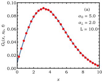
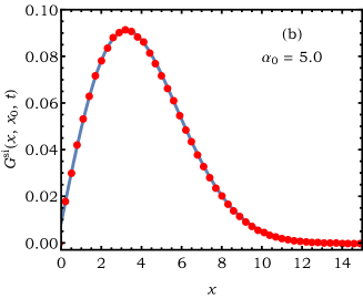
In Fig. 2, we have compared our analytical results to Monte Carlo simulations, which were performed according to the method explained in Sec. IV. The left panel, corresponds to taking a finite size interval, while the right panel is the result of considering a semi-infinite domain. In both cases the agreement between theory and Monte Carlo simulations is excellent.

Figure 2: We have simulated the motion of a Brownian molecule inside the interval $[0,L]$ with reactive boundaries at $x=0$ and $x=L$. We have measured the displacement of the molecule till an observation time $t=5$ for two individual cases. In the left panel (a), we show the probability distribution of the molecule displacement when it diffuses strictly inside the box. We plot this numerical measurement (in red circles) with Eq. (22) (in solid line) and find an excellent match. In the right panel (b), we have considered the semi-infinite domain by taking the boundary at $L$ to be at infinity and measured the probability distribution of its displacement. The simulation data (in red circle) is plotted against the theoretical formula (in solid line) obtained using Eq. (23).

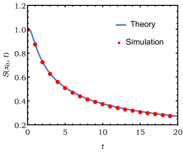
Figure 3: Comparison of the expression Eq. (26) of the survival on the semi-infinite line with a reactive boundary at the origin with an estimate obtained from numerical simulations. We have used the following parameters for the simulation: $\alpha_{0}=5.0$ and $x_{0}=2.0$. The simulation data (in red circles) is in excellent agreement with the analytical result (in solid line).

Once we have obtained an exact expression for the propagator $G_{L}(x,x_{0},t)$ we can move on to derive the expressions for the survival probability and the mean absorption time.

Survival probability: The survival probability $S_{L}(x_{0},t)$ inside the interval $[0,L]$ with reactive boundaries is a quantitative measure of the probability that the Brownian molecule survives without being absorbed by neither boundary. This probability is obtained by integrating the final position $x$ from $0$ to $L$ in the expression of the propagator $G_{L}(x,x_{0},t)$, yielding:

$$S_{L}(x_{0},t)=\underset{k\in\mathcal{R}_{k}}{\sum}~{}e^{-Dk^{2}t}~{}\frac{\Big{[}\alpha_{0}(1-\cos(kL))+k\sin(kL)\Big{]}~{}[k\cos(kx_{0})+\alpha_{0}\sin(kx_{0})]}{k(\alpha_{0}^{2}+k^{2})\left[L+\frac{\alpha_{0}}{\alpha_{0}^{2}+k^{2}}-\frac{\alpha_{L}}{\alpha_{L}^{2}+k^{2}}\right]}\,.$$ (25)

In the limit of $L\to\infty$ (semi-infinite domain), the survival probability at the boundary $0$ till an observation time $t$ can either be obtained from Eq. (25) , or by integrating out the final position $x$ in $G^{\text{si}}(x,x_{0},t)$ from zero to infinity. Either way, the final result is

$$S(x_{0},t)=e^{D\alpha_{0}^{2}t+\alpha_{0}x_{0}}~{}\mathrm{erfc}\Big{[}\frac{x_{0}+2D\alpha_{0}t}{\sqrt{4Dt}}\Big{]}+\mathrm{erf}\Big{[}\frac{x_{0}}{\sqrt{4Dt}}\Big{]}\,,$$ (26)

which, as shown in Fig. 3, agrees with estimates obtained by Monte Carlo simulations. It is easy to verify from Eq. (26) that when the boundary is completely reflective (i.e. $\alpha_{0}\to 0$) the process always survives, that is $S(x_{0},t)=1$. On the other hand, for a completely absorbing boundary condition (i.e. $\alpha_{0}\to\infty$) we readily recover the canonical result $S(x_{0},t)=\mathrm{erf}\Big{[}x_{0}/\sqrt{4Dt}\Big{]}$ Redner . Next, we focus on the mean absorption time.

Mean absorption time (MAT): The explicit form of the survival probability allows us to compute the first absorption time density immediately. The distribution $f_{L}(t,x_{0})$ of the absorption time is given by $f_{L}(t,x_{0})=-dS_{L}(x_{0},t)/dt$, from which the MAT reads

$$T_{L}(x_{0})=\underset{k\in\mathcal{R}_{k}}{\sum}~{}\frac{\Big{[}\alpha_{0}(1-\cos(kL))+k\sin(kL)\Big{]}~{}[k\cos(kx_{0})+\alpha_{0}\sin(kx_{0})]}{Dk^{3}(\alpha_{0}^{2}+k^{2})\left[L+\frac{\alpha_{0}}{\alpha_{0}^{2}+k^{2}}-\frac{\alpha_{L}}{\alpha_{L}^{2}+k^{2}}\right]}.$$ (27)

In the presence of two completely absorbing boundaries at $0$ and at $L$ (that is, by taking the limits $\alpha_{0}\to\infty$ and $\alpha_{L}\to\infty$), the MAT takes the following form

$$T_{L}^{\text{abs}}(x_{0})=\frac{2L^{2}}{D\pi^{3}}\sum\limits_{n=1}^{\infty}\frac{1-(-1)^{n}}{n^{3}}\sin\left(\frac{n\pi x_{0}}{L}\right)=\frac{L^{2}}{2D}~{}z(1-z)~{},$$ (28)

where $z=x_{0}/L$ and thus we recover this previously obtained resultRedner ; Satya-Krapivsky2010 . On the other hand, by taking the semi-infinite limit ($L\to\infty$) with finite $\alpha_{0}$ , the MAT diverges, as expected Redner .

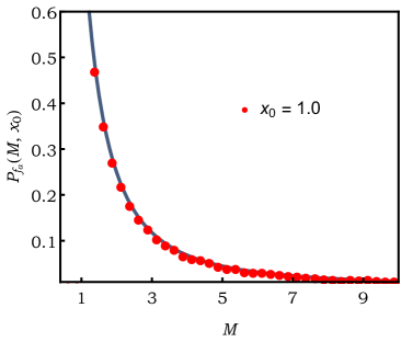
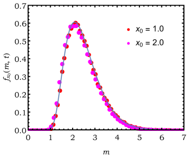
Figure 4: Left panel: we have plotted the scaled probability distribution $f_{x_{0}}(m,t)$ as a function of the scaled maximum displacement $m$. The point symbols represent data obtained from the Monte-Carlo simulations. The red and the magenta symbols indicate data sets for $x_{0}=1.0$ and $x_{0}=2.0$, respectively. The solid line represents the theoretical curve from Eq. (33). An excellent data collapse for the scaled distribution is observed for different initial conditions, as predicted from our analysis. Right panel: we show the probability distribution of the maximum excursion $P_{f_{a}}(M,x_{0})$ performed by the molecule before it is absorbed by the reactive boundary at the origin. The red circles are obtained from simulations and plotted against the solid curve obtained from the theoretical result using Eq. (37). The parameters for this figure are: $D=1,~{}\alpha_{0}=5.0$, observation time $t=100.0$, and $x_{0}=1.0$.

III.2 Distribution of maximum displacement till a fixed time $t$

In this section, we study the statistics of the maximum displacement of our diffusing molecule. Often the amount of space visited by a diffusing chemical reagent inside a cell becomes quite important as it might control the yield of a reaction. One of the simplest measures of such excursions in one dimension is the maximum displacement traversed by the molecule.

In order to calculate the statistics of the maximum, it is convenient to introduce the probability that the maximum displacement $M$ is less than or equal to $L$ (in 1D). To compute this cumulative distribution, one imposes an adsorbing boundary at $x=L$ which is equivalent to taking $\alpha_{L}\to\infty$ in the original problem with two reactive boundaries. Taking this limit in Eq. (22), we get the corresponding propagator

$$\mathcal{G}_{L}(x,x_{0},t)=\lim\limits_{\alpha_{L}\to\infty}G_{L}(x,x_{0},t) = \sum\limits_{k}\dfrac{[k\cos(kx)+\alpha_{0}\sin(kx)]~{}[k\cos(kx_{0})+\alpha_{0}\sin(kx_{0})]}{L(\alpha_{0}^{2}+k^{2})+\alpha_{0}}~{}e^{-Dk^{2}t},$$

with $$~{}~{}~{}~{}e^{2ikL}=\frac{(k+i\alpha_{0})}{(k-i\alpha_{0})},$$ (29)

which was defined in Sec. II. Integrating the final position $x$ of this propagator from $0$ to $L$, we get the associated survival probability $\mathcal{S}_{L}(x_{0},t)$ of the particle:

$$\mathcal{S}_{L}(x_{0},t)=\int_{0}^{L}dx~{}\mathcal{G}_{L}(x,x_{0},t).$$ (30)

Once we know $\mathcal{S}_{L}(x_{0},t)$, the cumulative distribution of the maximum $M$ is obtained from the ratio (see Eq. (7))

$$H(L,t|x_{0})=\text{Prob.}[M\leq L,t|x_{0}]=\frac{\mathcal{S}_{L}(x_{0},t)}{\mathcal{S}_{\infty}(x_{0},t)}~{}~{}~{}\text{where}~{}~{}~{}\mathcal{S}_{\infty}(x_{0},t)=\lim\limits_{L\to\infty}\mathcal{S}_{L}(x_{0},t).$$ (31)

Clearly, in the limits $L\to\infty$ and $t\to\infty$, while keeping $\ell=\frac{L}{\sqrt{Dt}}$ constant, the survival probability $\mathcal{S}_{L}(x_{0},t)$ can be written in terms of the scaled variable $z_{0}=\frac{x_{0}}{\sqrt{Dt}}$ such that $\mathcal{S}_{L}(x_{0},t)=s_{\ell}(z_{0},t)$. After performing some algebraic manipulations one derives

$$s_{\ell}(z_{0},t)\simeq 2\alpha_{0}\sqrt{Dt}~{}\ell^{2}~{}\sum\limits_{n=1}^{\infty}\frac{[1-(-1)^{n}]\left[\frac{n\pi}{\ell}\cos\left(\frac{n\pi z_{0}}{\ell}\right)+\sqrt{Dt}\alpha_{0}\sin\left(\frac{n\pi z_{0}}{\ell}\right)\right]}{n\pi\left[n^{2}\pi^{2}+Dt~{}\alpha_{0}^{2}~{}\ell^{2}+\sqrt{Dt}~{}\alpha_{0}~{}\ell\right]}~{}e^{-\frac{n^{2}\pi^{2}}{\ell^{2}}}.$$ (32)

To arrive at the above expression we have replaced $kL=p\ell$ in Eq. (29) to obtain the transcendental equation $\frac{p}{\tan(p\ell)}=-\alpha_{0}\sqrt{Dt}$. For large $t$, the solution of this equation is given approximately by $p\approx\frac{n\pi}{\ell}$ with $n=1,2,3...$. Hence by taking a derivative in Eq. (31), we obtain the following scaling form for the distribution $P_{x_{0}}(M,t)$ of the maximum

$$P_{x_{0}}(M,t)=\frac{1}{\sqrt{Dt}}~{}f_{x_{0}/\sqrt{Dt}}\left(\frac{M}{\sqrt{Dt}},t\right),~{}~{}~{}\text{where}~{}~{}f_{z_{0}}(m,t)=\frac{1}{\lim\limits_{\ell\to\infty}s_{\ell}(z_{0},t)}\left(\frac{\partial s_{\ell}(z_{0},t)}{\partial\ell}\right)_{\ell=m}~{},$$ (33)

is the scaling function with the scaled maximum displacement $m=M/\sqrt{Dt}$. In the left panel of Fig. 4, we have compared the expression of $\sqrt{Dt}P_{x_{0}}(M,t)$, given by Eq. (33), with the corresponding estimate obtained by Monte Carlo simulations. As it can be appreciated in Eq. (33), when plotted in this way we should observe a data collapse for various values of the initial position $x_{0}$ and, indeed, this is what we have obtained numerically.

For an absorbing boundary at $x=0$ ( $\alpha_{0}\to\infty$), the root equation in Eq. (29) becomes $\tan(p\ell)=0$. This gives us the solutions $p\approx\frac{n\pi}{\ell}$ for $n=1,2,3...$, from which we derive the following form of the scaled survival probability

$$s_{\ell}(z_{0},t)=\frac{2}{\pi}\sum\limits_{n=1}^{\infty}\frac{1-(-1)^{n}}{n}~{}\sin\left(\frac{n\pi z_{0}}{\ell}\right)~{}e^{-\frac{n^{2}\pi^{2}}{\ell^{2}}}~{},$$ (34)

which matches with the result derived previously in Satya-Krapivsky2010 .

III.3 Distribution of maximum displacement till the first absorption time

It is also fairly important to know up to what extent the molecule has explored a region before it got absorbed at the reactive boundary. This can be quantified by the maximum displacement $M$ made by the molecule till the absorption time. The cumulative distribution $Q_{a}(L|x_{0})=\text{Prob.}[M\leq L|x_{0}]$ of this maximum $M$ can be obtained from

$$Q_{a}(L|x_{0})=D\int_{0}^{\infty}dt~{}\left(\frac{\partial\mathcal{G}_{L}}{\partial x}\right)_{x=0}.$$ (35)

After using the expression of $\mathcal{G}_{L}$ from Eq. (29) and performing some manipulations we get

$$Q_{a}(L|x_{0})=\alpha_{0}\sum_{k}\frac{[k\cos(kx_{0})+\alpha_{0}\sin(kx_{0})]}{k[\alpha_{0}+L(\alpha_{0}^{2}+k^{2})]},~{}~{}~{}~{}~{}\text{with}~{}~{}~{}e^{2ikL}=\frac{(k+i\alpha_{0})}{(k-i\alpha_{0})}.$$ (36)

Hence, the distribution of the maximum $P_{a}(M,x_{0})$ till absorption time is obtained from

$$P_{f_{a}}(M,x_{0})=\left(\frac{\partial Q_{a}(L|x_{0})}{\partial L}\right)_{L=M}.$$ (37)

We have plotted Eq. (37) against numerical simulations in Fig. 4 (right panel) and we observe an excellent agreement between them. In this case, one can also check the various limits which have been studied earlier. For example, in case of a fully absorbing boundary at $x=0$ ($\alpha_{0}\to\infty$), one can show that the scaled cumulative distribution is given by

$$Q_{a}(z_{0},\ell)=2\sum\limits_{n=1}^{\infty}\frac{\sin\left(\frac{n\pi x_{0}}{L}\right)}{n\pi}=1-\frac{x_{0}}{L}\,,$$ (38)

which reproduces the result derived in Satya-Krapivsky2010 .

III.4 Reaction time spent at $y_{0}$ till observation time $t$:

Let us now focus our attention at studying the time spent by the molecule at some particular point while being observed for a time interval $t$. In the introduction we have mentioned examples where the characterization of the reaction time renders subtle information about chemical or metabolic reactions. Here we show how one can shed some light into the statistical properties of the reaction time for this paradigmatic model. For convenience, let us recall the definition of the reaction time spent by a Brownian molecule at reaction coordinate $y_{0}$ given that it started at $x_{0}$, or, in other words,

$$L_{t}(y_{0},x_{0})=\int_{0}^{t}~{}dt^{\prime}~{}\delta[x(t^{\prime})-y_{0}|x_{0}]~{},$$ (39)

where the observation time $t$ is fixed. Sometimes, this time can be taken stochastic, as we discussed in Sec. III.5.

In order to compute the statistical properties of $L_{t}$, we introduce the generating function

$$\mathcal{Q}_{p}(y_{0},x_{0},t)=\langle e^{-pL_{t}(y_{0},x_{0})}\rangle$$ (40)

where the average is performed with respect to the probability density $P(L_{t}|x_{0},y_{0},t)$ of the reaction time. This average can be written explicitly after taking into account the exact path measure

$$\mathcal{Q}_{p}(y_{0},x_{0},t)=\frac{1}{S_{L}(x_{0},t)}~{}\int_{0}^{L}~{}dx~{}\int_{x(0)=x_{0}}^{x(t)=x}~{}\mathcal{D}[x(\tau)]~{}e^{-\int_{0}^{t}~{}d\tau\left[\frac{1}{4D}\left(\frac{dx(\tau)}{d\tau}\right)^{2}+p\delta(x(\tau)-y_{0})\right]}\,,$$ (41)

where the survival probability $S_{L}(x_{0},t)$ weighs the surviving paths (see Eq. (25)). Following the Feynman-Kac method and after introducing an appropriate Hamiltonian $H_{p}$, one can map the original problem of evaluating the above path integral into the computation of an imaginary time quantum propagator:

$$\mathcal{Q}_{p}(y_{0},x_{0},t) =\frac{Q_{p}(y_{0},x_{0},t)}{S_{L}(x_{0},t)}\,,$$ (42)

where

$$Q_{p}(y_{0},x_{0},t) =\int_{0}^{L}~{}dx~{}\langle x|e^{-t\hat{H}_{p}}|x_{0}\rangle\,,$$ (43)

$\hat{H}_{p}(y_{0})=-D\frac{d^{2}}{dx^{2}}+p~{}\delta(x-y_{0})$, and $S_{L}(x_{0},t)=\int_{0}^{L}~{}dx~{}\langle x|e^{-t\hat{H}_{0}}|x_{0}\rangle$. Using the backward Kolmogorov approach one can show that $Q_{p}(y_{0},x_{0},t)$ obeys the following Fokker-Planck equation:

$$\frac{\partial Q_{p}}{\partial t}=D\frac{\partial^{2}Q_{p}}{\partial x_{0}^{2}}-p\delta(x_{0}-y_{0})Q_{p}\,,$$ (44)

with $Q_{p}(y_{0},x_{0},0)=1$, and boundary conditions

$$~{}~{}\left[\frac{\partial Q_{p}}{\partial x_{0}}-\alpha_{0}Q_{p}\right]_{x_{0}=0}=0\,,\quad\quad\left[\frac{\partial Q_{p}}{\partial x_{0}}-\alpha_{L}Q_{p}\right]_{x_{0}=L}=0\,.$$ (45)

The usual trick is then to write Eq. (44) in Laplace space with $\tilde{Q}_{p}(y_{0},x_{0},s)=\int_{0}^{\infty}dt~{}e^{-st}Q_{p}(y_{0},x_{0},t)$ such that

$$D\frac{d^{2}\tilde{Q}_{p}}{dx_{0}^{2}}-[s+p~{}\delta(x_{0}-y_{0})]\tilde{Q}_{p}=-1\,.$$ (46)

The boundary conditions in Eq. (45) are automatically translated into

$$\left[\frac{\partial\tilde{Q}_{p}}{\partial x_{0}}-\alpha_{0}\tilde{Q}_{p}\right]_{x_{0}=0}=0,\quad\quad\left[\frac{\partial\tilde{Q}_{p}}{\partial x_{0}}-\alpha_{L}\tilde{Q}_{p}\right]_{x_{0}=L}=0\,.$$ (47)

Although a formal solution of Eq. (44) does exist, the exact Laplace inversion of $\tilde{Q}_{p}(y_{0},x_{0},s)$ turns out to be rather difficult. However, we notice that a few exact results are available for the generating function $\mathcal{Q}_{p}(y_{0},x_{0},t)$ and for $P(L_{t}|x_{0},y_{0},t)$ when one approaches the limit of the semi-infinite domain. In the rest of this section we thus focus on this particular limit. The interpretation of the generating function $\mathcal{Q}_{p}(y_{0},x_{0},t)$ is now extended accordingly to

$$\mathcal{Q}_{p}(y_{0},x_{0},t) = \frac{Q_{p}(y_{0},x_{0},t)}{S(x_{0},t)}\,,$$ (48)

$$Q_{p}(y_{0},x_{0},t) = \int_{0}^{\infty}~{}dx~{}\langle x|e^{-t\hat{H}_{p}}|x_{0}\rangle\,,$$ (49)

where $S(x_{0},t)$ is given by Eq. (26), while the governing equation for $\tilde{Q}_{p}(y_{0},x_{0},s)$ is still given by Eq. (44) with new boundary conditions

$$\left[\frac{\partial\tilde{Q}_{p}}{\partial x_{0}}-\alpha_{0}\tilde{Q}_{p}\right]_{x_{0}=0}=0 \quad\quad\tilde{Q}_{p}(y_{0},x_{0},s)|_{x_{0}\to\infty}=\frac{1}{s}~{}.$$ , (50)

The second boundary condition is obtained from the fact that as $x_{0}\to\infty$, the local time $L_{t}\to 0$ which results into $Q_{p}\to 1$. To obtain the complete solution of $\tilde{Q}_{p}(y_{0},x_{0},s)$, we need to solve Eq. (44) with the new boundary conditions given by Eq. (50) in two different regions separately. These are: (I) $0\leq x_{0}\leq y_{0}$, and (II) $x_{0}\geq y_{0}$. A general solution in these two regions can be written as

$$\tilde{Q}_{p}^{(I)}(y_{0},x_{0},s) = A~{}e^{-x_{0}\sqrt{s/D}}+B~{}e^{-x_{0}\sqrt{s/D}}+\frac{1}{s},~{}~{}~{}\text{for}~{}~{}0\leq x_{0}\leq y_{0}$$ (51)

$$\tilde{Q}_{p}^{(II)}(y_{0},x_{0},s) = C~{}e^{-x_{0}\sqrt{s/D}}+\frac{1}{s},~{}~{}~{}~{}~{}~{}~{}~{}~{}~{}~{}~{}~{}~{}~{}~{}~{}~{}~{}~{}~{}~{}~{}~{}~{}\text{for}~{}~{}x_{0}\geq y_{0}.$$ (52)

The constants $A$, $B$ and $C$ can be obtained from the following conditions

• Condition (a) : Boundary condition at $x_{0}=0$, i.e., $\frac{\partial\tilde{Q}_{p}}{\partial x_{0}}-\alpha_{0}\tilde{Q}_{p}\big{|}_{x_{0}=0}=0$, which implies

  $$B(\sqrt{s/D}-\alpha_{0})-A(\sqrt{s/D}+\alpha_{0})=\frac{\alpha_{0}}{s}.$$ (53)

• Condition (b) : Continuity of the solution at $x_{0}=y_{0}$, which implies

  $$Be^{y_{0}\sqrt{s/D}}+Ae^{-y_{0}\sqrt{s/D}}=Ce^{-y_{0}\sqrt{s/D}}.$$ (54)

  Solving Eqs. (53) and (54) for $A$ and $B$, we get the following expressions in terms of $C$

  $$Ae^{-y_{0}\sqrt{s/D}} = \frac{\sqrt{D}}{2R_{y_{0}}(s)}\left(-\frac{\alpha}{s}+C~{}(\sqrt{s/D}-\alpha_{0})~{}e^{-2y_{0}\sqrt{s/D}}\right),$$ (55)

  $$Be^{y_{0}\sqrt{s/D}} = \frac{\sqrt{D}}{2R_{y_{0}}(s)}\left(\frac{\alpha}{s}+C~{}(\sqrt{s/D}+\alpha_{0})\right),~{}~{}~{}\text{where},$$ (56)

  $$R_{y_{0}}(s) = \sqrt{s}\cosh(y_{0}\sqrt{s/D})+\alpha_{0}\sqrt{D}\sinh(y_{0}\sqrt{s/D}).$$ (57)

• Condition (c) : Discontinuity of the first derivative at $x_{0}=y_{0}$, i.e.,

  $$\frac{\partial\tilde{Q}_{p}^{(II)}}{\partial x_{0}}\big{|}_{x_{0}=y_{0}}-\frac{\partial\tilde{Q}_{p}^{(I)}}{\partial x_{0}}\big{|}_{x_{0}=y_{0}}=\frac{p}{D}\tilde{Q}_{p}^{(II)}(y_{0},y_{0},s).$$ (58)

  Using the expressions of $A$ and $B$ from Eqs. (55) and (56) in the above equation we get

  $$C~{}e^{-y_{0}\sqrt{s/D}}=-\frac{1}{s}~{}\frac{pR_{y_{0}}(s)+\alpha_{0}D\sqrt{s}}{pR_{y_{0}}(s)+\sqrt{s}(\sqrt{sD}+\alpha_{0}D)~{}e^{y_{0}\sqrt{s/D}}}.$$ (59)

Using this expression of $C$ in Eqs. (55) and (56) we get explicit expressions of $A$ and $B$. As a result we have a complete specification of $\tilde{Q}_{p}(y_{0},x_{0},s)$, from which performing double inverse Laplace transformation one can, in principle, obtain $P(L_{t}|x_{0},y_{0},t)$ for any reaction location $y_{0}$. In the following we consider two choices for this location to demonstrate few exact results. The choices are: (i) at the origin ($y_{0}=0$), and (ii) at its initial position $y_{0}=x_{0}$.

III.4.1 Reaction time around the reactive boundary $y_{0}=0$

In this case, $R_{y_{0}}(s)=\sqrt{s}$. Hence, the constant $C$ in Eq. (59) now reads

$$C=-\frac{1}{s}~{}\frac{p+\alpha_{0}D}{p+\alpha_{0}D+\sqrt{sD}},$$ (60)

and as a result the function $\tilde{Q}_{p}(0,x_{0},s)$ has the following form

$$\tilde{Q}_{p}(0,x_{0},s) = \frac{1}{s}-\frac{1}{s}~{}\frac{p+\alpha_{0}D}{p+\alpha_{0}D+\sqrt{sD}}~{}e^{-x_{0}\sqrt{s/D}},$$ (61)

$$= \frac{1-e^{-x_{0}\sqrt{s/D}}}{s}+\frac{e^{-x_{0}\sqrt{s/D}}}{\sqrt{s}(p+\alpha_{0}D+\sqrt{sD})}\,.$$

Performing the inverse Laplace transform with respect to $s$ we obtain

$$Q_{p}(0,x_{0},t) = S(x_{0},t)~{}\mathcal{Q}_{p}(0,x_{0},t)=e^{D\alpha_{p}^{2}t+\alpha_{p}x_{0}}\text{erfc}\left(\frac{2D\alpha_{p}t+x_{0}}{\sqrt{4Dt}}\right)+\text{erf}\left(\frac{x_{0}}{\sqrt{4Dt}}\right),$$ (62)

where $\alpha_{p}=\alpha_{0}+\frac{p}{D}$. Now performing the inverse Laplace transform with respect to $p$, we get

$$q_{0}(L_{t},t|x_{0})=\mathcal{L}^{-1}_{L_{t}}(Q_{p}(0,x_{0},t))=2~{}\text{erf}\left(\frac{x_{0}}{\sqrt{4Dt}}\right)~{}\delta(L_{t})+\sqrt{\frac{D}{\pi t}}~{}e^{-\alpha_{0}L_{t}D}~{}e^{-\frac{(x_{0}+L_{t}D)^{2}}{4Dt}}~{}.$$ (63)

Hence, the distribution of the local time (density) at $y_{0}=0$ is given by

$$P(L_{t}|x_{0},0,t) = \frac{1}{S(x_{0},t)}~{}\left[2~{}\text{erf}\left(\frac{x_{0}}{\sqrt{4Dt}}\right)~{}\delta(L_{t})+\sqrt{\frac{D}{\pi t}}~{}e^{-\alpha_{0}L_{t}D}~{}e^{-\frac{(x_{0}+L_{t}D)^{2}}{4Dt}}\right],$$

where $$S(x_{0},t)=e^{D\alpha_{0}^{2}t+\alpha_{0}x_{0}}\text{erfc}\left(\frac{2D\alpha_{0}t+x_{0}}{\sqrt{4Dt}}\right)+\text{erf}\left(\frac{x_{0}}{\sqrt{4Dt}}\right).$$ (64)

The $\delta(L_{t})$ term in Eq. (63) arises from those paths which are absorbed at the reactive boundary upon their first passage. The factor $\text{erf}({x_{0}}/{\sqrt{4Dt}})/S(x_{0},t)$ represents the fraction of those paths, which starting at $x_{0}$ survived being absorbed by the reactive boundary and, moreover, did not make any visit to the boundary till time $t$. Note that this is the term that survives in the $\alpha_{0}\to\infty$ limit, i.e., when the boundary becomes completely absorbing.

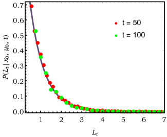
Figure 5: Numerical distribution of reaction time $L_{t}$ till the observation time $t$, starting from $x_{0}$. We measure the reaction time around its initial coordinate i.e., $y_{0}=x_{0}$ here. The point symbols (red and green) represent simulation data obtained for time $(t=50$ and $100)$ respectively. The solid line is obtained from the theoretical result in Eq. (70). Since Eq. (70) does not depend on $t$, we see all the data fall in the same line. The parameters for this figure are: $D=1,y_{0}=x_{0}=0.5$, and $\alpha_{0}=5.0$.

III.4.2 Reaction time around its initial position $y_{0}=x_{0}$

Putting $y_{0}=x_{0}$ in Eqs. (51) and (52), and using the expression of $C$ from Eq. (59) we have

$$\tilde{Q}_{p}(x_{0},x_{0},s)=\frac{1}{s}+C~{}e^{-x_{0}\sqrt{s/D}}=\frac{1}{s}~{}\frac{s\sqrt{D}+\alpha_{0}D\sqrt{s}(1-e^{-y_{0}\sqrt{s/D}})}{R_{y_{0}}(s)e^{-x_{0}\sqrt{s/D}}}~{}\times~{}\frac{1}{p+\frac{s\sqrt{D}+\alpha_{0}D\sqrt{s}}{R_{x_{0}}(s)}e^{-x_{0}\sqrt{s/D}}},$$ (65)

where $R_{x_{0}}(s)$ is given by Eq. (57). Performing the inverse Laplace transform with respect to $p$ we get

$$\tilde{Z}_{s}(L_{t},x_{0})=\mathcal{L}^{-1}_{L_{t}}(\tilde{Q}_{p}(x_{0},x_{0},s))=\frac{1}{s}~{}\frac{s\sqrt{D}+\alpha_{0}D\sqrt{s}(1-e^{-x_{0}\sqrt{s/D}})}{R_{x_{0}}(s)e^{-x_{0}\sqrt{s/D}}}~{}\times~{}e^{-\frac{s\sqrt{D}+\alpha_{0}D\sqrt{s}}{R_{x_{0}}(s)}e^{-x_{0}\sqrt{s/D}}~{}L_{t}}.$$ (66)

We need to perform another inverse Laplace transform with respect to $s$ to get $Z_{t}(L_{t},x_{0})=\mathcal{L}^{-1}_{s}(\tilde{Z}_{s}(L_{t},x_{0}))$. We can then use this result to obtain the reaction time density $P(L_{t}|x_{0},x_{0},t)$ as

$$P(L_{t}|x_{0},x_{0},t)=\frac{Z_{t}(L_{t},x_{0})}{S(x_{0},t)},$$ (67)

where $S(x_{0},t)$ is the survival probability given by Eq. (64). It seems to be rather cumbersome to perform the second Laplace inversion analytically. However, it is possible to look at the following limits :

• Large $t$ : In this case, the dominant contribution to the inverse Laplace transform with respect to $s$ comes from the small $s$ limit of $\tilde{Z}_{s}(L_{t},x_{0})$ and that is given by

  $$\tilde{Z}_{s}(L_{t},x_{0})|_{s\to 0}\simeq\sqrt{D}~{}e^{-\frac{\alpha_{0}DL_{t}}{1+x_{0}\alpha_{0}}}~{}\frac{1}{\sqrt{s}}~{}e^{-\frac{DL_{t}\sqrt{s}}{1+x_{0}\alpha_{0}}},$$ (68)

  which provides

  $$Z_{t}(L_{t},x_{0})|_{t\to\infty}\simeq\sqrt{\frac{D}{\pi t}}~{}e^{-\frac{\alpha_{0}DL_{t}}{1+x_{0}\alpha_{0}}}~{}e^{-\frac{D^{2}L_{t}^{2}}{4t(1+x_{0}\alpha_{0})^{2}}}.$$ (69)

  On the other hand $S(x_{0},t)|_{t\to\infty}\simeq\frac{1+x_{0}\alpha_{0}}{\sqrt{\pi Dt\alpha_{0}^{2}}}$. Hence the density function $P(L_{t}|x_{0},x_{0},t)$ for large $t$ is given by

  $$P(L_{t}|x_{0},x_{0},t)|_{t\to\infty} \simeq \frac{D\alpha_{0}}{1+x_{0}\alpha_{0}}~{}e^{-\frac{\alpha_{0}D}{1+x_{0}\alpha_{0}}L_{t}}~{}e^{-\frac{D^{2}}{4t(1+x_{0}\alpha_{0})^{2}}L_{t}^{2}},$$ (70)

  $$\simeq \frac{D\alpha_{0}}{1+x_{0}\alpha_{0}}~{}e^{-\frac{\alpha_{0}D}{1+x_{0}\alpha_{0}}L_{t}}.$$

  Note that the distribution of the local time becomes independent of time for asymptotically large $t$. In Fig. 5, we have compared the analytical expression of $P(L_{t}|x_{0},x_{0},t)$ given by Eq. (70) to the density obtained from the direct simulation of the Langevin equation. We see a nice agreement between them and, moreover, we also observe that the densities are independent of $t$, as predicted from Eq. (70).

• Small $t$ : In this case, the dominant contribution to the inverse Laplace transform with respect to $s$ comes from the large $s$ limit of $\tilde{Z}_{s}(L_{t},x_{0})$ and that is given by

  $$\tilde{Z}_{s}(L_{t},x_{0})|_{s\to\infty}\simeq\sqrt{D}~{}\frac{e^{-L_{t}\sqrt{sD}}}{\sqrt{s}},$$ (71)

  which provides

  $$Z_{t}(L_{t},x_{0})|_{t\to 0}\simeq\sqrt{\frac{D}{\pi t}}~{}e^{-\frac{L_{t}^{2}D}{4t}}.$$ (72)

  On the other hand $S(x_{0},t)|_{t\to 0}\simeq 1-\frac{4\alpha_{0}(Dt)^{3/2}}{\sqrt{\pi}~{}x_{0}^{2}}~{}e^{-\frac{x_{0}^{2}}{4Dt}}$. Therefore, the density function $P(L_{t}|x_{0},x_{0},t)$ for small $t$ reads

  $$P(L_{t}|x_{0},x_{0},t)|_{t\to 0}\simeq\sqrt{\frac{D}{\pi t}}~{}\frac{e^{-\frac{L_{t}^{2}D}{4t}}}{1-\frac{4\alpha_{0}(Dt)^{3/2}}{\sqrt{\pi}~{}x_{0}^{2}}~{}e^{-\frac{x_{0}^{2}}{4Dt}}}~{}\simeq~{}\sqrt{\frac{D}{\pi t}}~{}e^{-\frac{L_{t}^{2}D}{4t}}.$$ (73)

  Note that the above expression is independent of the reactive constant $\alpha_{0}$, since, in the small time limit, the system is yet to see the boundaries and would behave like a free diffusion Sanjib-Satya .

III.5 Reaction time spent at $y_{0}$ till the absorption time:

In the preceding section, we have studied the reaction time profile of a molecule inside the cell for a fixed duration $t$. It may, however, occur that the molecule is absorbed before the reaction takes place (with zero contribution to the reaction time profile) or the reaction occurs with an immediate adsorption and there is no need to perform the experiment for the whole duration $t$. This motivates us to study the reaction time profile till the adsorption event. Since, the absorption time is a functional of the trajectory, the reaction time profile is accounted by two stochastic terms: the noise and the random absorption time.

Let us define the local time (density) $L_{a}(y_{0},x_{0})$ till the adsorption event as

$$L_{a}(y_{0},x_{0})=\int_{0}^{t_{a}}\delta[x(t)-y_{0}|x_{0}]dt,$$ (74)

where $t_{a}$ is the time when the molecule is absorbed at the boundary $0$ and the initial condition is set as $x(0)=x_{0}$. Clearly, the time $t_{a}$ is a stochastic quantity and this kind of functional is often known as the first passage time functionals in the literature Majumdar:2005 . It will prove convenient to rewrite the reaction time $L_{a}(y_{0},x_{0})$ in the following way

$$L_{a}(y_{0},x_{0})=\lim\limits_{\nu\to 0}~{}\frac{W_{\nu}(y_{0},x_{0})}{2\nu}~{},$$ (75)

where

$$W_{\nu}(y_{0},x_{0})=\int_{0}^{t_{a}}~{}V[x(t)]~{}dt,~{}~{}\text{with}~{}~{}V(x)=\Theta[y_{0}+\nu-x]~{}\Theta[x-y_{0}+\nu]~{}.$$ (76)

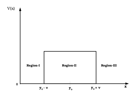
The function $\Theta[x]$ represents the Heaviside step function. In Fig. 6, we give a sketch of the effective potential $V(x)$. In fact, $W_{\nu}(y_{0},x_{0})$ represents the time spent by the particle inside the box, centered around $y_{0}$, till the absorption time $t_{a}$. Hence taking $\nu\to 0$ justifies our construction in Eq. (75) along with Eq. (76).

Figure 6: We have shown the construction of the effective potential $V(x)$ as in Eq. (76) and the disjoint regions as Eq. (76) indicates.

As done in the previous section, we start once again with the generating function $Q_{\nu}(p,y_{0},x_{0})$ of $W_{\nu}(y_{0},x_{0})$ which is defined as

$$Q_{\nu}(p,y_{0},x_{0})=\langle e^{-pW_{\nu}(y_{0},x_{0})}\rangle=\langle e^{-p\int_{0}^{t_{a}}~{}V(x(t))dt}\rangle~{}.$$ (77)

The generating function $\mathcal{T}_{p}(y_{0},x_{0})$ associated to $L_{a}$ is equivalently defined as

$$\mathcal{T}_{p}(y_{0},x_{0})=\langle e^{-pL_{a}(y_{0},x_{0})}\rangle_{x_{0}}=\langle e^{-p\int_{0}^{t_{a}}~{}\delta[x(t)-y_{0}|x_{0}]dt}\rangle~{}.$$ (78)

Both generating functions are related to each other by

$$\mathcal{T}_{p}(y_{0},x_{0})=\lim\limits_{\nu\to 0}Q_{\nu}(p/2\nu,y_{0},x_{0}).$$ (79)

Using the Markov property one can show Majumdar:2005 that, $Q_{\nu}(p,y_{0},x_{0})$ satisfies the following differential equation

$$D\frac{d^{2}Q_{\nu}}{dx_{0}^{2}}-p~{}V(x_{0})~{}Q_{\nu}=0,$$ (80)

which is accompanied by the following boundary conditions : as $x_{0}\to\infty$, the time $t_{a}$ to get absorbed also tends to infinity, which implies that $Q_{\nu}(p,y_{0},x_{0})$ cannot diverge and, secondly, at $x=0$, we have a reactive boundary, which implies that

$$\left[\frac{dQ_{\nu}}{dx_{0}}-\alpha_{0}~{}Q_{\nu}(p,y_{0},x_{0})\right]_{x_{0}=0}=-\alpha_{0}.$$ (81)

The solution of the differential equation Eq. (80) is naturally divided in three different regions: (I) $0\leq x_{0}\leq y_{0}-\nu$, (II) $y_{0}-\nu\leq x_{0}\leq y_{0}+\nu$, and (III) $x_{0}\geq y_{0}+\nu$ (see Fig. 6). The solution can be written in the following way

$$Q_{\nu}(p,y_{0},x_{0}) = A_{\nu}+B_{\nu}~{}x_{0},~{}~{}~{}~{}~{}~{}~{}~{}~{}~{}~{}~{}~{}~{}~{}~{}~{}~{}~{}~{}~{}~{}~{}~{}~{}~{}~{}~{}~{}~{}~{}~{}~{}~{}\text{for}~{}~{}~{}0\leq x_{0}\leq y_{0}-\nu,$$ (82)

$$Q_{\nu}(p,y_{0},x_{0}) = F_{\nu}~{}\cosh\left[(x_{0}-y_{0}-\nu)\sqrt{\frac{p}{D}}~{}\right],~{}~{}~{}~{}\text{for}~{}~{}~{}y_{0}-\nu\leq x_{0}\leq y_{0}+\nu$$ (83)

$$Q_{\nu}(p,y_{0},x_{0}) = F_{\nu},~{}~{}~{}~{}~{}~{}~{}~{}~{}~{}~{}~{}~{}~{}~{}~{}~{}~{}~{}~{}~{}~{}~{}~{}~{}~{}~{}~{}~{}~{}~{}~{}~{}~{}~{}~{}~{}~{}~{}~{}~{}~{}~{}~{}~{}~{}~{}\text{for}~{}~{}~{}x_{0}\geq y_{0}+\nu.$$ (84)

The constants $A_{\nu}$, $B_{\nu}$ and $F_{\nu}$ are computed from the following matching conditions: (a) continuity of the solutions, (b) continuity of their derivatives at $x_{0}=y_{0}\pm\nu$ and (c) using the reactive boundary condition at $x_{0}=0$ according to Eq. (81). Now,

• Using the matching conditions (a) and (b) imply

  $$A_{\nu}+B_{\nu}(y_{0}-\nu)-F_{\nu}~{}\cosh\left[2\nu\sqrt{\frac{p}{D}}~{}\right] = 0,$$ (85)

  $$B_{\nu}(y_{0}-\nu)\sqrt{D}+\sqrt{p}F_{\nu}~{}\sinh\left[2\nu\sqrt{\frac{p}{D}}~{}\right] = 0,$$ (86)

• and using the boundary condition (c) at $x_{0}=0$ we finally obtain

  $$B_{\nu}=\alpha_{0}~{}A_{\nu}-\alpha_{0}.$$ (87)

Solving the three equations (85), (86) and (87), we get

$$A_{\nu}(p) = \alpha_{0}~{}\frac{(y_{0}-\nu)\sqrt{p}\sinh(2\nu\sqrt{p/D})+\sqrt{D}\cosh(2\nu\sqrt{p/D})}{[1+\alpha_{0}(y_{0}-\nu)]\sqrt{p}\sinh(2\nu\sqrt{p/D})+\alpha_{0}\sqrt{D}\cosh(2\nu\sqrt{p/D})},$$ (88)

$$B_{\nu}(p) = -\alpha_{0}~{}\frac{\sqrt{p}\sinh(2\nu\sqrt{p/D})}{[1+\alpha_{0}(y_{0}-\nu)]\sqrt{p}\sinh(2\nu\sqrt{p/D})+\alpha_{0}\sqrt{D}\cosh(2\nu\sqrt{p/D})},$$ (89)

$$F_{\nu}(p) = \frac{\alpha_{0}\sqrt{D}}{[1+\alpha_{0}(y_{0}-\nu)]\sqrt{p}\sinh(2\nu\sqrt{p/D})+\alpha_{0}\sqrt{D}\cosh(2\nu\sqrt{p/D})}.$$ (90)

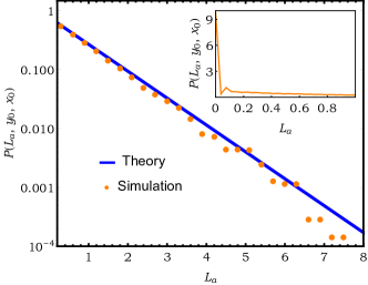
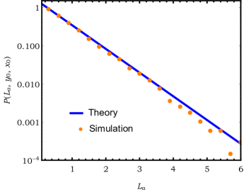
Figure 7: Numerical distribution of the reaction time $P(L_{a},y_{0},x_{0})$ at $y_{0}$ till its first adsorption at $0$ given that it had started from $x_{0}$. We have compared the numerical simulation with the distribution obtained analytically in Eq. (95). The distribution has different analytical forms depending on $x_{0},y_{0}$. In the left panel, we have considered $x_{0}=0.5,y_{0}=0.75$ (so that $x_{0}<y_{0}$) while in the right panel we have $x_{0}=0.75,y_{0}=0.5$ (so that $x_{0}>y_{0}$). In both plots, analytical formulas (solid blue lines) have been plotted against the simulation curves (marked with orange circles). The inset in the left panel shows the presence of the Dirac delta function when $x_{0}<y_{0}$. The parameters for this figure are set as: $D=1,\alpha_{0}=5.0$.

To establish the connection between the generating function as prescribed in Eq. (79), we first take the $\nu\to 0$ limit in the expressions of the constants $A_{\nu}(p/2\nu)$, $B_{\nu}(p/2\nu)$ and $F_{\nu}(p/2\nu)$. This yields

$$A_{a} = \lim\limits_{\nu\to 0}A_{\nu}(p/2\nu)=\frac{\alpha_{0}(y_{0}p+D)}{(1+\alpha_{0}y_{0})p+\alpha_{0}D},$$ (91)

$$B_{a} = \lim\limits_{\nu\to 0}B_{\nu}(p/2\nu)=-\frac{\alpha_{0}p}{(1+\alpha_{0}y_{0})p+\alpha_{0}D},$$ (92)

$$F_{a} = \lim\limits_{\nu\to 0}F_{\nu}(p/2\nu)=\frac{\alpha_{0}D}{(1+\alpha_{0}y_{0})p+\alpha_{0}D}.$$ (93)

All in all, we arrive to the following solution of the generating function $\mathcal{T}_{p}(y_{0},x_{0})$

$$\mathcal{T}_{p}(y_{0},x_{0})=\begin{cases}\frac{p~{}\alpha_{0}(y_{0}-x_{0})+\alpha_{0}D}{(1+\alpha_{0}y_{0})p+\alpha_{0}D},&\text{if~{}~{}}0\leq x_{0}\leq y_{0},\\ \frac{\alpha_{0}D}{(1+\alpha_{0}y_{0})p+\alpha_{0}D},&\text{if~{}~{}}x_{0}\geq y_{0}.\end{cases}$$ (94)

Finally, to obtain the distribution $P(L_{a},y_{0},x_{0})$ we need to perform the inverse Laplace transform in Eq. (94) , which yields the full distribution of the reaction time profile

$$P(L_{a},y_{0},x_{0})=\begin{cases}\frac{2\alpha_{0}(y_{0}-x_{0})}{1+\alpha_{0}y_{0}}~{}\delta(L_{a})+\alpha_{0}D~{}\frac{1+\alpha_{0}x_{0}}{(1+\alpha_{0}y_{0})^{2}}~{}e^{-\frac{\alpha_{0}D}{1+\alpha_{0}y_{0}}~{}L_{a}},&\text{if~{}~{}}0\leq x_{0}\leq y_{0},\\ \frac{\alpha_{0}D}{(1+\alpha_{0}y_{0})}~{}e^{-\frac{\alpha_{0}D}{1+\alpha_{0}y_{0}}~{}L_{a}},&\text{if~{}~{}}x_{0}\geq y_{0}.\end{cases}$$ (95)

In the above expression we see that there is a $\delta$-function contribution to the distribution of $L_{a}$. This results from those paths which are absorbed at the boundary before making a first passage to $y_{0}$. For this reason, the $\delta$-function contribution appears only when $0\leq x_{0}\leq y_{0}$ or, in other words, there is a chance for the molecule to be absorbed at the boundary at $x=0$ before ever reaching $y_{0}$ for the first time. This element of chance decreases as one starts closer to $y_{0}$, which explains the multiplicative factor $(y_{0}-x_{0})$. One the other hand, if the molecule starts at $x_{0}\geq y_{0}$ it will definitely cross $y_{0}$ before it is absorbed at $x=0$ and, as a result, it spends some time around $y_{0}$ (due to the Brownian nature of the motion). This is the reason behind the absence of a $\delta$-function term for $x_{0}\geq y_{0}$. In Fig. 7 we compare the analytical expression given by Eq. (95) to simulation results finding, once again, an excellent agreement.

IV Methods of simulations

In this section, we outline the method we have used to simulate our system. There are many ways to generate trajectories of a Brownian particle diffusing in a box with two reactive boundaries Singer08 ; Erban07 ; Andrews-2009 ; Bray-2004 . In one such method, as described in Singer08 , the authors define the partially reflected process as the limit of a Markovian jump process generated by the dynamics using an Euler scheme. Using boundary layer analysis, they derive a relation between the reactive constants and the reflection probability. In another paper Erban07 , the authors study four different approaches to simulate such systems and they have derived the correct choices of the reactive boundary conditions to implement in stochastic simulations. In this paper, we have adapted one of these approaches from Erban07 to generate the trajectories. This is known as the Euler scheme for velocity jump process Erban07 . In this scheme, one simulates the system by defining an auxiliary underdamped motion (by introducing a velocity component along with the existing position component) with friction coefficient $\Gamma$. The dynamics is discrete in time, continuous in space and discontinuous in velocities. We sketch the basic steps in the following lines.

Let us consider a system of $N$ independent molecules (i.e., N independent and identical copies of the system). The $i$-th molecule is described by two variables: its position $x_{i}(t)$ and velocity $v_{i}(t)$ at time $t$. The underdamped dynamics for the set $\{x_{i}(t),v_{i}(t)\}$ at each time step $\Delta t$ is introduced in the following way:

$$x_{i}(t+\Delta t) = x_{i}(t)+v_{i}(t)\Delta t,$$

$$v_{i}(t+\Delta t) = v_{i}(t)-\Gamma v_{i}(t)\Delta t+\Gamma~{}\sqrt{2D\Delta t}~{}\eta_{i},$$ (96)

where $\Gamma$ should be taken large and $\eta_{i}$ is a normally distributed random variable with zero mean and unit variance Erban07 . In this problem we have two reactive boundaries at $x=0$ and $x=L$ and the reactive boundary conditions can be stated as follows: whenever a molecule hits any one of the two boundaries ($0,L$) it is adsorbed with probability $p_{0}/\sqrt{\Gamma}$ or $p_{L}/\sqrt{\Gamma}$ respectively, or reflected otherwise. The implementation is the following: whenever the value $x_{i}(t+\Delta t)$ computed from Eq. (96) is negative then

$$x_{i}(t+\Delta t) = -x_{i}(t)-v_{i}(t)\Delta t,$$

$$v_{i}(t+\Delta t) = -v_{i}(t)+\Gamma v_{i}(t)\Delta t-\Gamma~{}\sqrt{2D\Delta t}~{}\eta_{i},$$ (97)

with probability $1-\frac{p_{0}}{\sqrt{\Gamma}}$, or we remove the $i$-th molecule from the system. On the other hand, if $x_{i}(t+\Delta t)$ computed from Eq. (96) is greater than $L$, we do the following

$$x_{i}(t+\Delta t) = 2L-x_{i}(t)-v_{i}(t)\Delta t,$$

$$v_{i}(t+\Delta t) = -v_{i}(t)+\Gamma v_{i}(t)\Delta t-\Gamma~{}\sqrt{2D\Delta t}~{}\eta_{i},$$ (98)

with probability $1-\frac{p_{L}}{\sqrt{\Gamma}}$, otherwise we remove the $i$-th molecule from the system. Finally, we use the following relation between the reactive constants and the reflection probabilities Erban07

$$p_{0} = \frac{\alpha_{0}\sqrt{2\pi}}{\sqrt{D}}$$

$$p_{L} = \frac{\alpha_{L}\sqrt{2\pi}}{\sqrt{D}}.$$ (99)

It is important that only in the high friction limit, that is, only when $\Gamma$ is large enough, we recover the diffusion equation Eq. (1) which is the overdamped limit and the inception of our study. The above prescription allows us to successfully generate Brownian trajectories in the presence of two reactive boundaries and the number of molecules present in the system after a given time $t$ is simply proportional to the probability density defined in Eq. (1). We conclude this section by stating that other statistical quantities such as the survival probability or the reaction time profile can be also simulated using this method.

V Conclusions and Future Outlook

In this paper, we have built a comprehensive theory to study various statistical properties of a Brownian molecule in presence of reactive boundaries. Such boundaries are ubiquitous in physics, chemistry and biology. Several molecular movements inside a cell can fairly well be described by a Brownian motion where the cell boundary provides the confined geometry. One often considers these boundaries to be either completely reflecting or completely absorbing. However, the effects of adsorption, catalysis etc. occurring at the cell boundary makes them reactive, in the sense that these boundaries are neither fully absorbing nor fully reflecting. In this paper, we have looked at the Brownian motion of a molecule in one dimension with partially absorbing (reflecting) boundaries. In this case, we find that the propagator of the molecule is different from that with fully absorbing/reflecting boundaries. We have also looked at the survival properties of the molecule, which also provides explicit expressions of the distribution of absorption time, the mean absorption time as well as the distribution of the maximum displacement. Using the Feynman-Kac formalism, we have investigated the distribution of the reaction or local time density both when observed for a fixed time or till the absorption time. We have obtained explicit expressions of the distribution of the reaction time which give an excellent match with the numerical simulations.

Our work can be extended in multiple directions. In a recent study Grebenkov-17-target , the authors considered the mean first passage time to a reaction event on a specific site in a cylindrical geometry with mixed boundary conditions. It would be interesting to estimate the survival probabilities and the longest excursions (maximum displacement and time to reach the maximum) in such set up and further extend it to different non-uniform geometries. It would be also interesting to see how the properties of a tagged particle in presence of other particles are effected by considering reactive crossing conditions. Effects of a partially absorbing boundary have also been investigated recently in an interesting stochastic dynamics namely stochastic resetting EM11a ; EM11b ; KMSS14 ; Pal14 which mixes long range moves along with the local moves due to diffusion Whitehouse-Martin-Satya . Moreover, such dynamics could be quite benifical strategies to target search SR2016 ; AAM16 ; PalShlomi2016 . It is left for future studies to combine this dynamics in conjugation with diffusion to expedite first passage processes to a target in a confined domain with reactive boundaries.

VI Acknowledgment

Arnab Pal gratefully acknowledges support from the Raymond and Beverly Sackler Post-Doctoral Scholarship at Tel-Aviv University. Anupam Kundu acknowledges support from DST grant under project No. ECR/2017/000634. This work benefited from the support of the project 5604-2 of the Indo-French Centre for the Promotion of Advanced Research (IFCPAR). We would also like to thank the Weizmann Institute of Science for the hospitality during the SRitp workshop where part of this work was done. Isaac Pérez Castillo thanks hospitality of the Laboratoire de Physique Théorique et Modèles Statistiques (Université de Paris-Sud), where this work was initiated.

VII Appendix

VII.1 Derivations of propagator in semi-infinite domain

To derive the propagator in the semi-infinite domain, we have to take the limit $L\to\infty$ in Eq. (22). In this limit Eq. (17) yields $k=\frac{n\pi}{L}$. The summation over $k$ can now be converted into an integral over $k$ as $L\to\infty$. A short calculation gives us

$$G_{t}^{\text{si}}(x,x_{0}) =\frac{1}{2\pi}~{}\left[\frac{\partial}{\partial x}\frac{\partial}{\partial x_{0}}+\alpha_{0}\left(\frac{\partial}{\partial x}+\frac{\partial}{\partial x_{0}}\right)+\alpha_{0}^{2}\right]\int_{-\infty}^{\infty}~{}dk~{}\frac{2\sin(kx_{0})\sin(kx)}{\alpha_{0}^{2}+k^{2}}~{}e^{-Dk^{2}t}$$

$$=\frac{1}{2\pi}~{}\Big{(}\frac{\partial}{\partial x}+\alpha_{0}\Big{)}\Big{(}\frac{\partial}{\partial x_{0}}+\alpha_{0}\Big{)}\int_{-\infty}^{\infty}~{}dk~{}\frac{\cos[k(x+x_{0})]+\cos[k(x-x_{0})]}{\alpha_{0}^{2}+k^{2}}~{}e^{-Dk^{2}t}\,.$$ (100)

To compute Eq. (100) we consider the following integral

$$I_{\alpha}(z) = \int_{-\infty}^{\infty}~{}dk~{}\frac{\cos(kz)}{\alpha^{2}+k^{2}}~{}e^{-k^{2}t}$$ (101)

$$= e^{\alpha^{2}t}\left[\int_{-\infty}^{\infty}~{}dk~{}\frac{\cos(kz)}{\alpha^{2}+k^{2}}~{}e^{-(\alpha^{2}+k^{2})t}\right]\,.$$

By noting that $\int_{t}^{\infty}~{}dt^{\prime}~{}e^{-(k^{2}+\alpha^{2})t^{\prime}}=\frac{e^{-(\alpha^{2}+k^{2})t}}{\alpha^{2}+k^{2}}$, we find from Eq. (101)

$$I_{\alpha}(z) = e^{\alpha^{2}t}~{}\int_{t}^{\infty}~{}dt^{\prime}~{}e^{-\alpha^{2}t^{\prime}}~{}\text{Re}\left[\int_{-\infty}^{\infty}~{}dk~{}e^{ikz}~{}e^{-k^{2}t^{\prime}}\right]$$ (102)

$$= \frac{2\sqrt{\pi}}{\alpha}~{}e^{y^{2}}~{}\int_{y}^{\infty}~{}dq~{}e^{-q^{2}}~{}e^{-\frac{z^{2}\alpha^{2}}{4q^{2}}}\,,$$

where $y=\alpha\sqrt{t}$. Applying the following standard integral formula

$$\int_{y}^{\infty}~{}dt~{}e^{-a^{2}t^{2}-\frac{b^{2}}{t^{2}}}=\frac{\sqrt{\pi}}{4a}~{}e^{2ab}~{}\mathrm{erfc}\left[ay+\frac{b}{y}\right]+\frac{\sqrt{\pi}}{4a}~{}e^{-2ab}~{}\mathrm{erfc}\left[ay-\frac{b}{y}\right]\,,$$ (103)

in Eq. (102), eventually we obtain from Eq. (101)

$$I_{\alpha}(z)=\frac{\pi}{2\alpha}e^{\alpha^{2}t}~{}\left[e^{z\alpha}~{}\mathrm{erfc}\left(\frac{2\alpha t+z}{\sqrt{4t}}\right)+e^{-x_{0}\alpha}~{}\mathrm{erfc}\left(\frac{2\alpha t-z}{\sqrt{4t}}\right)\right]\,.$$ (104)

Plugging the above expression in Eq. (100), we obtain Eq. (23) as mentioned in the main text along with Eq. (24).

References

• (1) H. Berg, Random Walks in Biology (Princeton: Princeton University Press) (1983).
• (2) J. Crank, The Mathematics of Diffusion (Oxford: Oxford University Press) (1975).
• (3) G. M. Cooper and R. E. Hausman, The Cell: A Molecular Approach, (Seventh Edition: Sinauer Associates) (2016).
• (4) L. Vroman, A. L. Adams, G. C. Fischer, and P. C. Munoz, Blood 55, 156 (1980); J. L. Brash et al., ibid. 71, 932 (1988); J. G. Donaldson, R. A. Kahn, J. Lippincott-schwartz, and R. D. Klausner, Science 254, 1197 (1991).
• (5) O. V. Bychuk and B. O. Shaughnessy, Phys. Rev. Lett. 74, 1795 (1995); R. Valiullin, R. Kimmich, and N. Fatkullin, Phys. Rev. E 56, 4371 (1997).
• (6) D. S. Grebenkov, in Focus on Probability Theory, Ed. L. R. Velle, pp. 135-169 (Nova Science Publishers) (2006).
• (7) D. S. Grebenkov, Rev. Mod. Phys. 79, 1077 (2007).
• (8) R. Zwanzig, Proc. Nati. Acad. Sci. USA, 87, 5856-5857, (1990).
• (9) S. A. Allison, S. H. Northrup, and J. A. McCammon, The Journal of Chemical Physics 83, 2894 (1985).
• (10) G. Lamm and K. Schulten, The Journal of Chemical Physics 78, 2713 (1983).
• (11) S. J. Chapman, R. Erban, and S. A. Isaacson, Siam J. Appl. Math., 76(1), 368-390 (2016).
• (12) R. Erban and S. J. Chapman, Phys. Biol. 4, 16-28 (2007).
• (13) J. Hattne, D. Fagne and J. Elf, Bioinformatics 21, 2923-4 (2005).
• (14) K. Naqvi, K. Mork, and S. Waldenstrom, Phys. Rev. Lett. 49, 304-7 (1982).
• (15) E. Jacob, Stochastic Processes and their Applications, 122(1), pp.191-216 (2012).
• (16) M. A El-Shehawey, Journal of Physics A: Mathematical and General 33, 49, 9005 (2000).
• (17) F. C. Goodrich, Journal of Chemical Physics, 22 588-594, (1954).
• (18) D. S. Grebenkov, Journal of Physics A: Mathematical and Theoretical 48, 1, 013001 (2014).
• (19) J. S.Vrentas, C.M. Vrentas , Chem. Eng. Sci., 44(12), 3001 - 3003 (1989).
• (20) I. P. Castillo and T. Dupic, J. Stat. Phys. 156, 606 (2014).
• (21) P. H. von Hippel and O. G. Berg, J. Biol. Chem. 264, 675 (1989), and references therein.
• (22) M. Slutsky and L. A. Mirny, Biophys. J. 87, 4021 (2004); M. Coppey, O. Benichou, R. Voituriez, and M. Moreau, Biophys. J. 87, 1640 (2004); I. M. Sokolov, R. Metzler, K. Pant, and M. C. Williams, Biophys. J. 89, 895 (2005); Y. M. Wang, R. H. Austin, and E. C. Cox, Phys. Rev. Lett. 97, 048302 (2006).
• (23) D. S. Grebenkov, Phys. Rev. E 91, 052108 (2015).
• (24) R. Dickman and D. ben-Avraham, Phys. Rev. E 64, 020102(R) (2001).
• (25) A. V. Skorokhod, Siam Theory Probab. Appl., 6 (3), 264-274. (1959); ibid. 7 (1), 3-23 (1959).
• (26) K. Burdzy, Z.Q. Chen, and J. Sylvester, Ann. Probab., 32, 1B , 775-804 (2004).
• (27) A. Singer, Z. Schuss, A. Osipov, and D. Holcman, SIAM J. Appl. Math., 68 (3), 844-868 (2008).
• (28) L. Batsilas, A. M. Berezhkovskii, and S. Y. Shvartsman, Biophys. J., 85 , 3659-3665 (2003).
• (29) A. M. Berezhkovskii, Y. A. Makhnovskii, M. I. Monine, V. Yu. Zitserman, and S. Y. Shvartsman, J. Chem. Phys., 121, 11390-11394 (2004).
• (30) M. I. Monine and J. M. Haugh, J. Chem. Phys., 123 , 074908 (2005).
• (31) M. A. Lomholt, I. M. Zaid, and R. Metzler, Phys. Rev. Lett. 98, 200603 (2007).
• (32) S. Stapf, R. Kimmich, and R. O. Seitter, Phys. Rev.Lett. 75, 2855 (1995); P. Levitz et al., ibid. 96, 180601 (2006).
• (33) B. Sapoval, Phys. Rev. Lett. 73, 3314 (1994).
• (34) A. A. Sonin, A. Bonfillon, and D. Langevin, Phys. Rev. Lett. 71, 2342 (1993); C. Stenvot and D. Langevin, Langmuir 4, 1179 (1988).
• (35) E. R. Weibel, The Pathway for oxygen. Structure and function in the mammalian respiratory system (Harvard University Press, Cambridge, Massachusetts and London, England) (1984).
• (36) B. Mauroy, M. Filoche, E. R. Weibel, and B. Sapoval, Nature 427, 633 (2004).
• (37) B. Sapoval, M. Filoche, and E. R. Weibel, Branched Structures, Acinus Morphology and Optimal Design of Mammalian Lungs, in Branching in nature, Eds. by V. Fleury, J.-F. Gouyet, and M. Leonetti, 225-242 (EDP Sciences/Springer Verlag) (2001).
• (38) B. Sapoval, J. S. Andrade Jr., and M. Filoche, Chem. Eng. Sci. 56, 5011 (2001).
• (39) J. S. Andrade Jr., M. Filoche, and B. Sapoval, Europhys. Lett. 55, 573 (2001).
• (40) J. S. Andrade Jr., H. F. da Silva, M. Baquil, and B. Sapoval, Phys. Rev. E 68, 041608 (2003).
• (41) A. J. Bray, S. N. Majumdar, and G. Schehr, Advances in Physics 62, 225 (2013).
• (42) S. N. Majumdar, Curr. Sci. 89, 2076 (2005).
• (43) S. Redner, A guide to First-Passage Processes, (Cambridge University Press, Cambridge), (2001).
• (44) R. Metzler, G. Oshanin, S. Redner Ed., First-Passage Phenomena and Their Applications, (World Scientific) (2014).
• (45) O. Bénichou, C Loverdo, M. Moreau, and R. Voituriez, Rev. Mod. Phys. 83 81 2011.
• (46) D. S. Grebenkov and J.-F. Rupprecht, The Journal of Chemical Physics 146, 084106 (2017).
• (47) P. Salminen, and M. Yor, Periodica Mathematica Hungarica, 62, 1, 75-101 (2011).
• (48) E. Ben-Naim, S. Redner and G. H. Weiss, J. Stat. Phys. 71, 75 (1993).
• (49) J. Whitehouse, M. R. Evans, and S. N. Majumdar, Phys. Rev. E 87, 022118 (2013).
• (50) H. Sano and M. Tachiya, The Journal of Chemical Physics 71, 1276 (1979).
• (51) L. Menten and M. I. Michaelis, Biochemische Zeitschrift 49, 333 (1913).
• (52) S. Sabhapandit, S. N. Majumdar, and A. Comtet, Phys. Rev. E 73, 051102 (2006).
• (53) M. D. Donsker and S. R. S. Varadhan, I, Commun. Pure Appl. Math. 28, 1 (1975).
• (54) A. C. Barato and R. Chetrite, J. Stat. Phys. 160, 1154 (2015).
• (55) P. L. Krapivsky, S. N. Majumdar, A. Rosso, J. Phys. A: Math. Theor. 43, 315001 (2010).
• (56) S. S. Andrews, Physical Biology, 6(4):046015, (2009).
• (57) S. S. Andrews and D. Bray, Physical biology, 1 (3), p.137 (2004).
• (58) D. S. Grebenkov, R Metzler, G Oshanin, New Journal of Physics 19 (10), 103025 (2017).
• (59) M. R. Evans, and S. N. Majumdar, Phys. Rev. Lett. 106, 160601 (2011).
• (60) M. R. Evans, and S. N. Majumdar, J. Phys. A: Math. Theor. 44, 435001 (2011).
• (61) L. Kusmierz, S. N. Majumdar, S. Sabhapandit, and G. Schehr, Phys. Rev. Lett. 113, 220602 (2014).
• (62) A. Pal, Phys. Rev. E 91, 012113 (2015).
• (63) S. Reuveni, Phys. Rev. Lett. 116, 170601 (2016).
• (64) A. Pal, A. Kundu and M. R. Evans, J. Phys. A: Math. Theor. 49, 225001 (2016).
• (65) A. Pal, and S. Reuveni, Phys. Rev. Lett. 118, 030603 (2017).