Improving Predictive Uncertainty Estimation using Dropout - Hamiltonian Monte Carlo

Abstract

Estimating predictive uncertainty is crucial for many computer vision tasks, from image classification to autonomous driving systems. Hamiltonian Monte Carlo (HMC) is an sampling method for performing Bayesian inference. On the other hand, Dropout regularization has been proposed as an approximate model averaging technique that tends to improve generalization in large scale models such as deep neural networks. Although, HMC provides convergence guarantees for most standard Bayesian models, it does not handle discrete parameters arising from Dropout regularization. In this paper, we present a robust methodology for improving predictive uncertainty in classification problems, based on Dropout and Hamiltonian Monte Carlo. Even though Dropout induces a non-smooth energy function with no such convergence guarantees, the resulting discretization of the Hamiltonian proves empirical success. The proposed method allows to effectively estimate the predictive accuracy and to provide better generalization for difficult test examples.

1 Introduction

Artificial Intelligence systems have a wide variety of applications and in some cases are part of complex systems whose operation involves making delicate and dangerous decisionsLeibig et al. [2017]. Uncertainty in knowledge representation and reasoning has been studied since the fall of symbolic expert systems Pearl [1988]. Therefore, several research efforts focused on efficient methods for estimating model uncertainty and capturing the variability inherent to real world situations Bishop [2007].

Inference using uncertainty estimates is crucial for many important tasks, such as image classification, detecting noisy examples (adversarial examples) and analyzing failure cases in decision-making systems Prince [2012]. These problems can benefit on predictive uncertainty for achieving good performance, requiring well calibrated probabilities. In such cases, Bayesian inference provides posterior predictive distributions that can be used to reduce over-confidence of the model outputs Gelman et al. [2014].

Bayesian neural networks consider model weights as random variables and have been proposed as a method to estimate predictive uncertainty Neal [2012], however inference is computationally intractable for deep neural networks. More recently, Gal and Ghahramani [2016] proposed Monte Carlo Dropout as a method to obtain uncertainty estimates from deep learning architectures. Dropout has been previously proposed as a regularization technique for deep neural networks (see Srivastava et al. [2014]) and the relationship with Bayesian model uncertainty being justified as a variational approximation. The key idea is to train a deep learning model and perform inference using Monte Carlo and dropout in order to obtain an approximate posterior distribution.

Hamiltonian Monte Carlo (HMC) is a Markov Chain Monte Carlo (MCMC) method for obtaining a sequence of random samples while maintaining asymptotic consistency with respect to a target distribution Neal et al. [2011]. HMC provides a mechanism for defining proposals with high acceptance rate, enabling more efficient exploration of the state space than standard random-walk proposals. In addition, another property of HMC is the feasibility to support high dimensional models arising from deep neural architectures Beskos et al. [2013].

Although HMC was originally proposed for training Bayesian neural networks, the method is not well suited for discrete parameters arising from dropout layers. In this work, we propose a methodology named Dropout - Hamiltonian Monte Carlo (D-HMC). The proposed approach is tested with the MNIST digit recognition LeCun et al. [1998] and predictive uncertainty is compared to other sampling approaches such as Stochastic Gradient HMC (SGHMC) Chen et al. [2014] and Stochastic Gradient Langevin Dynamics (SGLD) Welling and Teh [2011].

Transfer learning is a popular approach for domain adaption, when a large amount of data is used to pre-train a deep neural network and only a smaller amount of data is available for the new task Li and Hoiem [2018]. The new model is prone to over-fitting, therefore a careful choice of the hyper-parameters used for transfer learning must be carried out in order to preserve the performance of the original task Miceli Barone et al. [2017]. Conversely, we develop a novel methodology to represent predictive uncertainty when using convolutional neural networks for transfer learning for age recognition Eidinger et al. [2014].

2 Related Work

HMC relies on a numerical approximation (an integrator) of a continuous dynamical system. The method is designed in a way that the main properties of the dynamical system are preserved. However, the approximation error is highly sensitive to critical user-specified hyper-parameters, such as the number of steps and the step size. Hoffman et. al. introduced the No-U-Turn sampler (NUTS) Hoffman and Gelman [2014], as a method to determine the appropriate number of steps that the algorithm needs in order to converge to the target distribution. This method uses a recursive algorithm to build a set of likely candidate points, stopping automatically when it starts to double back and retrace its steps. In practice, simple heuristics can also be used to establish the number of steps and the step size, based on the assumption that the posterior distribution is Gaussian with diagonal covariance Hoffman [2017].

Other highly successful implementations focus on tackling large data sets using ideas from stochastic optimization such as Stochastic Gradient Descent (SGD). The SGHMC and SGLD techniques support data batches and introduces a novel integrator using Langevin dynamics which takes into account the extra-noise induced in the gradient Chen et al. [2014], Welling and Teh [2011]. Another technique, the Metropolis Adjusted Langevin Algorithm (MALA) Roberts and Rosenthal [1998], Roberts and Stramer [2002], uses a Metropolis-Hastings (Metropolis) correction scheme to accept or reject proposals. Also, the Riemann Manifold Hamiltonian Monte Carlo method provides better adaption to the problem geometry for strongly correlated densities (RMHMC) Girolami and Calderhead [2011], Wang et al. [2013]. Finally, proximal algorithms and convex optimization techniques have also been studied in the context of MCMC Pereyra [2016], and HMC with log-concave or non-differentiable (non-smooth) energy functions Chaari et al. [2016].

3 Methods

Different architectures have been proposed for image classification using deep neural networks. However, most models have a fully connected layer that compares the network output $\mathbf{x}$ with the sample training label $y$. Conversely, an image dataset $\mathbf{D}=\{\mathbf{d_{1}},\ldots,\mathbf{d_{N}}\}$ can be represented by a set of tuples $d=(\mathbf{x},y)$ that contains the image features $\mathbf{x}\in\mathbb{R}^{D}$ and the labels $y=\{1,\ldots,K\}$. The fully connected layer consists of an activation function such as the softmax, which encodes the image features into a vector of class probabilities $[\phi_{1}(\theta),\ldots,\phi_{k}(\theta)]$, whose elements can be written as:

$$\phi_{i}(\theta)=\frac{\operatorname{exp}(\mathbf{x}^{T}\mathbf{w_{i}}+b_{i})}{\sum\limits_{k=1}^{K}\operatorname{exp}(\mathbf{x}^{T}\mathbf{w_{k}}+b_{k})}$$ (1)

where $\theta=\{(\mathbf{w}_{1},\mathbf{b}_{1}),\ldots,(\mathbf{w}_{K},\mathbf{b}_{K})\}$, $\mathbf{w}_{i}\in\mathbb{R}^{D}$ is a vector, $b_{i}$ is an scalar, $D$ represents the dimensionality of the feature space $\mathbf{x}$ and $K$ the number of classes.

3.1 Hamiltonian Monte Carlo

Now, we consider the unknown parameter $\theta$ as a random variable. In a Bayesian setting, we want to sample from the posterior distribution $p(\theta|\mathbf{D})$ given by:

$$p(\theta|\mathbf{D})=\frac{p(\mathbf{D}|\theta)p(\theta)}{p(\mathbf{D})} =\frac{p(\mathbf{D}|\theta)p(\theta)}{\int p(\mathbf{D}|\theta)p(\theta)\,d\theta}$$ (2)

$$\propto p(\mathbf{D}|\theta)p(\theta)$$ (3)

The target distribution $p(\theta|\mathbf{D})$ is known up to a normalization constant. Standard Markov Chain Monte Carlo methods such as the Metropolis-Hastings algorithm can be used to obtain the required posterior probabilities Gelman et al. [2014]. However due to the complexity of the target distribution (e.g. high-dimensional and possibly correlated image features),the algorithm would perform an inefficient exploration of the posterior. Instead, HMC improves the exploration by simulating Hamiltonian dynamics. A Hamiltonian function $H$ is composed as a potential energy $U$ and a kinetic energy $K$. These terms are constructed as follows:

$$H(\theta,r)=U(\theta)+K(r)$$ (4)

where $r$ is called the momentum and is considered as an auxiliary variable. A positive-definite mass matrix $M$ is also introduced as follow:

$$U(\theta) =-\sum_{d\in\mathbf{D}}\log p(d|\theta)-\log p(\theta)$$ (5)

$$K(r) =\frac{1}{2}r^{T}M^{-1}r$$ (6)

For image classification problems, the density $p(d|\theta)=\prod_{i=1}^{K}\phi_{i}(\theta)^{[y=k]}$ takes the form of a categorical distribution over the $K$ different classes and the prior $p(\theta)\sim\mathcal{N}(0,\alpha\mathbf{I}_{D})$ takes the form of a multivariate Gaussian distribution. Now, in order to sample from $p(\theta|\mathbf{D})$, the method simulates Hamiltonian dynamics while leaving the joint distribution $(\theta,r)$ invariant, such that:

$$p(\theta|\mathbf{D}) \propto\exp(-U(\theta))$$ (7)

$$\pi(\theta,r) \propto\exp(-H(\theta,r))$$ (8)

The first step proposes a new value for the momentum variable from a Gaussian distribution. Then, a Metropolis update using Hamiltonian dynamics is used to propose a new state. The state evolves in a fictitious continuous time $t$, and the partial derivatives of the Hamiltonian can be seen in Equation 10.

$$d\theta =M^{-1}r\,dt$$ (9)

$$dr =-\nabla U(\theta)\,dt$$ (10)

In order to simulate continuous dynamics, the leapfrog integrator can be used to discretize time. Using a small step size $\epsilon$, Equation 10 becomes:

$$r_{i}^{(t+\frac{\epsilon}{2})} =r_{i}^{(t)}-\frac{\epsilon}{2}\nabla U(\theta^{(t)})$$ (11)

$$\theta_{i}^{(t+\epsilon)} =\theta_{i}^{(t)}+\epsilon r^{(t+\frac{\epsilon}{2})}M_{i}^{-1}$$ (12)

$$r_{i}^{(t+\epsilon)} =r_{i}^{(t+\frac{\epsilon}{2})}-\frac{\epsilon}{2}\nabla U(\theta^{(t+\epsilon)})$$ (13)

After $i=1,\ldots,m$ iterations of the leapfrog integrator with finite $\epsilon$, the joint proposal becomes $(\theta^{(t+1)},r^{(t+1)})=(\theta_{m},r_{m})$. Subsequently, a Metropolis update is used to accept the proposal with probability $\rho>\operatorname{unif}(0,1)$, such that:

$$\centering\begin{split}\rho=&\min\{1,\exp(-H(\theta^{(t+1)},r^{(t+1)}))+H(\theta^{(t)},r^{(t)})\}\end{split}\@add@centering$$ (14)

3.1.1 Properties of Hamiltonian dynamics

An integrator is an algorithm that numerically approximates an evolution of the exact solution of a differential equation. Some important properties of Hamiltonian dynamics are important for building MCMC updates Neal et al. [2011]:

• Reversibility: The dynamics are time-reversible.

• Volume Preservation: Hamiltonian dynamics are volume preserving.

• Conservation of the Hamiltonian: $H$ is constant as $\theta$ and $r$ vary.

The leapfrog method in HMC satisfies the criteria of volume conservation and reversibility over time. However, the total energy is only conserved approximately, in this way a bias is introduced in the joint density $\pi(\theta,r)$. Conversely, the Metropolis update is used to satisfy the detailed balance condition.

3.1.2 Limitations of HMC

One of the main limitations of HMC is the lack of support for discrete parameters. The difficulty in extending HMC to a discrete parameter space stems from the fact that the construction of proposals relies on the numerical solution of a differential equation. In other hand, approximating the likelihood of a discrete parameter by a continuous density is not always possible Nishimura et al. [2017]. Moreover, when any discontinuity is introduced into the energy function ($U(\theta)$), the first-order discretization does not ensure that a Metropolis correction maintains the stationary distribution invariant. Therefore, the standard implementation of HMC does not guarantee convergence when the parameter of interest has a discontinuous density. This is because integrators are designed for differential equations with smooth derivatives over time.

3.2 Dropout / DropConnect

Dropout and DropConnect arise in the context regularization of deep neural networks and provide a way to combine exponentially many different architectures Srivastava et al. [2014], Wan et al. [2013]. Dropout/DropConnect can be described as follows:

• Regular (binary) DropConnect adds noise to global network weights, by setting a randomly selected subset of weights to zero computed by element-wise multiplication of a binary mask $\Gamma$:

  $$\phi_{c,i}(\theta,\Gamma)=\frac{\operatorname{exp}(\mathbf{x}^{T}(\Gamma\odot\mathbf{w_{i}})+b_{i})}{\sum\limits_{k=1}^{K}\operatorname{exp}(\mathbf{x}^{T}(\Gamma\odot\mathbf{w_{k}})+b_{k})}$$ (15)

• Instead, binary Dropout randomly selects local inputs:

  $$\phi_{d,i}(\theta,\Gamma)=\frac{\operatorname{exp}((\Gamma\odot\mathbf{x}^{T})\mathbf{w_{i}}+b_{i})}{\sum\limits_{k=1}^{K}\operatorname{exp}((\Gamma\odot\mathbf{x}^{T})\mathbf{w_{k}}+b_{k})}$$ (16)

where $\Gamma\sim\mathcal{B}(1-p)$ is a Bernoulli distributed random mask and $p$ is the probability that the weight/input being dropped.

Due to its great effectiveness in various types of neural networks, the Dropout learning scheme has been the subject of research in recent years. Thus, it has been shown that Dropout is similar to bagging and other related ensemble methods Warde-Farley et al. [2013]. Since all models are averaged in a efficient and fast approximation with weights scaling, Dropout can be seen as an approximation to the geometric mean in the space of all possible models, this approximation is less expensive than the arithmetic mean in bagging methods Baldi and Sadowski [2013].

4 Dropout - Hamiltonian Monte Carlo

Stochastic gradient descent optimization has been extensively used for training neural networks. Instead of using the gradient of the full likelihood, stochastic gradients are used to update model parameters. In the context of Bayesian models, SGLD combines noisy gradient updates with Langevin dynamics in order to generate proposals from data subsets $B_{i}\subset\mathbf{D}$ such that:

$$\tilde{U}(\theta)=-\frac{N}{n}\sum_{d\in B_{i}}\log p(d|\theta,\Gamma)-\log p(\theta)$$ (17)

where $i=1,\ldots,N$, $N$ is the number of data subsets and $n=|B_{i}|$ the size of the mini-batch and $p$ the dropout rate.

Chen et.al. introduce a new momentum variable $\nu$ as an alternative discretization for HMC Chen et al. [2014]. Similar to SGLD, the choice of the step size must balance between efficient sampling and high acceptance rates (speed and accuracy). Equation 18 shows the SGHMC update.

$$\theta^{(t+1)} =\theta^{(t)}+\nu^{(t)}$$ (18a)

$$\nu^{(t+1)} =(1-\alpha)\nu^{(t)}+\epsilon\nabla\tilde{U}(\theta^{(t+1)})+\xi^{(t)}$$ (18b)

$$\xi^{(t)} =\mathcal{N}(0,2[\alpha-\beta]\epsilon)$$ (18c)

where $\mathcal{N}$ denotes a multivariate normal density, $v$ denotes the momentum variable in SGHMC, $\epsilon$ denotes the step size, while $\alpha$ and $\beta$ are tuning constants.

Integrating Dropout into SGHMC can be seen as adding a regularization term. Since HMC cannot perform inference on the discrete parameters, the gradient can be computed by either marginalization or by means of a local reparameterization Kingma et al. [2015]. Therefore, on each iteration a multivariate Bernoulli mask $\Gamma\sim\mathcal{B}(1-p)$ with probability $1-p$ is applied to the $\theta$ parameter and then to the gradient of the energy function $\tilde{U}(\theta)$. Conversely, the density $p(d|\theta,\Gamma)=\prod_{i=1}^{K}\phi_{d,i}(\theta,\Gamma)^{[y=k]}$ takes the form of a modified categorical distribution. Each one of the input components is randomly deleted and the remaining elements are scaled up by $1/p$. The noisy gradient updates generate proposals from a perturbed target distribution Bardenet et al. [2014]. The proposed method is described in algorithm 1.

Algorithm 1 D-SGHMC

0:  $\theta_{\ast},M,p,\alpha,\beta,\epsilon$.

  $v_{\ast}\sim\mathcal{N}(0,M)$

  $(\theta_{0},v_{0})=(\theta_{\ast},v_{\ast})$

  for $t=1,2,\ldots$ do

     Sample dropout mask $\Gamma$

     $\Gamma\sim\mathcal{B}(1-p)$

     Transform mini-batch $B_{t}$ using binary mask

     $B_{t}^{\prime}\leftarrow 1/p\,(\Gamma\odot B_{t})$

     $(\theta^{0},v^{0})=(\theta_{t-1},v_{t-1})$

     for $i=1,2,\ldots,L$ do

        $\theta^{i}\leftarrow\theta^{i-1}+v^{i-1}$

        $v^{i}\leftarrow(1-\alpha)v^{i-1}+\epsilon\nabla\tilde{U}(\theta^{i})+\mathcal{N}(0,2[\alpha-\beta])\epsilon)$

     end for

     $(\theta_{t},v_{t})=(\theta^{L},v^{L})$

  end for

  return  Fully constructed Markov Chain

SGHMC introduces a second-order term that reduces the discrepancy between the discretization noise and the stationary distribution, so it is no longer necessary to make a Metropolis correction. However, when dropout is incorporated, the energy function is no longer differentiable. In this context, the energy function of HMC requires a specially tailored discretization. Nishimura Nishimura et al. [2017] finds a solution that preserves the critical properties of the Hamiltonian dynamics, through soft approximations, where the dynamics can be analytically integrated near the discontinuity in a way that preserves the total energy. Pakman and Paninski [2013] have also shown that it is possible to build a discretization where the integrator maintains the irreversibility of the Markov chain and preserves energy, but volume preservation is no longer guaranteed Afshar and Domke [2015]. Although dropout involves a discontinuous gradient, it is still possible to evaluate the gradient using automatic differentiation Baldi and Sadowski [2014], Griewank and Walther [2008], where the discontinuous parameters are taken to a continuous space Carpenter et al. [2017].

5 Experiments

The SGHMC, SGLD and D-SGHMC algorithms were implemented in Edward Tran et al. [2017], a Python library for posterior probabilistic modeling, inference, and criticism. We perform inference in two highly cited computer vision problems. These data sets were not selected with the goal of improving state-of-the-art results, but to evaluate whether we can incorporate uncertainty estimates on difficult examples.

In order to compare predictive uncertainty estimates obtained with the state-of-the-art sampling methods with the proposed method, the settings for the hyper-parameters are shown in Table 1.

Method	SGHMC	D-SGHMC	SGLD
Step Size ($\epsilon$)	$0.0001$
Friction Constant ($\alpha$)	$1.0$		–
Mini-Batch Size	$100$
Epochs	$100$
Warmup	$500$
Iterations	Epochs $\times$ Num. Batches $+$ Warmup
Prediction Samples	$30$
Dropout probability ($p$)	–	$0.1$ to $0.9$	–

Table 1: Hyper-Parameters Setting

Training data is split in mini-batches of size $n=100$ and whitening is performed on each one of these batches. On the other hand, predictive distribution is estimated using $30$ Monte Carlo samples over the Test dataset

5.1 Digit Recognition on MNIST

In the first experiment, the predictive uncertainty on the the MNIST dataset is evaluated LeCun et al. [1998]. The database contains $60.000$ training images and $10.000$ test images, normalized to $28\times 28$ pixels ($784$ features) and stored in gray scale. Figure 1 shows some examples of the database.

Figure 1: Examples from the MNIST database.

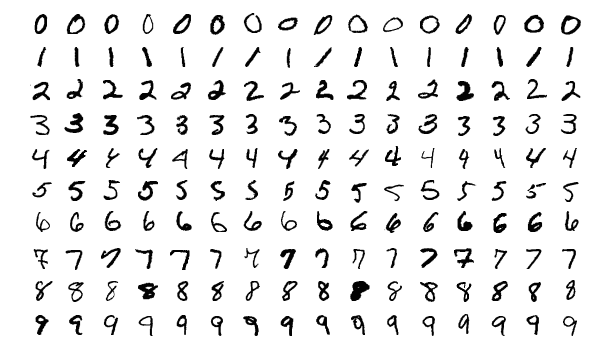
A total number of $5$ independent chains are used for each method on MNIST. The Dropout rate is varied as $p\in[0.1,0.5,0.9]$, and the predictive results are compared with SGHMC and SGLD using the hyper-parameter setting established in the Table 1. The results can be seen in Table 2.

Method	Total Accuracy ($\%$)
SGHMC	$90.94\pm 0.28$
SGLD	$88.06\pm 0.18$
D-SGHMC ($p=0.9$)	$91.66\pm 0.10$
D-SGHMC ($p=0.5$)	$91.72\pm 0.11$
D-SGHMC ($p=0.1$)	$88.26\pm 0.08$

Table 2: Test Accuracy for MNIST data Set. $5$ independent chains.

Compared to other sampling techniques, the results show that D-SGHMC obtains a lower error when the dropout probability is set to $0.5$, which is consistent to the state-of-the-art results in terms of linear classification methods LeCun et al. [1998].

The role of the Dropout probability ($p$) for D-SGHMC is also studied. Figure 2 show accuracy results with the execution of $5$ independent chains. It is possible to establish that for the studied data set a dropout probability between on $0.6$ and $0.8$ generates lower error rates. On the other hand, it can also be seen that probabilities lower than $0.4$ rapidly decreases the variable’s influence on the classification results.

Figure 2: D-SGHMC Sensitivity analysis for $p$ hyper-parameter. $5$ independent chains on MNIST.

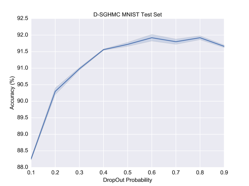
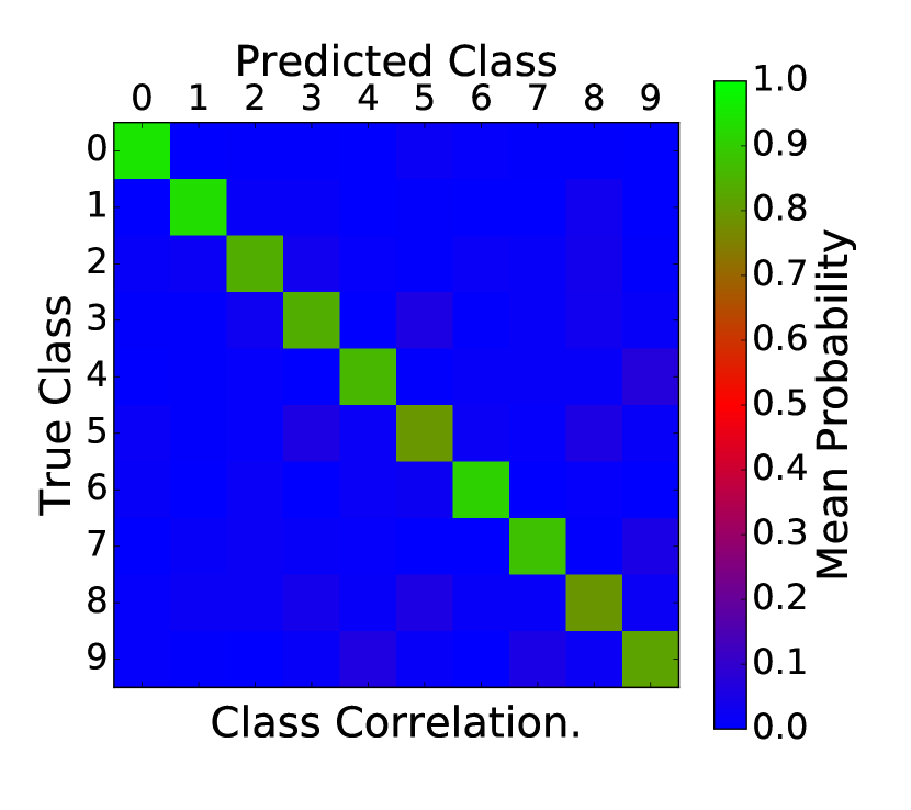
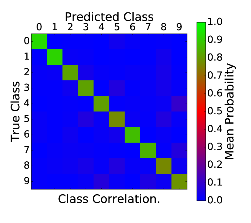
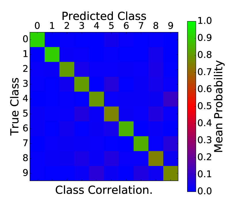
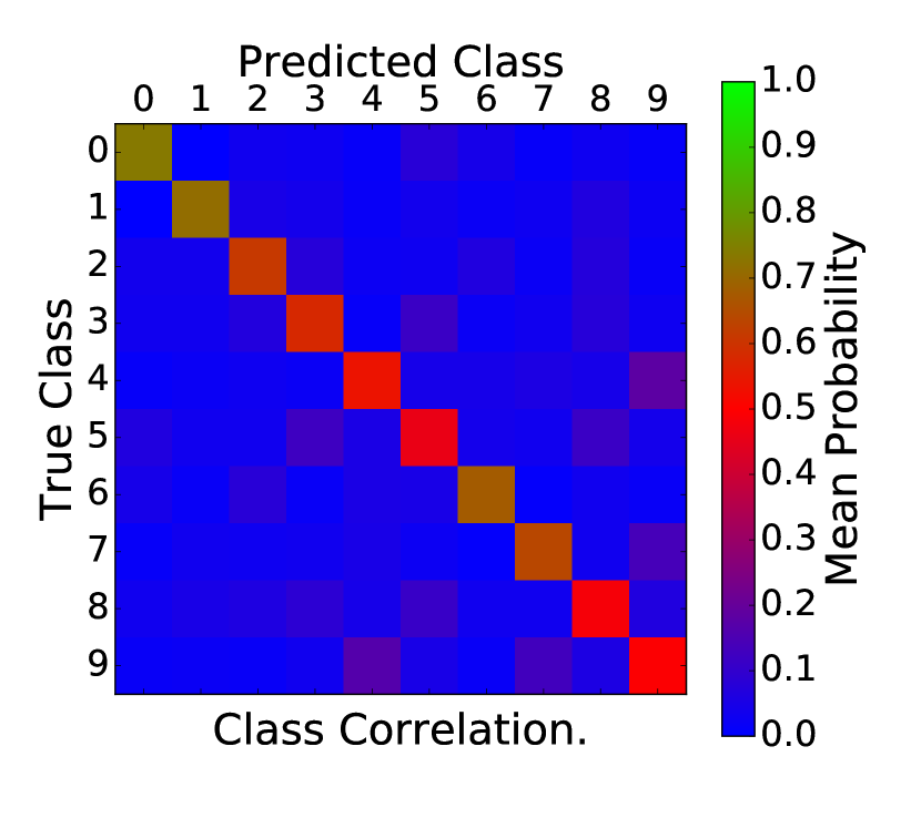
Figure 3 shows the correlation matrix between the true class and the predicted class. Higher class uncertainty is achieved when classifying digits $9$ and $8$ of MNIST, which could be classified as digits $4$ and $5$ respectively.

(a) SGHMC

(b) SGLD

(c) D-SGHMC ($p=0.9$)

(d) D-SGHMC ($p=0.6$)

(e) D-SGHMC ($p=0.5$)

(f) D-SGHMC ($p=0.1$)

Figure 3: Matrix Correlation for error rates on MNIST.

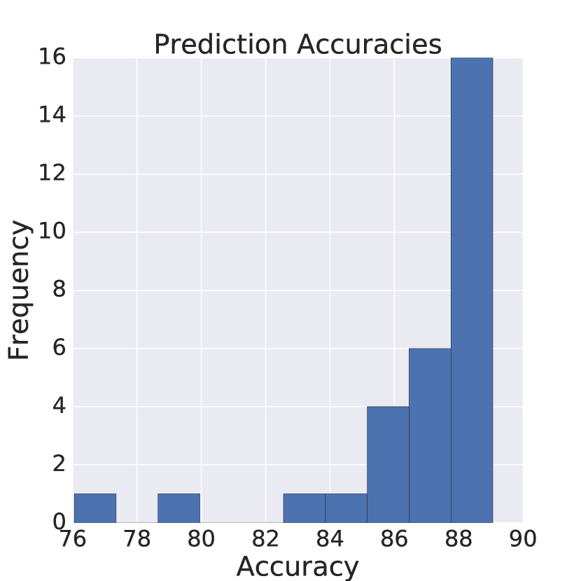
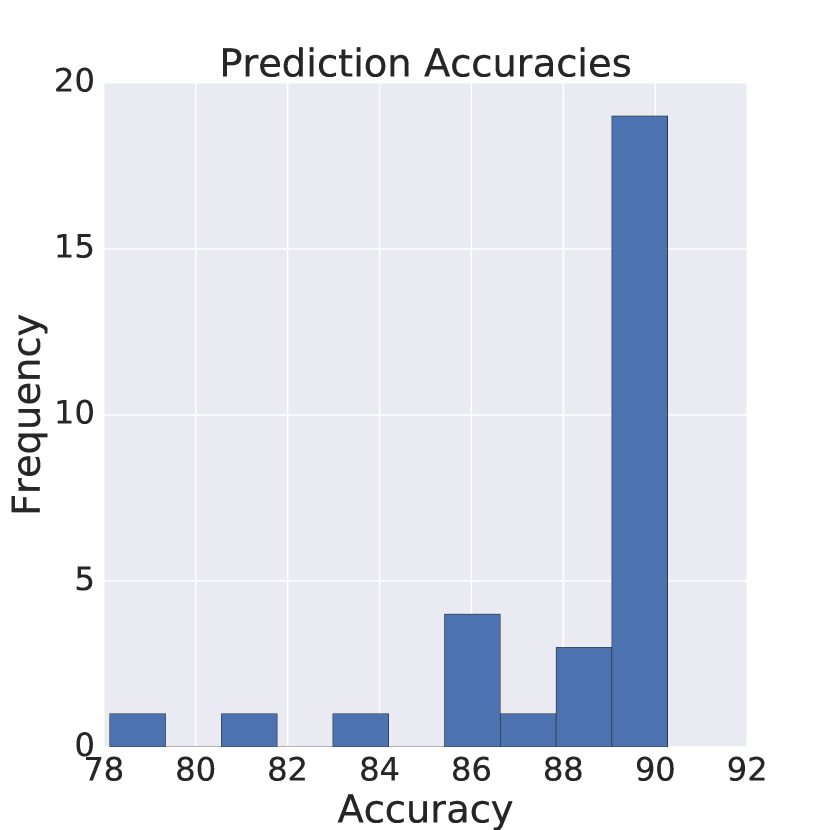
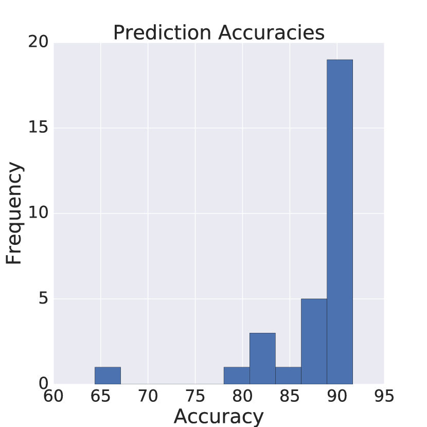
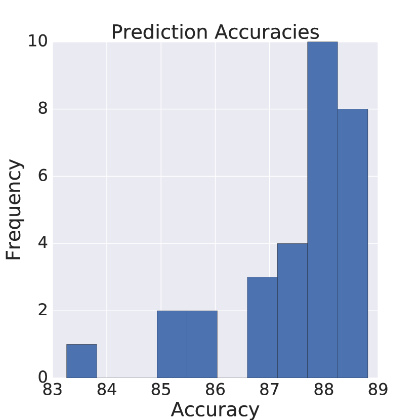
Predictive accuracy is now evaluated by comparing the different methods, where the expected predictive accuracy is computed using a Monte Carlo approximation. D-SGHMC (Fig. 4.a and 4.b) achieves higher predictive accuracy when compared to SGHMC (Fig. 4.c) and SGLD (Fig. 4.d).

(a) D-SGHMC ($p=0.6$)

Predictive accuracy: $92.1\%$

(b) D-SGHMC ($p=0.8$)

Predictive accuracy: $91.9\%$

(c) SGHMC

Predictive accuracy: $90.8\%$

(d) SGLD

Predictive accuracy: $87.9\%$

Figure 4: Histogram of predictive uncertainty.

5.1.1 Confusing classes

One of the biggest challenges of the MNIST data set is to separate highly confusing digits such as ’$4$’ and ’$9$’. This problem has been addressed earlier in feature selection challenges Guyon et al. [2005].

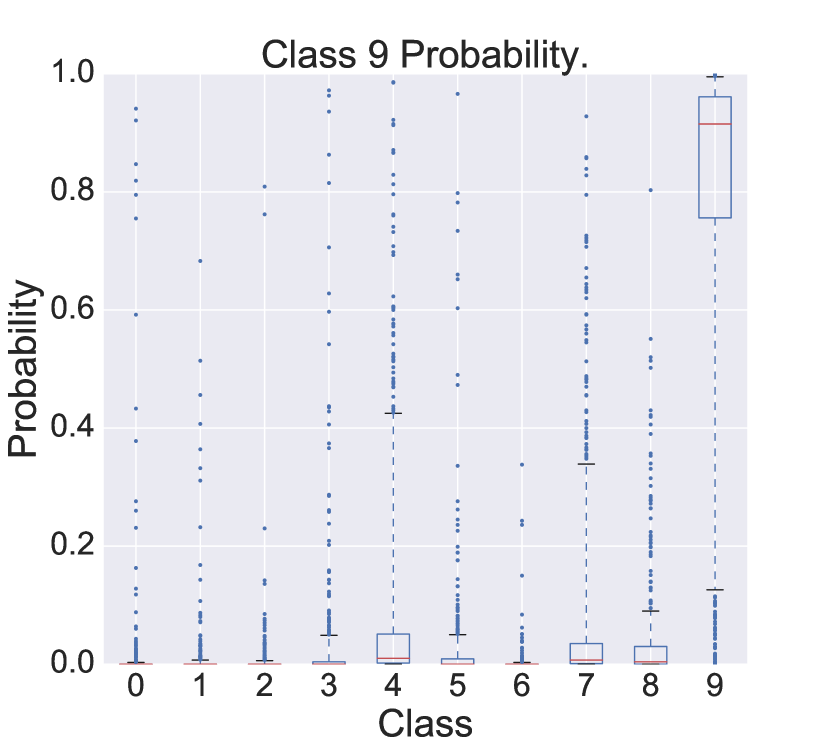
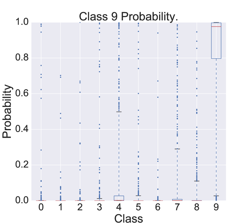
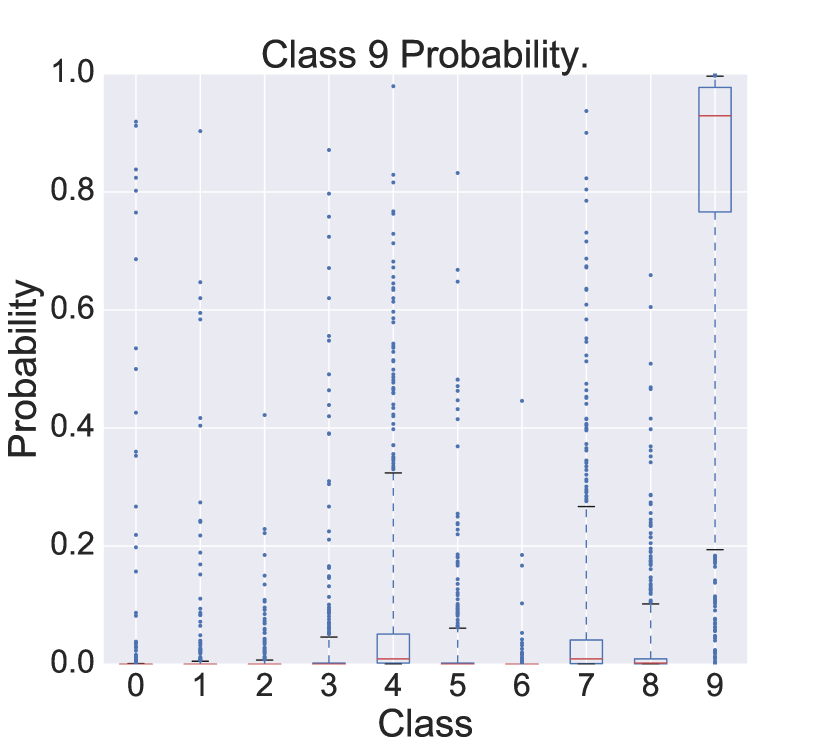
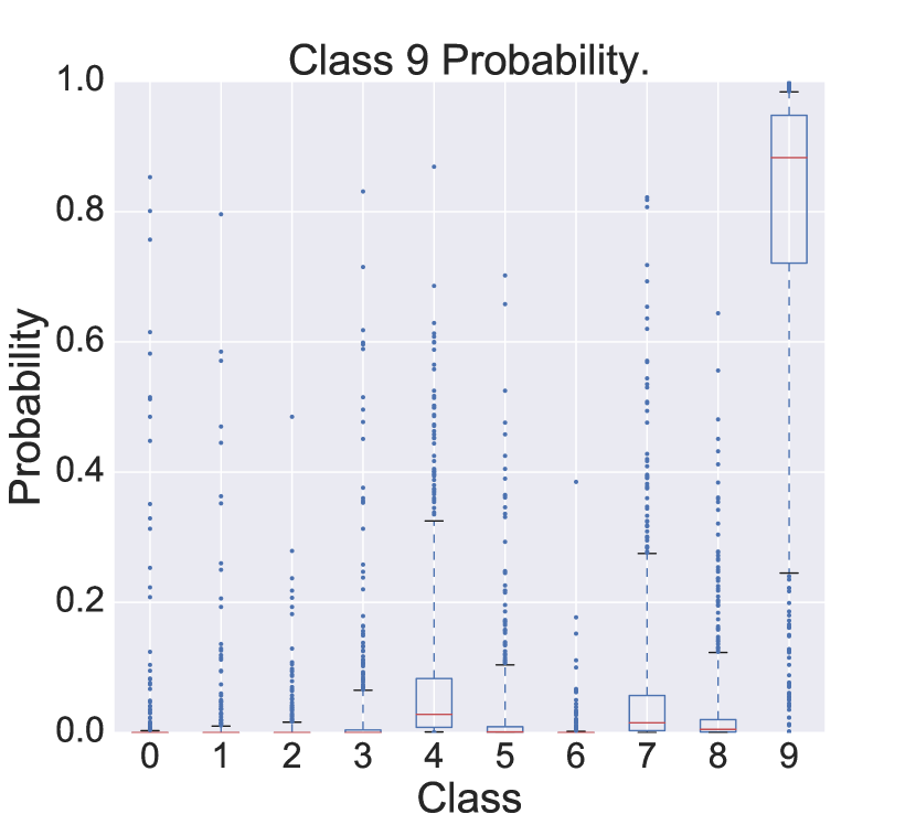
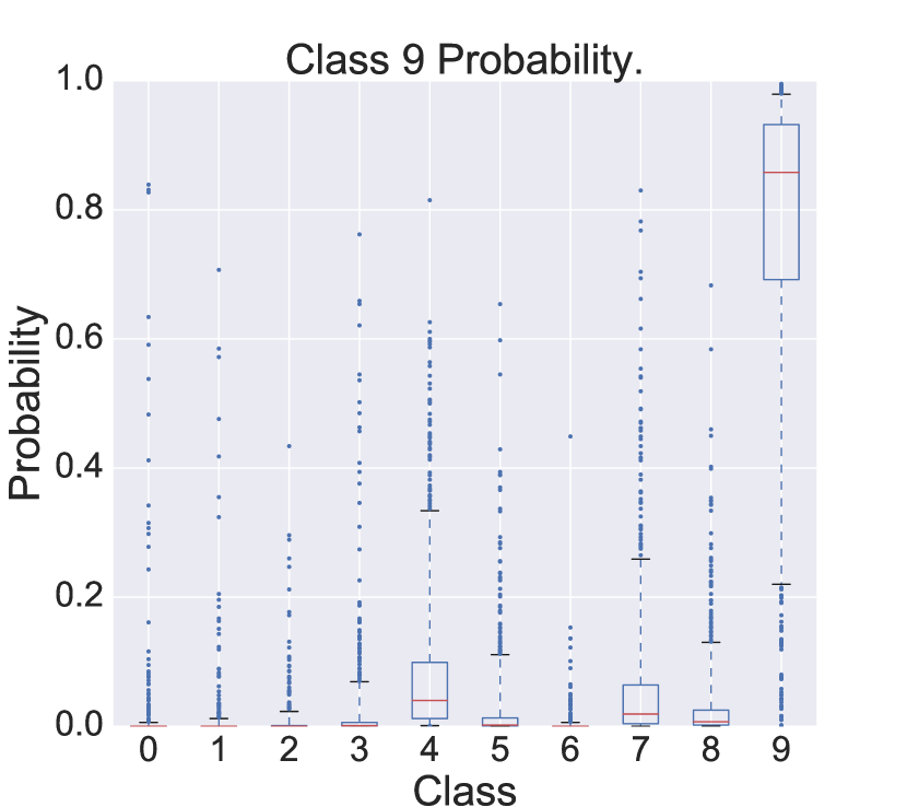
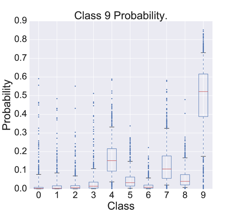
We analyze the behavior between total uncertainty and predictive accuracy for one of these digits in each method. We can observe that there is less over-confidence and at the same time the classification results improve. Figure 5 shows the mean expected probabilities for digit 9 in the test set.

(a) SGHMC

Predictive class accuracy: $87\%$

(b) SGLD

Predictive class accuracy: $84\%$

(c) D-SGHMC ($p=0.9$)

Predictive class accuracy: $90\%$

(d) D-SGHMC ($p=0.6$)

Predictive class accuracy: $92\%$

(e) D-SGHMC ($p=0.5$)

Predictive class accuracy: $91\%$

(f) D-SGHMC ($p=0.1$)

Predictive class accuracy: $86\%$

Figure 5: Box plot of the error rates for class $9$.

As the Dropout rate decreases, the uncertainty around similar classes becomes more visible. However, low Dropout probabilities does not guarantee better classification results or improved uncertainty estimates. As shown in the Figure 5, models generated with low Dropout rates aggressively reduce the number of variables used for prediction.

5.1.2 Confusing Example (digit 9)

In the first example (Fig. 6.a), both state-of-the-art SGHMC (Fig. 6.b) and SGLD methods (Fig. 6.c) maintain a high confidence.

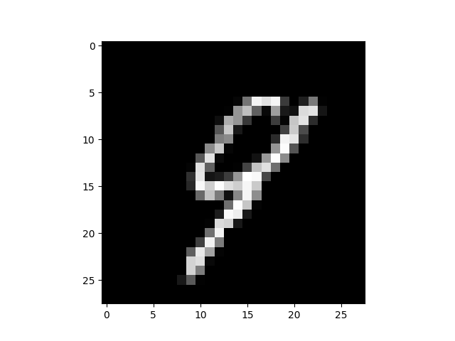
(a) Example digit $9$.

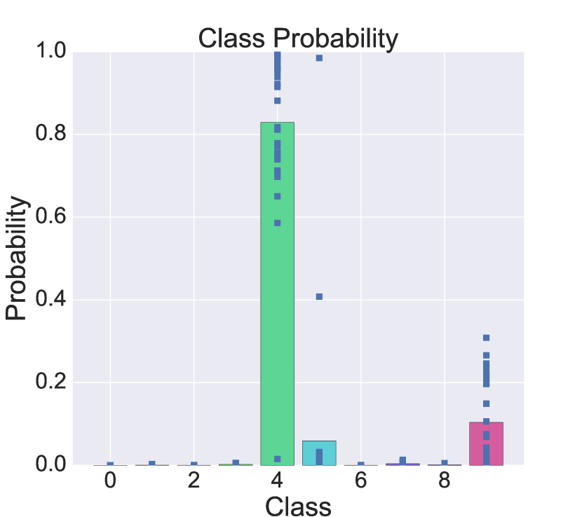
(b) SGHMC

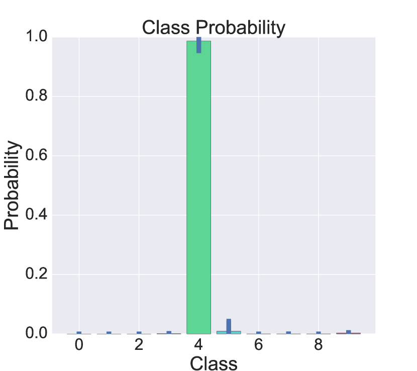
(c) SGLD

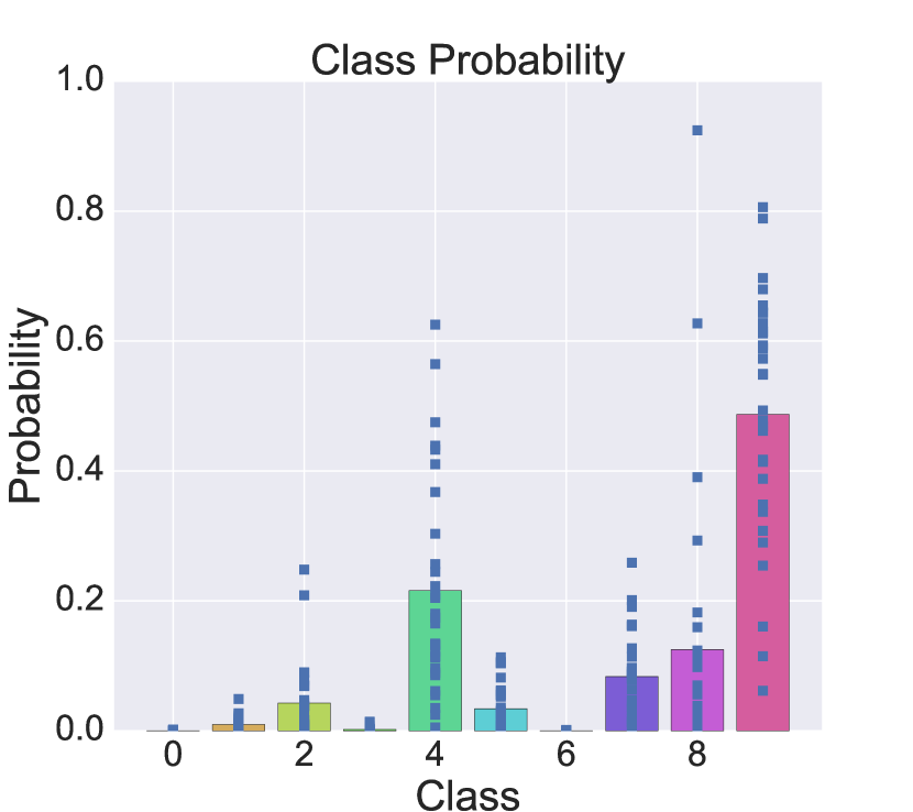
(d) D-SGHMC ($p=0.9$)

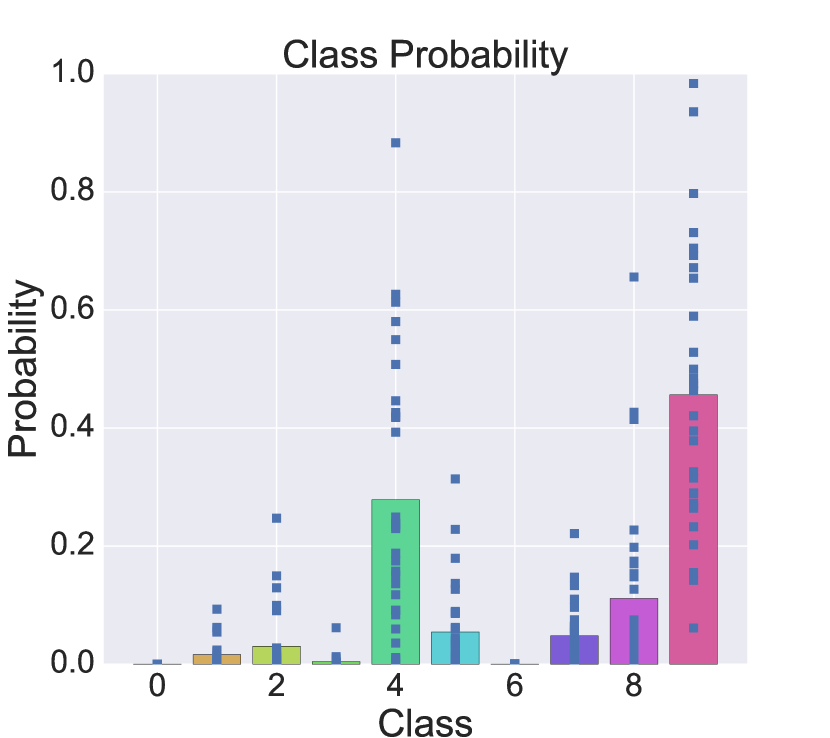
(e) D-SGHMC ($p=0.7$)

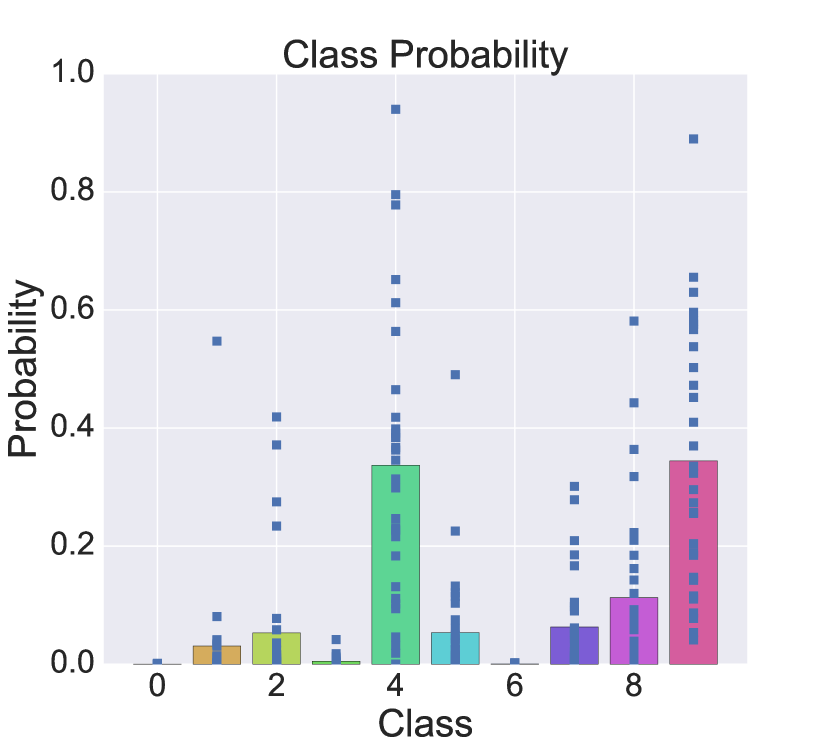
(f) D-SGHMC ($p=0.5$)

Figure 6: Bar plot of error rates for confusing example $9$.

In the example we can see how the proposed method decreases the over-confidence generated by SGHMC and SGLD and allows to classify the example effectively, producing higher uncertainty (Fig. 6.d, 6.e and 6.f).

5.1.3 Confusing Example (digit 8)

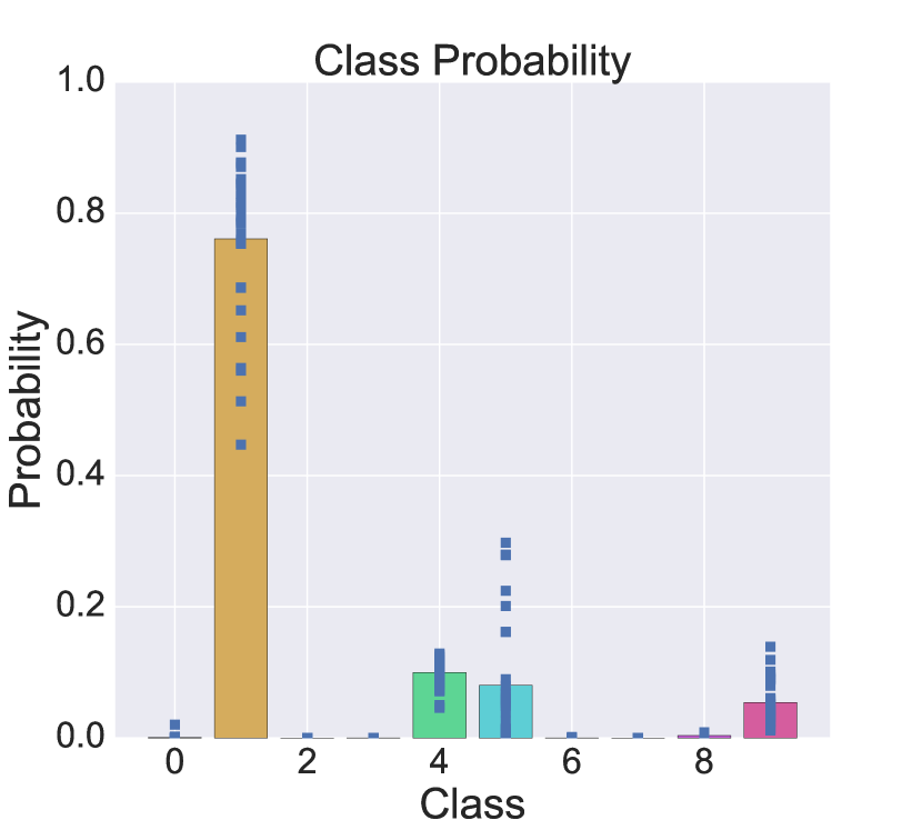
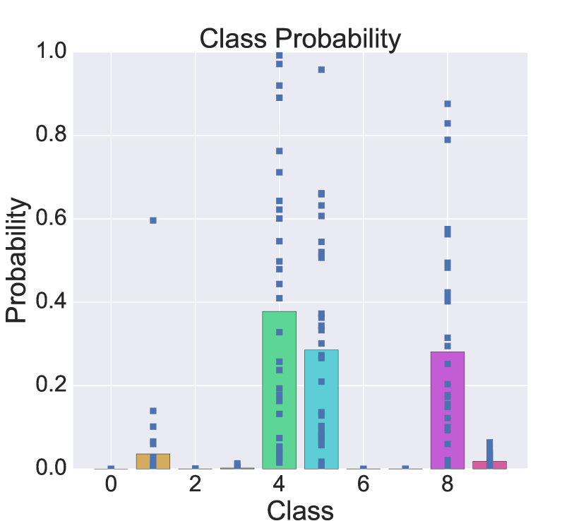
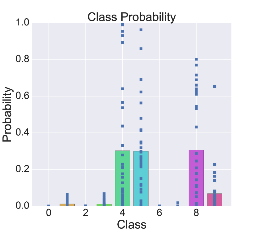
In the second example (Fig. 7.a), we observe that it is similar to the digits ’$4$’, ’$5$’ and even ’$1$’, for thus SGHMC (Fig. 7.b) and SGLD (Fig. 7.c) maintain a high confidence in this digits.

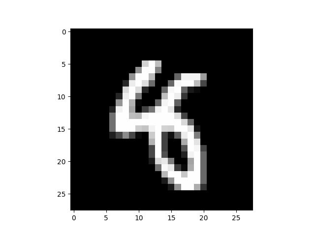
(a) Example digit $8$.

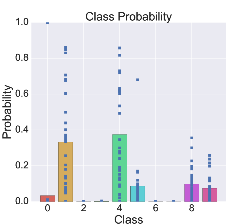
(b) SGHMC

(c) SGLD

(d) D-SGHMC ($p=0.9$)

(e) D-SGHMC ($p=0.7$)

(f) D-SGHMC ($p=0.5$)

Figure 7: Bar plot of error rates for confusing example $8$.

In this example, D-SGHMC does not significantly improve the classification results (Fig. 7.d and 7.f). However, it does improve the uncertainty estimates, generating higher confidence in the true label (Fig. 7.e).

5.2 Age Recognition on ADIENCE

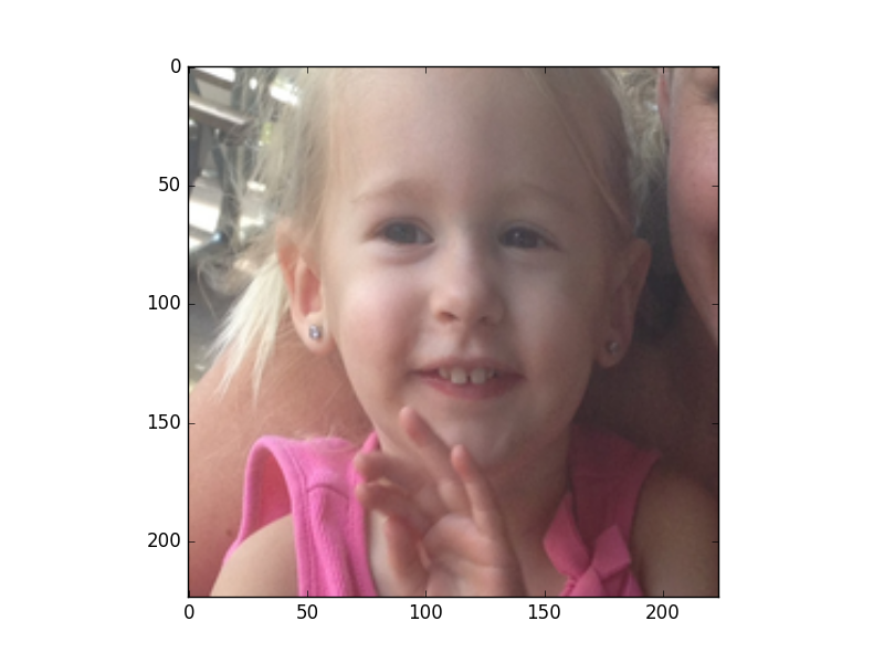
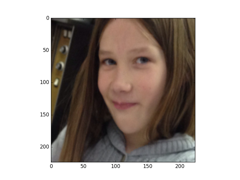
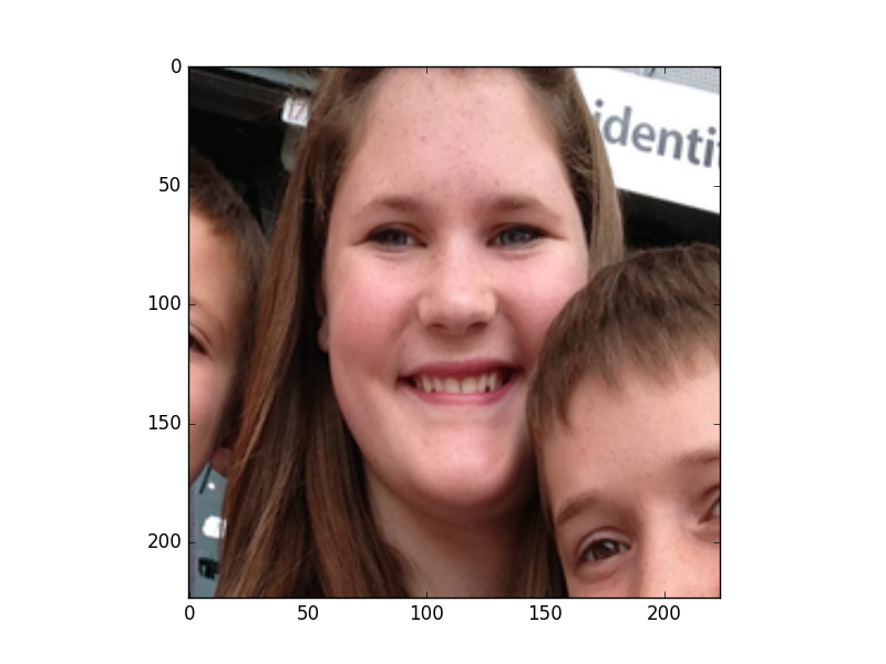
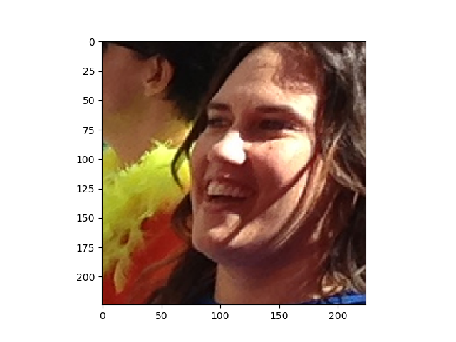
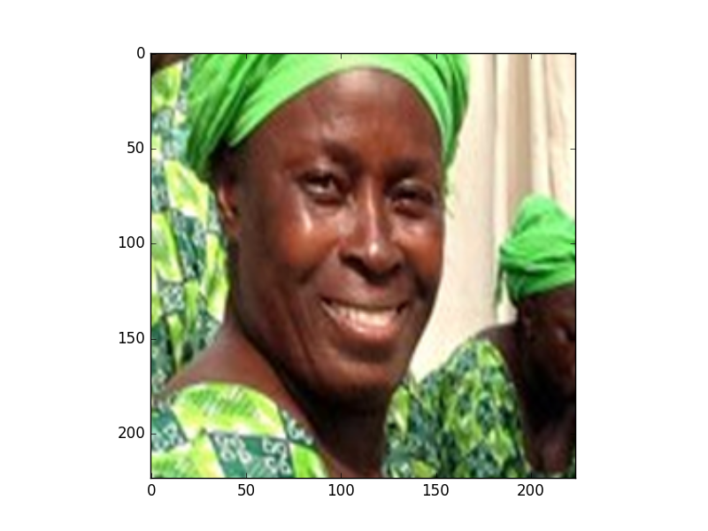
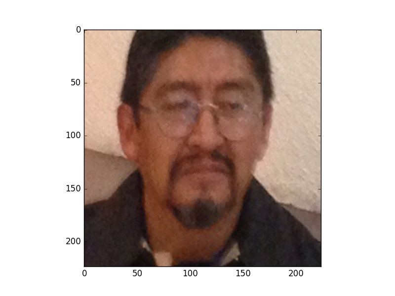
As part of the many challenges of facial recognition systems, age recognition has been recognized as difficult problem Eidinger et al. [2014]. The ADIENCE dataset (see Fig. 8) contains $26.580$ images of $2.284$ different subjects and has been used to study the performance of age and gender recognition systems. After pre-processing and cleaning, the resulting data set is partitioned into $13.000$ training examples and $3.534$ test examples. The final number of samples can be seen in Table 3.

Age	ID Class	Train	Test	Total
[$0-2$]	$0$	$1.201$	$199$	$1.400$
[$4-6$]	$1$	$1.566$	$573$	$2.139$
[$8-13$]	$2$	$1.942$	$343$	$2.285$
[$15-20$]	$3$	$1.385$	$255$	$1.640$
[$25-32$]	$4$	$3.940$	$1.099$	$5.039$
[$38-43$]	$5$	$1.794$	$546$	$2.340$
[$48-53$]	$6$	$579$	$246$	$825$
[$60-$]	$7$	$593$	$273$	$866$
Total	$8$	$13.000$	$3.534$	$16.534$

Table 3: Final examples distribution of the ADIENCE data set.

Figure 8: Examples from ADIENCE database.

Transfer learning from VGG-Face CNN (Convolutional Neural Networks)Parkhi et al. [2015] with AVG pooling is used as a convolutional descriptor. For each example of ADIENCE database, VGG-Face computes a descriptor of $512$ features.

A total number of $5$ independent runs is used for each one of the methods. Using the hyper-parameter setting set in table 1, where state-of-art results are achieved Levi and Hassner [2015]. Comparison with baseline methods can be seen in Table 4.

Method	Total Accuracy ($\%$)
SGHMC	$45.6\pm 1.23$
SGLD	$44.0\pm 1.10$
D-SGHMC($p=0.9)$	$48.2\pm 0.56$
D-SGHMC($p=0.5$)	$51.6\pm 0.51$
D-SGHMC($p=0.1$)	$48.3\pm 0.88$

Table 4: Test accuracy for ADIENCE data Set.

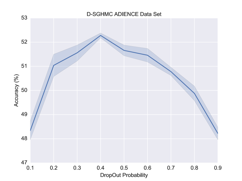
The role of the Dropout rate $p$ on the performance is analyzed. As shown in Figure 9, best results are obtained with values between $0.3$ and $0.5$.

Figure 9: Sensitivity analysis for D-SGHMC with Dropout rate $p$.

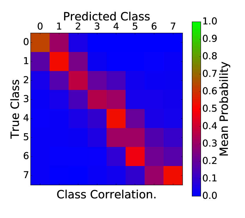
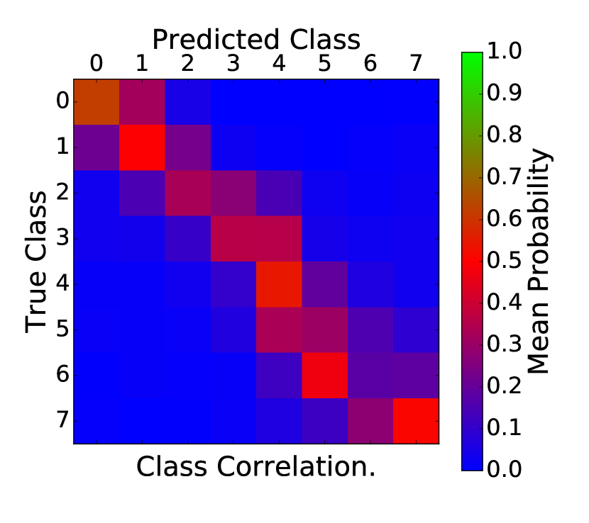
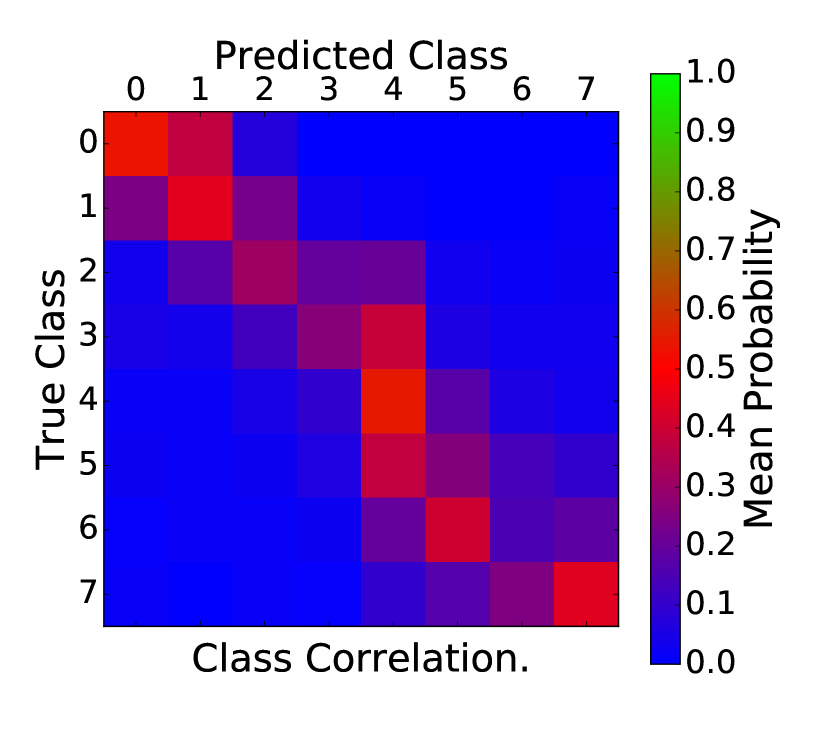
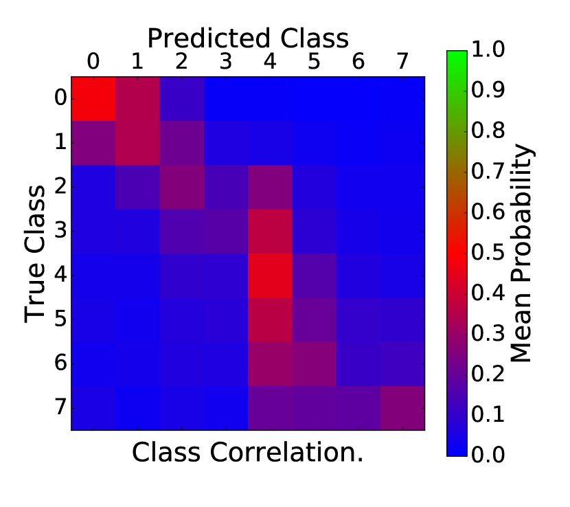
In ADIENCE, uncertainty is increased for neighboring classes. This can be seen in Figure 10, which shows the true and the predicted labels.

(a) SGHMC

(b) SGLD

(c) D-SGHMC ($p=0.9$)

(d) D-SGHMC ($p=0.5$)

(e) D-SGHMC ($p=0.4$)

(f) D-SGHMC ($p=0.1$)

Figure 10: Matrix Correlation plot of probabilities for all classes. $5$ independent chains on ADIENCE.

5.2.1 Accuracy

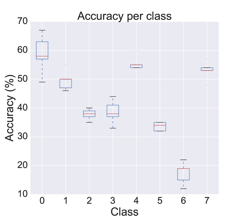
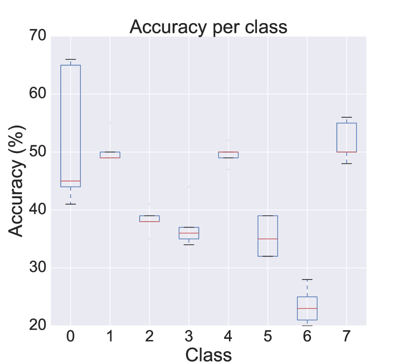
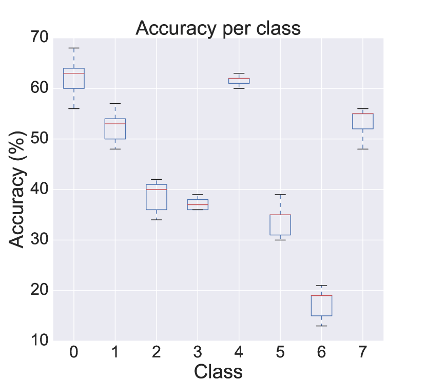
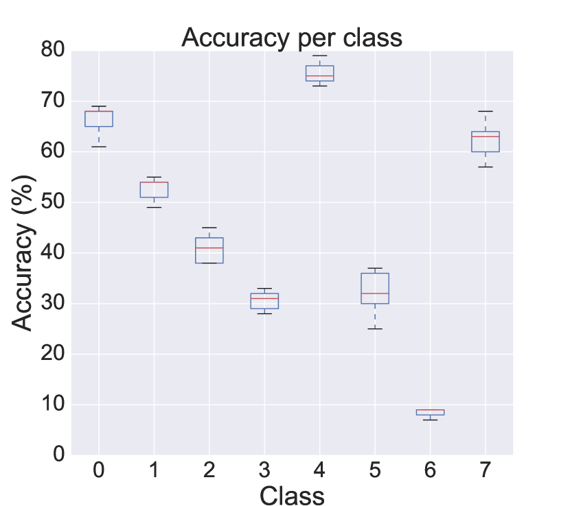
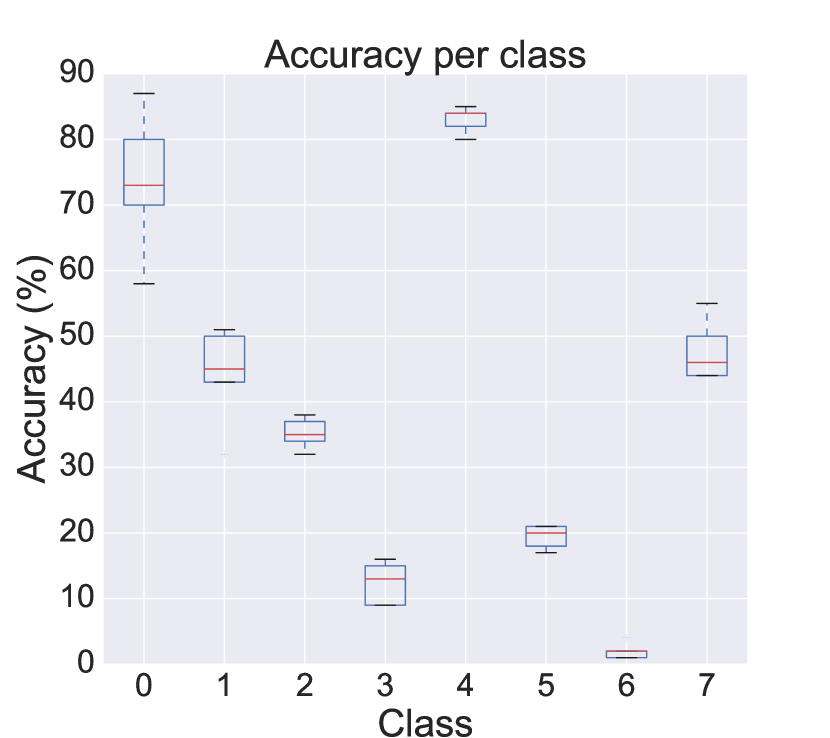
Class imbalance plays an important role in the final classification results for the age recognition problem in ADIENCE. D-SGHMC (see Figure 11.d) improves results in most of classes, sacrificing to a lesser extent the accuracy for classes with less number of examples.

(a) SGHMC

(b) SGLD

(c) D-SGHMC ($p=0.9$)

(d) D-SGHMC ($p=0.5$)

(e) D-SGHMC ($p=0.4$)

(f) D-SGHMC ($p=0.1$)

Figure 11: Box plot of accuracies for all classes on ADIENCE.

As the Dropout rate decreases, the imbalance problem becomes more evident and the accuracy results are also dropped (see Figure 9 ).

5.2.2 Predictive Uncertainty for the Adience Dataset

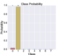
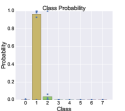
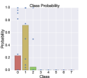
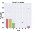
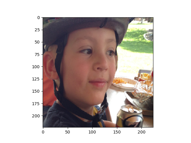
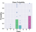
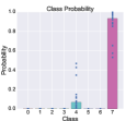
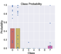
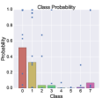
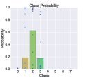
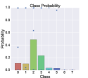
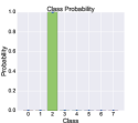
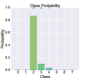
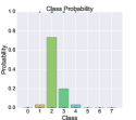
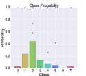
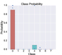
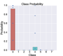
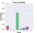
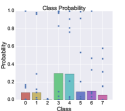
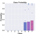
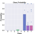
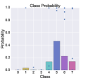
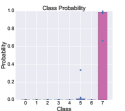
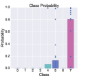
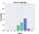
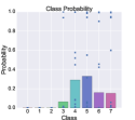
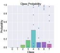
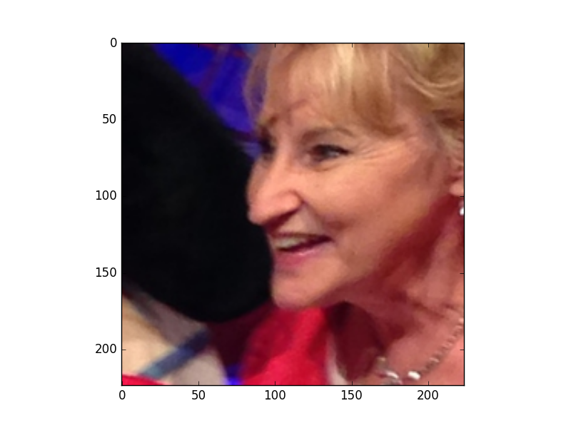
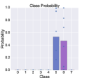
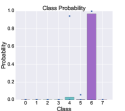
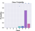
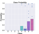
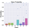
In the ADIENCE data set there are many confusing examples which are usually neighboring classes. One example for each class is randomly sampled and the predictive distributions for each model are evaluated. These results are shown in Figure 12. In general, SGHMC and SGLD produce over-confident probabilities,assigning high values to incorrect labels. In contrast, D-SGHMC reduces that confidence, increasing uncertainty in the class predictions.

In particular, high confidence estimates for both SGHMC and SGLD on one example of class $4$ can be seen in Figure 12. On the other hand, the proposed method allows to improve the uncertainty estimates between the neighboring classes, which significantly improves the classification results.

This situation is also replicated on one example of class $7$, where SGHMC and SGLD achieves over-confident misclassification (class $1$). The proposed method allows to alleviate the misclassification error and return uncertainty estimates for neighboring classes. The predictive distribution improves the classification results and provides the improved uncertainty estimates.

Class

SGHMC

SGLD

D-SGHMC ($p=0.9$)

D-SGHMC ($p=0.5$)

D-SGHMC ($p=0.1$)

Class 0

Class 1

Class 2]

Class 3

Class 4

Class 5

Class 6

Class 7

Figure 12: Predictive distribution for randomly selected samples from the ADIENCE dataset.

6 Conclusion

In many decision-making systems, the estimated uncertainty plays a crucial role in the final classification. Over-confident estimates can arise from noisy examples or when leading with classes that were not part of the training data set. The fundamental objective of achieving improved uncertainty estimates is to encourage decision-makers to question their decisions. In this way, compared to other state-of-the-art MCMC methods for large scale and high dimensional classification problems, the methodology presented in this paper improves the uncertainty estimated.

The proposed method is based on HMC and Dropout regularization. The experiments demonstrated that the method is capable of generating an approximation to the posterior distribution. In addition, the resulting predictive distributions also alleviate the misclassification error in difficult examples. However, it has not yet been proven that generated stochastic dynamics preserve the volume in its entirety. Future work will perform comparisons with other state-of-the-art variational methods. Moreover, the relationship between the proposed approach to approximate Bayesian model averaging can be also another line of research.

Compliance with Ethical Standards

Funding This work was supported by two CONICYT grants. Project CONICYT/FONDECYT Robust Multi-Target Tracking using Discrete Visual Features code 11140598. Project CONICYT/PFCHA Beca Magister Nacional 2017 code 22170718. Ethical approval This article does not contain any studies with human participants or animals performed by any of the authors.

References

- Afshar and Domke [2015] H. M. Afshar and J. Domke. Reflection, refraction, and Hamiltonian Monte Carlo. In Advances in Neural Information Processing Systems, pages 3007–3015, 2015.
- Baldi and Sadowski [2014] P. Baldi and P. Sadowski. The dropout learning algorithm. Artificial intelligence, 210:78–122, 2014.
- Baldi and Sadowski [2013] P. Baldi and P. J. Sadowski. Understanding dropout. In Advances in neural information processing systems, pages 2814–2822, 2013.
- Bardenet et al. [2014] R. Bardenet, A. Doucet, and C. Holmes. Towards scaling up Markov chain Monte Carlo: an adaptive subsampling approach. In International Conference on Machine Learning, pages 405–413, 2014.
- Beskos et al. [2013] A. Beskos, N. Pillai, G. Roberts, J.-M. Sanz-Serna, A. Stuart, et al. Optimal tuning of the hybrid monte carlo algorithm. Bernoulli, 19(5A):1501–1534, 2013.
- Bishop [2007] C. M. Bishop. Pattern recognition and machine learning (information science and statistics), 1st edn. 2006. corr. 2nd printing edn. Springer, New York, 2007.
- Carpenter et al. [2017] B. Carpenter, A. Gelman, M. D. Hoffman, D. Lee, B. Goodrich, M. Betancourt, M. Brubaker, J. Guo, P. Li, and A. Riddell. Stan: A probabilistic programming language. Journal of Statistical Software, 76(1), 2017.
- Chaari et al. [2016] L. Chaari, J.-Y. Tourneret, C. Chaux, and H. Batatia. A hamiltonian monte carlo method for non-smooth energy sampling. IEEE Transactions on Signal Processing, 64(21):5585–5594, 2016.
- Chen et al. [2014] T. Chen, E. Fox, and C. Guestrin. Stochastic gradient hamiltonian monte carlo. In International Conference on Machine Learning, pages 1683–1691, 2014.
- Eidinger et al. [2014] E. Eidinger, R. Enbar, and T. Hassner. Age and gender estimation of unfiltered faces. IEEE Transactions on Information Forensics and Security, 9(12):2170–2179, 2014.
- Gal and Ghahramani [2016] Y. Gal and Z. Ghahramani. Dropout as a bayesian approximation: Representing model uncertainty in deep learning. In international conference on machine learning, pages 1050–1059, 2016.
- Gelman et al. [2014] A. Gelman, J. B. Carlin, H. S. Stern, D. B. Dunson, A. Vehtari, and D. B. Rubin. Bayesian data analysis, volume 2. CRC press Boca Raton, FL, 2014.
- Girolami and Calderhead [2011] M. Girolami and B. Calderhead. Riemann manifold langevin and hamiltonian monte carlo methods. Journal of the Royal Statistical Society: Series B (Statistical Methodology), 73(2):123–214, 2011.
- Griewank and Walther [2008] A. Griewank and A. Walther. Evaluating Derivatives: Principles and Techniques of Algorithmic Differentiation. Society for Industrial and Applied Mathematics, Philadelphia, PA, USA, second edition, 2008. ISBN 0898716594, 9780898716597.
- Guyon et al. [2005] I. Guyon, S. Gunn, A. Ben-Hur, and G. Dror. Result analysis of the nips 2003 feature selection challenge. In Advances in neural information processing systems, pages 545–552, 2005.
- Hoffman [2017] M. D. Hoffman. Learning deep latent gaussian models with markov chain monte carlo. In International Conference on Machine Learning, pages 1510–1519, 2017.
- Hoffman and Gelman [2014] M. D. Hoffman and A. Gelman. The no-u-turn sampler: adaptively setting path lengths in hamiltonian monte carlo. Journal of Machine Learning Research, 15(1):1593–1623, 2014.
- Kingma et al. [2015] D. P. Kingma, T. Salimans, and M. Welling. Variational dropout and the local reparameterization trick. In C. Cortes, N. D. Lawrence, D. D. Lee, M. Sugiyama, and R. Garnett, editors, Advances in Neural Information Processing Systems 28, pages 2575–2583. Curran Associates, Inc., 2015.
- LeCun et al. [1998] Y. LeCun, L. Bottou, Y. Bengio, and P. Haffner. Gradient-based learning applied to document recognition. Proceedings of the IEEE, 86(11):2278–2324, 1998.
- Leibig et al. [2017] C. Leibig, V. Allken, M. S. Ayhan, P. Berens, and S. Wahl. Leveraging uncertainty information from deep neural networks for disease detection. Scientific reports, 7(1):17816, 2017.
- Levi and Hassner [2015] G. Levi and T. Hassner. Age and gender classification using convolutional neural networks. In Proceedings of the IEEE Conference on Computer Vision and Pattern Recognition Workshops, pages 34–42, 2015.
- Li and Hoiem [2018] Z. Li and D. Hoiem. Learning without forgetting. IEEE Transactions on Pattern Analysis and Machine Intelligence, pages 1–1, 2018. ISSN 0162-8828. doi: 10.1109/TPAMI.2017.2773081.
- Miceli Barone et al. [2017] A. V. Miceli Barone, B. Haddow, U. Germann, and R. Sennrich. Regularization techniques for fine-tuning in neural machine translation. In Proceedings of the 2017 Conference on Empirical Methods in Natural Language Processing, pages 1489–1494, Copenhagen, Denmark, September 2017. Association for Computational Linguistics.
- Neal [2012] R. M. Neal. Bayesian learning for neural networks, volume 118. Springer Science & Business Media, 2012.
- Neal et al. [2011] R. M. Neal et al. MCMC using hamiltonian dynamics. Handbook of Markov Chain Monte Carlo, 2(11), 2011.
- Nishimura et al. [2017] A. Nishimura, D. Dunson, and J. Lu. Discontinuous hamiltonian monte carlo for models with discrete parameters and discontinuous likelihoods. arXiv preprint arXiv:1705.08510, 2017.
- Pakman and Paninski [2013] A. Pakman and L. Paninski. Auxiliary-variable exact hamiltonian monte carlo samplers for binary distributions. In Advances in neural information processing systems, pages 2490–2498, 2013.
- Parkhi et al. [2015] O. M. Parkhi, A. Vedaldi, and A. Zisserman. Deep face recognition. In British Machine Vision Conference, 2015.
- Pearl [1988] J. Pearl. Probabilistic Reasoning in Intelligent Systems: Networks of Plausible Inference. Morgan Kaufmann Publishers Inc., San Francisco, CA, USA, 1988. ISBN 0-934613-73-7.
- Pereyra [2016] M. Pereyra. Proximal markov chain monte carlo algorithms. Statistics and Computing, 26(4):745–760, 2016.
- Prince [2012] S. J. Prince. Computer vision: models, learning, and inference. Cambridge University Press, 2012.
- Roberts and Rosenthal [1998] G. O. Roberts and J. S. Rosenthal. Optimal scaling of discrete approximations to langevin diffusions. Journal of the Royal Statistical Society: Series B (Statistical Methodology), 60(1):255–268, 1998.
- Roberts and Stramer [2002] G. O. Roberts and O. Stramer. Langevin diffusions and metropolis-hastings algorithms. Methodology and computing in applied probability, 4(4):337–357, 2002.
- Srivastava et al. [2014] N. Srivastava, G. Hinton, A. Krizhevsky, I. Sutskever, and R. Salakhutdinov. Dropout: A simple way to prevent neural networks from overfitting. The Journal of Machine Learning Research, 15(1):1929–1958, 2014.
- Tran et al. [2017] D. Tran, M. D. Hoffman, R. A. Saurous, E. Brevdo, K. Murphy, and D. M. Blei. Deep probabilistic programming. In International Conference on Learning Representations, 2017.
- Wan et al. [2013] L. Wan, M. Zeiler, S. Zhang, Y. L. Cun, and R. Fergus. Regularization of neural networks using dropconnect. In Proceedings of the 30th international conference on machine learning (ICML-13), pages 1058–1066, 2013.
- Wang et al. [2013] Z. Wang, S. Mohamed, and N. Freitas. Adaptive hamiltonian and riemann manifold monte carlo. In International Conference on Machine Learning, pages 1462–1470, 2013.
- Warde-Farley et al. [2013] D. Warde-Farley, I. J. Goodfellow, A. Courville, and Y. Bengio. An empirical analysis of dropout in piecewise linear networks. arXiv preprint arXiv:1312.6197, 2013.
- Welling and Teh [2011] M. Welling and Y. W. Teh. Bayesian learning via stochastic gradient langevin dynamics. In Proceedings of the 28th International Conference on Machine Learning (ICML-11), pages 681–688, 2011.