Optimal switching sequence for switched linear systems

Abstract

We study the following optimization problem over a dynamical system that consists of several linear subsystems: Given a finite set of $n\times n$ matrices and an $n$-dimensional vector, find a sequence of $K$ matrices, each chosen from the given set of matrices, to maximize a convex function over the product of the $K$ matrices and the given vector. This simple problem has many applications in operations research and control, yet a moderate-sized instance is challenging to solve to optimality for state-of-the-art optimization software. We propose a simple exact algorithm for this problem. Our algorithm runs in polynomial time when the given set of matrices has the oligo-vertex property, a concept we introduce in this paper for a finite set of matrices. We derive several sufficient conditions for a set of matrices to have the oligo-vertex property. Numerical results demonstrate the clear advantage of our algorithm in solving large-sized instances of the problem over one state-of-the-art global optimization solver. We also propose several open questions on the oligo-vertex property and discuss its potential connection with the finiteness property of a set of matrices, which may be of independent interest.

1 Introduction

Many real-world systems exhibit significantly different dynamics under various modes or conditions, for example a manual transmission car operating at different gears, a chemical reactor under different temperatures and flow rates of reactants, and a group of cancer cells responding to different drugs. Such phenomena can be modeled under a unified framework of switched systems. A switched system is a dynamical system that consists of several subsystems and a rule that specifies the switching among the subsystems. Finding a switching rule to optimize the dynamics of a switched system under certain criteria has found numerous applications in power system operations, chemical process control, air traffic management, and medical treatment design [39, 26, 25, 16]. In this paper, we study the following discrete-time switched linear system:

$$x(k+1)=T_{k}x(k),\qquad T_{k}\in\Sigma,\;k=0,1,\ldots,$$ (1)

where $x(k)$ is an $n$-dimensional real vector that captures the system state at period $k$, the set $\Sigma$ contains $m$ real matrices in $\mathbb{R}^{n\times n}$, each of which describes the dynamics of a linear subsystem, and the initial vector $x(0)$ is a given $n$-dimensional real vector $a$. Such a system with switching only at fixed time instants appear in many practical applications, and is also employed to approximate the more complex dynamics of a continuous-time hybrid system with switching times defined over the real line [39, 25].

We are interested in the following optimization problem $(\mathrm{P})$ related to the system in (1):

Given a switched linear system described in (1), a positive integer $K$, and a convex function $f:\mathbb{R}^{n}\rightarrow\mathbb{R}$, find a sequence of $K$ matrices $T_{0},T_{1},\ldots,T_{K-1}\in\Sigma$ to maximize $f(x(K))$.

One type of such convex functions are the $\ell_{p}$ norms.

Example 1.

Consider a switched linear system consisting of two subsystems with system matrices $A=\begin{bmatrix}1&1\\ 1&0\end{bmatrix}$ and $B=\begin{bmatrix}1&1\\ 0&1\end{bmatrix}$, an initial vector $a=(2,1)^{\top}$, and $K=8$. Figure 1 illustrates the trajectory of $x(k)$ under three different switching sequences, with the final state $x(8)$ being $(53,23)^{\top}$, $(58,41)^{\top}$, and $(71,41)^{\top}$, respectively.

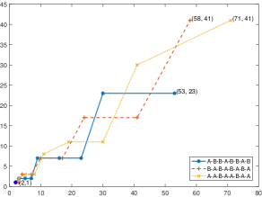
Figure 1: The trajectory of $x(k)$ under three matrix sequences

We give three examples below to illustrate the applications of Problem $(\mathrm{P})$ and its connection to other problems in control and optimization.

The first example is on design of treatment plans. Antibiotic resistance renders diseases that were once easily treatable dangerous infections, and has become one of the most pressing public health problems around the world. Several groups of researchers studied how to design sequential antibiotic treatment plans to restore susceptibility after bacteria develop resistance [29, 31]. They model the percentages of $n$ genotypes of an enzyme produced by bacteria in a population after $k$ periods of treatment with the vector $x(k)$, and model the mutation rates among $n$ genotypes under each antibiotic with a probability transition matrix. The goal is to design a sequence of antibiotics to maximize the percentage of the wild type at the end of the treatment, which is sensitive to all antibiotics. The treatment design problem is equivalent to solve $(\mathrm{P})$ with $a=e_{1}$, a unit vector with the first component being 1 which denotes $100\%$ wild type in the beginning, and $f(x(K))=-e_{1}^{\top}x(K)$. In the same vein, $(\mathrm{P})$ can model the sequential therapy design problem for many other diseases when $x(k)$ describes the related biometrics of a patient at period $k$ and each matrix models the evolution of patient biometrics under a particular treatment [16].

The second example is the matrix mortality problem in control [6, 7]. Given a positive integer $k$, a set of matrices is said to be $k$-mortal if the zero matrix can be expressed as a product of $k$ matrices in the set (duplication allowed). A set of matrices is said to be mortal if it is $k$-mortal for some finite $k$. The matrix mortality problem captures the stability of switched linear systems under certain switching rules. It can be shown that a finite set of $n\times n$ non-negative matrices is $k$-mortal if and only if the optimal objective value of $(\mathrm{P})$ is 0 with $a=\mathbf{1}$, $K=k$, and $f(x(K))=-\mathbf{1}^{\top}x(K)$, where $\mathbf{1}$ is an $n$-dimensional vector with each component being 1.

The third example concerns the joint spectral radius of a set of matrices, an important quantity which has found many applications in wavelet functions, constrained coding, and network security management, etc [18]. The joint spectral radius of a finite set $\Sigma$ of matrices is defined as $\rho(\Sigma)=\limsup_{k\rightarrow\infty}\hat{\rho}_{k}(\Sigma,\|\cdot\|)$ [36], where

$$\hat{\rho}_{k}(\Sigma,\|\cdot\|)=\max\{\|T_{k-1}T_{k-2}\ldots T_{0}\|^{1/k}\mid T_{j}\in\Sigma,j=0,\ldots,k-1\}$$ (2)

and $\|\cdot\|$ is some matrix norm. If we select the matrix norm in (2) to be induced by the $\ell_{p}$ norm of a vector, then

$$(\hat{\rho}_{k}(\Sigma,\|\cdot\|))^{k}=\sup_{\|a\|_{p}=1}\max\{\|x(K)\|_{p}\mid\eqref{eq_switched_system}\}.$$ (3)

Observe that the inner maximization problem of the right-hand side of (3) is a special case of $(\mathrm{P})$ with the convex function $f(x)=\|x\|_{p}$. In general, let $v^{*}$ be the optimal objective value of $(\mathrm{P})$ with $f(x)=\|x\|$ for some norm $\|\cdot\|$ and an initial vector $a$. Then $(v^{*})^{1/k}$ provides a lower bound of the quantity $\hat{\rho}_{k}(\Sigma,\|\cdot\|)$.

A simple way to solve $(\mathrm{P})$ is to enumerate all possible matrix sequences, but such an approach quickly becomes impractical as $m$ and $K$ increase. Even for $m=5$ and $K=30$, we need to enumerate $5^{30}$ solutions, a formidable task for the current fastest computer. Another general approach to solve $(\mathrm{P})$ is to formulate it as a mixed-integer nonlinear optimization problem, which can be solved by global optimization solvers, but the problem size that can be handled by state-of-the-art commercial solvers is also limited. In addition, the time complexity of the tree-based search algorithms employed by these global solvers is difficult to analyze in general. In many applications, problem $(\mathrm{P})$ has to be solved repeatedly with different parameters, so it is of vital importance to have a fast algorithm for $(\mathrm{P})$.

We now present our results. We develop a simple dynamic programming algorithm to solve $(\mathrm{P})$ exactly, which means that an optimal matrix sequence is guaranteed at the termination of the algorithm. Our algorithm is much faster than the state-of-the-art global optimization solver Baron in solving the same instance of $(\mathrm{P})$. Another advantage of our algorithm is that it does not require any additional property of the function $f$ such as smoothness or strong convexity. The main idea of our algorithm is to find out the extreme points of a polytope by iteratively constructing the convex hull of linear transformations of another polytope’s extreme points. As pointed out by one referee, this idea has been used before to construct a special polytope needed to compute the joint spectral radius of a finite set of matrices [13].

Furthermore, we introduce a new concept for a finite set of matrices to analyze the time complexity of our algorithm. In particular, we assume that all input data are integers and the value of the convex function $f$ can be queried through an oracle in constant time; we adopt the random-access machine [32] as the model of computation, in which each basic operation (addition, comparison, multiplication, etc.) is assume to take the same amount of time and the time complexity of an algorithm is the number of steps/operations required to execute the algorithm. We define the following notations that are useful for presenting the time-complexity results. Given a finite set $\Sigma$ of $n\times n$ real matrices and a vector $a\in\mathbb{R}^{n}$, let

$$P_{k}(\Sigma,a):=\mathrm{conv}(\{x(k)\mid x(k)=T_{k-1}\cdots T_{0}a,T_{j}\in\Sigma,j=0,\ldots,k-1\})$$

be the convex hull of all possible values of $x(k)$ in (1) for each integer $k\geq 0$. Let $N_{k}(\Sigma,a)$ be the number of extreme points of $P_{k}(\Sigma,a)$ and

$$N_{k}(\Sigma)=\sup_{a\in\mathbb{R}^{n}}\{N_{k}(\Sigma,a)\}.$$

We introduce the following concept for a set of matrices.

Definition 1.

A set of matrices $\Sigma$ is said to have the oligo-vertex property if there exists $\alpha>0$, positive integer $k_{0}$, and positive constant $d$ such that $N_{k}(\Sigma)\leq\alpha k^{d}$ for any $k\geq k_{0}$.

The oligo-vertex property of a set of matrices indicates the number of extreme points of $P_{k}(\Sigma,a)$ grows at most polynomially in $k$ for any initial vector $a$, despite the number of possible values of $x(k)$ grows exponentially with $k$ in general. With the big-Oh notation commonly used in computer science, the oligo-vertex property basically states that $N_{k}(\Sigma)=O(k^{d})$ as $k\rightarrow\infty$ for some positive constant $d$.

Our contributions

We summarize the contributions of this paper as follows.

1. We present a simple dynamic programming algorithm to solve $(\mathrm{P})$ exactly. Our algorithm does not require any additional property of $f$ other than convexity. Numerical experiments demonstrate that the algorithm is much faster than state-of-the-art global optimization software in solving large-sized instances. Our algorithm can be considered as a variant of the algorithm for computing the joint spectral radius in [13] with the same basic idea. On the other hand, as it is applied to a different problem, changes such as initialization, the pruning rule, and termination conditions have been made.

2. We introduce the concept of the oligo-vertex property for a finite set of matrices, and show that our algorithm runs in polynomial time if the given set of matrices has the oligo-vertex property. To the best of our knowledge, this is the first time such a property is introduced for a set of matrices.

3. We derive several sufficient conditions for a set of matrices to have the oligo-vertex property. On the other hand, we show that $(\mathrm{P})$ is NP-hard for a pair of stochastic matrices or a pair of binary matrices, which implies that the oligo-vertex property is unlikely to hold for an arbitrary pair of $n\times n$ matrices unless P=NP. Finally we propose several open questions on the oligo-vertex property.

The oligo-vertex property we propose may be of independent interest to readers. We want to point out some similarities between the oligo-vertex property and another important property for a set of matrices that is also concerned with long matrix products—the finiteness property. A finite set $\Sigma$ of matrices is said to have the finiteness property if the joint spectral radius $\rho(\Sigma)$ is equal to $(\rho_{k}(T_{k-1}T_{k-2}\ldots T_{0}))^{1/k}$ with $T_{k-1},T_{k-2},\ldots,T_{0}\in\Sigma$ for some finite integer $k$, where $\rho(T)$ denotes the spectral radius of the matrix $T$. The finiteness property has been studied extensively for different families of matrices [24, 19], as it has many implications on stability and stabilization of switched systems. The finiteness property and the oligo-vertex property both hold for the following sets of matrices: commuting matrices, any finite set of matrices with at most one matrix’s rank being greater than one [27], and a pair of $2\times 2$ binary matrices [20]. We suspect that there is a deeper connection between these two properties. We pose several open questions on the oligo-vertex property at the end of this paper.

The rest of the paper is organized as follows. In Section 2, we review results related to the problem we study, with a main focus on computational complexity. In Section 3, we first prove that $(\mathrm{P})$ is NP-hard for a pair of stochastic matrices or binary matrices, and then introduce an exact algorithm for $(\mathrm{P})$ and analyze its time complexity for general $n$ and $n=2$. In Section 4, we present several sufficient conditions for a set of matrices to have the oligo-vertex property. In Section 5, we prove that a pair of $2\times 2$ binary matrices has the oligo-vertex property. We present some computational results in Section 6, and conclude in Section 7 with some open problems.

2 Related Work

Our problem aims to find the optimal switching rule of a discrete-time switched linear system without continuous control input. There have been a rich body of theoretical and computational results on optimal control of switched linear systems, such as finding optimal switching instants given a fixed switching sequence [43], minimizing the number of switches with known initial and final states [10], finding suboptimal policies [3], study of the exponential growth rates of the trajectories under different switching rules [17], and characterizing the value function of switched linear systems with linear and quadratic objectives [44]. We refer interested readers to the books [39, 25] and recent surveys [40, 45] for more details on switched linear systems. Finding the optimal switching sequence for a switched linear system also belongs to a broader class of problems called mixed-integer optimal control [37, 38] or optimal control of hybrid systems [2], which can be formulated as a mixed-integer nonlinear optimization problem and solved by general mixed-integer optimization solvers.

We now survey results in the literature that are closely related to the problem we study. Blondel and Tsitsiklis showed that the matrix mortality problem is undecidable for a pair of $48\times 48$ integer matrices and the matrix $k$-mortality problem is NP-complete for a pair of $n\times n$ binary matrices with $n$ being an input parameter [6]. The complexity of the matrix $k$-mortality problem is however unknown when the matrix dimension $n$ is fixed. For the antibiotics time machine problem, Mira et al. used exhaustive search to find the optimal sequence of antibiotics for a small sized problem [29]. Tran and Yang showed that the antibiotics time machine problem is NP-hard when the number of matrices and the matrix dimension are both input parameters [41]. The antibiotics time machine can be also seen as a special finite-horizon discrete-time Markov decision process in which no state is observable. It has been shown in [33] that the finite-horizon unobservable Markov decision process is NP-hard. Therefore, our results identify several polynomially solvable cases of finite-horizon unobservable Markov decision processes. Computing the joint spectral radius for a finite set of matrices either exactly or approximately has been shown to be NP-hard [42], and has been a topic of active research [4, 34, 1]. Guglielmi and Protasov proposed an algorithm to compute the joint spectral radius of a finite set of matrices [13]. The key component of the algorithm is to construct a special polytope $P$ from which the joint spectral radius of the given set of matrices can be computed accordingly. Similar to our algorithm, the polytope $P$ is constructed by finding out its extreme points, through an iterative procedure of taking the convex hull of linear transformation of extreme points of another polytope. However, the purposes, the running time, and the implementation details of the two algorithms are different. The algorithm in [13] aims to find a polytope that gives an extremal norm for the given set of matrices, and only terminates in finite time for the set of matrices satisfying certain conditions. On the other hand, our algorithm aims to construct the convex hull of all possible states reachable by the switched system after $K$ periods, and will always terminate after exactly $K$ periods for any given set of matrices. The algorithm in [13] has recently been improved in [28]. The finiteness conjecture [24], which states that the finiteness property holds any set of real matrices, had remained a major open problem in the control community until early 2000s when a group of researchers showed that there exists a pair of $2\times 2$ matrices that does not have the finiteness property [8, 5, 23]. The first constructive counterexample for the finiteness conjecture was proposed in [15]. The finiteness conjecture was shown to be true for a pair of $2\times 2$ binary matrices [20] and a finite set of matrices with at most one matrix’s rank being greater than one [27].

3 Computational Complexity and the Algorithm

3.1 Notations

We first introduce some notations that will be used throughout this paper. Let $\mathbb{N}$, $\mathbb{Z}$, $\mathbb{R}$, $\mathbb{R}_{+}$, and $\mathbb{R}_{-}$ denote the sets of natural numbers (including 0), integers, real numbers, non-negative real numbers, and non-positive real numbers, respectively. We use $x_{i}$ to denote the $i$-th component of a given vector $x$. Let $\|x\|_{\infty}$ and $\|T\|_{\infty}$ denote the infinity norm of vector $x$ and matrix $T$, respectively. Given two positive integers $i,j$, let $[i:j]$ denote the set of integers $\{i,i+1,\ldots,j\}$ if $i\leq j$ and $\emptyset$ if $i>j$. Given two scalar functions $f$ and $g$ defined on some subset of real numbers, we write $f(x)=O(g(x))$ as $x\rightarrow\infty$, if there exist $\alpha$ and $x_{0}\in\mathbb{R}$ such that $|f(x)|\leq\alpha|g(x)|$ for all $x\geq x_{0}$. Given a set $S$, let $|S|$ denote the cardinality of $S$, $\mathrm{conv}(S)$ denote the convex hull of $S$, $\mathrm{int}(S)$ denote the interior of $S$, and $\partial S$ denote the boundary of $S$, respectively. Let $\mathrm{ext}(S)$ denote the set of extreme points of a convex set $S$. Given a set $S\subseteq\mathbb{R}^{n}$ and a matrix $T\in\mathbb{R}^{n\times n}$, let $TS:=\{Tx\mid x\in S\}$ be the image of $S$ under the linear mapping defined by $T$. Let $\mathcal{Q}_{i}$ denote the $i$-th quadrant of the plane under the standard two-dimensional Cartesian system, for $i=1,2,3,4$. For example, $\mathcal{Q}_{1}=\{x\in\mathbb{R}^{2}\mid x_{1}\geq 0,x_{2}\geq 0\}$.

3.2 Complexity

Theorem 1.

$(\mathrm{P})$ is NP-hard for a pair of left (right) stochastic matrices and a linear function $f$.

Proof.

We prove the result based on a reduction from the 3-SAT problem. A 3-SAT problem asks whether there exists a truth assignment of several variables such that a given set of clauses defined over these variables, each with three literals, can all be satisfied. The 3-SAT problem is known to be NP-complete [11].

Given an instance of the 3-SAT problem with $n$ variables $y_{1},\ldots,y_{n}$ and $m$ clauses $C_{1},\ldots,C_{m}$, we construct an instance of $(\mathrm{P})$ with $\Sigma=\{A,B\}$ as follows. Matrices $A$ and $B$ are $m(2n+1)\times m(2n+1)$ adjacency matrices of two directed graphs $G_{A}$ and $G_{B}$, respectively. The construction of $G_{A}$ and $G_{B}$ will be explained in detail below. We set the total number of periods $K=n$. Let $e_{k}\in\mathbb{R}^{m(2n+1)}$ be a vector with the $k$-th entry being 1 and all other entries being 0. We set $x(0)=\sum_{j=1}^{m}e_{(j-1)(2n+1)+1}$ and $f(x)=c^{\top}x$ with $c=-\sum_{j=1}^{m}e_{j(2n+1)}$. We claim that the 3-SAT instance is satisfiable if and only if the optimal objective value of the constructed instance of $(\mathrm{P})$ is $-m$.

Graph $G_{A}$ is constructed as follows. It contains $m(2n+1)$ nodes, divided equally into $m$ groups, each group corresponding to a clause. There is no arc between nodes in different groups. Let $u_{j,1},u_{j,2},\ldots,u_{j,2n+1}$ be the $2n+1$ nodes corresponding to clause $j$. The arcs among these nodes are as follows. Node $u_{j,2n+1}$ has a self loop. There is an arc from $u_{j,l+1}$ to $u_{j,l}$ for $l=[1:2n]$ unless literal $y_{l}$ is included in clause $C_{j}$; in that case, there will be an arc from node $u_{j,n+l+1}$ to node $u_{j,l}$. Graph $G_{B}$ is constructed similarly with the same set of nodes. There is an arc from $u_{j,l+1}$ to $u_{j,l}$ for $l=[1:2n]$ unless literal $y^{c}_{l}$ is included in clause $C_{j}$; in that case, there will be an arc from node $u_{j,n+l+1}$ to node $u_{j,l}$. An example for the clause $C_{j}=y_{1}\vee y^{c}_{3}\vee y_{4}$ with a total of $4$ variables is shown in Figure 2.

Figure 2: The nodes and arcs in $G_{A}$ and $G_{B}$ corresponding to the clause $C_{j}=y_{1}\vee y^{c}_{3}\vee y_{4}$ with a total of $4$ variables.

For $j\in[1:n]$, let $A^{j}$ ($B^{j}$) be the adjacency matrix of the component of $G_{A}$ ($G_{B}$) corresponding to the $j$-th clause. Since each node has in-degree 1, each column of $A^{j}$ ($B^{j}$) has exactly one entry being 1, so $A^{j}$ ($B^{j}$) is a left stochastic matrix. We can associate each truth assignment of $y_{1},\ldots,y_{n}$ with a sequence of matrices $T^{j}_{0},\ldots,T^{j}_{n-1}$ with $T^{j}_{t}\in\{A^{j},B^{j}\}$ for $t\in[0:n-1]$. In particular, if $y_{t}$ is true (false), then $T^{j}_{t-1}$ is $A$ ($B$). Consider the product

$$[0,\cdots,0,-1]T^{j}_{n-1}T^{j}_{n-2}\cdots T^{j}_{0}\left[\begin{array}[]{c}1\\ 0\\ \vdots\\ 0\end{array}\right].$$

It can be verified that this product is $-1(0)$ if any only if the truth assignment of $y_{1},\ldots,y_{n}$ makes clause $j$ satisfied (unsatisfied).

Order the nodes of $G_{A}$ or $G_{B}$ lexicographically, i.e.,

$$u_{1,1},u_{1,2},\ldots,u_{1,2n+1},u_{2,1},\ldots,u_{2,2n+1},\ldots,u_{m,2n+1}.$$

Let $A$ and $B$ be the adjacency matrix of $G_{A}$ and $G_{B}$, respectively. Then both $A$ and $B$ are block diagonal matrices with $m$ blocks of $(2n+1)\times(2n+1)$ matrices. In particular,

$$A=\left[\begin{array}[]{cccc}A^{1}&&&\\ &A^{2}&&\\ &&\ddots&\\ &&&A^{m}\end{array}\right],B=\left[\begin{array}[]{cccc}B^{1}&&&\\ &B^{2}&&\\ &&\ddots&\\ &&&B^{m}\end{array}\right].$$ (4)

Both $A$ and $B$ are left stochastic matrices. When $x(0)=\sum_{j=1}^{m}e_{(j-1)(2n+1)+1}$, $c=-\sum_{j=1}^{m}e_{j(2n+1)}$, $T_{t}\in\{A,B\}$ for $t\in[0:n-1]$,

$$c^{\top}T_{n-1}\ldots T_{0}x(0)=\sum_{j=1}^{m}[0,\cdots,0,-1]T^{j}_{n-1}T^{j}_{n-2}\cdots T^{j}_{0}\left[\begin{array}[]{c}1\\ 0\\ \vdots\\ 0\end{array}\right].$$

Therefore, there exists a truth assignment such that the 3-SAT instance is satisfied if and only if the optimal objective value of the constructed instance of $(\mathrm{P})$ is $-m$. This reduction is done in time polynomial in $m$ and $n$.

To prove that $(\mathrm{P})$ is NP-hard for a pair of right stochastic matrices, we can construct an instance of $(\mathrm{P})$ in a similar way to the case of left stochastic matrices and show that there exists a truth assignment such that the 3-SAT instance is satisfied if and only if the optimal objective value of the constructed instance is $-m$. In particular, we let $x(0)=-\sum_{j=1}^{m}e_{j(2n+1)}$ (the vector $c$ in the instance of $(\mathrm{P})$ with left stochastic matrices above), $f(x)=c^{\top}x$ with $c=\sum_{j=1}^{m}e_{(j-1)(2n+1)+1}$ (the initial vector $x(0)$ in the instance of $(\mathrm{P})$ with left stochastic matrices above), and the two matrices be the transpose of the two matrices $A$ and $B$ defined in (4). ∎

Since the matrices constructed in the proof of Theorem 1 are also binary matrices, we have the following result.

Corollary 1.

$(\mathrm{P})$ is $NP$-hard for a pair of binary matrices and a linear function $f$.

3.3 The Algorithm

In this section, we present a simple forward dynamic programming algorithm to solve $(\mathrm{P})$ exactly, described in Algorithm 1. The critical step of Algorithm 1 is Step 6, which constructs $E_{k}$, the set of extreme points of $P_{k}(\Sigma,a)$, sequentially for $k=0,1,\ldots,K$.

Algorithm 1 A forward dynamic programming algorithm to solve $(\mathrm{P})$.

1:Input: Matrices $\Sigma=\{A_{1},\ldots,A_{m}\}\in\mathbb{Z}^{n\times n}$, initial vector $a\in\mathbb{Z}^{n}$, value oracle $f$, and positive integer $K$.

2:Output: A sequence of matrices $T_{0},\ldots,T_{K-1}\in\Sigma$ that maximize $f(T_{k-1}T_{k-2}\cdots T_{0}a)$.

3:Initialize: Set $E_{0}=\{a\}$.

4:for $k=0,1,\ldots,K-1$ do

5:     Set $F^{i}_{k}=A_{i}E_{k}$ for $i=1,\ldots,m$.

6:     For each point $x\in\cup_{i=1}^{m}F^{i}_{k}$, check if $x$ is an extreme point of $\mathrm{conv}(\cup_{i=1}^{m}F^{i}_{k})$, by solving a linear program. Let $E_{k+1}$ be the set of all extreme points of $\mathrm{conv}(\cup_{i=1}^{m}F^{i}_{k})$.

7:end for

8:Find an $x^{*}(K)\in\arg\max\{f(x)\mid x\in E_{K}\}$ by enumeration.

9:Retrieve the optimal matrix sequence $T_{K-1},T_{K-2},\ldots,T_{0}$ from $x^{*}(K)$.

We specify the details of Step 6 later. In fact, Step 6 can be any algorithm that takes a set of points $S$ as input and output $\mathrm{ext}(\mathrm{conv}(S))$. There are several efficient algorithms the construct the convex hull of a set of points on the plane, more efficient than linear programs. It is, however, difficult to construct $\mathrm{conv}(S)$ efficiently in higher dimensional space. The correctness of Algorithm 1 is shown in the proposition below.

Proposition 1.

Algorithm 1 solves $(\mathrm{P})$ correctly.

Proof.

First it is not difficult to show by induction that the set $E_{k}$ constructed in Algorithm 1 is the set of extreme points of $P_{k}(\Sigma,a)$ for each $k\in[0:K]$. Since maximizing a convex function $f$ over a finite set $S$ is equivalent to maximizing $f$ over $\mathrm{conv}(S)$ as well as maximizing $f$ over $\mathrm{ext}(\mathrm{conv}(S))$ [35], $(\mathrm{P})$ is equivalent to $\max\{f(x)\mid x\in P_{K}(\Sigma,a)\}=\max\{f(x)\mid x\in E_{K}\}$. Then the result follows. ∎

Remark 1.

The fact that we are maximizing a convex function in the objective is critical for the correctness of Algorithm 1. If we minimize $f(x(K))$ in $(\mathrm{P})$ instead, then Algorithm 1 will not give the correct optimal solution in general.

We now specify the linear program in Step 6 of Algorithm 1. Given a finite set $S=\{p^{1},\ldots,p^{l}\}\subseteq\mathbb{R}^{n}$, checking if a point $p^{j}\in S$ is an extreme point of $\mathrm{conv}(S)$ can be done by solving the linear program below.

$$v^{*}=\max_{z,z_{0}}\;\; (p^{j})^{\top}z-z_{0}$$ (5a)

s.t. $$(p^{i})^{\top}z-z_{0}\leq 0,\;i=1,\ldots,l,i\neq j,$$ (5b)

$$(p^{j})^{\top}z-z_{0}\leq 1,$$ (5c)

$$z\in\mathbb{R}^{n},z_{0}\in\mathbb{R}.$$ (5d)

Problem (5) is always feasible and bounded. Suppose its optimal solution is $z^{*}$ and $z^{*}_{0}$, and $v^{*}$ is the corresponding optimal objective value. If $v^{*}>0$, then we find a hyperplane $(z^{*})^{\top}x=z_{0}^{*}$ that separates $p^{j}$ and the set $S\setminus\{p^{j}\}$, so $p^{j}$ is an extreme point of $\mathrm{conv}(S)$. Otherwise $p^{j}$ is not an extreme point of $\mathrm{conv}(S)$. Problem (5) can be solved by various interior point methods in polynomial time, for example Karmarkar’s algorithm. Recall that $M$ is the maximum absolute value of the entries of $A_{1},\ldots,A_{m}$, and $a$.

Proposition 2.

If Karmarkar’s algorithm is employed to solve the linear programs at Step 6, the running time of Algorithm 1 is $O(m^{2}n^{4.5}(\log n+\log M)\sum_{k=0}^{K-1}kN_{k}(\Sigma)^{2})$.

Proof.

We first show that the sizes of all data in Algorithm 1 are polynomial in the problem input size, which is polynomial in $K$, $n$, and $\log M$. To see this, for any integer $k\geq 0$,

$$\|x(k)\|_{\infty} =\max\{\|A_{i}x(k-1)\|_{\infty}\mid A_{i}\in\Sigma\}\leq\max\{\|A_{i}\|_{\infty}\mid A_{i}\in\Sigma\}\cdot\|x(k-1)\|_{\infty}$$

$$\leq(\max\{\|A_{i}\|_{\infty}\mid A_{i}\in\Sigma\})^{k}\cdot\|a\|_{\infty}\leq(nM)^{k}M.$$

Therefore, the size of $x(k)$ is $O(n\log\|x(k)\|_{\infty})=O(kn(\log n+\log M))$.

At Step 6 of iteration $k$, the number of operations of solving one linear program (5) with $S=\cup_{i=1}^{m}F^{i}_{k}$ using Karmarkar’s algorithm is $O(n^{3.5}L)$ [21], where the input length $L=O(\sum_{i=1}^{m}|F^{i}_{k}|n\log\|x(k)\|_{\infty})=O(kmn(\log n+\log M)|E_{k}|)$. Since we need to solve $m|E_{k}|$ linear programs, one for each point in $S$, the running time of Step 6 is $m|E_{k}|O(n^{3.5}L)=O(km^{2}n^{4.5}(\log n+\log M)|E_{k}|^{2})$. At iteration $k$, Step 5 takes $O(mn^{2})$ time, Step 8 takes $|E_{K}|$ queries to the value oracle of function $f$, and Step 9 can be performed in $K$ steps if a $m$-ary tree is used to store the values of $x(k)$ for each $k$. Therefore, the step with the dominating complexity is Step 6, and the overall running time of Algorithm 1 is $O(m^{2}n^{4.5}(\log n+\log M)\sum_{k=0}^{K-1}k|E_{k}|^{2})$. Since $|E_{k}|\leq N_{k}(\Sigma)$, the result follows. ∎

3.3.1 Speeding up Algorithm 1 when $n=2$

When $n=2$, there are many efficient algorithms to construct the convex hull of a set of points directly, such as Graham’s scan and Jarvis’s march [9]. Graham’s scan constructs the convex hull of $l$ points on the plane in $O(l\log l)$ time [12]. With a similar analysis as in Proposition 2, we have the result below.

Proposition 3.

When $n=2$ and Graham’s scan is employed at Step 6 of Algorithm 1 to construct $E_{k+1}$, the running time of Algorithm 1 is $O(m\log m\sum_{k=0}^{K-1}N_{k}(\Sigma)+m\sum_{k=0}^{K-1}N_{k}(\Sigma)\log N_{k}(\Sigma))$.

4 Polynomially Solvable Cases

In this section, we focus on discovering conditions on a set of matrices for which $(\mathrm{P})$ is polynomially solvable. Propositions 2 and 3 indicate that $(\mathrm{P})$ is polynomially solvable if $N_{k}(\Sigma)$ is polynomial in $k$. This motivated us to introduce the concept of the oligo-vertex property in Section 1. Recall that a set of matrices $\Sigma$ has the oligo-vertex property if $N_{k}(\Sigma)=O(k^{d})$ for some constant $d$. The following proposition gives the detailed time complexity of our algorithms for matrices with the oligo-vertex property, following directly from Proposition 2 and 3.

Proposition 4.

If the set of matrices $\Sigma$ in $(\mathrm{P})$ has the oligo-vertex property and $N_{k}(\Sigma)=O(k^{d})$ for some constant $d$, then $(\mathrm{P})$ can be solved in $O(m^{2}n^{4.5}K^{2d+2}(\log n+\log M))$ time for general $n$ and in $O(mK^{d+1}(\log m+\log K))$ time when $n=2$.

Thus our focus in this section is to discover conditions for a set of matrices to have the oligo-vertex property. We introduce additional notations that will be used in the rest of the paper. Given a set of matrices $\Sigma=\{A_{1},A_{2},\ldots,A_{m}\}\subseteq\mathbb{R}^{n}$ and a vector $a\in\mathbb{R}^{n}$, define

$$X_{k}(\Sigma,a) =\{x(k)\mid x(k)=T_{k-1}\cdots T_{0}a,T_{j}\in\Sigma,j\in[0:k-1]\}$$ (6)

$$E_{k}(\Sigma,a) =\mathrm{ext}(P_{k}(\Sigma,a))$$ (7)

for each integer $k\geq 0$. Recall that $P_{k}(\Sigma,a)=\mathrm{conv}(X_{k}(\Sigma,a))$, $N_{k}(\Sigma,a)=|E_{k}(\Sigma,a)|$, and $N_{k}(\Sigma)=\sup_{a\in\mathbb{R}^{n}}\{N_{k}(\Sigma,a)\}$. Since $P_{k}(\Sigma,a)$ is the convex hull of at most $m^{k}$ points, both $N_{k}(\Sigma,a)$ and $N_{k}(\Sigma)$ are well defined and bounded above by $m^{k}$.

Some obvious cases that have the oligo-vertex property include a set $\Sigma$ of $m$ pairwise commuting matrices with constant $m$ (for which $N_{k}(\Sigma)=O(k^{m-1})$ since there are at most $\binom{k+m-1}{m-1}$ elements in $X_{k}(\Sigma,a)$), and a pair of projection matrices since there are at most $2k$ elements in $X_{k}(\Sigma,a)$.

Proposition 5.

A set $\Sigma$ of $m$ matrices in $\mathbb{R}^{n\times n}$ with at most one matrix with rank greater than one has the oligo-vertex property and $N_{k}(\Sigma)=O(mk)$.

Proof.

Let $\Sigma=\{A_{1},\ldots,A_{m}\}$. With loss of generality, assume that no $A_{i}$ is the zero matrix, and $A_{1},A_{2},\ldots,A_{m-1}$ are of rank one. Then for any $a\in\mathbb{R}^{n}$ the set $A_{i}P_{k}(\Sigma,a)$ contains at most two extreme points for $i=1,\ldots,m-1$. For each integer $k\geq 0$, $P_{k+1}(\Sigma,a)=\mathrm{conv}(\cup_{i=1}^{m}A_{i}P_{k}(\Sigma,a))$, so $N_{k+1}(\Sigma,a)\leq\sum_{i=1}^{m}|\mathrm{ext}(A_{i}P_{k}(\Sigma,a))|\leq 2(m-1)+N_{k}(\Sigma,a)$. Then $N_{k+1}(\Sigma,a)\leq N_{0}(\Sigma,a)+2k(m-1)$, so $N_{k}(\Sigma)=O(mk)$. ∎

Proposition 6.

A set $\Sigma$ of two $2\times 2$ matrices that share at least one common eigenvector has the oligo-vertex property and $N_{k}(\Sigma)=O(k)$.

Proof.

If matrices $A$ and $B$ in $\Sigma$ share two eigenvectors, then they commute and there are at most $k+1$ different points in $X_{k}(\Sigma,a)$ for any $a$. Now suppose that $A$ and $B$ in $\Sigma$ share exactly one eigenvector $q_{1}$. Then $q_{1}$ must be a real vector. Assume the corresponding eigenvalues of $q_{1}$ in $A$ and $B$ are $\lambda_{11}$ and $\mu_{11}$, respectively. Since $q_{1}$ is a real vector, $\lambda_{11}$ and $\mu_{11}$ are both real-valued. Without loss of generality, assume $\|q_{1}\|_{2}=1$. Let $q_{2}\in\mathbb{R}^{2}$ be a unit vector orthogonal to $q_{1}$. Consider the vector $Aq_{2}$. Since $q_{1}$ and $q_{2}$ form a basis of $\mathbb{R}^{2}$, we have $Aq_{2}=\lambda_{12}q_{1}+\lambda_{22}q_{2}$ for some $\lambda_{12},\lambda_{22}\in\mathbb{R}$. Similarly, we have $Bq_{2}=\mu_{12}q_{1}+\mu_{22}q_{2}$ for some $\mu_{12},\mu_{22}\in\mathbb{R}$. Let $Q=\begin{bmatrix}q_{1}&q_{2}\end{bmatrix},\;\Lambda=\begin{bmatrix}\lambda_{11}&\lambda_{12}\\ 0&\lambda_{22}\end{bmatrix},\;M=\begin{bmatrix}\mu_{11}&\mu_{12}\\ 0&\mu_{22}\end{bmatrix}$. We have $\Lambda$ and $M$ as real matrices, $QQ^{\top}=I$, $A=Q\Lambda Q^{\top}$, and $B=QMQ^{\top}$.

Any product of $k$ matrices with $A$ and $B$ can be written in the form of $A^{l_{1}}B^{m_{1}}A^{l_{2}}B^{m_{2}}\ldots A^{l_{s}}B^{m_{s}}$ with $l_{1},m_{s}\in\mathbb{N}$, $l_{2},\ldots,l_{s},m_{1},\ldots,m_{s-1}>0$ for some $s\geq 1$, and $\sum_{j=1}^{s}(l_{j}+m_{j})=k$. We simplify the product as follows.

$$A^{l_{1}}B^{m_{1}}A^{l_{2}}B^{m_{2}}\ldots A^{l_{s}}B^{m_{s}}$$

$$=~{} Q\begin{bmatrix}\lambda_{11}^{l_{1}+\ldots+l_{s}}\mu_{11}^{m_{1}+\ldots+m_{s}}&*\\ 0&\lambda_{22}^{l_{1}+\ldots+l_{s}}\mu_{22}^{m_{1}+\ldots+m_{s}}\end{bmatrix}Q^{\top}$$

$$=~{} Q\begin{bmatrix}\lambda_{11}^{p}\mu_{11}^{k-p}&*\\ 0&\lambda_{22}^{p}\mu_{22}^{k-p}\end{bmatrix}Q^{\top},$$

where $p=l_{1}+\ldots+l_{s}$ and $*$ represents some real number. Let $\Pi_{p}$ be the set of all matrices in the form of $\begin{bmatrix}\lambda_{11}^{p}\mu_{11}^{k-p}&*\\ 0&\lambda_{22}^{p}\mu_{22}^{k-p}\end{bmatrix}$ calculated from a product of $k$ matrices with $p$ matrix $A$’s and $(k-p)$ matrix $B$’s. The set $\Pi_{0}$ contains one matrix in the form of $\begin{bmatrix}\mu_{11}^{k}&*\\ 0&\mu_{22}^{k}\end{bmatrix}$. Call this matrix $C_{0}$. The set $\Pi_{k}$ contains one matrix in the form of $\begin{bmatrix}\lambda_{11}^{k}&*\\ 0&\lambda_{22}^{k}\end{bmatrix}$. Call this matrix $C_{k}$. For $1\leq p\leq k-1$, any matrix in $\Pi_{p}$ can be represented as a convex combination of two matrices in $\Pi_{p}$, the ones with the smallest and largest $*$ entries. Call these two matrices $C_{p}$ and $D_{p}$. Then for any $p\in[1:k-1]$, the vector $x(k)=A^{l_{1}}B^{m_{1}}A^{l_{2}}B^{m_{2}}\ldots A^{l_{s}}B^{m_{s}}a$ with $\sum_{j=1}^{s}l_{j}=p$ can be represented by a convex combination of $C_{p}a$ and $D_{p}a$. Hence $P_{k}(\Sigma,a)=\mathrm{conv}(\{C_{0}a,C_{1}a,D_{1}a,C_{2}a,D_{2}a,\ldots,C_{k}a\})$. Therefore $N_{k}(\Sigma,a)\leq 2k$ and $N_{k}(\Sigma)=O(k)$. ∎

Remark 2.

  Each right stochastic matrix has an eigenvector $(1,1)^{\top}$. Therefore, any pair of $2\times 2$ right stochastic matrices has the oligo-vertex property and the corresponding problem $(\mathrm{P})$ is polynomially solvable.

Finally we present a lemma showing that the oligo-vertex property is invariant under any similarity transformation.

Lemma 1.

A finite set of $n\times n$ matrices $\Sigma$ has the oligo-vertex property if and only if $S\Sigma S^{-1}$ has the oligo-vertex property for any nonsingular real matrix $S$.

Proof.

It suffices to show that $N_{k}(\Sigma)=N_{k}(S\Sigma S^{-1})$. We claim that $P_{k}(\Sigma,a)=P_{k}(S\Sigma S^{-1},Sa)$ for any $a\in\mathbb{R}^{n}$. To see this, note that any extreme point $p$ of $P_{k}(\Sigma,a)$ can be written as $p=T_{k-1}T_{k-2}\cdots T_{0}a$ with $T_{j}\in\Sigma$ or $j\in[0:k-1]$. Then

$$p=T_{k-1}T_{k-2}\cdots T_{0}a=S^{-1}(ST_{k-1}S^{-1})(ST_{k-2}S^{-1})\cdots(ST_{0}S^{-1})Sa.$$

We have $p\in S^{-1}P_{k}(S\Sigma S^{-1},Sa)$. Therefore, $P_{k}(\Sigma,a)\subseteq S^{-1}P_{k}(S\Sigma S^{-1},Sa)$. Similarly, we can show that $P_{k}(\Sigma,a)\supseteq S^{-1}P_{k}(S\Sigma S^{-1},Sa)$, so $P_{k}(\Sigma,a)=S^{-1}P_{k}(S\Sigma S^{-1},Sa)$. Since $S$ is nonsingular, the number of extreme points of $P_{k}(\Sigma,a)$ equals the number of extreme points of $P_{k}(S\Sigma S^{-1},Sa)$, i.e., $N_{k}(\Sigma,a)=N_{k}(S\Sigma S^{-1},Sa)$. Thus $N_{k}(\Sigma)=\sup_{a\in\mathbb{R}^{n}}N_{k}(\Sigma,a)=\sup_{a\in\mathbb{R}^{n}}N_{k}(S\Sigma S^{-1},Sa)\leq N_{k}(S\Sigma S^{-1})$. By symmetry, we can show that $N_{k}(S\Sigma S^{-1})\leq N_{k}(\Sigma)$. Therefore, $N_{k}(\Sigma)=N_{k}(S\Sigma S^{-1})$. ∎

5 The $2\times 2$ Binary Matrices

Our main result in this section is the following theorem.

Theorem 2.

A pair of $2\times 2$ binary matrices has the oligo-vertex property.

The seemingly innocent looking statement above is the most difficult to prove in this paper. In fact, we are unable to provide a unified argument for all $2\times 2$ binary matrices. This is not too surprising, however, since to the best of our knowledge there is no unified argument to show that any pair of $2\times 2$ binary matrices has the finiteness property either [20]. We hope that the techniques we develop in this paper can be useful in proving the oligo-vertex property for other matrices in the future.

There are a total of $16$ $2\times 2$ binary matrices, resulting in a total of $120$ different pairs of $2\times 2$ binary matrices. To prove Theorem 2, we first show that the result holds for most of the 120 pairs, and then provide separate proofs for each of the remaining pairs. Among the $16$ binary matrices, one matrix has rank zero, nine matrices have rank one, and six matrices have rank two. The pair of matrices has the oligo-vertex property if one matrix is the zero or identity matrix. According to Proposition 5, the pair of matrices has the oligo-vertex property if one matrix is singular. Therefore, only the following five binary matrices of rank two give rise to interesting pairs:

$$A_{1}=\begin{bmatrix}0&1\\ 1&0\end{bmatrix},~{}~{}A_{2}=\begin{bmatrix}1&1\\ 0&1\end{bmatrix},~{}~{}A_{3}=\begin{bmatrix}1&0\\ 1&1\end{bmatrix},~{}~{}A_{4}=\begin{bmatrix}1&1\\ 1&0\end{bmatrix},~{}~{}A_{5}=\begin{bmatrix}0&1\\ 1&1\end{bmatrix}.$$

The five matrices above give rise to ten different pairs of binary matrices. Observe that

$$A_{1}A_{1}A^{-1}_{1}=A_{1},\;A_{1}A_{2}A^{-1}_{1}=A_{3},\;A_{1}A_{4}A^{-1}_{1}=A_{5},\;A_{2}A_{5}A^{-1}_{2}=A_{4}.$$

Then by Lemma 1, we can group the ten pairs of matrices into the following five clusters:

1. $\{A_{1},A_{2}\},\{A_{1},A_{3}\}$

2. $\{A_{1},A_{4}\},\{A_{1},A_{5}\}$

3. $\{A_{2},A_{3}\}$

4. $\{A_{4},A_{5}\}$

5. $\{A_{2},A_{4}\},\{A_{3},A_{5}\},\{A_{2},A_{5}\},\{A_{3},A_{4}\}$,

and it suffices to show that one pair of matrices within each cluster has the oligo-vertex property. In the rest of this section, we are going to show separately that each of the following five pairs of matrices has the oligo-vertex property.

$$\Sigma_{1}=\{A_{1},A_{2}\},\Sigma_{2}=\{A_{1},A_{4}\},\Sigma_{3}=\{A_{2},A_{3}\},\Sigma_{4}=\{A_{4},A_{5}\},\Sigma_{5}=\{A_{2},A_{4}\}.$$

We first present in the table below a complete description of how $N_{k}(\Sigma,a)$ grows with $k$ for the five pairs of matrices, according to the location of the initial vector $a$.

	$\Sigma_{1}$	$\Sigma_{2}$	$\Sigma_{3}$	$\Sigma_{4}$	$\Sigma_{5}$
$a\in\mathcal{Q}_{1}\cup\mathcal{Q}_{3}$	$O(k^{2})$	$O(k)$	$O(k)$	$O(k)$	$O(k)$
$a\in\mathrm{int}(\mathcal{Q}_{2})\cup\mathrm{int}(\mathcal{Q}_{4})$	$O(k^{4})$	$O(k)$	$O(k^{2})$	$O(k^{2})$	$O(k^{2})$

Table 1: The number of extreme points $N_{k}(\Sigma,a)$

The results in Table 1 show that the number of extreme points of $P_{k}(\Sigma,a)$ grows linearly with $k$ when the initial vector is in the first or the third quadrant for most pairs of binary matrices except $\Sigma_{1}$.

Example 2.

Figure 3 illustrates how the number of extreme points $N_{k}(\Sigma_{1},a)$ changes with $k$ given different initial vector $a$’s. For the chosen $a$’s, the growth is at most linear in $k$ for $k\leq 40$.

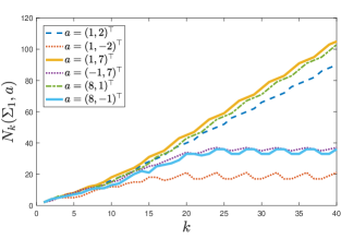
Figure 3: The number of extreme points $N_{k}(\Sigma_{1},a)$ given different initial vector $a$’s.

To prove the results in Table 1, we first introduce a few notations that will be used in the rest of this section. Given a pair $\Sigma$ of matrices and a vector $a\in\mathbb{R}^{2}$, we divide the set of extreme points $E_{k}(\Sigma,a)$ of $P_{k}(\Sigma,a)$ into five groups.

Definition 2.

Let $E^{i}_{k}(\Sigma,a)$ be the set of extreme points of $P_{k}(\Sigma,a)$ that are maximizers of the linear program $\max\{cx\mid x\in P_{k}(\Sigma,a)\}$ for some $c\in\mathrm{int}(\mathcal{Q}_{i})$, for $i=1,2,3,4$. Let $E^{0}_{k}(\Sigma,a)$ be the set of extreme points of $P_{k}(\Sigma,a)$ that are maximizers of the linear programs $\max\{cx\mid x\in P_{k}(\Sigma,a)\}$ where $c\in\{(1,0),(0,1),(-1,0),(0,-1)\}$.

Then

$$E_{k}(\Sigma,a)=\cup_{i=0}^{4}E^{i}_{k}(\Sigma,a)\text{ and }N_{k}(\Sigma,a)\leq\sum_{i=0}^{4}|E^{i}_{k}(\Sigma,a)|.$$ (8)

Example 3.

Figure 4 illustrates the polytopes $P_{k}(\Sigma_{3},a)$ and the sets of extreme points $E^{i}_{k}(\Sigma_{3},a)$ for $i\in[0:4]$ with $a=(2,1)^{\top}$, for $k=5$ and $k=7$.

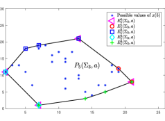
(a) $P_{5}(\Sigma_{3},(2,1)^{\top})$ and $E^{i}_{5}(\Sigma_{3},(2,1)^{\top})$

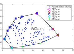
(b) $P_{7}(\Sigma_{3},(2,1)^{\top})$ and $E^{i}_{7}(\Sigma_{3},(2,1)^{\top})$

Figure 4: Examples of polytopes $P_{k}(\Sigma_{3},a)$ and associated sets of extreme points $E^{i}_{k}(\Sigma_{3},a)$ for $i\in[0:4]$.

5.1 $\Sigma_{1}=\{A_{1},A_{2}\}$

Proposition 7.

The pair $\Sigma_{1}$ has the oligo-vertex property and $N_{k}(\Sigma_{1})=O(k^{4})$.

Proposition 7 is an immediate consequence of the following propositions.

Proposition 8.

For any $a\in\mathrm{int}(\mathcal{Q}_{1})\cup\mathrm{int}(\mathcal{Q}_{3})$, $N_{k}(\Sigma_{1},a)=O(k^{2})$.

Proposition 9.

For any $a\in\partial{\mathcal{Q}_{1}}\cup\partial{\mathcal{Q}_{3}}$, $N_{k}(\Sigma_{1},a)=O(k^{2})$.

Proposition 10.

For any $a\in\mathrm{int}(\mathcal{Q}_{2})\cup\mathrm{int}(\mathcal{Q}_{4})$, $N_{k}(\Sigma_{1},a)=O(k^{4})$.

We first focus on proving Proposition 8. Our strategy is to bound the cardinality of $E^{i}_{k}(\Sigma_{1},a)$ for each $i$. Then according to (8), $N_{k}(\Sigma_{1})$ will be bounded as well.

Lemma 2.

For any $a\in\mathrm{int}(\mathcal{Q}_{1})$ and integer $k\geq 2$, $|E^{1}_{k}(\Sigma_{1},a)|\leq k+1$.

Proof.

To simplify the notations, we write $E^{1}_{k}$ and $P_{k}$ instead of $E^{1}_{k}(\Sigma_{1},a)$ and $P_{k}(\Sigma_{1},a)$ respectively in the rest of the proof. We claim that $|E_{k}^{1}|\leq|E_{k-1}^{1}|+1$ for $k\geq 2$. Then $|E_{k}^{1}|\leq|E_{1}^{1}|+(k-1)\leq 2+(k-1)=k+1$. To prove the claim, we first show that $E_{k}^{1}\subseteq A_{1}E_{k-1}^{1}\cup A_{2}E_{k-1}^{1}$. Note that

$$\max\{cx\mid x\in P_{k}\}=\max\{ \max\{cA_{1}x\mid x\in P_{k-1}\},\max\{cA_{2}x\mid x\in P_{k-1}\}\}.$$ (9)

Given $c\in\mathrm{int}(\mathcal{Q}_{1})$, both $cA_{1}$ and $cA_{2}$ are in the interior of $\mathcal{Q}_{1}$, so the maximizers of linear programs on the right are in the set $E_{k-1}^{1}$. Therefore, $E_{k}^{1}\subseteq A_{1}E_{k-1}^{1}\cup A_{2}E_{k-1}^{1}$.

Next we show that some points in $A_{1}E_{k-1}^{1}\cup A_{2}E_{k-1}^{1}$ cannot belong to $E_{k}^{1}$. Let $p=(p_{1},p_{2})^{\top}\in E_{k-1}^{1}$ be the maximizer of the linear program $\max\{x_{1}+x_{2}\mid x\in P_{k-1}\}$ with the smallest $x_{2}$-coordinate. Note that there is no other point in $E_{k-1}^{1}$ whose $x_{2}$-coordinate is $p_{2}$. Otherwise suppose that there is such a point $p^{\prime}$. The fact that $p$ is the maximizer of $\max\{x_{1}+x_{2}\mid x\in P_{k-1}\}$ implies $p_{1}>p^{\prime}_{1}$. Then $cp^{\prime}<cp$ for any $c\in\mathrm{int}(\mathcal{Q}_{1})$, which contradicts that $p^{\prime}\in E_{k-1}^{1}$. Now we can partition $E_{k-1}^{1}$ into three sets $S_{1}=\{x\mid x\in E_{k-1}^{1},x_{2}>p_{2}\}$, $S_{2}=\{p\}$, and $S_{3}=\{x\mid x\in E_{k-1}^{1},x_{2}<p_{2}\}$. Then $E_{k}^{1}\subseteq A_{1}S_{1}\cup A_{1}S_{2}\cup A_{1}S_{3}\cup A_{2}S_{1}\cup A_{2}S_{2}\cup A_{2}S_{3}$. We show below that the points in $A_{1}S_{1}$ or $A_{2}S_{3}$ cannot be in $E_{k}^{1}$.

First consider any point $x\in S_{1}$.

• If $x_{1}<x_{2}$, we have $cA_{2}x-cA_{1}x=c_{1}x_{1}+c_{2}(x_{2}-x_{1})>0$.

• Suppose $x_{1}\geq x_{2}$ and $c_{1}<c_{2}$. Since $x_{1}+x_{2}\leq p_{1}+p_{2}$, we have $x_{1}-p_{1}\leq p_{2}-x_{2}<0$. Therefore, $cA_{1}p-cA_{1}x=c_{1}(p_{2}-x_{2})+c_{2}(p_{1}-x_{1})\geq c_{1}(x_{1}-p_{1})+c_{2}(p_{1}-x_{1})=(c_{1}-c_{2})(x_{1}-p_{1})>0$.

• Suppose $x_{1}\geq x_{2}$ and $c_{1}\geq c_{2}$. Since $x_{1}+x_{2}\leq p_{1}+p_{2}$, $p_{2}-x_{1}\geq x_{2}-p_{1}$. Since $x_{1}\geq x_{2}>p_{2}$ and $x_{1}+x_{2}\leq p_{1}+p_{2}$, we have $p_{1}\geq x_{2}$. Then $cA_{2}p-cA_{1}x=c_{1}p_{1}+c_{1}(p_{2}-x_{2})+c_{2}(p_{2}-x_{1})\geq c_{1}p_{1}+c_{1}(p_{2}-x_{2})+c_{2}(x_{2}-p_{1})=(c_{1}-c_{2})(p_{1}-x_{2})+c_{1}p_{2}>0$.

Therefore, $A_{1}x\in A_{1}S_{1}$ cannot be a maximizer of linear program (9) with $c\in\mathrm{int}(\mathcal{Q}_{1})$.

Now consider any point $x\in S_{3}$. Since $p_{2}-x_{2}>0$ and $p_{1}+p_{2}\geq x_{1}+x_{2}$, $cA_{2}p-cA_{2}x=c_{1}(p_{1}+p_{2}-x_{1}-x_{2})+c_{2}(p_{2}-x_{2})>0$. Therefore, $A_{2}x\in A_{2}S_{3}$ cannot be a maximizer of linear program (9) with $c\in\mathrm{int}(\mathcal{Q}_{1})$. Hence, $|E_{k}^{1}|\leq|A_{1}S_{2}|+|A_{1}S_{3}|+|A_{2}S_{1}|+|A_{2}S_{2}|=|S_{1}|+|S_{2}|+|S_{3}|+|S_{2}|=|E_{k-1}^{1}|+1$. ∎

Lemma 3.

For any $a\in\mathrm{int}(\mathcal{Q}_{1})$ and integer $k\geq 2$, $|E_{k}^{3}(\Sigma_{1},a)|\leq 2$.

Proof.

To simplify the notations, we write $E_{k}^{3}$ instead of $E_{k}^{3}(\Sigma_{1},a)$ in the rest of the proof. Let $a=(a_{1},a_{2})^{\top}\in\mathrm{int}(\mathcal{Q}_{1})$. Assume that $a_{1}\leq a_{2}$. The case in which $a_{1}>a_{2}$ can be proved similarly. We show below by induction that $E_{k}^{3}\subseteq\{A_{1}^{k}a,A_{1}^{k-2}A_{2}A_{1}a\}$ for any $k\geq 2$. For the base case $k=2$, given any $c\in\mathrm{int}(\mathcal{Q}_{3})$, $cA_{1}^{2}a-cA_{2}^{2}a=-2c_{1}a_{2}>0,cA_{1}^{2}a-cA_{1}A_{2}a=c_{1}(a_{1}-a_{2})-c_{2}a_{1}>0$. Hence, $E_{2}^{3}\subseteq\{A_{1}^{2}a,A_{2}A_{1}a\}$.

Now suppose that $E_{t}^{3}\subseteq\{A_{1}^{t}a,A_{1}^{t-2}A_{2}A_{1}a\}$ for some $t\geq 2$. We want to show that $E_{t+1}^{3}\subseteq\{A_{1}^{t+1}a,A_{1}^{t-1}A_{2}A_{1}a\}$. We assume that $t$ is even (a similar argument can be used to prove the result when $t$ is odd). Similar to the proof of (9) in Lemma 2, we have $E_{k}^{3}\subseteq A_{1}E_{k-1}^{3}\cup A_{2}E_{k-1}^{3}$ for $k\geq 2$. Then by the induction hypothesis, we have $E_{t+1}^{3}\subseteq\{A_{1}^{t+1}a,A_{1}^{t-1}A_{2}A_{1}a,A_{2}A_{1}^{t}a,A_{2}A_{1}^{t-2}A_{2}A_{1}a\}$. Since $t$ is even, $A_{1}^{t}a=a$ and $A_{1}^{t-2}A_{2}A_{1}a=(a_{1}+a_{2},a_{1})^{\top}$. For any $c\in\mathrm{int}(\mathcal{Q}_{3})$, $cA_{1}^{t+1}a-cA_{2}A_{1}^{t}a=-c_{1}a_{1}+c_{2}(a_{1}-a_{2})>0$, and $cA_{1}^{t+1}a-cA_{2}A_{1}^{t-2}A_{2}A_{1}a=-2c_{1}a_{1}>0$.

Hence, $E_{t+1}^{3}\subseteq\{A_{1}^{t+1}a,A_{1}^{t-1}A_{2}A_{1}a\}$. We conclude that $|E_{k}^{3}|\leq 2$ for any integer $k\geq 2$. ∎

Lemma 4.

For any $a\in\mathrm{int}(\mathcal{Q}_{1})$ and integer $k\geq 2$, $|E_{k}^{4}(\Sigma_{1},a)|\leq|E_{k-1}^{4}(\Sigma_{1},a)|+|E_{k-1}^{1}(\Sigma_{1},a)|+2$ and $|E_{k}^{2}(\Sigma_{1},a)|\leq|E_{k-1}^{4}(\Sigma_{1},a)|$.

Proof.

To simplify the notations, we omit the dependence of $\Sigma_{1}$ and $a$ in the rest of the proof. We first prove that $|E_{k}^{4}|\leq|E_{k-1}^{4}|+|E_{k-1}^{1}|+2$. Note that

$$\max\{cx\mid x\in P_{k}\}=\max\{ \max\{cA_{1}A_{1}x\mid x\in P_{k-2}\},\max\{cA_{1}A_{2}x\mid x\in P_{k-2}\},$$

$$\max\{cA_{2}A_{1}x\mid x\in P_{k-2}\},\max\{cA_{2}A_{2}x\mid x\in P_{k-2}\}\}.$$

Since $P_{k-2}\subseteq\mathrm{int}(\mathcal{Q}_{1})$, for any $c$ with $c_{1}>0$ and $c_{2}<0$ and $x\in P_{k-2}$, $cA_{2}^{2}x=(c_{1},2c_{1}+c_{2})x>(c_{1},c_{2})x=cA_{1}^{2}x,cA_{2}^{2}x=(c_{1},2c_{1}+c_{2})x>(c_{2},c_{1}+c_{2})x=cA_{1}A_{2}x$. Therefore, $\max\{cx\mid x\in P_{k}\}=\max\{\max\{cA_{2}A_{1}x\mid x\in P_{k-2}\},\max\{cA_{2}A_{2}x\mid x\in P_{k-2}\}\}=\max\{cA_{2}x\mid x\in P_{k-1}\}$. Now that $cA_{2}=(c_{1},c_{1}+c_{2})$ is a vector in the first or the fourth quadrant, the maximizers of $\max\{cx\mid x\in P_{k}\}$ must be in $A_{2}E_{k-1}^{1}\cup A_{2}E_{k-1}^{4}\cup A_{2}S$, where $S$ is the set of extreme points of $P_{k-1}$ that are maximizers of $\max\{x_{1}\mid x\in P_{k-1}\}$. Therefore, $|E_{k}^{4}|\leq|A_{2}E_{k-1}^{4}|+|A_{2}E_{k-1}^{1}|+|A_{2}S|\leq|E_{k-1}^{4}|+|E_{k-1}^{1}|+2$.

To prove that $|E_{k}^{2}|\leq|E_{k-1}^{4}|$, consider $c=(c_{1},c_{2})$ with $c_{1}<0$ and $c_{2}>0$. For any $x\in P_{k-2}$,

$$cA_{1}A_{2}x =(c_{2},c_{1}+c_{2})x>(c_{1}+c_{2},c_{1})x=cA_{2}A_{1}x,$$

$$cA_{1}A_{2}x =(c_{2},c_{1}+c_{2})x>(c_{1},2c_{1}+c_{2})x=cA_{2}A_{2}x.$$

Thus we have $\max\{cx\mid x\in P_{k}\}=\max\{\max\{cA_{1}A_{1}x\mid x\in P_{k-2}\},\max\{cA_{1}A_{2}x\mid x\in P_{k-2}\}\}=\max\{cA_{1}x\mid x\in P_{k-1}\}$. Since $cA_{1}=(c_{2},c_{1})$ is a vector in the interior of the fourth quadrant, the optimal solutions of $\max\{cx\mid x\in P_{k}\}$ must be in $A_{1}E_{k-1}^{4}$. Therefore, $|E_{k}^{2}|\leq|E_{k-1}^{4}|$. ∎

Now we are ready to prove Proposition 8,

Proof of Proposition 8.

We only need to prove the case where $a\in\mathrm{int}(\mathcal{Q}_{1})$. When $a\in\mathrm{int}(\mathcal{Q}_{3})$, it is easy to verify that $N_{k}(\Sigma_{1},a)=N_{k}(\Sigma_{1},-a)$. By Lemma 2 and Lemma 3, we have $|E_{k}^{1}(\Sigma_{1},a)|\leq k+1$ and $|E_{k}^{3}(\Sigma_{1},a)|\leq 2$ for any $a\in\mathrm{int}(\mathcal{Q}_{1})$ and integer $k\geq 2$. By Lemma 4, for any $a\in\mathrm{int}(\mathcal{Q}_{1})$ and integer $k\geq 3$, $|E_{k}^{4}(\Sigma_{1},a)|\leq|E_{k-1}^{4}(\Sigma_{1},a)|+|E_{k-1}^{1}(\Sigma_{1},a)|+2\leq|E_{k-1}^{4}(\Sigma_{1},a)|+(k+2)\leq|E_{2}^{4}(\Sigma_{1},a)|+\sum_{i=2}^{k-1}(i+3)\leq\frac{1}{2}k^{2}+\frac{5}{2}k-3$, and $|E_{k}^{2}(\Sigma_{1},a)|\leq|E_{k-1}^{4}(\Sigma_{1},a)|\leq\frac{1}{2}k^{2}+\frac{3}{2}k-5$. Therefore, $N_{k}(\Sigma_{1},a)\leq|E_{k}^{1}(\Sigma_{1},a)|+|E_{k}^{2}(\Sigma_{1},a)|+|E_{k}^{3}(\Sigma_{1},a)|+|E_{k}^{4}(\Sigma_{1},a)|+|E_{k}^{0}(\Sigma_{1},a)|=O(k^{2})$. ∎

The conclusion $N_{k}(\Sigma_{1},a)=O(k^{2})$ can be easily extended to the case where $a$ is on the boundary of the first or third quadrant.

Proof of Proposition 9.

We only need to prove the case where $a\in\partial{\mathcal{Q}_{1}}$. The case where $a\in\partial{\mathcal{Q}_{3}}$ follows from the fact $N_{k}(\Sigma_{1},a)=N_{k}(\Sigma_{1},-a)$. We first prove the result when $a$ is on the positive $x_{1}$-axis. Without loss of generality, assume that $a=(1,0)^{\top}$. We claim that for any integer $k\geq 3$,

$$X_{k}(\Sigma_{1},(1,0)^{\top})=X_{k-2}(\Sigma_{1},(1,1)^{\top})\cup\{(1,0)^{\top},(0,1)^{\top}\}.$$

To see this, consider any value of $x(k)$ in $X_{k}(\Sigma_{1},(1,0)^{\top})$ that is different from $(1,0)^{\top}$ and $(0,1)^{\top}$. Since $A_{1}^{t}a=(0,1)^{\top}$ for odd integer $t\geq 1$, $A_{1}^{t}a=(1,0)^{\top}$ for even integer $t\geq 1$, $A_{2}^{t}a=(1,0)^{\top}$ for any integer $t\geq 1$, and $A_{2}A_{1}a=(1,1)^{\top}$. For $x(k)$ to take a value different from $(0,1)^{\top}$ and $(1,0)^{\top}$, $x(k)$ must be in the form of $T_{k-1}\cdots T_{l}x(l)$ with $T_{j}\in\Sigma_{1}$ for $j\in[l:k-1]$ and $x(l)=(1,1)^{\top}$ for some $l\geq 2$. But when $x(l)=(1,1)^{\top}$, we have $A_{1}^{j}x(l)=x(l)$ for any integer $j\geq 1$. Then $x(k)=T_{k-1}\cdots T_{l}A_{1}^{l-2}x(l)$, which is a point in $X_{k-2}(\Sigma_{1},(1,1)^{\top})$. Thus $X_{k}(\Sigma_{1},(1,0)^{\top})\subseteq X_{k-2}(\Sigma_{1},(1,1)^{\top})\cup\{(1,0)^{\top},(0,1)^{\top}\}$. On the other hand, given a point in $X_{k-2}(\Sigma_{1},(1,1)^{\top})$ written in the form of $T_{k-3}\cdots T_{0}(1,1)^{\top}$ with $T_{j}\in\Sigma_{1}$ for $j\in[0:k-3]$, we can also write it in the form of $T_{k-3}\cdots T_{0}A_{2}A_{1}(1,0)^{\top}$. Thus $X_{k}(\Sigma_{1},(1,0)^{\top})\supseteq X_{k-2}(\Sigma_{1},(1,1)^{\top})\cup\{(1,0)^{\top},(0,1)^{\top}\}$. Therefore, $N_{k}(\Sigma_{1},(1,0)^{\top})\leq N_{k-2}(\Sigma_{1},(1,1)^{\top})+2=O(k^{2})$. The last equality follows from Proposition 8. The case where $a$ is on the positive $x_{2}$-axis can be proved similarly. ∎

We proceed to prove Proposition 10. Let $X^{2,4}_{k}(\Sigma_{1},a)$ be the set of points in $X_{k}(\Sigma_{1},a)$ that are in the interior of the second or fourth quadrant, i.e.,

$$X^{2,4}_{k}(\Sigma_{1},a)=X_{k}(\Sigma_{1},a)\cap(\mathrm{int}(\mathcal{Q}_{2})\cup\mathrm{int}(\mathcal{Q}_{4})).$$

Lemma 5.

For any $a\in\mathrm{int}(\mathcal{Q}_{4})$ and integer $k\geq 2$, $X^{2,4}_{k}(\Sigma_{1},a)$ contains no more than $4k+4$ points.

Proof.

Without loss of generality, assume $a=(1,a_{2})^{\top}$ with $a_{2}<0$. Let $u_{0}=\max\{1,-a_{2}\}$ and $v_{0}=\min\{1,-a_{2}\}$. Define the following sequence of non-negative numbers recursively: $u_{j}=\max\{v_{j-1},u_{j-1}-v_{j-1}\}$ and $v_{j}=\min\{v_{j-1},u_{j-1}-v_{j-1}\}$ for $j\in[1:k]$. For each $t\in[0:k]$, define $S_{t}=\{(u_{t},-v_{t})^{\top},(-u_{t},v_{t})^{\top},(v_{t},-u_{t})^{\top},(-v_{t},u_{t})^{\top}\}$.

Given any $s^{k}\in X^{2,4}_{k}(\Sigma_{1},a)$, assume that $s^{k}=T_{k-1}\cdots T_{0}a$ with $T_{j}\in\Sigma_{1}$ for $j\in[0:k-1]$. We claim that for any integer $k\geq 0$, if $t$ out of the $k$ matrices $T_{0},\cdots,T_{k-1}$ are $A_{2}$, then $s^{k}\in S_{t}$. We prove the claim by induction on $k$. First consider the base case $k=0$. If $|a_{2}|\geq 1$, then $u_{0}=-a_{2}$ and $v_{0}=1$, so $s^{k}=a=(v_{0},-u_{0})^{\top}\in S_{0}$. If $|a_{2}|<1$, then $u_{0}=1$ and $v_{0}=-a_{2}$, so $s^{k}=a=(u_{0},-v_{0})^{\top}\in S_{0}$. Now suppose that the claim holds for integer $k=l\geq 0$. Specifically, $s^{l}=T_{l-1}\cdots T_{0}a\in S_{t}$ if $t\in[0:l]$ out of the $l$ matrices $T_{0},\cdots,T_{l-1}$ are $A_{2}$. We want to prove that any point $s^{l+1}=T_{l+1}\cdots T_{0}a$ in $X^{2,4}_{l+1}(\Sigma_{1},a)$ also belongs to $S_{t}$, if $t\in[0:l+1]$ out of the $l+1$ matrices $T_{0},\cdots,T_{l+1}$ are $A_{2}$. If $T_{l+1}=A_{1}$, then $t$ out of the $l$ matrices $T_{l},\ldots,T_{0}$ are $A_{2}$. Based on the induction hypothesis, the point $s=T_{l}\cdots T_{0}a\in S_{t}$. Since $A_{1}S_{t}=S_{t}$, $s^{l+1}=A_{1}s$ must be in $S_{t}$ as well. If $T_{l+1}=A_{2}$, then $(t-1)$ out of the $l$ matrices $T_{l},\ldots,T_{0}$ are $A_{2}$. Based on the induction hypothesis, the point $s=T_{l}\cdots T_{0}a\in S_{t-1}$. The set $S_{t}$ contains four points. We consider one case $s=(u_{t-1},-v_{t-1})^{\top}$ here, and the result for the other cases can be proved similarly. We have $s^{l+1}=A_{2}s=(u_{t-1}-v_{t-1},-v_{t-1})^{\top}$. Since $s^{l+1}$ is in the interior of second or fourth quadrant and $-v_{t-1}<0$, we must have $u_{t-1}-v_{t-1}>0$. If $v_{t-1}\geq u_{t-1}-v_{t-1}$, then $u_{t}=v_{t-1}$, $v_{t}=u_{t-1}-v_{t-1}$, and $s^{l+1}=(v_{t},-u_{t})^{\top}\in S_{t}$. If $v_{t-1}<u_{t-1}-v_{t-1}$, then $u_{t}=u_{t-1}-v_{t-1}$, $v_{t}=v_{t-1}$, and $s^{l+1}=(u_{t},-v_{t})^{\top}\in S_{t}$. With the claim, we conclude that $X^{2,4}_{k}(\Sigma_{1},a)$ contains at most $4k+4$ different points. ∎

Proof of Proposition 10.

We omit the dependence of $\Sigma_{1}$ in the rest of the proof to simplify the notation. Given a set $S\subseteq\mathbb{R}^{2}$, define $X_{k}(S)=\cup_{a\in S}X_{k}(a)$.

First note that for any $x$ in the first (third) quadrant, $A_{1}x$ and $A_{2}x$ are both in the first (third) quadrant. Thus the points in $X^{2,4}_{i+1}(a)$ can only be linear transformations of points in $X^{2,4}_{i}(a)$ under $A_{1}$ or $A_{2}$. In addition, for any $x$ in the second or fourth quadrant, $A_{1}x$ is also in the second or fourth quadrant. Therefore, for any integer $i\geq 0$, $A_{1}X^{2,4}_{i}(a)\cup A_{2}X^{2,4}_{i}(a)=X^{2,4}_{i+1}(a)\cup(A_{2}X^{2,4}_{i}(a)\cap(\mathcal{Q}_{1}\cup\mathcal{Q}_{3}))$. Given any $a$ in the interior of the second quadrant, we have

$$\begin{split}X_{k}(a)=&X_{k}(X^{2,4}_{0}(a))=X_{k-1}(A_{1}X^{2,4}_{0}(a)\cup A_{2}X^{2,4}_{0}(a))\\ =&X_{k-1}(X^{2,4}_{1}(a))\cup X_{k-1}(A_{2}X^{2,4}_{0}(a)\cap(\mathcal{Q}_{1}\cup\mathcal{Q}_{3}))\\ =&(X_{k-2}(X^{2,4}_{2}(a))\cup X_{k-2}(A_{2}X^{2,4}_{1}(a)\cap(\mathcal{Q}_{1}\cup\mathcal{Q}_{3})))\\ &\cup X_{k-1}(A_{2}X^{2,4}_{0}(a)\cap(\mathcal{Q}_{1}\cup\mathcal{Q}_{3}))\\ &\qquad\cdots\\ =&X_{l}(X^{2,4}_{k-l}(a))\cup\cup_{j=l}^{k-1}X_{j}(A_{2}X^{2,4}_{k-1-j}(a)\cap(\mathcal{Q}_{1}\cup\mathcal{Q}_{3}))\end{split}$$ (10)

for any $l\geq 1$.

On the other hand, for any $x$ in the first or third quadrant, we have shown that there exists some integer $k_{0}$ and $\alpha>0$ such that $N_{k}(x)\leq\alpha k^{2}$ for any integer $k\geq k_{0}$. Setting $l=k_{0}$ in equation (10) we have $X_{k}(a)=X_{k_{0}}(X^{2,4}_{k-k_{0}}(a))\cup\cup_{j=k_{0}}^{k-1}X_{j}(A_{2}X^{2,4}_{k-1-j}(a)\cap(\mathcal{Q}_{1}\cup\mathcal{Q}_{3}))$. Therefore,

$$N_{k}(a) \leq|X_{k_{0}}(X^{2,4}_{k-k_{0}}(a))|+\sum_{j=k_{0}}^{k-1}\sum_{x\in A_{2}X^{2,4}_{k-1-j}(a)\cap(\mathcal{Q}_{1}\cup\mathcal{Q}_{3})}N_{j}(x)$$

$$\leq\sum_{x\in X^{2,4}_{k-k_{0}}(a)}|X_{k_{0}}(x)|+\sum_{j=k_{0}}^{k-1}|A_{2}X^{2,4}_{k-1-j}(a)|\alpha j^{2}$$

$$\leq|X^{2,4}_{k-k_{0}}(a)|2^{k_{0}}+\sum_{j=k_{0}}^{k-1}|X^{2,4}_{k-1-j}(a)|\cdot\alpha j^{2}$$

$$\leq(4k-4k_{0}+4)2^{k_{0}}+\sum_{j=k_{0}}^{k-1}(4k-4j)\alpha j^{2}\leq\beta k^{4},$$

for some constant $\beta$. The second last inequality follows from Lemma 5. Therefore $N_{k}(a)=O(k^{4})$. ∎

5.2 $\Sigma_{2}=\{A_{1},A_{4}\}$

In this section, we will prove that $N_{k}(\Sigma_{2})=O(k)$.

Lemma 6.

Given any polytope $P\subseteq\mathbb{R}\times\mathbb{R}_{+}$ or $P\subseteq\mathbb{R}\times\mathbb{R}_{-}$, the number of extreme points of $\mathrm{conv}(P\cup A_{2}P)$ is at most two more than the number of extreme points of $P$.

Proof.

We first prove the case in which $P\subseteq\mathbb{R}\times\mathbb{R}_{+}$. The result is easy to show if $P$ is a singleton or a line segment. Now suppose $P$ is full dimensional. Let $r=(r_{1},r_{2})^{\top}$ be the extreme point of $P$ with the largest $x_{2}$-coordinate; if there are two such extreme points, let $r$ be the one with a larger $x_{1}$-coordinate. Similarly, let $s=(s_{1},s_{2})^{\top}$ be the extreme point of $P$ with the smallest $x_{2}$-coordinate; let $s$ be the one with a larger $x_{1}$-coordinate if there are two such extreme points. Divide the extreme points of $P$ other than $r$ and $s$ into two sets: (1) Set $Q_{1}$ consisting of extreme points visited if we walk clockwise along the boundary of $P$ from $s$ to $r$; (2) Set $Q_{2}$ consisting of extreme points visited if we walk clockwise along the boundary of $P$ from $r$ to $s$. Let $R=\{r,s,A_{2}r,A_{2}s\}$. Since $\mathrm{ext}(P)=Q_{1}\cup Q_{2}\cup\{r,s\}$, the possible extreme points of $\mathrm{conv}(P\cup A_{2}P)$ are among $Q_{1}$, $Q_{2}$, $A_{2}Q_{1}$, $A_{2}Q_{2}$, and $R$.

We claim that any point in $Q_{2}$ can be represented as a convex combination of points in $Q_{1}\cup A_{2}Q_{2}\cup R$. To see this, first consider any point $p=(p_{1},p_{2})^{\top}\in Q_{2}$. By the definition of $Q_{2}$, we have $p_{2}>0$ and there exists a point $h=(h_{1},h_{2})^{\top}$ on the line segment connecting $r$ and $s$ such that $h_{1}<p_{1}$ and $h_{2}=p_{2}$. See the illustration in Figure 5. We can verify that $p=\lambda A_{2}p+(1-\lambda)h$ with $\lambda=\frac{p_{1}-h_{1}}{p_{1}+p_{2}-h_{1}}\in(0,1)$. Thus $p$ can be represented as a convex combination of $A_{2}p$ and $h$. Since $h$ can also be represented by a convex combination of $r$ and $s$, $p$ can be represented as a convex combination of $A_{2}p$, $r$, and $s$. Therefore, we show that any point in $Q_{2}$ is a convex combination of points in $Q_{1}\cup A_{2}Q_{2}\cup R$.

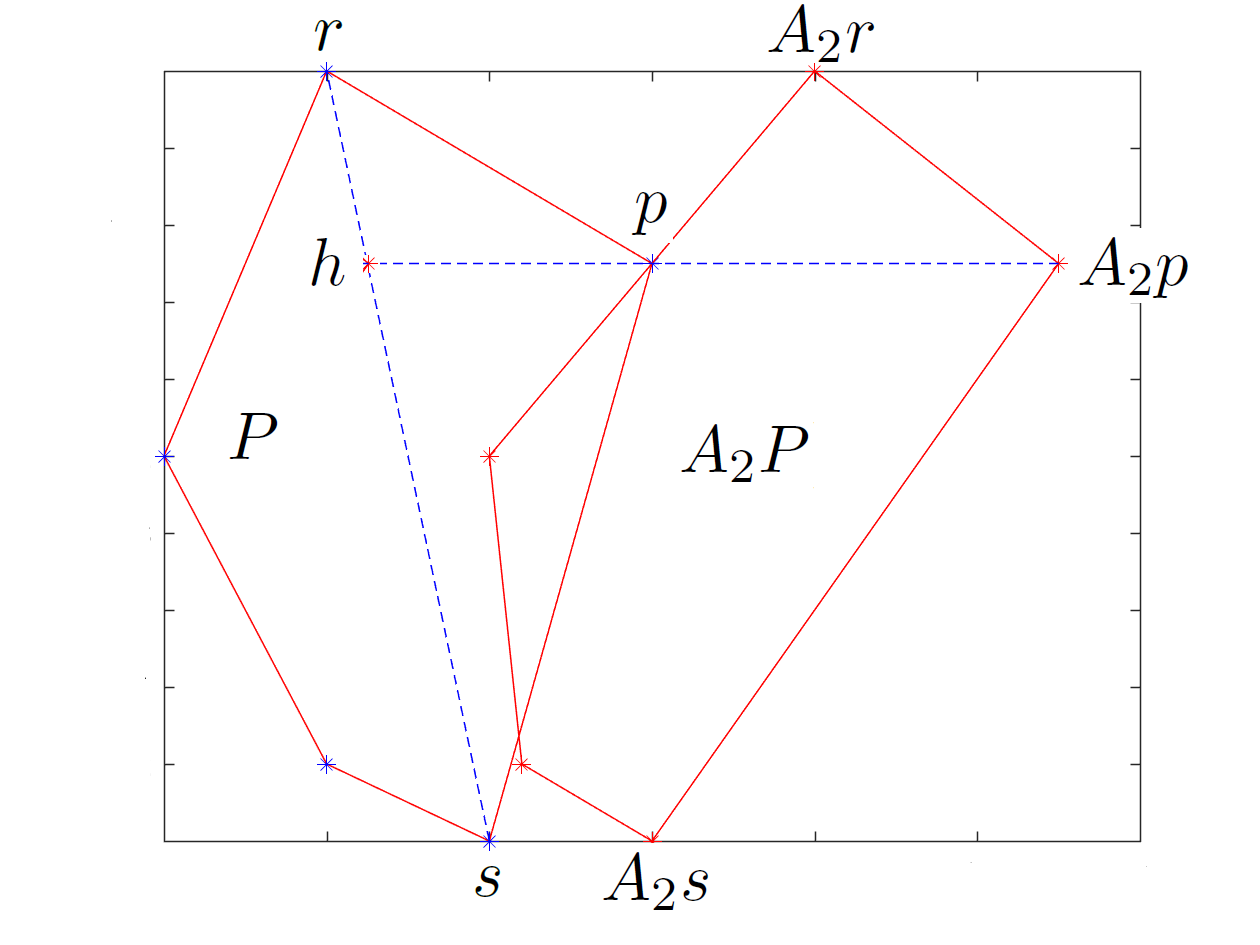
Figure 5: Point $p$ is a convex combination of $r$, $s$, and $A_{2}p$.

Similarly, we can show that any point in $A_{2}Q_{1}$ is a convex combination of points in $Q_{1}\cup A_{2}Q_{2}\cup R$. Then we have $\mathrm{conv}(P\cup A_{2}P)=\mathrm{conv}(Q_{1}\cup A_{2}Q_{2}\cup R)$. Thus $|\mathrm{ext}(\mathrm{conv}(P\cup A_{2}P))|=|\mathrm{ext}(\mathrm{conv}(Q_{1}\cup A_{2}Q_{2}\cup R))|\leq|Q_{1}|+|A_{2}Q_{2}|+|R|\leq(|Q_{1}|+|Q_{2}|+|\{r,s\}|)+2\leq|\mathrm{ext}(P)|+2$. The result for any $P\subseteq\mathbb{R}\times\mathbb{R}_{-}$ can be proved similarly. ∎

Proposition 11.

The pair $\Sigma_{2}$ has the oligo-vertex property and $N_{k}(\Sigma_{2})=O(k)$.

Proof.

To simplify the notation, we omit the dependence of $\Sigma_{2}$ in $N_{k}(\Sigma_{2},a)$ and $P_{k}(\Sigma_{2},a)$ in the rest of this proof. We claim that $N_{k+1}(a)\leq N_{k}(a)+8$ for any $a\in\mathbb{R}^{2}$ and integer $k\geq 2$. Then $N_{k}(a)\leq N_{k-1}(a)+8\leq\cdots\leq N_{2}(a)+8(k-2)\leq 4+8(k-2)=8k-12$. Thus $N_{k}=O(k)$.

To prove the claim, first observe that $P_{k+1}(a)=\mathrm{conv}(A_{1}P_{k}(a)\cup A_{4}P_{k}(a))=\mathrm{conv}(A_{1}P_{k}(a)\cup A_{2}A_{1}P_{k}(a))$. Define $P^{+}=A_{1}P_{k}(a)\cap\{x\mid x_{2}\geq 0\}$ and $P^{-}=A_{1}P_{k}(a)\cap\{x\mid x_{2}\leq 0\}$. Notice that $P^{+}$ is a polytope in $\mathbb{R}\times\mathbb{R}_{+}$ and $P^{-}$ is polytope in $\mathbb{R}\times\mathbb{R}_{-}$, and $|\mathrm{ext}(P^{+})|+|\mathrm{ext}(P^{-})|\leq|\mathrm{ext}(A_{1}P_{k}(a))|+4=N_{k}(a)+4$. The first inequality above follows from the fact the line $x_{2}=0$ may introduce two new extreme points for both $P^{+}$ and $P^{-}$. On the other hand,

$$P_{k+1}(a) =\mathrm{conv}(A_{1}P_{k}(a)\cup A_{2}A_{1}P_{k}(a))$$

$$=\mathrm{conv}(P^{+}\cup P^{-}\cup A_{2}(P^{+}\cup P^{-}))$$

$$=\mathrm{conv}(\mathrm{conv}(P^{+}\cup A_{2}P^{+})\cup\mathrm{conv}(P^{-}\cup A_{2}P^{-})).$$

Thus $N_{k+1}(a)\leq|\mathrm{ext}(\mathrm{conv}(\mathrm{conv}(P^{+}\cup A_{2}P^{+})))|+|\mathrm{ext}(\mathrm{conv}(P^{-}\cup A_{2}P^{-}))|$. By Lemma 6, $|\mathrm{ext}(\mathrm{conv}(P^{+}\cup A_{2}P^{+}))|\leq|\mathrm{ext}(P^{+})|+2$ and $|\mathrm{ext}(\mathrm{conv}(P^{-}\cup A_{2}P^{-}))|\leq|\mathrm{ext}(P^{-})|+2$. Thus we have $N_{k+1}(a)\leq|\mathrm{ext}(\mathrm{conv}(P^{+}))|+2+|\mathrm{ext}(\mathrm{conv}(P^{-}))|+2\leq N_{k}(a)+8$. ∎

5.3 $\Sigma_{3}=\{A_{2},A_{3}\}$

We first prove the following result when the initial vector $a$ is in the first quadrant.

Proposition 12.

For any $a\in\mathcal{Q}_{1}$, $N_{k}(\Sigma_{3},a)=O(k)$.

Proof.

The proof is similar to the proof of Proposition 8 for $\Sigma_{1}$. We first bound the cardinality of $E_{k}^{i}(\Sigma_{3},a)$ for each $i$. Similar to the proofs of Lemmas 2, 3, and 4, we can show that for any $a\in\mathcal{Q}_{1}$, $|E^{1}_{k}(\Sigma_{3},a)|\leq 4$ when $k\geq 3$, $E^{3}_{k}(\Sigma_{3},a)\subseteq\{A_{2}^{k}a,A_{3}^{k}a\}$ when $k\geq 1$, $|E^{4}_{k}(\Sigma_{3},a)|\leq|E^{4}_{k-1}(\Sigma_{3},a)|+|E^{1}_{k-1}(\Sigma_{3},a)|+2$ and $|E^{2}_{k}(\Sigma_{3},a)|\leq|E^{2}_{k-1}(\Sigma_{3},a)|+|E^{1}_{k-1}(\Sigma_{3},a)|+2$ when $k\geq 1$, respectively. Then $|E^{4}_{k}(\Sigma_{3},a)|\leq|E^{4}_{k-1}(\Sigma_{3},a)|+6\leq|E^{4}_{3}(\Sigma_{3},a)|+6(k-3)\leq 6k-10$. Similarly, $|E^{2}_{k}(\Sigma_{3},a)|\leq 6k-10$. Finally, for any $a\in\mathcal{Q}_{1}$ and integer $k\geq 3$, $N_{k}(\Sigma_{3},a)\leq\sum_{i=0}^{4}|E^{i}_{k}(\Sigma_{3},a)|\leq 8+4+(6k-10)+2+(6k-10)+8=12k-6$. ∎

Proposition 13.

The pair $\Sigma_{3}$ has the oligo-vertex property and $N_{k}(\Sigma_{3})=O(k^{2})$.

Proof.

We only need to prove that $N_{k}(\Sigma_{3},a)=O(k^{2})$ for any $a\in\mathrm{int}(\mathcal{Q}_{4})$. Define $f_{k}=\sup\{N_{k}(\Sigma_{3},a)\mid a\in\mathrm{int}(\mathcal{Q}_{4})\}$ for any integer $k\geq 1$. Note that $f_{k}=\sup\{N_{k}(\Sigma_{3},a)\mid a\in\mathrm{int}(\mathcal{Q}_{2})\}$ for $k\geq 1$ as well. Since $P_{k}(\Sigma_{3},a)=\mathrm{conv}(P_{k-1}(\Sigma_{3},A_{2}a)\cup P_{k-1}(\Sigma_{3},A_{3}a))$, we have $N_{k}(\Sigma_{3},a)\leq N_{k-1}(\Sigma_{3},A_{2}a)+N_{k-1}(\Sigma_{3},A_{3}a)$. Consider a vector $a=(a_{1},a_{2})^{\top}\in\mathrm{int}(\mathcal{Q}_{4})$ with $a_{1}>0$ and $a_{2}<0$.

1. If $a_{1}=-a_{2}$, we have $A_{2}a=(0,a_{2})^{\top}\in\mathcal{Q}_{3}$ and $A_{3}a=(a_{1},0)^{\top}\in\mathcal{Q}_{1}$. Then there exists $\alpha>0$ and integer $k_{0}$ such that for any integer $l\geq k_{0}$, $N_{l}(\Sigma_{3},A_{2}a)\leq\alpha l$ and $N_{l}(\Sigma_{3},A_{3}a)\leq\alpha l$. Thus for any integer $k\geq k_{0}+1$, $N_{k}(\Sigma_{3},a)\leq N_{k-1}(\Sigma_{3},A_{2}a)+N_{k-1}(\Sigma_{3},A_{3}a)\leq\alpha(k-1)+\alpha(k-1)\leq 2\alpha k$. Therefore, $N_{k}(\Sigma_{3},a)=O(k)$.

2. If $a_{1}<-a_{2}$, we have $A_{2}a=(a_{1}+a_{2},a_{2})^{\top}\in\mathcal{Q}_{3}$ and $A_{3}a=(a_{1},a_{1}+a_{2})^{\top}\in\mathrm{int}(\mathcal{Q}_{4})$. Then there exists $\alpha>0$ and integer $k_{0}$ such that for any integer $l\geq k_{0}$, $N_{l}(\Sigma_{3},A_{2}a)\leq\alpha l$. For any $k\geq k_{0}+1$, $N_{k}(\Sigma_{3},a)\leq N_{k-1}(\Sigma_{3},A_{2}a)+N_{k-1}(\Sigma_{3},A_{3}a)\leq\alpha(k-1)+f_{k-1}$. Then for any $k\geq k_{0}+1$, $f_{k}\leq\alpha(k-1)+f_{k-1}$. Thus for any $k\geq 2k_{0}$,

   $$f_{k} \leq\alpha(k-1)+f_{k-1}\leq\alpha(k-1)+\alpha(k-2)+f_{k-2}$$

   $$\qquad\cdots\leq\alpha(k-1)+\alpha(k-2)+\cdots+\alpha k_{0}+f_{k_{0}}$$

   $$\leq\alpha\frac{(k-1+k_{0})(k-k_{0})}{2}+2^{k_{0}}\leq\beta k^{2},$$

   for some $\beta>0$. Therefore, $f_{k}=O(k^{2})$.

3. If $a_{1}>-a_{2}$, it can be proved that $f_{k}=O(k^{2})$ with a similar argument as in the case $a_{1}<-a_{2}$.

∎

5.4 $\Sigma_{4}=\{A_{4},A_{5}\}$

Proposition 14.

The pair $\Sigma_{4}$ has the oligo-vertex property and $N_{k}(\Sigma_{4})=O(k^{2})$.

Proof.

First observe that $A_{4}A_{5}=A_{2}A_{2}$, $A_{4}A_{4}=A_{2}A_{3}$, $A_{5}A_{5}=A_{3}A_{2}$, and $A_{5}A_{4}=A_{3}A_{3}$. When $k$ is an even integer, every product of $k$ matrices with $A_{2}$ and $A_{3}$ can be represented by a product of $k$ matrices with $A_{4}$ and $A_{5}$ and vice versa. Therefore, for any given $a\in\mathbb{R}^{2}$, $P_{k}(\Sigma_{4},a)=P_{k}(\Sigma_{3},a)$ and $N_{k}(\Sigma_{4},a)=N_{k}(\Sigma_{3},a)$. When $k$ is an odd integer, $P_{k}(\Sigma_{4},a)=\mathrm{conv}(A_{4}P_{k-1}(\Sigma_{4},a)\cup A_{5}P_{k-1}(\Sigma_{4},a))$ and $N_{k}(\Sigma_{4},a)\leq 2N_{k-1}(\Sigma_{4},a)=2N_{k-1}(\Sigma_{3},a)$. Since there exists $\alpha>0$ and integer $k_{0}$ such that $N_{k}(\Sigma_{3},a)\leq\alpha k^{2}$ for any integer $k\geq k_{0}$, we have $N_{k}(\Sigma_{4},a)\leq 2\alpha k^{2}$ for any integer $k\geq k_{0}$. Therefore, $N_{k}(\Sigma_{4})=O(k^{2})$. ∎

5.5 $\Sigma_{5}=\{A_{2},A_{4}\}$

Proposition 15.

For any $a\in\mathcal{Q}_{1}$ with $a_{1}\geq a_{2}$, $N_{k}(\Sigma_{5},a)=O(k)$.

Proof.

First similar to the proofs of Lemmas 2, 3, and 4, we can show by induction that for any $a\in\mathcal{Q}_{1}$ with $a_{1}\geq a_{2}$, $E^{1}_{k}(\Sigma_{5},k)=\{A_{4}^{k}a\}$ and $E^{3}_{k}(\Sigma_{5},a)=\{A_{2}^{k}a\}$ when $k\geq 0$, and $|E^{4}_{k}(\Sigma_{5},a)|\leq|E^{4}_{k-1}(\Sigma_{5},a)|+|E^{1}_{k-1}(\Sigma_{5},a)|+2$ and $|E^{2}_{k}(\Sigma_{5},a)|\leq|E^{2}_{k-1}(\Sigma_{5},a)|+|E^{1}_{k-1}(\Sigma_{5},a)|+2$ when $k\geq 1$, respectively. Then $|E^{4}_{k}(\Sigma_{5},a)|\leq|E^{4}_{k-1}(\Sigma_{5},a)|+3\leq|E^{4}_{1}(\Sigma_{5},a)|+3(k-1)\leq 3k-1$. Similarly, $|E^{2}_{k}(\Sigma_{5},a)|\leq 3k-1$. Finally, for any integer $k\geq 1$, $N_{k}(\Sigma_{5},a)\leq\sum_{i=0}^{4}|E^{i}_{k}(\Sigma_{5},a)|\leq 6k+8$. ∎

We now extend Proposition 15 to the case where $a$ is in the first quadrant.

Proposition 16.

For any $a\in\mathcal{Q}_{1}$, $N_{k}(\Sigma_{5},a)=O(k)$.

Proof.

For any $a=(a_{1},a_{2})^{\top}$ with $a_{1}\geq 0$ and $a_{2}\geq 0$, both $A_{2}a$ and $A_{4}a$ are contained in the set $\{x\in\mathbb{R}^{2}_{+}\mid x_{1}\geq x_{2}\}$. By Proposition 15, there exists $\alpha>0$ and integer $k_{0}$ such that for any integer $l\geq k_{0}$, $N_{l}(\Sigma_{5},A_{2}a)\leq\alpha l$ and $N_{l}(\Sigma_{5},A_{4}a)\leq\alpha l$. Thus for any integer $k\geq k_{0}+1$, $N_{k}(\Sigma_{5},a)\leq N_{k-1}(\Sigma_{5},A_{2}a)+N_{k-1}(\Sigma_{5},A_{4}a)\leq\alpha(k-1)+\alpha(k-1)\leq 2\alpha k$. Therefore, $N_{k}(\Sigma_{5},a)=O(k)$. ∎

Finally, we extend the result to $a\in\mathbb{R}^{2}$, similar to Proposition 13 for the case $\Sigma_{3}$.

Proposition 17.

The pair $\Sigma_{5}$ has the oligo-vertex property and $N_{k}(\Sigma_{5})=O(k^{2})$.

6 Computational results

In this section, we compare the performance of our algorithm with one state-of-the-art global optimization solver Baron [22]. We randomly generate 10 instances for each of the 10 sets of parameters $(n,m,K)$ for $(\mathrm{P})$, with 100 instances in total. The parameters are summarized in Table 2. The entries of each matrix are randomly drawn from a uniform distribution over $[-1,1]$, and the entries of the initial vector $a$ are randomly drawn from a uniform distribution over $[0,1]$. Note that our algorithm does not rely on any additional property of $f$ other than convexity. In order for Baron to gain a better performance, we choose a simple smooth objective function $f(x)=\|x\|_{2}^{2}$. All test instances can be downloaded at https://github.com/qqqhe. The mixed-integer nonlinear programming (MINLP) formulation of $(\mathrm{P})$ is given in (11) and solved by Baron, where $A_{lij}$ denotes the $(i,j)$-th entry of the $l$-th matrix for $l\in[m]$. Note that we also tried to linearize the constraints in the MINLP formulation by introducing big-M constants, but we observed that Baron and a commercial mixed-integer linear programming solver Gurobi [14] easily run into numerical issues with many big-M constants in the constraints, even for a small-sized instance.

$$\begin{split}\max_{x,z}\qquad&\sum_{i=1}^{n}x^{2}_{i}(K)\\ \text{s.t.}\qquad&x_{i}(k)=\sum_{l=1}^{m}\sum_{j=1}^{n}A_{lij}x_{j}(k-1)z_{k,l},i\in[n],k\in[K],\\ &\sum_{l=1}^{m}z_{k,l}=1,k\in[K],\\ &z_{k,l}\in\{0,1\},l\in[m],k\in[K],\\ &x(0)=a.\end{split}$$ (11)

Our algorithm is coded in Matlab. Computational experiments are conducted on a laptop with Intel i7-6560U 2.20 GHz and 8 GB of RAM memory, under Windows 10 Operating System. The MINLP formulation is coded in AMPL and solved by Baron 18.5.8. The time limit for each instance is set to 600s. When $n\leq 5$, our algorithm employs Matlab’s build-in function convhulln to construct the set of extreme points directly. When $n\geq 6$, our algorithm solves a linear program with the commercial solver Gurobi [14] to identify each extreme point. The computational results are summarized in Table 2. All test instances are solved to optimality by our algorithm within the time limit. The average solution time of our algorithm is reported in the rows “Our algorithm (s)”. On the other hand, Baron cannot solve most instances to optimality, and has a variety of output for instances of different sizes. Instead of reporting the solution time, we report the number of instances with different outputs by Baron in three categories that were described in [30]: The symbol G (G!) denotes that Baron finds a global optimal solution and proves (cannot prove) its optimality within the time limit; The symbol Limit denotes that Baron finds some feasible solution within the time limit; The symbol Wrong denotes that Baron reports infeasibility or failure.

$(n,m,K)$		(2,2,20)	(2,2,50)	(2,2,500)	(2,5,500)	(2,10,500)
Our algorithm (s)		0.013	0.031	0.300	0.298	0.289
Baron	G/G!	4/6	2/5	4/2	0/0	0/0
	Limit	0	2	1	7	7
	Wrong	0	1	3	3	3
$(n,m,K)$		(5,2,100)	(5,5,100)	(5,10,100)	(8,2,50)	(10,2,20)
Our algorithm (s)		1.094	2.456	2.405	59.457	58.357
Baron	G/G!	0/0	0/0	0/0	0/0	0/0
	Limit	0	0	1	0	10
	Wrong	10	10	9	10	0

Table 2: The average running time of our algorithm and solution statistics of Baron

Our proposed algorithm has a clear advantage over Baron in solving $(\mathrm{P})$. Our algorithm is very efficient in solving instances with $n=2$ and large $m$ and $K$, requiring less than one second. When $n$ increases to $8$ and $10$, our algorithm is able to solve instances with $K=50$ and $K=20$ respectively in less than one minute. On the other hand, Baron is only able to solve several instances with a pair of $2\times 2$ matrices to optimality. When $n$ or $m$ is larger than 2, it either cannot find the optimal solution within the time limit or runs into numerical issues. Finally, we observe that when the problem dimension $n\geq 8$, our algorithm is not able to solve instances with $K=100$ within the time limit, since the running time grows rapidly with $K$. We suspect the reason is that the set of randomly generated matrices no longer has the oligo-vertex property for larger $n$. This observation is also consistent with the fact that $(\mathrm{P})$ is NP-hard for general $n$.

7 Open Problems and Conclusions

The problem $(\mathrm{P})$ has many applications in operations research and control, and can also be seen as an approximation to the dynamics of more general continuous-time nonlinear switched systems. In this paper, we preset an efficient exact algorithm to solve large-sized instances of $(\mathrm{P})$ that cannot be handled by state-of-the-art optimization software. We introduce an interesting property—the oligo-vertex property—for a finite set of matrices to help analyze the time complexity of our algorithm. We now present several open questions on the oligo-vertex property, which we believe may be of independent interest.

1. Does any finite set of $2\times 2$ matrices with rational entries have the oligo-vertex property?

2. Does any finite set of $2\times 2$ real matrices have the oligo-vertex property?

3. Is there an “easy-to-check” necessary condition for a set of matrices to have the oligo-vertex property? Is there a finite-time algorithm to test the oligo-vertex property for a given set of matrices with rational entries? If so, is deciding whether such a set of matrices has the oligo-vertex property in P or NP?

4. Does the finiteness property imply the oligo-vertex property, and vice versa?

5. Is $N_{k}(\Sigma)=O(k)$ for any pair of $2\times 2$ binary matrices?

The last question comes from our observation that $N_{k}(\Sigma,a)$ grows linearly with $k$ for any $2\times 2$ binary matrices in the computational experiment. We believe an answer to any of the above questions will be instrumental in designing a faster exact algorithm for $(\mathrm{P})$.

References

- [1] Amir Ali Ahmadi, Raphaël M Jungers, Pablo A Parrilo, and Mardavij Roozbehani. Joint spectral radius and path-complete graph lyapunov functions. SIAM Journal on Control and Optimization, 52(1):687–717, 2014.
- [2] Panos J Antsaklis. A brief introduction to the theory and applications of hybrid systems. In Proceedings of the IEEE, Special Issue on Hybrid Systems: Theory and Applications, pages 879–887, 2000.
- [3] Duarte Antunes and WP Maurice Heemels. Linear quadratic regulation of switched systems using informed policies. IEEE Transactions on Automatic Control, 62(6):2675–2688, 2017.
- [4] Vincent D Blondel and Yurii Nesterov. Computationally efficient approximations of the joint spectral radius. SIAM Journal on Matrix Analysis and Applications, 27(1):256–272, 2005.
- [5] Vincent D Blondel, Jacques Theys, and Alexander A Vladimirov. An elementary counterexample to the finiteness conjecture. SIAM Journal on Matrix Analysis and Applications, 24(4):963–970, 2003.
- [6] Vincent D Blondel and John N Tsitsiklis. When is a pair of matrices mortal? Information Processing Letters, 63(5):283–286, 1997.
- [7] Olivier Bournez and Michael Branicky. The mortality problem for matrices of low dimensions. Theory of Computing Systems, 35(4):433–448, 2002.
- [8] Thierry Bousch and Jean Mairesse. Asymptotic height optimization for topical ifs, tetris heaps, and the finiteness conjecture. Journal of the American Mathematical Society, 15(1):77–111, 2002.
- [9] Thomas H Cormen, Charles E Leiserson, Ronald L Rivest, and Clifford Stein. Introduction to Algorithms. McGraw-Hill, 2001.
- [10] Magnus Egerstedt, Yorai Wardi, and Florent Delmotte. Optimal control of switching times in switched dynamical systems. In Proceedings of the 42nd IEEE Conference on Decision and Control, volume 3, pages 2138–2143. IEEE, 2003.
- [11] Michael R Garey and David S Johnson. Computers and intractability: a guide to the theory of NP-completeness. W. H. Freeman, 1979.
- [12] Ronald L Graham. An efficient algorith for determining the convex hull of a finite planar set. Information Processing Letters, 1(4):132–133, 1972.
- [13] Nicola Guglielmi and Vladimir Protasov. Exact computation of joint spectral characteristics of linear operators. Foundations of Computational Mathematics, 13(1):37–97, 2013.
- [14] Gurobi Optimization. The gurobi optimizer. https://www.gurobi.com, 2018.
- [15] Kevin G Hare, Ian D Morris, Nikita Sidorov, and Jacques Theys. An explicit counterexample to the lagarias–wang finiteness conjecture. Advances in Mathematics, 226(6):4667–4701, 2011.
- [16] Qie He, Junfeng Zhu, David Dingli, Jasmine Foo, and Kevin Zox Leder. Optimized treatment schedules for chronic myeloid leukemia. PLoS Computational Biology, 12(10):e1005129, 2016.
- [17] Jianghai Hu, Jinglai Shen, and Wei Zhang. Generating functions of switched linear systems: analysis, computation, and stability applications. IEEE Transactions on Automatic Control, 56(5):1059–1074, 2011.
- [18] Raphaël Jungers. The joint spectral radius: theory and applications, volume 385. Springer Science & Business Media, 2009.
- [19] Raphaël Jungers. On the finiteness property for rational matrices. In The Joint Spectral Radius, pages 63–74. Springer, 2009.
- [20] Raphaël M Jungers and Vincent D Blondel. On the finiteness property for rational matrices. Linear Algebra and its Applications, 428(10):2283–2295, 2008.
- [21] Narendra Karmarkar. A new polynomial-time algorithm for linear programming. In Proceedings of the sixteenth annual ACM symposium on Theory of computing, pages 302–311. ACM, 1984.
- [22] Mustafa R Kılınç and Nikolaos V Sahinidis. Exploiting integrality in the global optimization of mixed-integer nonlinear programming problems with baron. Optimization Methods and Software, 33(3):540–562, 2018.
- [23] Victor Kozyakin. A dynamical systems construction of a counterexample to the finiteness conjecture. In Proceedings of the 44th IEEE Conference on Decision and Control, pages 2338–2343. IEEE, 2005.
- [24] Jeffrey C Lagarias and Yang Wang. The finiteness conjecture for the generalized spectral radius of a set of matrices. Linear Algebra and its Applications, 214:17–42, 1995.
- [25] Daniel Liberzon. Switching in systems and control. Springer Science & Business Media, 2012.
- [26] Hai Lin and Panos J Antsaklis. Stability and stabilizability of switched linear systems: a survey of recent results. IEEE Transactions on Automatic control, 54(2):308–322, 2009.
- [27] Jun Liu and Mingqing Xiao. Rank-one characterization of joint spectral radius of finite matrix family. Linear Algebra and its Applications, 438(8):3258–3277, 2013.
- [28] Thomas Mejstrik. Improved invariant polytope algorithm and applications. arXiv preprint arXiv:1812.03080, 2018.
- [29] Portia M Mira, Kristina Crona, Devin Greene, Juan C Meza, Bernd Sturmfels, and Miriam Barlow. Rational design of antibiotic treatment plans: a treatment strategy for managing evolution and reversing resistance. PloS One, 10(5):e0122283, 2015.
- [30] Arnold Neumaier, Oleg Shcherbina, Waltraud Huyer, and Tamás Vinkó. A comparison of complete global optimization solvers. Mathematical programming, 103(2):335–356, 2005.
- [31] Daniel Nichol, Peter Jeavons, Alexander G Fletcher, Robert A Bonomo, Philip K Maini, Jerome L Paul, Robert A Gatenby, Alexander RA Anderson, and Jacob G Scott. Steering evolution with sequential therapy to prevent the emergence of bacterial antibiotic resistance. PLoS computational biology, 11(9):e1004493, 2015.
- [32] Christos H Papadimitriou. Computational complexity. John Wiley and Sons Ltd., 2003.
- [33] Christos H Papadimitriou and John N Tsitsiklis. The complexity of markov decision processes. Mathematics of operations research, 12(3):441–450, 1987.
- [34] Pablo A Parrilo and Ali Jadbabaie. Approximation of the joint spectral radius using sum of squares. Linear Algebra and its Applications, 428(10):2385–2402, 2008.
- [35] Ralph Tyrell Rockafellar. Convex analysis. Princeton University Press, 2015.
- [36] Gian-Carlo Rota and W Strang. A note on the joint spectral radius. Proceedings of the Netherlands Academy, 22:379–381, 1960.
- [37] Sebastian Sager. Numerical methods for mixed-integer optimal control problems. PhD thesis, University of Heidelberg, 2005.
- [38] Sebastian Sager, Hans Georg Bock, and Moritz Diehl. The integer approximation error in mixed-integer optimal control. Mathematical programming, 133(1-2):1–23, 2012.
- [39] Zhendong Sun. Switched linear systems: control and design. Springer Science & Business Media, 2006.
- [40] Zhendong Sun and Shuzhi Sam Ge. Analysis and synthesis of switched linear control systems. Automatica, 41(2):181–195, 2005.
- [41] Ngoc Mai Tran and Jed Yang. Antibiotics time machine is NP-hard. Notices of the American Mathematical Society, 64:1136–1140, 2017.
- [42] John N Tsitsiklis and Vincent D Blondel. The lyapunov exponent and joint spectral radius of pairs of matrices are hard–when not impossible–to compute and to approximate. Mathematics of Control, Signals and Systems, 10(1):31–40, 1997.
- [43] Chengzhi Yuan and Fen Wu. Hybrid control for switched linear systems with average dwell time. IEEE Transactions on Automatic Control, 60(1):240–245, 2015.
- [44] Wei Zhang, Jianghai Hu, and Alessandro Abate. On the value functions of the discrete-time switched lqr problem. IEEE Transactions on Automatic Control, 54(11):2669–2674, 2009.
- [45] Feng Zhu and Panos J Antsaklis. Optimal control of hybrid switched systems: A brief survey. Discrete Event Dynamic Systems, 25(3):345–364, 2015.