Electron scattering from a deeply bound nucleon on the light-front

Abstract

We calculate the cross section of the electron scattering from a bound nucleon within light-front approximation. The advantage of this approximation is the possibility of systematic account for the off-shell effects which become essential in high energy electro-nuclear processes aimed at probing the nuclear structure at small distances. We derive a new dynamical parameter which allows to control the extent of the ”off-shellness” of electron - bound-nucleon electromagnetic current for different regions of momentum transfer and initial light-cone momenta of the bound nucleon. The derived cross section is compared with the results of other approaches in treating the off-shell effects in electron-nucleon scattering.

I Introduction

High energy electro-nuclear processes ranging from inclusive $A(e,e^{\prime})X$ to the double $A(e,e^{\prime}N_{f})X$ and triple $A(e,e^{\prime}N_{f},N_{r})X$ coincidence reactions, in which $e^{\prime}$ is the scattered electron, $N_{f}$ and $N_{r}$ are struck and recoil nucleons are the main processes used to probe the short-range structure of nuclei. During the last two decades a multitude of dedicated experiments have been performed that significantly advanced our understanding of the dynamics of short-range nuclear correlations (for recent reviews on this subject see Refs.arnps ; Hen:2016kwk ; dreview ; srcprog ; Atti:2015eda ; srcrev ). All of these experiments were performed at quasi-elastic kinematics in which electrons are scattered off the deeply bound nucleon producing a struck nucleon ($N_{f}$) in the final state. The observed experimental signatures were in agreement with the expectations that deeply bound nucleons emerge from short-range nucleon-nucleon correlations (SRCs). These signatures included the onset of scaling for the inclusive $A(e,e^{\prime})X$ cross section ratios of nucleus, A to the deuteron or ${}^{3}He$FSDS93 ; Kim1 ; Kim2 ; Fomin:2011ng , strong angular correlation between momenta of struck, $N_{f}$ and recoil, $N_{r}$ nucleonsEIP2 ; EIP3 as well as significant dominance of the $pn$ correlationsisosrc ; EIP4 ; newprops ; Hen:2014nza in the domain of 2N SRCs.

The next stage of SRC studies requires the exploration of quantitative properties of the nuclear structure describing nucleons in the SRC. This research can be both experimental - performing extraction of nuclear spectral and decay functions in the region of high momentum and removal energy of the struck nucleon or theoretical- by modeling these structure functions (see e.g. Artiles_Sargsian-multisrc1 ) and predicting electroproduction cross sections in large missing momentum and removal energy kinematics. One of the outstanding problems in such research is the understanding of the reaction mechanism and final state interaction (FSI) effects associated with the electron scattering from a deeply bound nucleon in the nucleus.

During the last two decades significant efforts have been made in the calculation of FSI effects in high $Q^{2}$ electro-nuclear processes (see e.g. Refs.gea ; ms01 ; CiofidegliAtti:2004jg ; Jeschonnek:2008zg ; Laget04 ; eheppn1 ; eheppn2 ; Sargsian:2009hf ; edex ; disfsirev ). One of the approaches, referred to as generalized eikonal approximationgea ; Sargsian:2009hf , selfconsiestently treated the relativistic effects associated with the large momentum of bound nucleon involved in the reaction, as such these approach provided a theoretical framework for calculating FSI effects relevant to studies of the nuclear structure at short distances.

However not much theoretical attention is given currently to the studies of the reaction mechanism of elastic scattering from the high momentum bound nucleon in the nucleus. The problem of the proper description of electromagnetic scattering from deeply bound nucleon in the nucleus was realized in 1980’s with the advent of the intermediate energy $A(e,e^{\prime}N_{f})$ experiments at SACLAYSACLAY1 ; SACLAY2 and NIKHEFNIKHEF . The first approaches in describing electron-deeply bound nucleon scattering were based on different methods of interpreting the spinor of the bound (off-shell) nucleon. In one of the earlier modelsMougey the on-shell nucleon spinors were used with the mass estimated as $m_{N}^{*\ 2}=E^{2}-p^{2}$. Currently the most popular model is that of de ForestdeForest(1983) in which different expressions for the $eN_{bound}$ cross sections are obtained based on the different assumptions for effective $\gamma^{*}N_{bound}$ vertices with on-shell spinors used for the bound nucleon. No preference is given to any of the considered eight expressions of the $eN_{bound}$ cross section and as such these approximations allowed to check uncertainty due to the binding effects rather than calculating their actual values. Such an approach was characteristic to the intermediate energy (few hundred MeV of incoming beam energy) scattering processes in which no small parameters existed in treating the strong binding effects in nucleon electromagnetic current.

The situation has recently changed with the emergence of high energy and momentum transfer $eA$ experiments (see e.g. arnps ; dreview ; srcprog ) in which deeply bound nucleons in the nucleus are probed with high $Q^{2}$ virtual photons producing final nucleons with momenta above $few$ GeV/c region. The high energy nature of the scattering process allows for important simplifications in describing the scattering process similar to those in hadronic physics. One of the main characteristics of high energy scattering is that the process evolves along the light-front (see e.g. Feynman ; KS(1970) ; LB(1980) ; FS81 ; BPP(1997) ) which makes the light-cone the most natural reference frame to describe the reaction. The important advantage of such description is the suppression of the negative energy contribution in the propagator of bound nucleon as well as the possibility of identifying the ”good” component of electromagnetic current for which the off-shell effects are minimal. There have been several extensive studies of nuclear dynamics on light-front (see e.g. Refs.FS81 ; FS77 ; KP91 ; Miller00 ) with the main emphasis given to the description of the nuclear structure in relativistic kinematics.

In the current work we focus on light-front treatment of the electron-bound nucleon interaction. Based on the effective light-front perturbation theory, we calculate the cross section of electron-bound nucleon scattering by explicit separation of the propagating (prop) and instantaneous (inst) contributions. Within light-front approach we introduced a new, parameter, $\eta$ which allows to quantify the off-shellness of the $\gamma^{*}N_{bound}$ scattering, universally for any kinematical situation. The derived expressions are compared with the off-shell cross sections which are currently being used in the description of electro-nuclear reactions. We also present numerical analysis of our calculations where we identify kinematics in which off-shell effects can be suppressed or isolated for dedicated investigation of bound nucleon properties. The numerical analysis allows us to conclude that by restricting the new off-shell parameter $\eta<0.1$ one can confine the off-shell effects below $5\%$ for any realistic values of bound nucleon momenta at different $Q^{2}$ of electroproduction reaction.

In Sec.II we set up the calculations isolating the electromagnetic hadronic tensor for exclusive $d(e,e^{\prime}N)N$ scattering within plane wave impulse approximation (PWIA). We discuss here the main problems associated with probing deeply bound nucleons, namely the increased role of the vacuum-fluctuations and identification of the nuclear wave function for a bound nucleon. Sec.III presents the calculation of the PWIA diagram within effective light-front perturbation theory and identification of the propagating and instantaneous components of the bound nucleon electromagnetic current. We also introduce the boost invariant off-shell parameter that naturally quantifies the off-shell effects in the light-front approach. In Sec.IV we present the results in the form of the electron-bound-nucleon cross section $\sigma_{eN}$ which is compared with the predictions of other approaches in Sec.V. Sec.VI presents the summary of the results and outlook on possible extension beyond PWIA approximation. In Appendix A we give the diagrammatic rules of effective light-front perturbation theory. The details of derivation of the bound nucleon structure functions are presented in Appendix B.

II Setting-up to the Calculation

The simplest case of electroproduction process involving electron scattering from a bound nucleon is the reaction:

$$e+d\rightarrow e^{\prime}+N_{f}+N_{r},$$ (1)

in which one of the nucleons is knocked-out ($N_{f}$) by the virtual photon and the other is treated as a recoil ($N_{r}$). Deuteron represents as testing ground for development of many relativistic approaches in description of electro-nuclear processes (see e.g. FS77 ; Gross79 ; Glazek84 ; Miller13 ) which in principle can be generalized for medium to heavy nuclei.

For our purpose of defining the cross section of electron-bound nucleon scattering we consider the single photon exchange case of the above reaction within plane wave impulse approximation (PWIA) corresponding to the diagram of Fig.1.

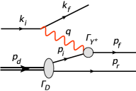
Figure 1: Exclusive electro-disinegration of the deuteron in plane wave impulse approximation:

Here, within PWIA the off-shellness of the bound nucleon is completely defined by the four-momentum of the deuteron, $p_{d}$ and spectator nucleon $p_{r}$: $p_{i}=p_{D}-p_{r}$. The one photon-exchange approximation allows to factorize electron and hadronic parts of the interaction in the invariant Feynman amplitude presented as follows:

$${\cal M}=\langle\lambda_{f}\mid j_{e}^{\nu}\mid\lambda_{i}\rangle{e^{2}g_{\nu\mu}\over q^{2}}\langle s_{f},s_{r}\mid A_{0}^{\mu}\mid s_{d}\rangle,$$ (2)

where $q^{2}$ is the virtual photon’s momentum squared. Here the leptonic current $j_{e}^{\nu}$ is defined as:

$$\langle\lambda_{f}\mid j_{e}^{\nu}\mid\lambda_{i}\rangle=\bar{u}(k_{f},\lambda_{f})\gamma^{\nu}u(k_{i},\lambda_{i}),$$ (3)

where $\langle s_{f},s_{r}\mid A_{0}^{\mu}\mid s_{d}\rangle$ represents the invariant amplitude of $\gamma^{*}d\rightarrow NN$ scattering,

Using Eq.(2) for the differential cross section of reaction (1) one obtains:

$${d\sigma\over d^{3}k_{f}/\epsilon_{f}d^{3}p_{f}/E_{f}}={1\over 4\sqrt{(p_{d}\cdot k_{i})^{2}}}{e^{4}\over q^{4}}L^{\mu\nu}H_{\mu\nu}{\delta((q+p_{d}-p_{f})^{2}-m_{N}^{2})\over 4(2\pi)^{5}}.$$ (4)

where, terms proportional to electron’s mass squared ($m_{e}^{2}$) are neglected. Here the leptonic tensor is defined as:

$$L^{\mu\nu}={1\over 2}\sum\limits_{\lambda_{1}\lambda_{2}}\left(\bar{u}(k_{f},\lambda_{f})\gamma^{\nu}u(k_{i},\lambda_{i})\right)^{\dagger}\bar{u}(k_{f},\lambda_{f})\gamma^{\mu}u(k_{i},\lambda_{i})$$ (5)

whereas the nuclear electromagnetic tensor is expressed through the scattering amplitude $A_{0}^{\mu}$ as follows:

$$H^{\mu\nu}={1\over 3}\sum\limits_{s_{d}s_{r}s_{f}}\langle s_{d}\mid A_{0}^{\mu\dagger}\mid s_{f},s_{r}\rangle\langle s_{f},s_{r}\mid A_{0}^{\nu}\mid s_{d}\rangle.$$ (6)

If one introduces $\Gamma_{\gamma^{*}}^{\mu}$ and $\Gamma_{D}$ invariant vertices (Fig.1) then within PWIA the amplitude $A_{0}^{\mu}$ can be presented in the form:

$$\langle s_{f},s_{r}\mid A_{0}^{\mu}\mid s_{d}\rangle=-\bar{u}(p_{f},s_{f})\Gamma_{\gamma^{*}}^{\mu}\frac{p\hskip-6.0pt/_{i}+m_{N}}{p_{i}^{2}-m^{2}_{N}}\cdot\bar{u}(p_{r},s_{r})\Gamma_{D}\cdot\chi^{s_{d}},$$ (7)

where $\chi^{s_{d}}$ is the spin wave function of the deuteron.

As it follows from the above equation $A_{0}^{\mu}$ contains neither the electron-bound nucleon scattering nor the nuclear wave function in the explicit form. The $eN_{bound}$ scattering and the nuclear wave function appears only when one considers the amplitude of Fig.1 in a time ordered perturbation theory in which case the invariant Feynman diagram splits into two time orderings as presented in Fig.2.

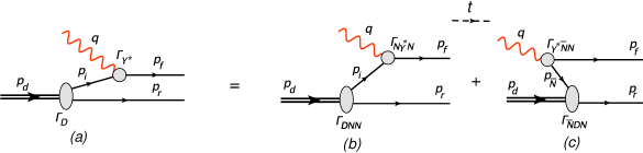
Figure 2: Representation of the covariant scattering amplitude (a) as a sum two time-ordered diagrams. (a) Virtual photon scattering from the bound nucleon; (b) Production of the $\bar{N}N$ pair by the virtual photon with subsequent absorption of the antinucleon by the deuteron.

Here, Fig.2(b) represents a scenario in which the virtual photon interacts with the preexisting bound nucleon in the deuteron with $\Gamma_{DNN}$ representing the vertex of $D\to NN$ transition and $\Gamma_{N\gamma^{*}N}$ the $\gamma^{*}N\rightarrow N$ electromagnetic interaction. Fig.2(c) however represents a very different scenario, in this case the virtual photon produces an intermediate $\bar{N}N$ state at the $\Gamma_{\gamma^{*}\bar{N}N}$ vertex with subsequent absorption of the antinucleon, $\bar{N}$ in the deuteron at the $\Gamma_{\bar{N}DN}$ vertex. The latter is not related to the $\gamma^{*}N$ scattering and the nucleon wave function in the deuteron. Fig.2(c) is commonly refereed as a ”Z-graph” and is a purely relativistic effect. As a result in the non-relativistic limit one deals with the diagram of Fig.2(b) only, which allows to express the covariant scattering amplitude through the nonrelativistic nuclear wave function and $\gamma^{*}N_{bound}$ scattering amplitude. However the situation becomes complicated when one is interested in the bound nucleon momentum $p_{i}\sim M_{N}$, which can be probed at momentum transfer $q\gg M_{N}$. In this case the ”Z-graph” contribution (Fig.2(c)) becomes comparable with the one in Fig.2(b) preventing the straightforward introduction of the nuclear wave function.

This situation is reminiscent to the QCD processes in probing partonic structure of hadrons in which case due to the relativistic nature of partons, vacuum diagrams can not be neglected in the time ordered perturbation theory defined in the lab frame of the hadronFeynman . The solution in this case is to consider the scattering process in the infinite momentum frame (or on the light-front), which allows to suppress the ”Z-graphs” and consider only the diagrams similar to Fig.2 (b) for which one can introduce the wave function of the constituents.

Our approach in probing deeply bound nucleon is similar to that of the partonic model, in which we consider the reaction (1) on the light-front allowing us to exclude the contribution of the vacuum diagrams (Fig.2(c)) and introduce a light-front nuclear wave function.

III Derivation within Effective Light-Front Perturbation Theory

III.1 Scattering amplitude in PWIA

We consider now the reaction (1) on the light-front, where the light-cone time is defined as $\tau\equiv t+z$. To calculate the PWIA amplitude of the reaction (1) we apply effective light-front perturbation theory (LFPT) in the $\tau$-time ordered representation of the scattering amplitude $A_{0}^{\mu}$. In such approach the scattering amplitude (7) is expressed as a sum of the noncovariant diagrams presented in Fig.3. Here in addition to the two $\tau$ orderings analogous to the time ordering of Fig.2 one has an additional contribution of Fig.3(c) corresponding to the instantaneous interaction due to the spinor nature of the bound nucleon.

To proceed with the calculations we choose a reference frame with $z$ axis antiparallel to the transferred momentum, $\hat{z}\ ||\ -{\bf q}$, such that the deuteron is aligned along $\hat{z}$.

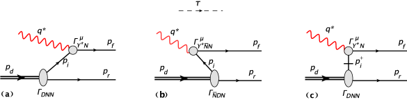
Figure 3: Representation of the covariant scattering amplitude as a sum of two light-cone ($\tau$)-time -ordered diagrams as well as instantaneous interaction. (a) Virtual photon scattering from the bound nucleon; (b) Production of the $\bar{N}N$ pair by the virtual photon with subsequent absorption of the antinucleon by the deuteron., (c) Instantaneous interaction of virtual photon with the bound nucleon.

The calculations are performed in the Light-Cone (LC) reference frame in which case where the four-momenta are defined as $(p^{+},p^{-},p_{x},p_{y})$, where $p^{\pm}=E\pm p_{z}$ with $p^{+}$ representing the light-cone longitudinal momentum. We employ the $\gamma$-matrix algebra using the following light-cone definitions:

$$\gamma^{\mu}=(\gamma^{+},\gamma^{-},\gamma_{1},\gamma_{2}),\ \ \ \mbox{where}\ \ \ \gamma^{\pm}=\gamma_{0}\pm\gamma_{3}.$$ (8)

The scalar products and other properties of four-vectors as well as $\gamma$ matrices on the light-front are given in Appendix A.

We also define the light-cone momentum fractions, which are Lorentz invariant quantities with respect to boosts along the $z$ direction:

$$\alpha_{r}={2p_{r}^{+}\over p_{d}^{+}},\ \ \ \alpha_{q}={2q^{+}\over p_{d}^{+}},\ \ \ \alpha_{f}={2p_{f}^{+}\over p_{d}^{+}},\ \ \ \alpha_{N}=\alpha_{f}-\alpha_{q}=2-\alpha_{r}.$$ (9)

Here $\alpha_{r}$, $\alpha_{q}$ and $\alpha_{f}$ correspond to the fraction of LC ”+” component of the deuteron momentum carried by the recoil nucleon, virtual photon and final knock-out nucleon respectively. The light-cone momentum fraction of the bound nucleon $\alpha_{N}$ is defined through the energy-momentum conservation.

We proceed with the calculation of the scattering amplitude corresponding to the diagrams of Fig.3 by applying the Light-Front perturbation rules (KS(1970) ; LB(1980) ) in an effective theory in which one identifies effective vertices for nuclear transition and electron-bound nucleon scattering (see Appendix A). At each vertices the transverse, $p_{\perp}$ and plus, $p^{+}$ components of momenta are conserved. Because of the latter and the chosen reference frame in which $q^{+}=q_{0}-|\textbf{q}|<0$ the diagram of the Fig.3(b) will not contribute since the production of $\bar{N}N$ pair will require $q^{+}>0$. The remaining diagrams represent the amplitudes in which the virtual photon knocks-out a bound nucleon which propagates from the $d\rightarrow NN$ transition vertex to the $\gamma^{*}N$ interaction point, $A^{\mu}_{prop}$ (Fig.3(a)), and the instantaneous amplitude, $A^{\mu}_{inst}$ (Fig.3(c)) in which $d\rightarrow NN$ transition and $\gamma^{*}N$ interaction take place at the same light cone time -$\tau$. In both diagrams the nucleus exposes its constituents and the scattering takes place off the bound nucleon, which allow us to introduce the light-front nuclear wave function and the amplitude of $\gamma^{*}N_{bound}$ scattering.

We now apply the light-front diagrammatic rulesLB(1980) (summarized in Appendix A) which yields for the propagating part of the scattering amplitude (Fig.3(a)):

$$\langle s_{f},s_{r}\mid A_{prop}^{\mu}\mid s_{d}\rangle=-\bar{u}(p_{f},s_{f})\Gamma_{\gamma^{*}N}^{\mu}\ \frac{1}{p_{i}^{+}}\frac{(p\hskip-6.0pt/_{i}+m_{N})_{on}}{(p_{d}^{-}-p_{r}^{-}-p_{i,on}^{-})}\bar{u}(p_{r},s_{r})\Gamma_{DNN}\chi^{s_{d}},$$ (10)

where $p_{d}^{-}$, $p_{r}^{-}$ and $p_{i,on}^{-}$ are defined from the on-energy shell condition: $p^{-}={m_{j}^{2}+p_{\perp,j}^{2}\over p_{j}^{+}}$ with $j=d,r,(i,on)$. The ”on” subscript in $(p\hskip-6.0pt/_{i}+m_{N})_{on}$ indicates that all the components of the bound nucleon light-cone momenta are taken on-energy shell.

For the instantaneous diagram of Fig.3(c) applying the rules of Appendix A one obtains:

$$\langle s_{f},s_{r}\mid A_{inst}^{\mu}\mid s_{d}\rangle=-\bar{u}(p_{f},s_{f})\Gamma_{\gamma^{*}N}^{\mu}\frac{1}{p_{i}^{+}}\left(\frac{1}{2}\gamma^{+}\right)\bar{u}(p_{r},s_{r})\Gamma_{DNN}\chi^{s_{d}}.$$ (11)

Note that in both expressions (10) and (11) one has the same nuclear, $\Gamma_{DNN}$ and electromagnetic, $\Gamma_{\gamma^{*}N}$ vertices.

For further elaborations, we introduce the off-energy shell ”-” component of the bound nucleon $p_{i}^{-}=p_{d}^{-}-p_{r}^{-}$ , and using the definition: $p_{j}^{-}={m_{j}^{2}+p_{j,\perp^{2}}\over p_{j}^{+}}$ for the on-energy-shell ”-” component for $j=d,r$ as well as Eq.(9) one obtains:

$$\frac{1}{p_{d}^{-}-p^{-}_{r}-p^{-}_{i,on}}=\frac{1}{p_{i}^{-}-p^{-}_{i,on}}=\frac{p_{d}^{+}}{M_{d}^{2}-4\frac{(m_{N}^{2}+p_{\bot}^{2})}{\alpha(2-\alpha)}}.$$ (12)

Using the above relation as well as the sum rule relation for on-shell spinors:

$$(p\hskip-6.0pt/_{i}+m_{N})_{on}=\sum_{s_{i}}\left(u(p_{i},s_{i})\bar{u}(p_{i},s_{i})\right)_{on},$$ (13)

for the sum of the two amplitudes in Eqs.(10) and (11) one obtains:

$$A^{\mu}=A^{\mu}_{prop}+A^{\mu}_{inst}= -\bar{u}(p_{f},s_{f})\Gamma_{\gamma^{*}N}^{\mu}\frac{\sum_{s_{i}}u(p_{i},s_{i})\bar{u}(p_{i},s_{i})}{\frac{\alpha}{2}\left(M^{2}_{d}-4\frac{m^{2}_{N}+{\bf p_{T}}^{2}}{\alpha\left(2-\alpha\right)}\right)}\bar{u}(p_{r},s_{r})\Gamma_{DNN}\chi^{s_{d}}$$ (15)

$$-\bar{u}(p_{f},s_{f})\Gamma_{\gamma^{*}N}^{\mu}\frac{\frac{1}{2}\gamma^{+}\left({p}_{i}^{-}-{p}_{i,on}^{-}\right)}{\frac{\alpha}{2}\left(M^{2}_{d}-4\frac{m^{2}_{N}+{\bf p_{T}}^{2}}{\alpha\left(2-\alpha\right)}\right)}\bar{u}(p_{r},s_{r})\Gamma_{DNN}\chi^{s_{d}}.$$

Within PWIA we can factorize the above expression in the form of a product of electromagnetic current and the light-front nuclear wave function. For this we introduce the light-front wave functions in the formFS81 ; Artiles_Sargsian-multisrc1 :

$$\psi^{s_{i}s_{r}s_{d}}_{LF}\left(\alpha,{\bf p_{T}}\right)=-\frac{\bar{u}(p_{i},s_{i})\bar{u}(p_{r},s_{r})\Gamma_{DNN}\chi^{s_{d}}}{\frac{1}{2}\left(M^{2}_{d}-4\frac{m^{2}_{N}+{\bf p_{T}}^{2}}{\alpha\left(2-\alpha\right)}\right)}\dfrac{1}{\sqrt{2\left(2\pi\right)^{3}}}.$$ (16)

From the above definition one also obtains:

$$\frac{1}{\frac{\alpha}{2}\left(M^{2}_{d}-4\frac{m^{2}_{N}+{\bf p_{T}}^{2}}{\alpha\left(2-\alpha\right)}\right)}\bar{u}(p_{r},s_{r})\Gamma_{DNN}\ \chi^{s_{d}}=-\sum_{s_{i}}\frac{u(p_{i},s_{i})}{2m_{N}}\frac{\psi^{s_{i}s_{r}s_{d}}_{LF}\left(\alpha,{\bf p_{T}}\right)}{\alpha}\sqrt{2\left(2\pi\right)^{3}}$$ (17)

Using now the above Eqs.(16) and (17) in $A_{prop}^{\mu}$ and $A_{inst}^{\mu}$ respectively, the Eq.(15) can be presented in the form:

$$A^{\mu}=A^{\mu}_{prop}+A^{\mu}_{inst}=\sum_{s_{i}}J^{\mu}_{N}\left(p_{f}s_{f},p_{i}s_{i}\right)\dfrac{\psi^{s_{i}s_{r}s_{d}}_{LF}\left(\alpha,{\bf p_{T}}\right)}{\alpha}\sqrt{2\left(2\pi\right)^{3}},$$ (18)

where we introduced the electromagnetic current of the bound nucleon as follows:

$$J^{\mu}_{N}(p_{f}s_{f},p_{i}s_{i})=\bar{u}(p_{f}s_{f})\Gamma_{\gamma\ast N}^{\mu}u(p_{i}s_{i})+\bar{u}(p_{f}s_{f})\Gamma_{\gamma\ast N}^{\mu}\frac{\gamma^{+}\left({p}_{i}^{-}-{p}_{i\ on}^{-}\right)}{4m_{N}}u(p_{i}s_{i}).$$ (19)

Here, the Dirac spinor of the initial nucleon $u(p_{i},s_{i})$ is defined for the on-shell momentum, $p_{i,on}=(p^{-}_{i,on},p_{i}^{+},p_{i}^{\perp})$. Our main focus in the following sections will be the electromagnetic current of Eq.(19, which characterizes the interaction of the electron probe with the bound nucleon.

III.2 Propagating and Instantaneous Components of Electromagnetic Current

To identify the propagating and instantaneous parts of the electromagnetic current in Eq.(19) we consider first the electromagnetic vertex $\Gamma_{\gamma\ast N}^{\mu}$. Since the final state of the interacting nucleon is on mass shell, and only the positive light-front energy projections enter in the amplitude, we are led to the half off-shell vertex function in the general form (see e.g. Bincer60 ; Koch90 ; Koch96 :

$$\Gamma_{\gamma^{\ast}N}^{\mu}=\gamma^{\mu}F_{1}+i\sigma^{\mu\nu}q_{\nu}F_{2}{\kappa\over 2m_{N}}+q^{\mu}F_{3},$$ (20)

where the form-factors $F_{1,2,3}=F_{1,2,3}(m_{N}^{2},p_{i}^{2},q^{2})$ are functions of Lorentz invariants constructed from the momenta of initial and final nucleons and momentum transfer $q$. In general one expects $F_{1,2}(m_{N}^{2},p_{i}^{2},q^{2})$ not to be identical with the corresponding on-shell nucleon form-factors ($F_{1,2}(m_{N}^{2},m_{N}^{2},q^{2})$). This difference is due to the modification of the internal structure of nucleons in the nuclear medium. Such modification, in principle, should originate from the dynamics similar to the one responsible for the medium modification of partonic distributions of bound nucleon - commonly referred as EMC effect (EMC ). This however is out of the scope of our discussion since we are interested only in the effects related to the off-shellness of the interacting nucleon’s electromagnetic current. Thus, in the numerical estimates we will use unmodified nucleon form-factors measured for free nucleons. Concerning to $F_{3}$, it does not contribute to the cross section of the process due to the gauge invariance of the leptonic current: $q_{\mu}j_{e}^{\mu}=0$. However for consistency one can estimate the $F_{3}$ form-factor based on the fact that due to the conservation of the momentum sum rule in light-front approach the electromagnetic current of the bound-nucleon is conserved:

$$q_{\mu}J_{N}^{\mu}=0.$$ (21)

Using Eq.(19) together with (20) one obtains: $F_{3}=F_{1}{q\hskip-4.0pt/\over Q^{2}}$. Inserting the later into Eq.(20) one can separate the propagating and instantaneous parts of the electromagnetic vertex in the form

$$\Gamma_{\gamma^{\ast}N}^{(prop)\mu}=\gamma^{\mu}F_{1}+i\sigma^{\mu\nu}q_{\nu}F_{2}{\kappa\over 2m_{N}},$$ (22)

and

$$\Gamma_{\gamma^{\ast}N}^{(inst)\mu}=\left(\gamma^{\mu}F_{1}+i\sigma^{\mu\nu}q_{\nu}F_{2}{\kappa\over 2m_{N}}\right)\frac{\Delta p\hskip-6.0pt/_{i}}{2m_{N}}-F_{1}{q^{\mu}\over q^{2}}q\hskip-6.0pt/\Big{(}{\bf 1}+\frac{\Delta p\hskip-6.0pt/_{i}}{2m_{N}}\Big{)},$$ (23)

where, $\Delta{p}_{i}^{\mu}=p^{\mu}_{i}-p^{\mu}_{i,on}$ and $2\Delta p\hskip-6.0pt/_{i}=\gamma^{+}\left(p^{-}_{i}-p^{-}_{i,on}\right)$ since $\Delta p_{i}^{+}=\Delta p_{i}^{\perp}=0$. In the following derivations we will use the relation:

$$\Delta{p}_{i}^{-}=-q^{-}+(p_{f}^{-}-p_{i,on}^{-})=\dfrac{Q^{2}}{q^{+}}-\dfrac{m^{2}_{N}+{\bf p_{T}}^{2}}{p_{f}^{+}p_{i}^{+}}q^{+}=\frac{1}{p_{d}^{+}}\left(M_{d}^{2}-4\frac{(m_{N}^{2}+{\bf p_{T}}^{2})}{\alpha(2-\alpha)}\right),$$ (24)

as well as:

$$2\Delta{p}_{i}\cdot p_{i}=\Delta{p}_{i}^{-}p_{i}^{+}=p_{i}^{2}-m_{N}^{2},$$ (25)

which allow to express the electromagnetic current in boost-invariant variables.

The separation of the electromagnetic vertex into propagating and instantaneous parts in Eqs.(22) and (23 allows to separate the electromagnetic current in Eq.(19) into corresponding parts in the following form:

$$J_{N}^{\mu}(p_{f}s_{f},p_{i}s_{i})=J^{\mu}_{prop}(p_{f}s_{f},p_{i}s_{i})+J^{\mu}_{inst}(p_{f}s_{f},p_{i}s_{i})$$ (26)

where,

$$J^{\mu}_{prop}(p_{f}s_{f},p_{i}s_{i}) = \bar{u}(p_{f}s_{f})\Gamma_{\gamma\ast N}^{(prop)\mu}u(p_{i}s_{i})$$

$$J^{\mu}_{inst}(p_{f}s_{f},p_{i}s_{i}) = \bar{u}(p_{f}s_{f})\Gamma_{\gamma\ast N}^{(inst)\mu}u(p_{i}s_{i}).$$ (27)

It is worth mentioning that even though the propagating vertex in Eq.(22) has the same form as the free on-shell nucleon vertex the corresponding electromagnetic current $J^{\mu}_{prop}$ does not correspond to an on-shell scattering amplitude, since $q^{\mu}\neq p_{f}^{\mu}-p_{i,on}^{\mu}$. Also, the current conservation (Eq.(21)) is satisfied only for the sum of the propagating and instantaneous currents in Eq.(26).

III.3 Off-Shell Parameter of $eN_{bound}$ Scattering

While the off-shell effects in the propagating vertex of Eq.(22) are kinematical, due to the fact that $q^{\mu}\neq p_{f}^{\mu}-p_{i,on}^{\mu}$, the off-shell effects in the instantaneous vertex are dynamical. The latter interaction arises exclusively due to the binding of the nucleon. As it follows from Eq.(23) the strength of the instantaneous vertex is proportional to the magnitude of the factor $\Delta p_{i}^{-}$ defined in Eq.(24). One can express the $\Delta p_{i}^{-}$ factor through a boost invariant quantities by defining the light-front reference frame such that the four-momenta of the deuteron, $p_{d}^{\mu}$ and momentum transfer $q^{\mu}$ are:

$$p_{d}^{\mu} = ({Q^{2}\over m_{N}},{m_{d}^{2}m_{N}\over Q^{2}},\bf{0_{T}})$$ (28)

$$q^{\mu} = (-{Q^{2}x\over m_{N}(1+\sqrt{1+{4m_{N}^{2}x^{2}\over Q^{2}}}\ )},{m_{N}\over x}(1+\sqrt{1+{4m_{N}^{2}x^{2}\over Q^{2}}}),\bf{0_{T}}).$$

Using above definitions one introduces the off-shell parameter $\eta$ such that,

$$\Delta{p}_{i}^{-}=-{m_{N}}\eta,$$ (29)

where,

$$\eta={1\over Q^{2}}\left(4\frac{(m_{N}^{2}+{\bf p_{T}}^{2})}{\alpha(2-\alpha)}-m_{d}^{2}\right).$$ (30)

As it will be shown in the derivations bellow, the parameter $\eta$ provides the universal measure of the off-shell effect which combines both the resolution of the probe through the $Q^{2}$ and the binding effects of the nucleon through the light-cone variables, $\alpha$ and $\bf{p_{T}}$.

IV Electron-Nucleon Scattering Cross Section

In many practical applications one needs to evaluate the electron-bound-nucleon cross section $\sigma_{eN}$ as it is defined in Ref.deForest(1983) . Such a cross section is calculated within PWIA in which case using Eq.(18) the nuclear electromagnetic tensor of Eq.(6) can be expressed as follows:

$$H^{\mu\nu}=H^{\mu\nu}_{N}(p_{f},p_{i})\ \rho_{d}\left(\alpha,{\bf p_{T}}\right)\ \dfrac{2-\alpha}{\alpha^{2}}\ 2\left(2\pi\right)^{3},$$ (31)

where spin averaged light cone density matrix of the deuteron $\rho_{d}(\alpha,p_{T})$ and bound nucleon electromagnetic tensor $H^{\mu\nu}_{N}(p_{f},p_{i})$ are defined in the following forms:

$$\rho\left(\alpha,{\bf p_{T}}\right)=\dfrac{1}{2s_{d}+1}\cdot\frac{1}{2}\sum_{s_{d},s_{i},s_{r}}\dfrac{\left|\psi^{s_{i}s_{r}s_{d}}_{LF}\left(\alpha,{\bf p_{T}}\right)\right|^{2}}{2-\alpha}$$ (32)

and

$$H^{\mu\nu}_{N}=\frac{1}{2}\sum_{s_{i}s_{f}=-1/2}^{1/2}J_{N}^{\nu}\left(p_{f}s_{f},p_{i}s_{i}\right)^{\dagger}J^{\mu}_{N}\left(p_{f}s_{f},p_{i}s_{i}\right).$$ (33)

Inserting now Eq.(31) into Eq.(4) the Lorentz invariant cross section of the reaction (1) can be presented as follows:

$${d\sigma\over d^{3}k_{f}/\epsilon_{f}d^{3}p_{f}/E_{f}}={1\over 2p_{d}\cdot k_{i}}{\alpha^{2}_{EM}\over q^{4}}L_{\mu\nu}H^{\mu\nu}_{N}\rho\left(\alpha,{\bf p_{T}}\right)\dfrac{2-\alpha}{\alpha^{2}}\delta\left(p_{r}^{2}-m_{N}^{2}\right),$$ (34)

where $\alpha_{EM}=e^{2}/(4\pi)$. Introducing the light-front nuclear spectral function in the form:

$$S_{d}^{LF}(\alpha,{\bf p_{T}})=\rho_{d}\left(\alpha,{\bf p_{T}}\right)\dfrac{2-\alpha}{\alpha^{2}}\delta\left(p_{r}^{2}-m_{N}^{2}\right),$$ (35)

similar to Ref.(deForest(1983) ) one can present the differential cross section as a product of $\sigma_{eN}$ and the spectral function as follows:

$${d\sigma\over d\epsilon_{f}d\Omega_{k_{f}}d^{3}p_{f}}=\sigma_{eN}\ S_{d}^{LF}(\alpha,{\bf p_{T}}),$$ (36)

were

$$\sigma_{eN}={1\over 2m_{D}\epsilon_{i}}\ {\epsilon_{f}\over E_{f}}\ {\alpha^{2}_{EM}\over q^{4}}\ L_{\mu\nu}H^{\mu\nu}_{N}.$$ (37)

Here $\epsilon_{i}$, $\epsilon_{f}$ are initial and scattered electron energies. The $E_{f}$ represents the energy of the knock-out nucleon.

It is worth mentioning that the expression in Eq.(36) is universal for any nuclei in which case one needs to replace the deuteron spectral function by the light-front spectral function of the nucleus being considered.

IV.1 Structure Functions of Bound Nucleon

In calculating $\sigma_{eN}$ in Eq.(37) it is convenient to present it through the four independent structure functions of the nucleon $V^{N}_{L}$, $V^{N}_{TL}$, $V^{N}_{T}$ and $V^{N}_{TT}$ in the form:

$$\sigma_{eN}={1\over 2m_{D}E_{f}}\ {\sigma_{Mott}}\left(\eta_{L}V_{L}^{N}+\eta_{TL}V_{TL}^{N}\cos\phi+\eta_{T}V_{T}^{N}+\eta_{TT}V_{TT}^{N}\cos(2\phi)\right),$$ (38)

where $\sigma_{Mott}={\alpha^{2}\cos({\theta\over 2})^{2}\over 4\epsilon_{i}^{2}\sin({\theta\over 2})^{4}}$ with $\theta$ being scattered electron angle. In the above equation:

$$\eta_{L} = \frac{Q^{4}}{{\bf q}^{4}}$$

$$\eta_{T} = \frac{Q^{2}}{2{\bf q}^{2}}+\tan^{2}\frac{\theta}{2}$$

$$\eta_{TT} = \frac{Q^{2}}{2{\bf q}^{2}}$$

$$\eta_{TL} = \frac{Q^{2}}{{\bf q}^{2}}\left(\frac{Q^{2}}{{\bf q}^{2}}+\tan^{2}\frac{\theta}{2}\right)^{1/2},$$ (39)

where $Q^{2}=4\epsilon_{i}\epsilon_{f}\sin({\theta\over 2})^{2}$, and $\bf q$ is the three momentum of the virtual photon. The above defined structure functions of the bound nucleon can be related to the light-front components of the nucleonic electromagnet tensor as follows (see Appendix B):

$$V^{N}_{L} = \frac{{\bf q}^{2}}{4Q^{2}}\left(H^{++}{Q^{2}\over(q^{+})^{2}}+2H^{+-}+{(q^{+})^{2}\over Q^{2}}H^{--}\right)$$

$$V^{N}_{TL} = {|{\bf q}|\over q^{+}}\left(H^{+\parallel}_{N}+H^{-\parallel}_{N}{(q^{+})^{2}\over Q^{2}}\right)$$

$$V^{N}_{T} = H^{\parallel\parallel}_{N}+H^{\bot\bot}_{N}$$

$$V^{N}_{TT} = H_{N}^{\parallel\parallel}-H_{N}^{\bot\bot}$$ (40)

where $\pm$ correspond to $t\pm\hat{z}$ directions on the light-cone with $\hat{z}$ defined in the negative direction of of the transfered three momentum $\bf q$. The transverse components are chosen as follows: the perpendicular direction is defined by $\textbf{n}_{\bot}=\frac{\textbf{p}_{f}\times\textbf{q}}{|\textbf{p}_{f}\times\textbf{q}|}$, and the parallel unit vector projection is $\textbf{n}_{\parallel}=\frac{\textbf{q}\times\textbf{n}_{\bot}}{|\textbf{q}\times\textbf{n}_{\bot}|}$. The scattering and reaction planes of the reaction are defined in Fig.4.

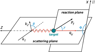
Figure 4: Definition of scattering and reaction planes of knock-out reaction.

Using now the Eq.(33) and the expression of the bound nucleon electromagnetic current from Eqs.(26), and (27) one can calculate nucleon structure functions explicitly. In what follows we split the structure functions into two terms:

$$V^{N}_{i}=V^{N}_{i,prop}+V^{N}_{i,inst}\ \ \ \ \text{for i = L,TL,T,TT}$$ (41)

where subscript ”prop” corresponds to the structure functions calculated using the propagating part of the electromagnetic current, $J_{prop}^{\mu}$ only, while the terms with the subscript ”inst” correspond to the contribution from $J_{inst}^{\mu}$ and its interference with $J_{prop}^{\mu}$.

Using the explicit forms of the currents from Eqs.(26),(27) we calculate the above structure functions expressing them through the off-shell parameter $\eta$ (Eq.(30)) as follows:

$$V_{L\ prop}^{N} = {\bf{q}}^{2}\left[F_{1}^{2}\tau^{-1}\left(1+{p^{2}_{\textbf{T}}\over m_{N}^{2}}+\tau\eta_{i}(\eta_{i}+\eta_{q})\right)-F_{1}F_{2}{\kappa}\left(2+\eta_{q}\right)+F_{2}^{2}\kappa^{2}\left({p^{2}_{\textbf{T}}\over m_{N}^{2}}+\tau(1+\eta_{q})\right)\right],$$

$$\vspace*{0.3cm}V_{L\ inst}^{N} = {\bf{q}}^{2}\Big{[}F_{1}^{2}\eta_{i}\Big{(}\tau\eta_{i}(1+\eta_{q})-2-\eta_{q}\Big{)}+F_{1}F_{2}\kappa\Big{(}\tau\eta_{i}\left(2-2\eta_{i}-\eta_{q}\right)+\eta_{q}\Big{)}$$

$$+F_{2}^{2}\kappa^{2}\tau\Big{(}\tau\eta_{i}(\eta_{i}+\eta_{q})-\eta_{q}\Big{)}\Big{]},$$

$$\vspace*{0.3cm}V_{TL\ prop}^{N} = 2\ |{\bf{q}}|\ p_{\textbf{T}}\left(F_{1}^{2}+F_{2}^{2}\kappa^{2}\tau\right)\left[2+4{\alpha_{N}\over\alpha_{q}}+2\eta_{i}+\eta_{q}\right],$$

$$\vspace*{0.3cm}V_{TL\ inst}^{N} = 2|{\bf{q}}|p_{\textbf{T}}\left(F_{1}^{2}+F_{2}^{2}\kappa^{2}\tau\right)\left(1-\tau\eta_{i}\right)\eta_{q},$$

$$\vspace*{0.3cm}V_{T\ prop\ \ }^{N} = \ 4m_{N}^{2}\left[F_{1}^{2}\left({p^{2}_{\textbf{T}}\over m_{N}^{2}}+2\tau(1+\eta_{q})\right)+2F_{1}F_{2}{\kappa}\tau\left(2+\eta_{q}\right)+F_{2}^{2}\kappa^{2}\tau\left(2+{p^{2}_{\textbf{T}}\over m_{N}^{2}}+2\tau\eta_{i}(\eta_{i}+\eta_{q})\right)\right],$$

$$\vspace*{0.3cm}V_{T\ inst\ \ }^{N} = 2Q^{2}\Big{[}F_{1}^{2}\Big{(}\tau\eta_{i}(\eta_{i}+\eta_{q})-\eta_{q}\Big{)}+F_{1}F_{2}\kappa\Big{(}\tau\eta_{i}\left(2\eta_{i}+\eta_{q}-2\right)-\eta_{q}\Big{)}$$

$$+F_{2}^{2}\kappa^{2}\tau\eta_{i}\Big{(}\tau\eta_{i}(1+\eta_{q})-2-\eta_{q}\Big{)}\Big{]},$$

$$\vspace*{0.3cm}V_{TT\ prop}^{N} = 4p_{\textbf{T}}^{2}\left(F_{1}^{2}+F_{2}^{2}\kappa^{2}\tau\right),$$

$$\vspace*{0.3cm}V_{TT\ inst}^{N} = 0,$$ (42)

where, $\tau=Q^{2}/(4m_{N}^{2})$, $\ \eta_{i}=\eta\ \alpha_{N}/2$, $\ \eta_{q}=\eta\ \alpha_{q}/2$. Alternatively, one can write,

$$\eta_{i} = -{2\Delta{p}_{i}\cdot p_{i}\over Q^{2}}={(m^{2}_{N}+{\bf p_{T}}^{2})\over Q^{2}}\dfrac{\alpha_{q}}{\alpha_{f}}-\dfrac{\alpha_{N}}{\alpha_{q}},$$ (43)

$$\eta_{q} = -{2\Delta{p}_{i}\cdot q\over Q^{2}}={(m^{2}_{N}+{\bf p_{T}}^{2})\over Q^{2}}\dfrac{\alpha_{q}^{2}}{\alpha_{f}\alpha_{N}}-1.$$ (44)

The structure functions in Eq.(42) are Lorentz invariant and expressed through the boost invariant variables $\eta$, $\alpha_{i}$, $\alpha_{q}$ and $\alpha_{f}$. Since many experiments in probing high momentum bound nucleons are performed in the fixed target experiments it is convenient to express the above variables through the four momenta measured in the lab frame. Considering a Lab reference frame in which $\hat{z}||{\bf q}$, the $\alpha_{i}$, $\alpha_{q}$ and $\alpha_{f}$ parameters can be expressed as follows:

$$\alpha_{i}=2-\alpha_{r}=\alpha_{f}-\alpha_{q},\ \ \ \alpha_{r}={2(E_{r}-p_{r}cos\theta_{r})\over m_{d}},\ \ \ \alpha_{q}={2(q_{0}-{\bf q})\over m_{d}},\ \ \ \alpha_{f}={2(E_{f}-p_{f}cos\theta_{f})\over m_{d}},$$ (45)

where, $p_{d}^{\mu}=(m_{d},0)$, $q^{\mu}=(q_{0},{\bf q})$, $p_{r}^{\mu}=(E_{r},{\bf p_{r}})$ and $p_{f}^{\mu}=(E_{f},{\bf p_{f}})$ are four-momenta of the target deuteron, virtual photon, recoil and struck nucleon measured in the Lab frame.

V Numerical Estimates

We present numerical estimates for kinematics which will be explored in experiments planned for 12 GeV upgraded Jefferson Lab. In all calculations below we take the initial energy of the electron beam $\epsilon_{i}=11$ GeV.

To quantify the extent of the binding effects we consider the ratio:

$$R={\sigma_{eN}\over\sigma_{eN}^{on}},$$ (46)

where $\sigma_{eN}$ is the cross section of electron bound nucleon scattering defined in Eq.(37) for given initial momenta $\bf{p_{i}}$ or ($\alpha_{i}$ and $p_{T}$), while $\sigma_{eN}^{on}$ corresponds to the same cross section for the electron scattering off the free moving nucleon with the same initial momenta.

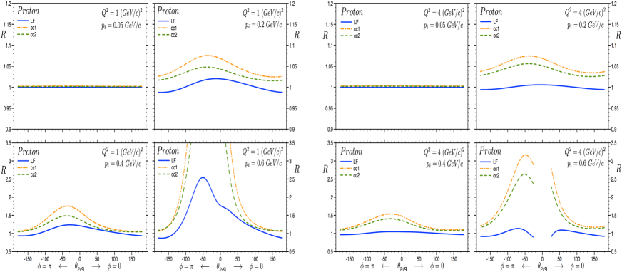
Figure 5: The $\theta_{p_{i}q}$ dependence of ratios of the off-shell cross section of electron-bound proton scattering to that of the one-shell cross section. The solid lines are LF approximation, dashed and dash-dotted curves corresponds to CC2 and CC1 versions of de Forest approximationdeForest(1983) . The panels correspond to the bound nucleon momenta $p_{i}=50,200,400$ and $600$ MeV/c for $Q^{2}=1$ and $4$ (GeV/c)². The minus sign of $\theta_{pq}$ indicates on kinematics corresponding to $\phi=180^{0}$ between scattering and reaction planes. Calculations done for initial electron energy $\epsilon_{i}=11$ GeV.

First, we consider the dependence of $R$ on ”traditional” kinematical parameters which define the electronuclear processes such as initial momentum of the bound nucleon ($p_{i}$) its relative angle with respect to the transferred 3-momentum ($\bf q$) as well as the virtuality of the transferred momentum ($Q^{2}$). Additionally we compare the predictions of LF approximation with that of the de Forest formalismdeForest(1983) which is commonly used in the analysis of the experimental data. In all these estimates we use the same parameterization for the electric and magnetic form-factors of the nucleons. These parameterizations are the same for the free nucleon. Thus we do not consider the effects related to the possible modification of the charge and magnetic current distributions in the bound nucleon.

In Fig.5 and Fig.6 we compare the angular dependences of ratio $R$ at different values of missing momenta at fixed $Q^{2}=1$ and $4$ (GeV/c)² for bound proton and neutron respectively. As Fig.5 shows LF approximation predicts off-shell effects for $Q^{2}=1$ (GeV/c)² as large as $40-250\%$ for bound proton momenta $\geq 400$ MeV/c. Even larger effects are expected within the de Forest approachdeForest(1983) . We observe also that the prediction within LF and de Forest approximations significantly diverge close to the kinematical limit of the scattering process as it can be seen in calculations for $p_{i}=600$ MeV/c.

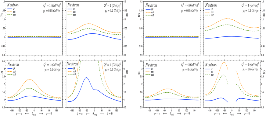
Figure 6: The same as in Fig.5 but for scattering from bound neutron.

Because of different magnitudes and signs of form-factors one predicts somewhat different off-shell effects for scattering from a bound proton or neutron. However, qualitatively the dependences of $R$ for kinematical parameters of the reaction for both proton and neutron are similar.

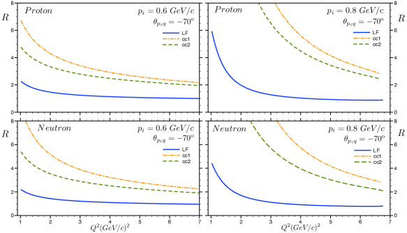
Figure 7: The $Q^{2}$ dependence of the off-shell effects for $\theta_{p_{i}q}=-70^{0}$ for proton and neutron targets.

An important feature of LF calculations following from Fig.5 and Fig.6 is the diminishing of the off-shell effects with an increase of $Q^{2}$. This reflects the dynamical nature of the LF approximation in which case the harder the probe (larger $Q^{2}$) lesser is the sensitivity to the binding effects of the target nucleon. It is worth mentioning that no such behavior exists in the de Forest approximation since in this case part of the off-shell effects are kinematical in which the energy of bound nucleon is taken to be equal to the on-shell energy for the given momentum of the nucleon, with the phase space of the initial nucleon being proportional to ${1\over\sqrt{m_{N}^{2}+p_{i}^{2}}}$.

To ascertain the extent of the $Q^{2}$ suppression on the off-shell effects, in Fig.7 we present the $Q^{2}$ dependence of the ratio $R$ for proton and neutron initial momenta of $p_{i}=600$  and $800$ MeV/c. Here we choose $\theta_{p_{i}q}=-70^{0}$ for which large off-shell effects are observed in Fig.5 and Fig.6. These calculations indicate that already at $Q^{2}\geq 4$ GeV² the off-shell effects predicted in light-front approximation are not more than $10\%$ for such a large bound nucleon momenta.

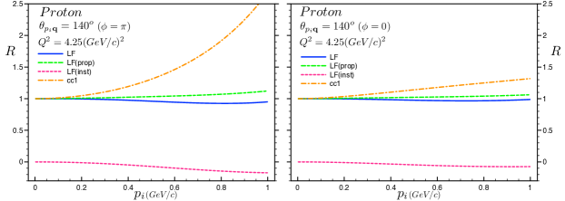
Figure 8: Off shell effects expected for the experiment of Ref.Boeglin:2014aca (left panel). The right-panel is the similar effects for $\phi=0$ kinematics.

For practical purposes in Fig.8 we estimate the dependence of the off-shell effects on the momentum of the bound nucleon for kinematics relevant to the planned JLAB experimentBoeglin:2014aca which is aimed at probing deuteron structure at very large internal momenta. As the figure shows for both cases of the angles between scattering and reaction planes ($\phi$) the light-front approach predicts off-shell effects to be less than $8\%$ for all kinematics with the latter value happening at $p_{i}=850$ MeV/c.

At the end of the section we discuss whether the parameter $\eta$ introduced in Eq.(30) can be used as a universal parameter for estimation of the of-shell effects for any kinematic conditions of electro-production reaction. For this, in Fig. 9 we calculate the $\eta$ dependence of $|R-1|$ for very large magnitudes of bound nucleon momenta ($p_{i}=600$ and $800$ MeV/c) at different values of transverse momentum $p_{T}$. Note that, the expected off-shell effects will be much less for smaller values of $p_{i}$.

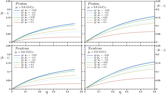
Figure 9: The $\eta$ parameter dependence of the off-shell effects $|R-1|$ for $p_{i}=0.6$ and $0.8$ GeV/c at different values of the transverse momentum $p_{T}$.

As the figure shows for any possible scenarios of kinematics the off shell effects can be confined below $5\%$ as soon as $\eta<0.1$. This represents a strong indication that the variable $\eta$ can be considered as an universal parameter for controlling the off-shell effects in the reaction mechanism of electron-nuclear processes.

VI Summary and Outlook

Based on light-front approach we calculated electron-deuteron scattering within PWIA which allowed us to isolate the electron-bound-nucleon scattering cross section, $\sigma_{eN}$. Within LF approximation the vacuum contribution naturally disappears while the off-shell nature of the nucleon results in a appearance of an instantaneous term in the electromagnetic current of electron-bound nucleon scattering. In deriving $\sigma_{eN}$ we separated the propagating and instantaneous contributions in the electromagnetic current which allowed explicitly to trace the effects associated with the binding of the nucleon.

Furthermore in LF approach we were able to identify the parameter (defined as $\eta$) that universally characterizes the extent of the off-shellness of electromagnetic current.

The derived $\sigma_{eN}$ is used to estimate the expected off-shell effects in electro-nuclear processes in kinematics relevant to the 12 GeV energy upgraded Jefferson Lab experiments. We compared the LF predictions with that of the de Forest approximation widely used by experimentalists to estimate the off-shell effects in the reaction mechanism of electro-nuclear processes. These comparisons indicate that practically in all kinematic cases the LF approach predicts less off-shell effects at $Q^{2}\geq 1$ GeV² than the de Forest approximation does. Most importantly the LF approach predicts a significant drop of the off-shell effects with an increase of $Q^{2}$ which intuitively can be understood as a decrease in the sensitivity of the hard processes on the off-shellness of the target nucleon.

We also checked our conjecture that the $\eta$-variable can be considered as a universal parameter in controlling off-shell effects. We found that for wide range of kinematics the off-shell effects can be suppressed on the level of $5\%$ as as soon as $\eta<0.1$. The latter gives an effective method for controlling the uncertainties in the reaction mechanism for large varieties of electro-nuclear processes probing deeply bound nucleons in the nucleus.

Finally, it is worth mentioning that even though we considered the $eA$ scattering within PWIA the obtained expressions for electromagnetic current are applicable also for scattering amplitudes in which the final state interaction between outgoing nucleons is considered within eikonal approximation. In this case (see e.g. Refs.gea ; ms01 ) the main part of the re-scattering amplitude is evaluated at the pole value of the struck nucleon propagator in the intermediate state. As a result the entered electromagnetic current is again half-off-shell as the considered electromagnetic current in Eq.(26).

Appendix A Light Front Perturbation Theory Rules

We present here a summary of the rules for computation of amplitudes within Light Front (LF) formalism.

The LF scalar product and notations are (Lepage-Brodsky conventionLB(1980) ; BPP(1997) ):

$$\ x\cdot p={1\over 2}\left(x^{+}p^{-}+x^{-}p^{+}\right)-\textbf{x}_{\textbf{T}}\cdot\textbf{p}_{\textbf{T}}$$

$$x^{\mu}=\left(x^{+},{x}^{-},x,y\right)=\left(x^{+},{x}^{-},\textbf{x}_{\textbf{T}}\right)\ ,\ p^{\mu}=\left(p^{+},p^{-},\textbf{p}_{\textbf{T}}\right)$$

$$x^{\pm}=t\pm z$$ (47)

Figure 10: Example of the scattering amplitude on the light-front ($\tau=x^{+}$ flows from left to right).

Diagrammatic Rules for effective light-front perturbation theory can be formulated as follows:

1. Draw all topologically distinct $\tau\equiv x^{+}$-ordered diagrams at the desired coupling power. In addition to the usual advanced and retarded propagation between two events one needs to include a third possibility in which the two events connected by an internal fermion or photon interact at the same LF $\tau$- time, commonly referred as instantaneous term.

2. Assign to each line a four-momentum $p^{\mu}$ and spin $s$ (or helicity, $\lambda$) corresponding to a single on-mass-shell particle, i.e. $p^{2}=m^{2}$.

3. With spin 1/2 fermions associate on-mass-shell spinors $u(p,s)$, with antifermions $v(p,s)$, with photons $\epsilon_{\mu}(q,\lambda)$, etc, such that,

   $$\bar{u}(p,s^{\prime})u(p,s) = -\bar{v}(p,s^{\prime})v(p,s)=2m\delta_{ss^{\prime}}$$

   $$\sum_{s}u(p,s)\bar{u}(p,s) = p\hskip-6.0pt/+m$$

   $$\sum_{s}v(p,s)\bar{v}(p,s) = p\hskip-6.0pt/-m$$

   $$\epsilon^{\mu}(q,\lambda^{\prime})\epsilon^{\mu}(q,\lambda) = -\delta_{\lambda^{\prime}\lambda}\ ,\ \ q\cdot\epsilon(q,\lambda)=0$$

   $$\sum_{\lambda}\epsilon^{\mu}(q,\lambda)\epsilon^{\nu}(q,\lambda) = -g^{\mu\nu}+{q^{\mu}\eta^{\nu}+q^{\nu}\eta^{\mu}\over q\cdot\eta}$$ (48)

   where $\eta$ is a null vector ($\eta^{2}=0$), given in LC gauge by, $\eta=(0,2,0,0)$

4. Each intermediate state gets a factor (inverse of the difference of the sums over initial and intermediate LF energies ($p_{-}$):

   $$\frac{1}{\sum_{ini}p^{-}-\sum_{int}p^{-}+i\epsilon}$$ (49)

   where, ’$ini$’ stands for the initial state of the diagram and ’$int$’ for intermediate states. All particles are on-mass-shell, that is: $\ p^{-}=\frac{m^{2}+p_{\textbf{T}}^{2}}{p_{i}^{+}}>0$.

5. Internal lines account for two kind of interactions:

   • Propagating, in which case, for a vertex like in Fig.(10)(a) one has:

     $$\Gamma\ \bar{u}(p^{\prime},s^{\prime})\epsilon\hskip-6.0pt/(q,\lambda)u(p,s)\delta^{2}(\sum_{in}p_{\textbf{T}}-\sum_{out}p_{\textbf{T}})\delta(\sum_{in}p^{+}-\sum_{out}p^{+})$$ (50)

     where, ’$in$’ and ’$out$’ mean flowing into and out of the vertex. The $\delta$ functions at the vertex provide an explicit conservation of the plus and transverse components of ’$in$’ and ’$out$’ momenta.

   • Instantaneous. For each vertex like in Fig.(10)(b) (fermionic), include,

     $$\Gamma^{2}\ \bar{u}(p^{\prime},s^{\prime})\epsilon\hskip-6.0pt/(q^{\prime},\lambda^{\prime}){\gamma^{+}\over 2(q^{+}-p^{\prime+})}\epsilon\hskip-6.0pt/(q,\lambda)u(p,s)\delta^{2}(\sum_{in}p_{\textbf{T}}-\sum_{out}p_{\textbf{T}})\delta(\sum_{in}p^{+}-\sum_{out}p^{+}).$$ (51)

     And, for each vertex like in Fig.(10) (c) (vector), include,

     $$\Gamma^{2}\ \bar{u}(p^{\prime},s^{\prime})\gamma^{+}u(p,s){1\over(p^{\prime+}-p^{+})^{2}}\bar{u}(k^{\prime},\sigma^{\prime})\gamma^{+}u(k,\sigma)\delta^{2}(\sum_{in}p_{\textbf{T}}-\sum_{out}p_{\textbf{T}})\delta(\sum_{in}p^{+}-\sum_{out}p^{+}).$$ (52)

   Here $\Gamma$ factors represent effective vertices which can be specified for the particular case of the scattering. They can correspond to electron-bound nucleon scattering as well as nuclear transition to the constituent nucleons. The conditions for for which such an effective vertices can be introduced in the Feynman diagrams are discussed in Ref.ms01 .

6. Sum over polarizations and integrate over each internal line with the factor,

   $$\sum_{s}\int\frac{dp_{\textbf{T}}dp^{+}}{2(2\pi)^{3}p^{+}}\Theta(p^{+})$$

   which ensures the plus component positivity (all particles move forward in LC time.)

7. Include symmetry factors. Also, a factor of -1 for each fermion loop, for fermion lines beginning and ending at the initial state, and for each diagram in which fermion lines are interchanged in either of the initial or final states, as well as the overall sign from Wick’s theorem.

Appendix B Nucleonic Tensor

Substituting Eq.(26) into Eq.(33), allows us to express the nucleonic tensor as a sum of two terms:

$$H^{\mu\nu}_{N}=H^{\mu\nu}_{N\ prop}+H^{\mu\nu}_{N\ inst},$$ (53)

where the the propagating contribution is given by,

$$H^{\mu\nu}_{N\ prop}={1\over 2}\sum_{s_{i}s_{f}}(J^{s_{i}s_{f}\ \mu}_{prop})^{\dagger}(J^{s_{i}s_{f}}_{prop})^{\nu}=\frac{1}{2}Tr\left[\overline{\Gamma}_{\gamma^{\ast}N}^{(on)\mu}(p\hskip-6.0pt/_{f}+m_{N})\Gamma_{\gamma^{\ast}N}^{(on)\nu}(p\hskip-6.0pt/_{i,on}+m_{N})\right],$$ (54)

and the instantaneous by,

$$H^{\mu\nu}_{N\ inst} = {1\over 2}\sum_{s_{i}s_{f}}\left((J^{s_{i}s_{f}\ \nu}_{off})^{\dagger}J^{s_{i}s_{f}\ \mu}_{inst}+(J^{s_{i}s_{f}\ \nu}_{prop})^{\dagger}J^{s_{i}s_{f}\ \mu}_{inst}+(J^{s_{i}s_{f}\ \nu}_{inst})^{\dagger}J^{s_{i}s_{f}\ \mu}_{prop}\right)$$

$$= \dfrac{1}{2}Tr\Big{[}\overline{\Gamma}_{\gamma^{\ast}N}^{(off)\nu}(p\hskip-6.0pt/_{f}+m_{N})\Gamma_{\gamma^{\ast}N}^{(off)\mu}(p\hskip-6.0pt/_{i,on}+m_{N})$$

$$+\overline{\Gamma}_{\gamma^{\ast}N}^{(on)\nu}(p\hskip-6.0pt/_{f}+m_{N})\Gamma_{\gamma^{\ast}N}^{(off)\mu}(p\hskip-6.0pt/_{i,on}+m_{N})+\overline{\Gamma}_{\gamma^{\ast}N}^{(off)\nu}(p\hskip-6.0pt/_{f}+m_{N})\Gamma_{\gamma^{\ast}N}^{(on)\mu}(p\hskip-6.0pt/_{i,on}+m_{N})\Big{]},$$

where, $\overline{\Gamma}_{\gamma^{\ast}N}^{\mu}=\gamma^{0}\left({\Gamma}_{\gamma^{\ast}N}^{\mu}\right)^{\dagger}\gamma^{0}$. Notice that the initial momentum of the nucleon, $p_{i}$, occurring from now-on corresponds to $p_{i,on}$, which allows to drop the on-shell label ”on” without confusion. With this, we can write propagating and instantaneous contributions of the tensor, $H^{\mu,\nu}$ as functions of the nucleon form factors $F_{1}$ and $F_{2}$ as follows:

$$H^{\mu\nu}_{N\ prop} = \ 2F_{1}^{2}\Big{[}g^{\mu\nu}\left(m_{N}^{2}-p_{i}\cdot p_{f}\right)+\left(p_{i}^{\mu}p_{f}^{\nu}+p_{i}^{\nu}p_{f}^{\mu}\right)\Big{]}$$ (56)

$$+ F_{1}F_{2}\kappa\Big{[}2g^{\mu\nu}q\cdot\left(p_{f}-p_{i}\right)+\left(p_{i}^{\mu}q^{\nu}+p_{i}^{\nu}q^{\mu}\right)-(p_{f}^{\mu}q^{\nu}+p_{f}^{\nu}q^{\mu})\Big{]}$$

$$+ F_{2}^{2}{\kappa^{2}\over 2m_{N}^{2}}\Big{[}g^{\mu\nu}\big{[}q^{2}\left(p_{i}\cdot p_{f}+m_{N}^{2}\right)-2\ q\cdot p_{i}\ q\cdot p_{f}\big{]}-q^{2}\left(p_{i}^{\mu}p_{f}^{\nu}+p_{i}^{\nu}p_{f}^{\mu}\right)$$

$$\ \ \ \ -q^{\mu}q^{\nu}\left(p_{i}\cdot p_{f}+m_{N}^{2}\right)+q\cdot p_{f}\left(p_{i}^{\mu}q^{\nu}+p_{i}^{\nu}q^{\mu}\right)+q\cdot p_{i}\left(p_{f}^{\mu}q^{\nu}+p_{f}^{\nu}q^{\mu}\right),\Big{]}$$

and the instantaneous correction as follows:

$$H^{\mu\nu}_{N\ inst}=\ 2F_{1}^{2}\Big{[}g^{\mu\nu}\Big{(}\Delta p_{i}\cdot\left(p_{i}-p_{f}\right)-{\Delta p_{i}\cdot p_{i}\over m_{N}^{2}}\Delta p_{i}\cdot p_{f}\Big{)}+\left(\Delta p_{i}^{\mu}p_{f}^{\nu}+\Delta p_{i}^{\nu}p_{f}^{\mu}\right)\Big{(}1+{\Delta p_{i}\cdot p_{i}\over m_{N}^{2}}\Big{)}$$ (57)

$$+ {2\over q^{2}}q^{\mu}q^{\nu}\Big{(}{2\over q^{2}}q\cdot p_{f}\ q\cdot(\Delta p_{i}+p_{i})-(p_{i}-p_{f})\cdot(\Delta p_{i}+p_{i})+{\Delta p_{i}\cdot p_{i}\over m_{N}^{2}}\Big{(}{\Delta p_{i}\cdot q\over q^{2}}p_{f}\cdot q+{\Delta p_{i}\cdot p_{f}}\Big{)}\Big{)}$$

$$- {2\over q^{2}}\left(p_{i}^{\mu}q^{\nu}+p_{i}^{\nu}q^{\mu}\right)q\cdot p_{f}-{2\over q^{2}}(p_{f}^{\mu}q^{\nu}+p_{f}^{\nu}q^{\mu})\Big{(}q\cdot(\Delta p_{i}+p_{i})+{\Delta p_{i}\cdot p_{i}\over m_{N}^{2}}\Delta p_{i}\cdot q\Big{)}$$

$$- {2\over q^{2}}\left(\Delta p_{i}^{\mu}q^{\nu}+\Delta p_{i}^{\nu}q^{\mu}\right)q\cdot p_{f}\Big{(}1+{\Delta p_{i}\cdot p_{i}\over m_{N}^{2}}\Big{)}\Big{]}$$

$$+ F_{1}F_{2}\kappa\Big{[}g^{\mu\nu}\Big{(}{\Delta p_{i}\cdot p_{i}\over m_{N}^{2}}q\cdot(2p_{f}-\Delta p_{i})-2\Delta p_{i}\cdot q\Big{)}+q^{\mu}q^{\nu}\Big{(}{\Delta p_{i}\cdot p_{i}\over m_{N}^{2}q^{2}}q\cdot(\Delta p_{i}-2p_{f})-2\Big{)}$$

$$\ \ \ \ \ \ \ \ -\left(p_{i}^{\mu}q^{\nu}+p_{i}^{\nu}q^{\mu}\right)+(p_{f}^{\mu}q^{\nu}+p_{f}^{\nu}q^{\mu})\Big{]}$$

$$+ F_{2}^{2}{\kappa^{2}\over 2m_{N}^{2}}\Big{[}g^{\mu\nu}\big{[}\left(q^{2}\ \Delta p_{i}\cdot p_{f}-2\ q\cdot\Delta p_{i}\ q\cdot p_{f}\right)\Big{(}1+{\Delta p_{i}\cdot p_{i}\over m_{N}^{2}}\Big{)}+q^{2}\ \Delta p_{i}\cdot p_{i}\big{]}$$

$$\ \ \ \ \ \ \ -\left(\Delta p_{i}^{\mu}p_{f}^{\nu}+\Delta p_{i}^{\nu}p_{f}^{\mu}\right)q^{2}\Big{(}1+{\Delta p_{i}\cdot p_{i}\over m_{N}^{2}}\Big{)}-q^{\mu}q^{\nu}\big{[}\Delta p_{i}\cdot p_{f}\Big{(}1+{\Delta p_{i}\cdot p_{i}\over m_{N}^{2}}\Big{)}-\Delta p_{i}\cdot p_{i}\big{]}$$

$$\ \ \ \ \ \ \ +\left(\Delta p_{i}^{\mu}q^{\nu}+\Delta p_{i}^{\nu}q^{\mu}\right)q\cdot p_{f}\Big{(}1+{\Delta p_{i}\cdot p_{i}\over m_{N}^{2}}\Big{)}+\left(p_{f}^{\mu}q^{\nu}+p_{f}^{\nu}q^{\mu}\right)q\cdot\Delta p_{i}\Big{(}1+{\Delta p_{i}\cdot p_{i}\over m_{N}^{2}}\Big{)}\Big{]}.$$

With our choice of reference frame (Fig.(4)), one can expand the $L_{\mu\nu}H^{\mu\nu}$ product in the following form:

$$L_{\mu\nu}H^{\mu\nu}_{N} = \left(L_{00}H^{00}-2L_{0z}H^{0z}+L_{zz}H^{zz}\right)+\left(-2L_{0\parallel}H^{0\parallel}+2L_{z\parallel}H^{z\parallel}\right)$$ (58)

$$+ \frac{1}{2}\left(L_{\parallel\parallel}+L_{\bot\bot}\right)\left(H^{\parallel\parallel}+H^{\bot\bot}\right)+{1\over 2}\left(L_{\parallel\parallel}-L_{\bot\bot}\right)\left(H^{\parallel\parallel}-H^{\bot\bot}\right).$$

Furthermore, using the gauge-invariance of leptonic current, one expresses the above product in the form:

$$L_{\mu\nu}H^{\mu\nu}_{N} = L_{00}\left(H^{00}-2{q^{0}\over q_{z}}H^{0z}+\left({q^{0}\over q_{z}}\right)^{2}H^{zz}\right)+2L_{0\parallel}\left(-H^{0\parallel}+{q^{0}\over q_{z}}H^{z\parallel}\right)$$ (59)

$$+ \frac{1}{2}\left(L_{\parallel\parallel}+L_{\bot\bot}\right)\left(H^{\parallel\parallel}+H^{\bot\bot}\right)+{1\over 2}\left(L_{\parallel\parallel}-L_{\bot\bot}\right)\left(H^{\parallel\parallel}-H^{\bot\bot}\right)$$

$$= Q^{2}(\tan(\theta/2))^{2}\left(\eta_{L}V_{N,L}+\eta_{TL}V_{N,TL}\cos(\phi)+\eta_{T}V_{N,T}+\eta_{TT}V_{N,TT}\right).$$

Using the definitions of $\eta_{i}$ for $i=L,T,TL,TT$, from Eq.(30) for hadronic structure functions, ($V_{N,i}$), one obtains:

$$V^{N}_{L} = \frac{{\bf q}^{4}}{Q^{4}}\left(H^{00}-2{q^{0}\over q_{z}}H^{0z}+({q^{0})^{2}\over{\bf q}^{2}}H^{zz}\right)=\frac{{\bf q}^{2}}{4Q^{2}}\left(H^{++}{Q^{2}\over(q^{+})^{2}}+2H^{+-}+{(q^{+})^{2}\over Q^{2}}H^{--}\right)$$

$$V^{N}_{TL} = 2{{\bf q}^{2}\over Q^{2}}\left({q^{0}\over q_{z}}H^{z\parallel}_{N}-H^{0\parallel}_{N}\right)={|{\bf q}|\over q^{+}}\left(H^{+\parallel}_{N}+H^{-\parallel}_{N}{(q^{+})^{2}\over Q^{2}}\right)$$

$$V^{N}_{T} = H^{\parallel\parallel}_{N}+H^{\bot\bot}_{N}$$ (60)

$$V^{N}_{TT} = H_{N}^{\parallel\parallel}-H_{N}^{\bot\bot},$$ (61)

where we have used, $-q_{z}=|{\bf q}|$, as well as the relation between components of the nucleonic tensor in light-cone and Minkowski coordinates:

$$H^{00} = {1\over 4}(H^{++}+2H^{+-}+H^{--})$$

$$H^{0z} = {1\over 4}(H^{++}-H^{--})$$

$$H^{zz} = {1\over 4}(H^{++}-2H^{+-}+H^{--})$$

$$H^{0\parallel} = {1\over 2}(H^{+\parallel}+H^{-\parallel})$$

$$H^{z\parallel} = {1\over 2}(H^{+\parallel}-H^{-\parallel}).$$ (62)

From Eqs.(56, B) we compute the explicit forms of the structure functions. In the reference frame of Fig.(4), they are given by:

$$V_{L\ prop}^{N} = F_{1}^{2}{\bf{q}}^{2}\dfrac{\alpha_{N}\alpha_{f}}{\alpha_{q}^{2}}\Big{(}{m^{2}_{N}+p_{\textbf{T}}^{2}\over Q^{2}}\dfrac{\alpha_{q}^{2}}{\alpha_{N}\alpha_{f}}+1\Big{)}-F_{1}F_{2}{\bf{q}}^{2}{\kappa}\left({m^{2}_{N}+p_{\textbf{T}}^{2}\over Q^{2}}\dfrac{\alpha_{q}^{2}}{\alpha_{N}\alpha_{f}}+1\right)$$

$$+F_{2}^{2}{\bf{q}}^{2}\left({\kappa\over 2m_{N}}\right)^{2}\left((m^{2}_{N}+p_{\textbf{T}}^{2})\dfrac{\alpha_{q}^{2}}{\alpha_{N}\alpha_{f}}+4p_{\textbf{T}}^{2}\right)$$

$$V_{L\ inst}^{N} = F_{1}^{2}{\alpha_{N}\over\alpha_{q}}{\bf{q}}^{2}\left(1-\left({m^{2}_{N}+p_{\textbf{T}}^{2}\over Q^{2}}\dfrac{\alpha_{q}^{2}}{\alpha_{N}\alpha_{f}}\right)^{2}+{(m^{2}_{N}+p_{\textbf{T}}^{2})\over 2m^{2}}\dfrac{\alpha_{q}}{\alpha_{N}}+\left({m^{2}_{N}+p_{\textbf{T}}^{2}\over Q^{2}}\dfrac{\alpha_{q}^{2}}{\alpha_{N}\alpha_{f}}-1\right)^{2}\right)$$

$$-2F_{1}F_{2}\kappa{\alpha_{N}\over\alpha_{q}}{\bf{q}}^{2}{(q\cdot\Delta p_{i})^{2}\over m^{2}Q^{2}}\left(2{\alpha_{f}\over\alpha_{q}}+2{m^{2}\over q\cdot\Delta p_{i}}+1\right)$$

$$+F_{2}^{2}\Big{(}{\kappa\over m^{2}_{N}}\Big{)}^{2}{\bf{q}}^{2}~{}q\cdot\Delta p_{i}\left(1+{q\cdot\Delta p_{i}\over m^{2}}{\alpha_{N}\alpha_{f}\over\alpha_{q}^{2}}\right)$$

$$V_{TL\ prop}^{N} = |{\bf{q}}|\dfrac{\alpha_{N}+\alpha_{f}}{\alpha_{q}}p_{\textbf{T}}\left(2F_{1}^{2}+2F_{2}^{2}\Big{(}{\kappa\over 2m_{N}}\Big{)}^{2}Q^{2}\right)\left(1+{m^{2}_{N}+p_{\textbf{T}}^{2}\over Q^{2}}\dfrac{\alpha_{q}^{2}}{\alpha_{N}\alpha_{f}}\right)$$

$$V_{TL\ inst}^{N} = 8|{\bf{q}}|{q\cdot\Delta p_{i}\over Q^{2}}p_{\textbf{T}}\left(1+{p_{i}\cdot\Delta p_{i}\over m^{2}}\right)\left(F_{1}^{2}+F_{2}^{2}\Big{(}{\kappa\over 2m_{N}}\Big{)}^{2}\right)$$

$$V_{T\ prop\ \ }^{N} = \ F_{1}^{2}\left(2(m^{2}_{N}+p_{\textbf{T}}^{2})\dfrac{\alpha_{q}^{2}}{\alpha_{N}\alpha_{f}}+4(p_{\textbf{T}})^{2}\right)+2\kappa F_{1}F_{2}\left((m^{2}_{N}+p_{\textbf{T}}^{2})\dfrac{\alpha_{q}^{2}}{\alpha_{N}\alpha_{f}}+Q^{2}\right)$$

$$+F_{2}^{2}\left({\kappa\over 2m_{N}}\right)^{2}\left(2\dfrac{\alpha_{N}\alpha_{f}}{\alpha_{q}^{2}}\left((m^{2}_{N}+p_{\textbf{T}}^{2})\dfrac{\alpha_{q}^{2}}{\alpha_{N}\alpha_{f}}+Q^{2}\right)^{2}-4Q^{2}p_{\textbf{T}}^{2}\right)$$

$$V_{T\ inst\ \ }^{N} = 8F_{1}^{2}\left(q\cdot\Delta p_{i}+p_{f}\cdot\Delta p_{i}{p_{i}\cdot\Delta p_{i}\over m^{2}}\right)+8F_{1}F_{2}\kappa\left(1+{p_{i}\cdot\Delta p_{i}\over m^{2}}\right)\left(q\cdot\Delta p_{i}-p_{f}\cdot q{p_{i}\cdot\Delta p_{i}\over m^{2}+p_{i}\cdot\Delta p_{i}}\right)$$

$$+8F_{2}^{2}\left({\kappa\over 2m_{N}}\right)^{2}\left(1+{p_{i}\cdot\Delta p_{i}\over m^{2}}\right)\left(q\cdot p_{f}~{}q\cdot\Delta p_{i}+Q^{2}~{}p_{f}\cdot\Delta p_{i}+Q^{2}{m^{2}~{}p_{i}\cdot\Delta p_{i}\over m^{2}+p_{i}\cdot\Delta p_{i}}\right)$$

$$V_{TT\ prop}^{N} = 4p_{\textbf{T}}^{2}\left(F_{1}^{2}+F_{2}^{2}{\kappa^{2}\over 4m_{N}^{2}}Q^{2}\right)$$

$$V_{TT\ off}^{N} = 0.$$ (63)

The kinematic variables, and scalar products used in the calculation are as follows:

The light-cone momentum fractions are:

$$\alpha_{N}={2p_{N}^{+}\over p_{d}^{+}}={2(E_{N}+p_{N,z})\over p_{d}^{+}},\ \ \ \alpha_{q}={2q^{+}\over p_{d}^{+}}={2(q^{0}-|{\bf{q}}|)\over p_{d}^{+}},\ \ \ \alpha_{f}=\alpha_{N}+\alpha_{q}$$ (64)

and the off-shell factor is, $\Delta{p}_{i}^{\mu}=p^{\mu}_{i}-p^{\mu}_{i,on}$, with, $p^{\mu}_{i}=p^{\mu}_{d}-p^{\mu}_{r}$. Since $\Delta p_{i}^{+}=\Delta p_{i}^{\perp}=0$, we have, $2\Delta p\hskip-6.0pt/_{i}=\gamma^{+}\left(p^{-}_{i}-p^{-}_{i,on}\right)$ with the minus component defined as follows:

$$\Delta{p}_{i}^{-}=p_{i}^{-}-p_{i\ on}^{-}=-q^{-}+(p_{f}^{-}-p_{i\ on}^{-})=\dfrac{Q^{2}}{q^{+}}-\dfrac{m^{2}_{N}+p_{\bot}^{2}}{p_{f}^{+}p_{i}^{+}}q^{+}.$$ (65)

The scalar products of initial ($p_{i,on}^{\mu}$), final ($p_{f}^{\mu}$) and transferred ($q^{\mu}$) momenta with the off-shell factor $\Delta{p}_{i}^{\mu}$, can be written as:

$$2\Delta{p}_{i}\cdot p_{i} = Q^{2}\dfrac{\alpha_{N}}{\alpha_{q}}-(m^{2}_{N}+{\bf p_{T}}^{2})\dfrac{\alpha_{q}}{\alpha_{f}}$$

$$2\Delta{p}_{i}\cdot p_{f} = Q^{2}\dfrac{\alpha_{f}}{\alpha_{q}}-(m^{2}_{N}+{\bf p_{T}}^{2})\dfrac{\alpha_{q}}{\alpha_{i}}$$

$$2\Delta{p}_{i}\cdot q = Q^{2}-(m^{2}_{N}+{\bf p_{T}}^{2})\dfrac{\alpha_{q}^{2}}{\alpha_{f}\alpha_{N}}.$$ (66)

References

- (1) N. Fomin, D. Higinbotham, M. Sargsian and P. Solvignon, Ann. Rev. Nucl. Part. Sci. 67, 129 (2017).
- (2) O. Hen, G. A. Miller, E. Piasetzky and L. B. Weinstein, Rev. Mod. Phys. 89, no. 4, 045002 (2017).
- (3) W. Boeglin and M. Sargsian, Int. J. Mod. Phys. E 24, no. 03, 1530003 (2015).
- (4) C. Ciofi degli Atti, Phys. Rept. 590, 1 (2015).
- (5) J. Arrington, D. W. Higinbotham, G. Rosner and M. Sargsian, Prog. Part. Nucl. Phys. 67, 898 (2012).
- (6) L. Frankfurt, M. Sargsian and M. Strikman, Int. J. Mod. Phys. A 23, 2991 (2008).
- (7) L. L. Frankfurt, M. I. Strikman, D. B. Day and M. Sargsian, Phys. Rev. C 48, 2451 (1993).
- (8) K. S. Egiyan et al. [CLAS Collaboration], Phys. Rev. C 68, 014313 (2003).
- (9) K. S. Egiyan et al. [CLAS Collaboration], Phys. Rev. Lett. 96, 082501 (2006).
- (10) N. Fomin et al., Phys. Rev. Lett. 108, 092502 (2012).
- (11) A. Tang et al., Phys. Rev. Lett. 90, 042301 (2003).
- (12) R. Shneor et al. [Jefferson Lab Hall A Collaboration], Phys. Rev. Lett. 99, 072501 (2007).
- (13) E. Piasetzky, M. Sargsian, L. Frankfurt, M. Strikman and J. W. Watson, Phys. Rev. Lett. 97, 162504 (2006).
- (14) R. Subedi et al., Science 320, 1476 (2008).
- (15) M. M. Sargsian, Phys. Rev. C 89, no. 3, 034305 (2014).
- (16) O. Hen et al., Science 346, 614 (2014).
- (17) O. Artiles and M. M. Sargsian, Phys. Rev. C94, 064318.
- (18) L. L. Frankfurt, M. M. Sargsian and M. I. Strikman, Phys. Rev. C 56, 1124 (1997).
- (19) M. M. Sargsian, Int. J. Mod. Phys. E 10, 405 (2001).
- (20) C. Ciofi degli Atti and L. P. Kaptari, Phys. Rev. C 71, 024005 (2005).
- (21) S. Jeschonnek and J. W. Van Orden, Phys. Rev. C 78, 014007 (2008).
- (22) J. M. Laget, Phys. Lett. B 609, 49 (2005).
- (23) M. M. Sargsian, T. V. Abrahamyan, M. I. Strikman and L. L. Frankfurt, Phys. Rev. C 71, 044614 (2005).
- (24) M. M. Sargsian, T. V. Abrahamyan, M. I. Strikman and L. L. Frankfurt, Phys. Rev. C 71, 044615 (2005).
- (25) M. M. Sargsian, Phys. Rev. C 82, 014612 (2010).
- (26) W. Cosyn and M. Sargsian, Phys. Rev. C 84, 014601 (2011).
- (27) W. Cosyn and M. Sargsian, Int. J. Mod. Phys. E 26, no. 09, 1730004 (2017).
- (28) A. Bussiere et al., Nucl. Phys. A 365, 349 (1981).
- (29) S. Turck-Chieze et al., Phys. Lett. 142B, 145 (1984).
- (30) J. F. J. Van Den Brand et al., Phys. Rev. Lett. 60, 2006 (1988).
- (31) S. Frullani and J. Mougey, Adv. Nucl. Phys. 14, 1 (1984).
- (32) T. de Forest, Nuclear Physics A392 232-248 (1983)
- (33) R. P. Feynman, “Photon-hadron interactions,” Reading 1972, 282p.
- (34) J. Kogut and D. Soper, Phys. Rev. D1, 2901 (1970).
- (35) G. P. Lepage and S. J. Brodsky, Phys. Rev. D 22, 2157 (1980).
- (36) L. L. Frankfurt and M. I. Strikman, Phys. Rept. 76, 215 (1981).
- (37) S. J. Brodsky, H. C. Pauli and S. S. Pinsky, Phys. Rept. 301, 299 (1998).
- (38) L. L. Frankfurt and M. I. Strikman, Nucl. Phys. B 148, 107 (1979).
- (39) B. D. Keister and W. N. Polyzou. Adv. Nucl. Phys. 20, 225 (1991).
- (40) G. A. Miller, Prog. Part. Nucl. Phys. 45, 83 (2000).
- (41) W. W. Buck and F. Gross, Phys. Rev. D 20, 2361 (1979).
- (42) S. D. Glazek, Acta Phys. Polon. B 14, 893 (1983).
- (43) G. A. Miller, Phys. Rev. C 89, no. 4, 045203 (2014).
- (44) A. M. Bincer, Phys. Rev. 118, 855 (1960).
- (45) H. W. L. Naus, S. J. Pollock, J. H. Koch and U. Oelfke, Nucl. Phys. A509 717-735 (1990)
- (46) H. W. L. Naus, S. J. Pollock, J. H. Koch, Phys. Rev. C53, 2304 (1996)
- (47) J. J. Aubert et al. [European Muon Collaboration], Phys. Lett. 123B, 275 (1983).
- (48) W. U. Boeglin et al., arXiv:1410.6770 [nucl-ex].