Agnostic tests can control the type I and type II errors simultaneously

Abstract

Despite its common practice, statistical hypothesis testing presents challenges in interpretation. For instance, in the standard frequentist framework there is no control of the type II error. As a result, the non-rejection of the null hypothesis $(H_{0})$ cannot reasonably be interpreted as its acceptance. We propose that this dilemma can be overcome by using agnostic hypothesis tests, since they can control the type I and II errors simultaneously. In order to make this idea operational, we show how to obtain agnostic hypothesis in typical models. For instance, we show how to build (unbiased) uniformly most powerful agnostic tests and how to obtain agnostic tests from standard p-values. Also, we present conditions such that the above tests can be made logically coherent. Finally, we present examples of consistent agnostic hypothesis tests.

1 Introduction

Despite its common practice, statistical hypothesis testing presents challenges in interpretation. For instance, some understand that an hypothesis test can either accept or reject the null hypothesis, $H_{0}$. However, in this paradigm the probability of accepting $H_{0}$ can be high even when $H_{0}$ is false. Therefore, it is possible to obtain the undesirable result of accepting $H_{0}$ even when this hypothesis is unlikely.

In order to deal with this problem, others propose that an hypothesis test should either reject or fail to reject $H_{0}$ (Casella and Berger 3, p. 374 and DeGroot and Schervish 5, p. 545). Such a position can also lead to challenges in interpretation, since the practitioner often wishes to be able to assert $H_{0}$ [13]. For example, in regression analysis non-significant predictors are often considered to not affect the response variable and are removed from the model. More generally, scientists often wish to assert a theory [20, 21].

Neyman [17][p.14] briefly introduces an alternative to the above paradigms to hypothesis testing. In this setting, an hypothesis test can have three outcomes: reject $H_{0}$, accept $H_{0}$, or remain in doubt about $H_{0}$ — the agnostic decision. This third decision allows the hypothesis test to commit a less severe error (remain in doubt) whenever the data doesn’t provide strong evidence either in favor or against the null hypothesis. This approach, which was called agnostic hypothesis testing, was further developed in Berg [1], Esteves et al. [6], Stern et al. [22]. This framework allows the acceptance of $H_{0}$ while simultaneously controlling the type I and II errors through the agnostic decision. As a result, it is possible to control the probability that $H_{0}$ is accepted when $H_{0}$ is false.

Although agnostic decisions have been used in classification problems with great success [12, 9, 10, 18] the agnostic hypothesis testing framework has only started to be explored. Here, we generalize to arbitrary hypotheses the setting in Berg [1], which applies only to hypotheses of the form: $H_{i}:\theta=\theta_{i}$, for $i\in\{0,1\}$. This generalization allows the translation of standard concepts, such as level, size, power, p-value, unbiased tests, and uniformly most powerful test into the framework of agnostic hypothesis testing. Within this framework, we create new versions of standard statistical techniques, such as t-tests, regression analysis and analysis of variance, which simultaneously control type I and type II errors.

Section 2 formally defines agnostic tests and concepts that are used for controlling their error, such as level, size and power. Sections 2.1 and 2.2 use these definitions to generalize the framework in Berg [1]; they derive agnostic tests that are uniformly most powerful tests and unbiased uniformly most powerful tests. Since it can be hard to obtain the above tests in complex models, Section 3 derives a general approach for controlling the error of agnostic tests that is based on p-values. Section 4 advances results that were obtained in Esteves et al. [6], Stern et al. [22] and shows that agnostic tests can control type I and II errors while retaining logical coherence. Section 5 discusses how to control the type I and II errors while obtaining consistent agnostic tests. All proofs are presented in the supplementary material.

2 The power of agnostic tests

We consider a setting in which the hypotheses that are tested are propositions about a parameter, $\theta$, that assumes values in the parameter space, $\Theta$. Specifically, the null hypotheses, $H_{0}$, are of the form, $H_{0}:\theta\in{\Theta_{0}}$, where ${\Theta_{0}}\subset\Theta$. The alternative hypotheses, $H_{1}$, are of the form $H_{1}:\theta\in{\Theta_{0}^{c}}$. In order to test $H_{0}$, we use data, ${\mathbf{X}}$, which assumes values on the sample space, $\mathcal{X}$. Also, ${\mathbb{P}}_{{\theta_{0}}}$ denotes the probability measure over $\mathcal{X}$ when $\theta={\theta_{0}}\in\Theta$.

$H_{0}$ is tested through an agnostic test. An agnostic test is a function that, for each observable data point, determines whether $H_{0}$ should be rejected, accepted or remain undecided. Let $\mathcal{D}=\left\{0,\frac{1}{2},1\right\}$ denote the set of possible outcomes of the test: accept $H_{0}$ (0), reject $H_{0}$ (1), and remain agnostic $\left(\frac{1}{2}\right)$.

Definition 2.1.

An agnostic test is a function, $\phi:\mathcal{X}\rightarrow\mathcal{D}$.

Definition 2.2.

An agnostic test, $\phi$, is a standard test if Im$[\phi]=\{0,1\}$.

An agnostic test can have $3$ types of errors. The type I and type II errors of agnostic tests are defined in the same way as those of standard tests. That is, a type I error occurs when the test rejects $H_{0}$ and $H_{0}$ is true. Similarly, a type II error occurs when the test accepts $H_{0}$ and $H_{0}$ is false. A type III error occurs whenever the test remains agnostic. An agnostic test can be designed to control the errors of type I and II.

Definition 2.3.

An agnostic test, $\phi$, has $(\alpha,\beta)$-level if the test’s probabilities of committing errors of type I and II are controlled by, respectively, $\alpha$ and $\beta$. That is,

$$\alpha_{\phi} :=\sup_{{\theta_{0}}\in H_{0}}{\mathbb{P}}_{{\theta_{0}}}(\phi=1)=\alpha$$

$$\beta_{\phi} :=\sup_{{\theta_{1}}\in H_{1}}{\mathbb{P}}_{{\theta_{1}}}(\phi=0)=\beta$$

Similarly, $\phi$ has size $(\alpha,\beta)$ if the probabilities of committing errors of type I and II are upper bounded by $\alpha$ and $\beta$. That is, $\alpha_{\phi}\leq\alpha$ and $\beta_{\phi}\leq\beta$.

Agnostic tests can be compared by means of their power. The power function of a test is the probability that it doesn’t commit an error. That is, the probability that it accepts $H_{0}$ when $H_{0}$ is true or rejects $H_{0}$ when $H_{0}$ is false.

Definition 2.4.

The power function of an agnostic test, $\phi$, is denoted by $\pi_{\phi}(\theta)$.

$$\pi_{\phi}(\theta) =\begin{cases}{\mathbb{P}}_{\theta}(\phi=0),&\text{if }\theta\in H_{0}\\ {\mathbb{P}}_{\theta}(\phi=1),&\text{if }\theta\in H_{1}\end{cases}$$

Definition 2.5.

Let $\phi_{1}$ and $\phi_{2}$ be agnostic tests. We say that $\phi_{1}$ is uniformly more powerful than $\phi_{2}$ for $H_{0}$ and write $\phi_{1}\succeq\phi_{2}$ if, for every $\theta\in\Theta$, $\pi_{\phi_{1}}(\theta)\geq\pi_{\phi_{2}}(\theta)$.

2.1 Uniformly most powerful tests

Definition 2.6.

An $(\alpha,\beta)$-level agnostic test, $\phi^{*}$, is uniformly most powerful (UMP) if, for every other $(\alpha,\beta)$-size agnostic test, $\phi$, $\phi^{*}\succeq\phi$.

In the following, Assumption 2.7 presents general conditions under which we can find UMP agnostic tests. These conditions are the same as the ones that are typically used in the standard frequentist framework [3][p.391].

Assumption 2.7

1. For every $\theta\in\Theta$, ${\mathbb{P}}_{\theta}$ is absolutely continuous with respect to the Lebesgue measure, $\lambda$, and $f_{\theta}(x):=\frac{d{\mathbb{P}}_{\theta}}{d\lambda}(x)>0$.

2. There exists a sufficient statistic for $\theta$, $T$, and the likelihood is monotone over $T$.

Definition 2.8 and Theorem 2.9 present the agnostic tests that are UMP under Assumption 2.7.

Definition 2.8.

Let $T$ be a statistic and $c_{0}\leq c_{1}$. The agnostic test, $\phi_{T,c_{0},c_{1}}$, is

$$\phi_{T,c_{0},c_{1}}(x) =\begin{cases}0&\text{, if $T(x)\leq c_{0}$}\\ 1&\text{, if $T(x)>c_{1}$}\\ \frac{1}{2}&\text{, otherwise.}\end{cases}$$

Theorem 2.9.

Let $H_{0}=\{\theta\in\Theta:\theta\leq{\theta^{*}}\}$, $c_{0}\in{\mathbb{R}}$ be such that $\sup_{{\theta_{1}}\in H_{1}}{\mathbb{P}}_{{\theta_{1}}}(T(X)\leq c_{0})=\beta$, and $c_{1}\in{\mathbb{R}}$ be such that $\sup_{{\theta_{0}}\in H_{0}}{\mathbb{P}}_{{\theta_{0}}}(T(X)>c_{1})=\alpha$. Under Assumption 2.7,

1. If $c_{0}\leq c_{1}$, then $\phi_{T,c_{0},c_{1}}$ is an UMP $(\alpha,\beta)$-size agnostic test.

2. If $\alpha$ and $\beta$ are such that $c_{0}>c_{1}$ (and thus $\phi_{T,c_{0},c_{1}}$ is not well defined), then let $\Phi=\{\phi_{T,c,c}:c_{1}\leq c\leq c_{0}\}$. For every $(\alpha,\beta)$-size agnostic test, $\phi$, there exists $\phi^{*}\in\Phi$ such that $\phi^{*}\succeq\phi$.

Theorem 2.9 generalizes several previous results in the literature. For example, if $\Theta=\{{\theta_{0}},{\theta_{1}}\}$ and $T(x)=\frac{f_{{\theta_{1}}}(x)}{f_{{\theta_{0}}}(x)}$, then the likelihood is monotone over $T$. In this setting, Berg [1] shows that, if $c_{0}\leq c_{1}$, then $\phi_{T,c_{0},c_{1}}$ is the UMP agnostic test. Also, one can emulate the standard frequentist framework by not controlling the type II error, that is, by considering $(\alpha,1)$-size tests. In this case, $\Phi=\{\phi_{T,c,c}:c\leq c_{0}\}$ is the set of $\alpha$-size UMP tests in the standard frequentist framework [3][p.391].

Similarly to this case in which $\beta=1$, the second condition in Theorem 2.9 occurs whenever the control over $\alpha$ and $\beta$ is sufficiently weak so that there exist standard tests of size $(\alpha,\beta)$ and there is no need of using the agnostic decision. In this case, the tests in $\Phi$ cannot be uniformly more powerful than one another because of a trade-off in the power in each region of $\Theta$. If $c_{2}<c_{3}$, $\phi_{2}=\phi_{T,c_{2},c_{2}}$ and $\phi_{3}=\phi_{T,c_{3},c_{3}}$, then the comparison of the critical regions of $\phi_{2}$ and $\phi_{3}$ reveals that the power of $\phi_{2}$ is higher over $H_{1}$ and the power of $\phi_{3}$ is hgiher over $H_{0}$. That is, the choice between the elements in $\Phi$ depends on the desired balance between the power over $H_{0}$ and over $H_{1}$.

In the following, Example 2.10 presents an application of Theorem 2.9.

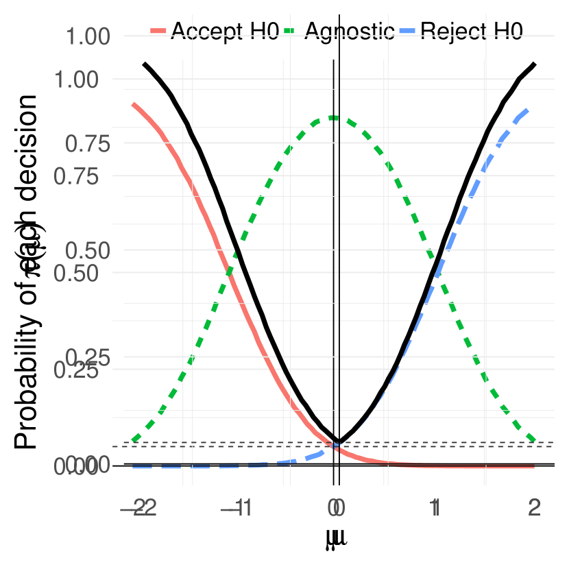
Example 2.10 (Agnostic z-test).

Let $X_{1},\ldots,X_{n}$ be an i.i.d. sample with $X_{i}\sim N(\mu,\sigma^{2})$, where $\mu\in{\mathbb{R}}:=\Theta$ and $\sigma^{2}$ is known. Let $H_{0}=\{\mu\in\Theta:\mu\leq\mu_{0}\}$ and $T=\bar{X}$ be the sample mean. Note that the conditions in Assumption 2.7 are satisfied. Furthermore, if $\alpha+\beta\leq 1$, then by taking $c_{0}=\mu_{0}-\sigma n^{-0.5}\Phi^{-1}(1-\beta)$ and $c_{1}=\mu_{0}-\sigma n^{-0.5}\Phi^{-1}(\alpha)$, one obtains that $c_{0}\leq c_{1}$, $\sup_{\theta\in H_{0}}{\mathbb{P}}_{\theta}(T>c_{1})=\alpha$ and $\sup_{\theta\in H_{1}}{\mathbb{P}}_{\theta}(T\leq c_{0})=\beta$. Therefore, it follows from Theorem 2.9 that $\phi_{T,c_{0},c_{1}}$ is an UMP $(\alpha,\beta)$-level agnostic test.

Figure 1 illustrates the probability of each decision of this test as well as its power function when $\sigma=1$, $n=10$ and $\alpha=\beta=0.05$.

Figure 1: Probability of each decision for the UMP $(0.05,0.05)$-level agnostic test for $H_{0}:\mu\leq 0$ (left) and power function for this test (right). The gray dashed horizontal line shows the values $\alpha=\beta=0.05$.

2.2 Unbiased uniformly most powerful

Besides the case studied in Assumption 2.7, there often do not exist UMP tests. For example, they might not exist when the model has nuisance parameters. This often occurs because it is possible for a test to sacrifice power in a region of $\Theta$ in order to obtain a high power in another region. However, such sacrifices might yield undesirable tests. These tests are characterized in the following passage.

An example of an undesirable test is a test that uses no data. For example, if $\alpha+\beta\leq 1$ and $U\sim\text{Uniform}(0,1)$, then $\phi^{U}:=\phi_{U,\beta,1-\alpha}$ is a test that uses no data and that attains level $(\alpha,\beta)$. Furthermore, for every $\theta_{0}\in H_{0}$, $\pi_{\phi^{U}}(\theta_{0})=\beta_{\phi^{U}}$ and also for every $\theta_{1}\in H_{1}$, $\pi_{\phi^{U}}(\theta_{1})=\alpha_{\phi^{U}}$. A generalization of this idea is to consider that a desirable test, $\phi$, should dominate trivial tests of the same level, that is, for every $\theta_{0}\in H_{0}$, $\pi_{\phi}(\theta_{0})\geq\beta_{\phi}$ and for every $\theta_{1}\in H_{1}$, $\pi_{\phi}(\theta_{1})\geq\alpha_{\phi}$. Such tests are usually called unbiased.

Definition 2.11.

An agnostic test, $\phi$, is unbiased if

$$\begin{cases}\inf_{\theta_{0}\in H_{0}}{\mathbb{P}}_{\theta_{0}}(\phi=0)=\pi_{\phi}(\theta_{0})&\geq\sup_{\theta_{1}\in H_{1}}{\mathbb{P}}_{\theta_{1}}(\phi=0)=\beta_{\phi}\\ \inf_{\theta_{1}\in H_{1}}{\mathbb{P}}_{\theta_{1}}(\phi=1)=\pi_{\phi}(\theta_{1})&\geq\sup_{\theta_{0}\in H_{0}}{\mathbb{P}}_{\theta_{1}}(\phi=0)=\alpha_{\phi}\end{cases}$$

Note that, if $\phi$ is unbiased, then $\alpha_{\phi}+\beta_{\phi}\leq 1$.

Once only unbiased tests are considered, it is often possible to find an uniformly most powerful test. In the following, Assumptions 2.14 and 2.16 present general conditions under which there exist tests that are uniformly most powerful among the unbiased tests. These conditions are the same as the ones that are typically used in the standard frequentist framework [11][p.151].

Definition 2.12.

An $(\alpha,\beta)$-level test is said to be uniformly most powerful among unbiased tests (UMPU) if, for every unbiased $(\alpha,\beta)$-size test, $\phi$, $\phi^{*}\succeq\phi$.

Notation 2.13

Let $\theta\in{\mathbb{R}}^{n}$. The $i$-th element of $\theta$ is denoted by $\theta(i)$. This notation is useful because $\theta_{i}$ is used to denote an element of $H_{i}$ and not the $i$-th element of $\theta$.

Assumption 2.14

1. For every $\theta\in\Theta$, ${\mathbb{P}}_{\theta}$ is absolutely continuous with respect to the Lebesgue measure, $\lambda$, and $f_{\theta}(x):=\frac{d{\mathbb{P}}_{\theta}}{d\lambda}(x)>0$.

2. $\theta\in{\mathbb{R}}^{n}=\Theta$ and $f_{\theta}(x)$ is in the exponential family, that is, there exists $h:{\mathbb{R}}\rightarrow{\mathbb{R}}^{n}$ such that $f_{\theta}(x)=b(x)\exp\left(\theta\cdot h(x)-a(\theta)\right)$.

3. Let $T=(h_{2}(X),\ldots,h_{n}(X))$. There exists $V(h(X))$ such that $V$ is increasing in $h_{1}(X)$ and $T$ and $V$ are independent when $\theta(1)={\theta^{*}}$.

Theorem 2.15.

Let $H_{0}=\{\theta\in\Theta:\theta(1)\leq{\theta^{*}}\}$, $\bar{\theta}\in\Theta$ be such that $\bar{\theta}(1)={\theta^{*}}$, $\alpha+\beta\leq 1$, and $c_{0},c_{1}\in{\mathbb{R}}$ be such that ${\mathbb{P}}_{\bar{\theta}}(V\leq c_{0})=\beta$ and ${\mathbb{P}}_{\bar{\theta}}(V>c_{1})=\alpha$. Under Assumption 2.14, $\phi_{V,c_{0},c_{1}}$ is an UMPU $(\alpha,\beta)$-level test.

Theorem 2.15 uses Assumption 2.14 in order to derive UMPU unilateral tests. Under the stronger conditions in Assumption 2.16 it is also possible to derive UMPU bilateral tests, as presented in theorem 2.18.

Assumption 2.16

Besides the conditions in Assumption 2.14, also include that

$$V(h_{1}(x),T)=a(T)h_{1}(x)+b(t).$$

Definition 2.17.

Let $c_{0,l},c_{1,l},c_{0,r},c_{1,r}\in{\mathbb{R}}$ be such that $c_{1,l}\leq c_{0,l}\leq c_{0,r}\leq c_{1,r}$.

$$\phi_{V,{\mathbf{c}}} =\begin{cases}1&\text{, if }V<c_{1,l}\text{ or }V>c_{1,r}\\ 0&\text{, if }c_{0,l}\leq V\leq c_{0,r}\\ \frac{1}{2}&\text{, otherwise.}\end{cases}$$

Theorem 2.18.

Let $H_{0}=\{\theta\in\Theta:\theta(1)={\theta^{*}}\}$, $\bar{\theta}\in\Theta$ be such that $\bar{\theta}(1)={\theta^{*}}$, $\alpha+\beta\leq 1$, and for each $\gamma\in(0,1)$, let $c_{\gamma,l}$ and $c_{\gamma,r}$ be such that

$$1-{\mathbb{P}}_{\bar{\theta}}(c_{\gamma,l}\leq V\leq c_{\gamma,r}) =\gamma$$

$${\mathbb{E}}_{\bar{\theta}}[V(1-{\mathbb{I}}(c_{\gamma,l}\leq V\leq c_{\gamma,r}))] =\gamma{\mathbb{E}}_{\bar{\theta}}[V]$$

Let ${\mathbf{c}}=(c_{1-\beta,l},c_{\alpha,l},c_{\alpha,r},c_{1-\beta,r})$. Under Assumption 2.16 $\phi_{V,{\mathbf{c}}}$ is an UMPU $(\alpha,\beta)$-level test.

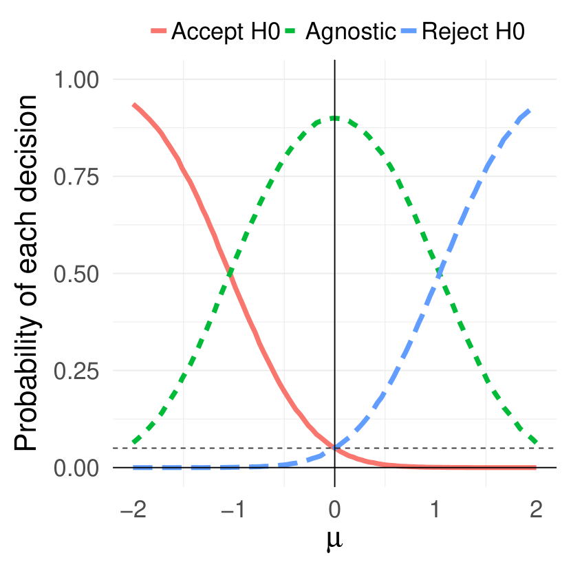
Example 2.19 (Agnostic t-test).

Let $X_{1},\ldots,X_{n}$ be an i.i.d. sample with $X_{i}\sim N(\mu,\sigma^{2})$, where $\theta=(\mu,\sigma^{2})$ and $\Theta={\rm I\!R}\times{\rm I\!R^{+}}$. Let $H_{0}^{\leq}=\{(\mu,\sigma^{2})\in\Theta:\mu\leq\mu_{0}\}$ and also $H_{0}^{=}=\{(\mu,\sigma^{2})\in\Theta:\mu=\mu_{0}\}$. Let $V=\frac{\sqrt{n}(\bar{X}-\mu_{0})}{\sqrt{(n-1)^{-1}\sum_{i=1}^{n}{(X_{i}-\mu_{0})^{2}}}}$. It follows from Lehmann and Romano [11][p.153] that $V$ satisfies the conditions in Assumptions 2.14 and 2.16 for testing $H_{0}^{\leq}$ and $H_{0}^{=}$. Therefore, if $\alpha+\beta\leq 1$, then it follows from Theorems 2.15 and 2.18 that $\phi_{V,c_{0},c_{1}}$ and $\phi_{V,{\mathbf{c}}}$ are the UMPU tests for $H_{0}^{\leq}$ and $H_{0}^{=}$. Moreover, by defining $T(X)=\frac{\sqrt{n}(\bar{X}-\mu_{0})}{\sqrt{(n-1)^{-1}\sum_{i=1}^{n}{(X_{i}-\bar{X})^{2}}}}$, it follows from Lehmann and Romano [11][p.155] that $\phi_{V,c_{0},c_{1}}$ and $\phi_{V,{\mathbf{c}}}$ are such that

$$\phi_{V,c_{0},c_{1}}(x) =\begin{cases}0&T(x)\leq t_{n-1}(\beta)\\ 1&T(x)>t_{n-1}(1-\alpha)\\ \frac{1}{2}&\text{, otherwise.}\end{cases} \phi_{V,{\mathbf{c}}}(x) =\begin{cases}0&\text{, if }|T(x)|\leq t_{n-1}(0.5(1+\beta))\\ 1&\text{, if }|T(x)|>t_{n-1}(1-0.5\alpha)\\ \frac{1}{2}&\text{, otherwise.}\end{cases}$$

where $t_{n-1}(p)$ is the $p$-quantile of a Student’s t-distribution with $n-1$ degrees of freedom. Figure 2 illustrates the probability of each decision for $\phi_{V,c_{0},c_{1}}$ and $\phi_{V,{\mathbf{c}}}$ when $\mu_{0}=0$, $\sigma^{2}=1$, $n=10$ and $\alpha=\beta=0.05$. The power of both tests at $\mu_{0}=0$ is $\beta$. Indeed, it follows from Assumption 2.14 that the power of a $(\alpha,\beta)$-size test at the border points of $H_{0}$ cannot be higher than $\min(\alpha,\beta)$.

Figure 2: Probability of each decision for $\phi_{V,c_{0},c_{1}}$ (left) and $\phi_{V,{\mathbf{c}}}$ (right) when $\mu_{0}=0$, $\sigma^{2}=1$, $n=10$ and $\alpha=\beta=0.05$.

Example 2.20 (Agnostic linear regression).

Consider a linear regression setting, that is, ${\mathbf{Y}}={\mathbb{X}}{\bm{\beta}}+{\bm{\epsilon}}$, where $d<n$, ${\bm{\epsilon}}\sim N(\textbf{0},\sigma^{2}\mathbb{I}_{d})$, ${\mathbb{X}}$ is a $n\times d$ design matrix of rank d and ${\bm{\beta}}$ is the $d\times 1$ vector with coefficients. For a fixed $k\in{\mathbb{R}}^{d}$ and $c\in{\mathbb{R}}$, let $H_{0}^{\leq}:k\cdot{\bm{\beta}}\leq c$ and $H_{0}^{=}:k\cdot{\bm{\beta}}=c$. Let $\alpha+\beta\leq 1$. By taking $\hat{{\bm{\beta}}}=({\mathbb{X}}^{t}{\mathbb{X}})^{-1}{\mathbb{X}}^{t}Y$, the least squares estimator for ${\bm{\beta}}$, it follows from Shao [19][p.416] that $V=\frac{k^{t}\hat{\beta}-c}{\sqrt{k^{t}({\mathbb{X}}^{t}{\mathbb{X}})^{-1}k}\|Y\|^{2}_{2}(n-d)^{-1}}$ satisfies the conditions in Assumptions 2.14 and 2.16. Therefore, the UMPU tests, $\phi_{V,c_{0},c_{1}}$ and $\phi_{V,{\mathbf{c}}}$, are such that

$$\phi_{V,c_{0},c_{1}}(x) =\begin{cases}0&V(x)\leq t_{n-d}(\beta)\\ 1&V(x)>t_{n-d}(1-\alpha)\\ \frac{1}{2}&\text{, otherwise.}\end{cases} \phi_{V,{\mathbf{c}}}({\mathbf{x}}) =\begin{cases}0&\text{, if }|V(x)|\leq t_{n-d}(0.5(1+\beta))\\ 1&\text{, if }|V(x)|>t_{n-d}(1-0.5\alpha)\\ \frac{1}{2}&\text{, otherwise.}\end{cases}$$

where $t_{n-d}(q)$ denotes the $q$ quantile of Student’s t-distribution with $n-d$ degrees of freedom.

3 General agnostic tests of a given level

Oftentimes, an UMPU agnostic test does not exist or is difficult to derive. In such a situation, one might be willing to use an $(\alpha,\beta)$-level test that is not uniformly most powerful. A wide class of such tests can be obtained through the p-value of standard hypothesis tests. The definition of p-value is revisited below.

Definition 3.1.

A nested family of standard tests for $H_{0}$, $\Phi$, is such that

1. For every $\phi\in\Phi$, $\phi$ is a standard test.

2. The function $g:\Phi\rightarrow[0,1]$, $g(\phi)=\alpha_{\phi}$ is bijective.

3. If $\phi_{1},\phi_{2}\in\Phi$ and $\alpha_{\phi_{1}}\leq\alpha_{\phi_{2}}$, then $\{x\in\mathcal{X}:\phi_{1}(x)=1\}\subset\{x\in\mathcal{X}:\phi_{2}(x)=1\}$.

Example 3.2.

Let $\lambda(x)=-\log\left(\frac{\sup_{{\theta_{0}}\in H_{0}}f_{{\theta_{0}}}(x)}{\sup_{\theta\in\Theta}f_{\theta}(x)}\right)$. The collection of generalized likelihood ratio tests, $\Phi=\{\phi_{\lambda,k,k}:k\geq 0\}$, is a nested family of standard tests for $H_{0}$.

Definition 3.3.

Let $\Phi$ denote a nested family of standard tests for $H_{0}$. The p-value of $\Phi$ against $H_{0}$, $p_{H_{0},\Phi}:\mathcal{X}\rightarrow[0,1]$ is such that $p_{H_{0},\Phi}(x)=\inf\{\alpha_{\phi}:\phi\in\Phi\wedge\phi(x)=1\}$.

Intuitively, if $H_{0}$ is rejected whenever the p-value is smaller than $\alpha$, then the type I error is controlled by $\alpha$. Similarly, one might expect that if $H_{0}$ is accepted whenever the p-value is larger than $1-\beta$, then the type II error is controlled by $\beta$. theorem 3.4 provides conditions under which this reasoning is valid.

Theorem 3.4.

Let $\Phi$ be a nested family of standard tests for $H_{0}$ such that, for every $\phi\in\Phi$, $\phi$ is an unbiased test. Assume that $\Theta$ is a connected space and that, for every $x\in\mathcal{X}$, ${\mathbb{P}}_{\theta}(p_{H_{0},\Phi}(x)\leq t)$ is a continuous function over $\theta$. Let $p=p_{H_{0},\Phi}$. Then, the test $\phi_{1-p,\beta,1-\alpha}$, i.e.,

$$\phi_{1-p,\beta,1-\alpha}(x) =\begin{cases}0&\text{, if $p(x)\geq 1-\beta$}\\ 1&\text{, if $p(x)<\alpha$}\\ \frac{1}{2}&\text{, otherwise.}\end{cases}$$

is a $(\alpha,\beta)$-level test for $H_{0}$.

Example 3.5 (General Linear Hypothesis in Regression Analysis).

Consider the linear regression setting (example 2.20) and the general linear hypothesis

$$H_{0}:\mathbb{K}{\bm{\beta}}={\bm{\gamma}}_{0}$$

where $\mathbb{K}$ is a $q\times d$ matrix and ${\bm{\gamma}}_{0}\in\mathbb{R}^{q}$. A particular case of this problem is the ANOVA test [16]. There exists no UMPU test for $H_{0}$ [7]. However, the F-statistic

$$F =\frac{(\mathbb{K}\widehat{{\bm{\beta}}}-{\bm{\gamma}}_{0})^{t}(\mathbb{K}(\mathbb{X}^{t}\mathbb{X})^{-1}\mathbb{K}^{t})^{-1}(\mathbb{K}\widehat{{\bm{\beta}}}-{\bm{\gamma}}_{0})q^{-1}}{({\mathbf{y}}-\mathbb{X}{\bm{\beta}})^{t}({\mathbf{y}}-\mathbb{X}{\bm{\beta}})(n-p)^{-1}}$$

is such that, for every $k\geq 0$, $\phi_{F,k,k}$ is unbiased for $H_{0}$ [14]. Furthermore, it can be shown that $p_{H_{0},\Phi}=F_{q,n-1}(F)$, where $F_{q,n-1}(\cdot)$ denotes the cumulative distribution function of a Snedecor’s F-distribution random variable with $(q,n-1)$ degrees of freedom. Since all conditions in theorem 3.4 are satisfied, $\phi_{1-F_{q,n-1}(F),\beta,1-\alpha}$ is a $(\alpha,\beta)$-level test.

Example 3.6 (Permutation Test).

Let ${\mathbf{X}}=(X_{1},\ldots,X_{m})$ and ${\mathbf{Y}}=(Y_{1},\ldots,Y_{n})$ be i.i.d. samples from continuous distributions, $F_{X}$ and $F_{Y}$. Also, consider that $H_{0}:F_{X}=F_{Y}$ and $\Theta=\{(F_{X},F_{Y}):F_{X}\mbox{ is stocastically larger than }F_{Y}\}$. Let $p_{H_{0}}({\mathbf{X}},{\mathbf{Y}})$ be a p-value based on a permutation test such that, if ${\mathbf{Y}}^{\prime}=(Y^{\prime}_{1},\ldots,Y^{\prime}_{n})$ is such that, for every $i=1,\ldots,n$, $y^{\prime}_{i}\geq y_{i}$, then $p_{H_{0}}({\mathbf{X}},{\mathbf{Y}}^{\prime})\geq p_{H_{0}}({\mathbf{X}},{\mathbf{Y}})$. It follows from Lehmann and Romano [11, Lemma 5.9.1] that $p_{H_{0}}$ is unbiased for $H_{0}$. Also, under the topology induced by the total variation metric, $\Theta$ is connected and ${\mathbb{P}}_{\theta}(p_{H_{0}}\leq t)$ is continuous over $\theta$. Conclude from theorem 3.4 that $\phi_{1-p_{H_{0}},\beta,1-\alpha}$ is a $(\alpha,\beta)$-level agnostic test.

4 Connections to region estimation

There exist several known equivalences between standard tests and region estimators [2, p.241]. For example, every region estimator is equivalent to a collection of bilateral standard tests. Also, standard tests for more general hypothesis can be obtained as the indicator that the hypothesis intercepts a region estimator. These connections are useful for providing a method of obtaining and interpreting standard hypothesis tests.

The following subsections show that similar results hold for the agnostic tests that were obtained previously. Section 4.1 presents a general method for obtaining agnostic tests from confidence regions. Furthermore, it shows how this method relates to logical coherence and to the unilateral tests in section 2. Section 4.2 presents an equivalence equivalence between nested region estimators and collections of bilateral agnostic tests.

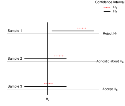
4.1 Agnostic tests based on a region estimator

An agnostic test can have other desirable properties besides controlling both the type I and type II errors. For instance, Esteves et al. [6], Stern et al. [22] show that agnostic tests can be made logically consistent. That is, it is possible to test several hypothesis using agnostic hypothesis tests in such a way that it is impossible to obtain logical contradictions between their conclusions. This property generally cannot be obtained using standard tests [8]. Logically consistent agnostic tests are connected to region estimators, as summarized below.

Definition 4.1.

A region estimator is a function $R:\mathcal{X}\rightarrow\mathcal{P}(\Theta)$.

Definition 4.2 (Agnostic test based on a region estimator).

Let $R(x)$ be a region estimator and $H_{0}\subseteq\Theta$. The agnostic test based on $R$ for testing $H_{0}$, $\phi_{H_{0},R}$ is such that

$$\phi_{H_{0},R}(x) =\begin{cases}0&\text{, if }R(x)\subseteq H_{0}\\ 1&\text{, if }R(x)\subseteq H_{0}^{c}\\ \frac{1}{2}&\text{, otherwise.}\\ \end{cases}$$

Figure 3 illustrates this procedure.

Figure 3: $\phi(x)$ is an agnostic test based on the region estimator, $R(x)$, for testing $H_{0}$.

Definition 4.3.

A collection of tests, $(\phi_{H_{0}})_{H_{0}\in\mathcal{H}}$ is based on a region estimator if there exists a region estimator, $R(x)$, such that, for every $H_{0}\in\mathcal{H}$, $\phi_{H_{0}}$ is based on $R$.

Theorem 4.4 (Esteves et al. [6]).

Let $(\phi_{H_{0}})_{H_{0}\in\sigma(\Theta)}$ be a collection of agnostic tests such that $\sigma(\Theta)$ is a $\sigma$-field over $\Theta$ and, for every $\theta\in\Theta$, $\{\theta\}\in\sigma(\Theta)$. $(\phi_{H_{0}})_{H_{0}\in\sigma(\Theta)}$ is logically consistent if and only if it is based on a region estimator.

It follows from theorem 4.4 that the collection of tests based on a region estimator is logically consistent. theorem 4.5 shows that, if this region estimator has confidence $1-\alpha$, then the tests based on it also control both the type I and II errors by $\alpha$.

Theorem 4.5.

If $R(x)$ is a region estimator for $\theta$ with confidence $1-\alpha$ and $\phi_{H_{0},R}$ is an agnostic test for $H_{0}$ based on $R$, then $\phi_{H_{0},R}$ is a $(\alpha,\alpha)$-size test.

Furthermore, the unilateral tests that were developed in Sections 2 and 3 are based on confidence regions. In order to present such regions, theorem 4.8 uses Assumptions 4.6 and 4.7.

Assumption 4.6

Let $H_{0,\theta^{*}}:\theta(1)\leq\theta^{*}$. $\left(\phi_{H_{0,\theta^{*}}}\right)_{\theta^{*}\in{\mathbb{R}}}$ is a collection of agnostic tests such that

1. If ${\theta_{1}}\leq\theta_{2}$ and $\phi_{H_{0,{\theta_{1}}}}(x)=0$, then $\phi_{H_{0,\theta_{2}}}(x)=0$

2. If ${\theta_{1}}\leq\theta_{2}$ and $\phi_{H_{0,\theta_{2}}}(x)=1$, then $\phi_{H_{0,{\theta_{1}}}}(x)=1$.

Assumption 4.7

Let $H_{0,\theta^{*}}:\theta(1)\leq\theta^{*}$. $\left(\phi_{H_{0,\theta^{*}}}\right)_{\theta^{*}\in{\mathbb{R}}}$ is a collection of agnostic tests such that for every $\theta\in\Theta$ such that $\theta(1)=\theta^{*}$, ${\mathbb{P}}_{\theta}\left(\phi_{H_{0,\theta^{*}}}=\frac{1}{2}\right)\geq 1-2\alpha$

Assumption 4.6 requires that a collection of unilateral tests satisfy a weak form of logical coherence. That is, if ${\theta_{1}}\leq\theta_{2}$ and the collection of tests accepts that $\theta\leq{\theta_{1}}$, then it accepts that $\theta\leq\theta_{2}$. Similarly, if ${\theta_{1}}\leq\theta_{2}$ and the collection of tests rejects that $\theta\leq\theta_{2}$, then it also rejects that $\theta\leq{\theta_{1}}$. Assumption 4.7 requires that, for every test in the collection, the probability of the no-decision alternative in the border point of $H_{0}$ is at least $1-2\alpha$. Theorem 4.8 shows that a collection of unilateral tests that satisfy Assumptions 4.6 and 4.7 is based on a confidence region of confidence $1-2\alpha$.

Theorem 4.8.

For each, $\theta^{*}$, let $H_{0,\theta^{*}}:\theta(1)\leq\theta^{*}$. If $\left(\phi_{H_{0,\theta^{*}}}\right)_{\theta^{*}\in{\mathbb{R}}}$ satisfies Assumption 4.6, then there exists a region estimator, $R(x)$, such that, for every $\theta^{*}$, $\phi_{H_{0,\theta^{*}}}$ is based on $R(x)$. Furthermore, if Assumption 4.7 holds, then $R(x)$ is a confidence region for $\theta$ with confidence $1-2\alpha$.

It is possible to use theorems 4.5 and 4.8 in order to extend a collection of unilateral tests to a larger collection of tests. If the collection of unilateral tests satisfies Assumptions 4.6 and 4.7, then it follows from theorem 4.8 that these tests are based on a region estimator, $R(X)$, with confidence $1-2\alpha$. Therefore, it follows from theorem 4.5 that, for every $H_{0}$ of the type $\theta(1)\in\Theta_{0}\subseteq{\mathbb{R}}$, the test for $H_{0}$ based on $R(X)$ has size $(2\alpha,2\alpha)$. Furthermore, it follows from theorem 4.4 that the collection of these tests is logically coherent. corollary 4.9 summarizes these conclusions.

Corollary 4.9.

For each, $\theta^{*}$, let $H_{0}:\theta(1)\leq\theta^{*}$. Also, assume that $\left(\phi_{H_{0,\theta^{*}}}\right)_{\theta^{*}\in{\mathbb{R}}}$ satisfies Assumptions 4.6 and 4.7. Let $R(X)$ be such as in theorem 4.8. Consider the collection of agnostic tests $(\phi_{H_{0,{\Theta_{0}}},R})_{{\Theta_{0}}\subset{\mathbb{R}}}$, where $H_{0,{\Theta_{0}}}:\theta(1)\in{\Theta_{0}}$ (recall Definition 4.2). Then

1. this collection is logically coherent,

2. each test is this collection has size $(2\alpha,2\alpha)$, and

3. this collection is an extension of the collection $\left(\phi_{H_{0,\theta^{*}}}\right)_{\theta^{*}\in{\mathbb{R}}}$

Under weak conditions, the tests that were developed in theorems 2.9 and 2.15 satisfy Assumptions 4.6 and 4.7. As a result, they can be used in theorems 4.8 and 4.9. These results are presented in corollaries 4.10 and 4.13 and illustrated in examples 4.11 and 4.14.

Corollary 4.10.

Consider the setting of theorem 2.9, and let $H_{0,\theta^{*}}:\theta\leq\theta^{*}$. The collection $\phi_{H_{0,\theta^{*}}}$ of UMP $(\alpha,\alpha)$-level test presented in theorem 2.9 is based on a region estimator, $R(X)$. Furthermore, if $T$ is such that ${\mathbb{P}}_{\theta}(T\leq t)$ is continuous over $\theta$, then $R(X)$ has confidence $1-2\alpha$ for $\theta$.

Example 4.11 (Agnostic z-test).

Consider again example 2.10. For each $\mu^{*}\in{\mathbb{R}}$, let $H_{0,\mu^{*}}:\mu\leq\mu^{*}$. Let $\alpha\leq 0.5$ and $\left(\phi_{H_{0,\mu^{*}}}\right)_{\mu^{*}\in{\mathbb{R}}}$ be the collection of UMP $(\alpha,\alpha)$-level tests in example 2.10. By defining the constants $a_{1}=\sigma n^{-0.5}\Phi^{-1}(1-\alpha)$ and $a_{2}=\sigma n^{-0.5}\Phi^{-1}(\alpha)$, note that $\phi_{H_{0,\mu^{*}}}=\phi_{\bar{X},\mu^{*}-a_{1},\mu^{*}-a_{2}}$. It follows that $\left(\phi_{H_{0,\mu^{*}}}\right)_{\mu^{*}\in{\mathbb{R}}}$ is based on the region estimator $R(X)=[\bar{X}-a_{1},\bar{X}-a_{2}]$, which is a $1-2\alpha$ confidence interval for $\mu$.

Assumption 4.12

For each $\theta^{*}\in{\mathbb{R}}$, let $V_{\theta^{*}}$ be such as in Assumption 2.14 when $\theta(1)=\theta^{*}$. There exists a function, $g(v,\theta)$, which is decreasing over $\theta$ and such that $g(V_{\theta},\theta)$ is ancillary.

Corollary 4.13.

For each $\theta^{*}\in\mathbb{R}$, let $H_{0,\theta^{*}}:\theta(1)\leq\theta^{*}$. Under Assumption 2.14 and $\alpha\leq 0.5$, let $\phi_{H_{0,\theta^{*}}}$ be the UMPU $(\alpha,\alpha)$-level test presented in theorem 2.15. Under Assumption 4.12, the collection $\left(\phi_{H_{0,\theta^{*}}}\right)_{\theta^{*}\in\Theta}$ is based on a region estimator, $R(X)$, which has confidence $1-2\alpha$ for $\theta$.

Example 4.14 (Agnostic t-test).

Consider again example 2.19. For each $\mu^{*}\in{\mathbb{R}}$, let $H_{0,\mu^{*}}:\mu\leq\mu^{*}$. Let $\alpha\leq 0.5$ and $\left(\phi_{H_{0,\mu^{*}}}\right)_{\mu^{*}\in{\mathbb{R}}}$ be the collection of UMP $(\alpha,\alpha)$-level tests in example 2.19. By defining $S=\sqrt{(n-1)^{-1}\sum_{i=1}^{n}{(X_{i}-\bar{X})^{2}}}$, $a_{1}=n^{-0.5}St_{n-1}^{-1}(1-\alpha)$ and $a_{2}=n^{-0.5}St_{n-1}^{-1}(\alpha)$, note that $\phi_{H_{0,\mu^{*}}}=\phi_{\bar{X},\mu^{*}-a_{1},\mu^{*}-a_{2}}$. It follows that $\left(\phi_{H_{0,\mu^{*}}}\right)_{\mu^{*}\in\Theta}$ is based on the region estimator $R(X)=[\bar{X}-a_{1},\bar{X}-a_{2}]$, which is a $1-2\alpha$ confidence interval for $\mu$.

4.2 Agnostic tests based on nested region estimators

Contrary to the unilateral tests, the bilateral tests in section 2 are not based on region estimators. Indeed, while these bilateral tests can accept a precise hypothesis, this feature cannot be obtained in tests based on region estimators. However, similarly to the case for standard tests, there exists an equivalence between collections of bilateral agnostic tests and pairs of nested region estimators. Indeed, it is possible to obtain from one another a nested pair of $1-\alpha$ and $\beta$ confidence regions and a collection of bilateral $(\alpha,\beta)$-size tests. Definition 4.15 prepares for this equivalence, which is established in theorem 4.17.

Definition 4.15 (Agnostic test based on nested region estimators).

Let $R_{1}(x)$ and $R_{2}(x)$ be region estimators such that, $R_{1}(x)\subseteq R_{2}(x)$ and $H_{0}\subseteq\Theta$. The agnostic test based on $R_{1}$ and $R_{2}$ for testing $H_{0}$, $\phi_{H_{0},R_{1},R_{2}}$, is

$$\phi_{H_{0},R_{1},R_{2}}(x) =\begin{cases}0&\text{, if }H_{0}\subseteq R_{1}\\ 1&\text{, if }R_{2}\subseteq H_{0}^{c}\\ \frac{1}{2}&\text{, otherwise.}\\ \end{cases}$$

Figure 4 illustrates $\phi_{H_{0},R_{1},R_{2}}$ when $H_{0}:\theta={\theta_{0}}$.

Figure 4: Illustration of the agnostic test based on $R_{1}$ and $R_{2}$ (definition 4.15) when $H_{0}:\theta={\theta_{0}}$.

Example 4.16 (Agnostic t-test).

Consider example 2.19. For each $\mu^{*}\in{\mathbb{R}}$, let $H_{0,\mu^{*}}:\mu=\mu^{*}$. The UMPU agnostic test is based on the region estimators

$$R_{1}(x) =\left[\bar{X}-t_{n-1}(0.5(1+\beta))\sqrt{S^{2}/n},\bar{X}+t_{n-1}(0.5(1+\beta))\sqrt{S^{2}/n}\right]\text{, and}$$

$$R_{2}(x) =\left[\bar{X}-t_{n-1}(1-0.5\alpha)\sqrt{S^{2}/n},\bar{X}+t_{n-1}(1-0.5\alpha)\sqrt{S^{2}/n}\right]$$

Theorem 4.17.

For each $\theta^{*}$, let $H_{0,\theta^{*}}:\theta(1)=\theta^{*}$.

1. If $R_{1}(x)\subseteq R_{2}(x)$ are confidence regions for $\theta$ with confidence $1-\beta$ and $\alpha$, then for every $\theta^{*}\in{\mathbb{R}}$, $\phi_{H_{0,\theta^{*}},R_{1},R_{2}}$ is a $(\alpha,\beta)$-size test.

2. Let $\left(\phi_{H_{0,\theta^{*}}}\right)_{\theta^{*}\in{\mathbb{R}}}$ be a collection of $(\alpha,\beta)$-size tests. If for every $\theta\in\Theta$ such that $\theta(1)=\theta^{*}$, ${\mathbb{P}}_{\theta}(\phi_{H_{0,\theta^{*}}}=0)=\beta$ and ${\mathbb{P}}_{\theta}(\phi_{H_{0,\theta^{*}}}=1)=\alpha$, then there exist region estimators, $R_{1}(x)$ and $R_{2}(x)$, such that $R_{1}(x)\subseteq R_{2}(x)$, $R_{1}(x)$ and $R_{2}(x)$ are confidence regions for $\theta$ with, respectively, confidence $1-\beta$ and $\alpha$ and such that $\phi_{H_{0,\theta^{*}}}$ is based on $R_{1}(x)$ and $R_{2}(x)$.

5 Consistent agnostic tests

A sequence of agnostic tests, which is indexed on the sample size, is consistent if there exists a large enough sample such that, with high probability, the test accepts $H_{0}$ under $H_{0}$ and reject $H_{1}$ under $H_{1}$. That is, a sequence of agnostic tests is consistent if the respective sequence of power functions converges to $1$ as the sample size goes to infinity. This notion is formalized in definition 5.1.

Definition 5.1.

A sequence of agnostic tests for $H_{0}$, $(\phi_{n})_{n\in\mathbb{N}}$, is consistent if, for every $\theta\in\Theta$, $\lim_{n\rightarrow\infty}\pi_{\phi_{n}}(\theta)=1$.

Under a wide variety of models, it is impossible to obtain consistent agnostic tests. A class of such models is described in Assumption 5.2.

Assumption 5.2 (Non-separability between $H_{0}$ and $H_{1}$)

1. $\Theta$ is connected.

2. $H_{0}\notin\{\emptyset,\Theta\}$.

3. $(\phi_{n})_{n\in\mathbb{N}}$ is a sequence of agnostic tests for $H_{0}$ such that, for every $n\in\mathbb{N}$ and $i\in\left\{0,\frac{1}{2},1\right\}$, ${\mathbb{P}}_{\theta}(\phi_{n}=i)$ is continuous over $\theta$.

Assumption 5.2 is met in the examples presented in sections 2 and 3. Theorem 5.3 shows that, under Assumption 5.2, it is impossible to obtain a consistent sequence of hypothesis test.

Theorem 5.3.

Under Assumption 5.2, if $(\phi_{n})_{n\in\mathbb{N}}$ is a sequence of $(\alpha,\beta)-size$ tests, where $\max(\alpha,\beta)<1$, then $(\phi_{n})_{n\in\mathbb{N}}$ is not consistent. Furthermore, under the same assumption, if $\lim_{n\rightarrow\infty}\alpha_{n}=0$, $\lim_{n\rightarrow\infty}\beta_{n}=0$ and $(\phi_{n})_{n\in\mathbb{N}}$ is a sequence of $(\alpha_{n},\beta_{n})$-size tests, then for some $\theta\in\Theta$, $\lim_{n\rightarrow\infty}{\mathbb{P}}_{\theta}\left(\phi_{n}=\frac{1}{2}\right)=1$.

Despite theorem 5.3, consistency can be obtained by relaxing the control over the test’s errors. In particular, one might drop the requirement that the type II error probability be controlled uniformly over all points in the alternative hypothesis. The remainder of this section explores alternative methods of controlling the type II error probabilities.

One alternative way to control the type II error probabilities is to require solely that $\sup_{\theta\in{H_{1}^{\prime}}}{\mathbb{P}}_{\theta}(\phi=0)\leq\beta$, where ${H_{1}^{\prime}}$ is a subset of $H_{1}$ which is relevant for the practitioner. One procedure to choose ${H_{1}^{\prime}}$ in practice is to determine a desired effect size through expert knowledge elicitation. The effect size is often easier to interpret than the value of the parameter itself. This procedure is similar to what is often done in power calculations [16].

Example 5.4.

(Agnostic linear regression) Consider the linear regression setting in example 2.20. Also, one wishes to test the hypothesis $H_{0}:\beta_{k}=0$ with the agnostic hypothesis test, $\phi_{T,c_{0},c_{1}}$ (definition 2.8), where $T=\left|\frac{\widehat{\beta}_{k}}{\sqrt{\widehat{{\mathbb{V}}}[\widehat{\beta}_{k}]}}\right|$. For every $\theta\in\Theta$, the probability that $\phi_{T,c_{0},c_{1}}$ accepts $H_{0}$ is

$${\mathbb{P}}_{\theta}\left(T\leq c_{0}\right) ={\mathbb{P}}_{\theta}\left(-c_{0}\leq\frac{\widehat{\beta}_{k}}{\sqrt{\widehat{{\mathbb{V}}}[\widehat{\beta}_{k}]}}\leq c_{0}\right)={\mathbb{P}}_{\theta}\left(-c_{0}\leq\frac{\frac{\widehat{\beta}_{k}-\beta_{k}}{\sqrt{{\mathbb{V}}[\widehat{\beta}_{k}]}}+\frac{\beta_{k}}{\sqrt{{\mathbb{V}}[\widehat{\beta}_{k}]}}}{\sqrt{\widehat{{\mathbb{V}}}[\widehat{\beta}_{k}]{{\mathbb{V}}}[\widehat{\beta}_{k}]^{-1}}}\leq c_{0}\right)$$

$$={\mathbb{P}}\left(-c_{0}\leq T_{n-d-1,\delta_{k}}\leq c_{0}\right),$$ (1)

where $T_{p,\delta}$ has a non-central $t$-distribution with $p$ degrees of freedom and non-centrality parameters $\delta$, that is, $\delta_{k}=\frac{\beta_{k}}{\sqrt{{\mathbb{V}}[\widehat{\beta}_{k}]}}=\frac{d_{k}}{\sqrt{a}_{k}}$, $a_{k}$ is the $k$-th element of the diagonal of the matrix $({\mathbb{X}}^{t}{\mathbb{X}})^{-1}$, and $d_{k}=\frac{\beta_{k}}{\sigma}$ is the Cohen’s $d$ effect size of the $k$-th variable on $Y$ [4].

A practitioner can determine a desired Cohen’s effect size value, $d_{k}^{*}$ and a $\beta\in(0,1)$, and use Equation 1 to choose $c_{0}$ such that the type II error is $\beta$ when the effect size is $d_{k}^{*}$. Since, when $\delta>\delta^{\prime}$, $T_{p,\delta}$ stochastically dominates $T_{p,\delta^{\prime}}$ this procedure guarantees that

$$\sup_{\theta\in{H_{1}^{\prime}}}{\mathbb{P}}_{\theta}(\phi=0)=\beta,$$

where ${H_{1}^{\prime}}=\{\theta\in\Theta:\delta_{k}\sqrt{a_{k}}\geq d_{k}^{*}\}$. That is, type II error probabilities are controlled by $\beta$ for every parameter value with effect size greater or equal to $d_{k}^{*}$. Note that, when $d_{k}^{*}=0$, the test which is obtained is the standard $(\alpha,\beta)$-level test for $H_{0}^{=}$ in Example 2.20 when $k=(0,\ldots,0,1,0,\ldots,0)$ and $c=0$.

The next example applies the derivation in Example 5.4 to a real dataset.

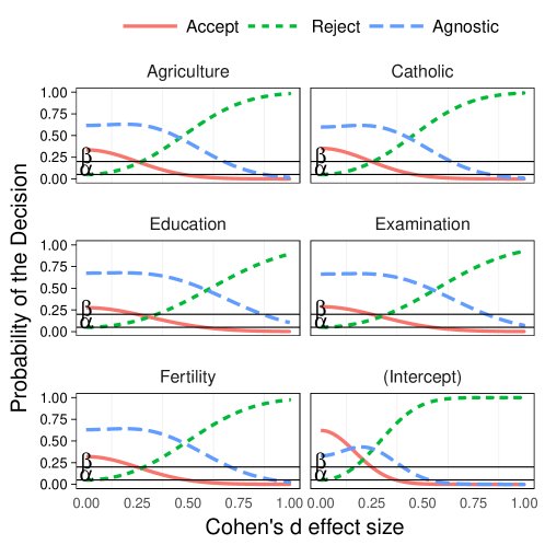
Example 5.5.

The Swiss Fertility and Socioeconomic Indicators (1888) Data [15], contains a fertility measure and socio-economic indicators for 47 French-speaking provinces of Switzerland. Table 1 presents the estimates of regressing the infant mortality rate over the other covariates using $d_{k}^{*}=0.25$, for every $k$, $\alpha=0.05$, and $\beta=0.2$. The analysis indicates that both the agriculture index of a province and the percentage of catholics on it are not associated to its infant mortality rate. On the other hand, there is an association between fertility and infant mortality rate. Finally, it is not possible to assert whether education and examination (percentage of draftees receiving highest mark on army examination) are associated to the response variable. Figure 5 shows the probability of each decision as a function of Cohen’s $d$ effect size.

	Estimate	Std. Error	t-value	p-value	Decision
(Intercept)	8.667	5.435	1.595	0.119	Accept
Fertility	0.151	0.054	2.822	0.007	Reject
Agriculture	-0.012	0.028	-0.418	0.678	Accept
Examination	0.037	0.096	0.385	0.702	Agnostic
Education	0.061	0.085	0.719	0.476	Agnostic
Catholic	0.001	0.015	0.005	0.996	Accept

Table 1: Agnostic regression analysis over the Swiss dataset (example 5.5).

Figure 5: Probability of each decision for the regression coefficients on the Swiss dataset (example 5.5).

While controlling the type II error probabilities only for a class of effect sizes, such as illustrated in examples 5.4 and 5.5, it is possible to obtain a consistent sequence of agnostic hypothesis tests. Example 5.6 illustrates this possibility in a bilateral $z$-test.

Example 5.6.

Let $X_{1},\ldots,X_{n}$ be a i.i.d. sample with $X_{i}\sim N(\mu,\sigma^{2})$, where $\mu\in{\mathbb{R}}$ and $\sigma^{2}$ is known. Let $H_{0}:\mu=0$, $\alpha_{n}=\beta_{n}=\exp(-o(n))$, $a_{n}=\frac{-\Phi^{-1}(0.5\alpha_{n})\sigma}{\sqrt{n}}$, $b_{n}$ be such that $b_{n}\leq a_{n}$ and $b_{n}^{-1}=o(\sqrt{n})$, ${\mathbf{c}}_{n}=(-a_{n},-b_{n},b_{n},a_{n})$, and $\gamma_{n}=b_{n}+\left(\frac{-2\log(\sqrt{2\pi}\beta_{n})}{n}\right)^{0.5}$. The agnostic test $\phi_{\bar{X}_{n},{\mathbf{c}}_{n}}$ controls the type I error by $\alpha_{n}$, and controls the type II error over $H_{1}^{*}:|\mu|>\gamma_{n}$ by $\beta_{n}$. Furthermore, for every $\mu\in{\mathbb{R}}$, $\lim_{n\rightarrow\infty}\pi_{\phi_{\bar{X}_{n},{\mathbf{c}}_{n}}}(\mu)=1$. That is, $\left(\phi_{\bar{X}_{n},{\mathbf{c}}_{n}}\right)_{n\in\mathbb{N}}$ is consistent.

Example 5.6 shows that, if a sequence of tests doesn’t control the type II error probabilities in a neighborhood of $H_{0}$, then it can be consistent. This occurs because, contrary to $H_{0}$ and $H_{1}$ that satisfy Assumption 5.2, $H_{0}$ and $H_{1}^{*}$ are “probabilistically separated”. Also note that, since $\lim_{n\rightarrow\infty}\gamma_{n}=0$, for every $\theta\in H_{1}$, there exists an $n^{*}$ after which the error II probability for $\theta$ is controlled by $\beta_{n}$.

6 Final remarks

Since agnostic tests control the type I and II error probabilities, their outcomes are more interpretable than the ones obtained using standard hypothesis tests. This paper provides several procedures to construct agnostic tests. In several statistical models, (unbiased) uniformly most powerful agnostic tests are obtained. When such tests are unavailable, an alternative that is based on standard p-values is presented. The paper also provides several links between region estimators and agnostic tests, which shows in particular that $(\alpha,\beta)$-level tests can be fully coherent from a logical perspective. Finally, we have shown that although one cannot obtain consistency in agnostic tests that control type I and type II error probabilities uniformly, this goal can be achieved by relaxing the control of the type II error probabilities.

An R package that implements several of the agnostic tests developed here is available at https://github.com/vcoscrato/agnostic.

7 Acknowledgments

This was partially funded by Fundação de Amparo à Pesquisa do Estado de São Paulo (2017/03363-8).

8 Demonstrations

Definition 8.1.

Let $g_{0}(x)={\mathbb{I}}(x=0)$ and $g_{1}(x)={\mathbb{I}}(x=1)$.

Lemma 8.2.

For every agnostic test, $\phi$,

1. $g_{0}(\phi)$ and $g_{1}(\phi)$ are standard tests.

2. for every $\theta\in\Theta$, ${\mathbb{P}}_{\theta}(g_{0}(\phi)=1)={\mathbb{P}}_{\theta}(\phi=0)$ and ${\mathbb{P}}_{\theta}(g_{1}(\phi)=1)={\mathbb{P}}_{\theta}(\phi=1)$.

3. If $\phi$ is unbiased, then $g_{1}(\phi)$ is unbiased for $H_{0}$ and $g_{0}(\phi)$ is unbiased for $H^{*}_{0}=H_{1}$.

Proof 8.3 (Proof of lemma 8.2).

The first two items follow directly from definition 2.2 and the definitions of $g_{0}$ and $g_{1}$. Next, if $\phi$ is unbiased, then $\alpha_{\phi}+\beta_{\phi}\leq 1$. Also,

$$\sup_{\theta_{1}\in H_{1}}{\mathbb{P}}_{\theta_{1}}(g_{0}(\phi)=1) =\sup_{\theta_{1}\in H_{1}}{\mathbb{P}}_{\theta_{1}}(\phi=0)=\beta_{\phi}$$

$${\mathbb{P}}_{\theta_{0}}(g_{0}(\phi)=1) ={\mathbb{P}}_{\theta_{0}}(\phi=0)\geq\beta_{\phi} \text{for every }\theta_{0}\in H_{0}$$

That is, $g_{0}(\phi)$ is unbiased for $H^{*}_{0}$. Similarly, $g_{1}(\phi)$ is unbiased for $H_{0}$.

Lemma 8.4.

Let $c,c_{0},c_{1}\in{\mathbb{R}}$, $c_{0}\leq c_{1}$ and $\phi$ be an agnostic test. Also, define $H_{0}:\theta_{0}\leq\theta^{*}$ and $H_{1}:\theta>\theta^{*}$, and let $\theta_{0}\in H_{0}$ and $\theta_{1}\in H_{1}$. Under Assumption 2.7,

1. If ${\mathbb{P}}_{\theta^{*}}(\phi_{T,c_{0},c_{1}}=1)\geq{\mathbb{P}}_{\theta^{*}}(\phi=1)$, then ${\mathbb{P}}_{\theta_{1}}(\phi_{T,c_{0},c_{1}}=1)\geq{\mathbb{P}}_{\theta_{1}}(\phi=1).$

2. If $\beta_{\phi_{T,c_{0},c_{1}}}\geq\beta_{\phi}$, then ${\mathbb{P}}_{\theta_{0}}(\phi_{T,c_{0},c_{1}}=0)\geq{\mathbb{P}}_{\theta_{0}}(\phi=0).$

3. If ${\mathbb{P}}_{\theta^{*}}(\phi_{T,c,c}=1)={\mathbb{P}}_{\theta^{*}}(\phi=1)$, then $\phi_{T,c,c}\succeq\phi$.

Proof 8.5.

1. Let $\theta_{1}\in H_{1}$. Note that $g_{1}(\phi_{T,c_{0},c_{1}})=\phi_{T,c_{1},c_{1}}$. Furthermore, it follows from Lemma 8.2 that ${\mathbb{P}}_{\theta^{*}}(g_{1}(\phi_{T,c_{0},c_{1}})=1)\geq{\mathbb{P}}_{\theta^{*}}(g_{1}(\phi)=1)$. Therefore, by defining $H_{0}^{*}:\theta=\theta^{*}$ and $H_{1}^{*}:\theta=\theta_{1}$, it follows from Assumption 2.7.2 and the Neyman-Pearson lemma that ${\mathbb{P}}_{\theta_{1}}(g_{1}(\phi_{T,c_{0},c_{1}})=1)\geq{\mathbb{P}}_{\theta_{1}}(g_{1}(\phi)=1)$. The inequality ${\mathbb{P}}_{\theta_{1}}(\phi_{T,c_{0},c_{1}}=1)\geq{\mathbb{P}}_{\theta_{1}}(\phi=1)$ follows from Lemma 8.2.

2. Let $\theta_{0}\in H_{0}$. Note that $g_{0}(\phi_{T,c_{0},c_{1}})=1-\phi_{T,c_{0},c_{0}}$. Furthermore, it follows from Lemma 8.2 that $\sup_{\theta_{1}\in H_{1}}{\mathbb{P}}_{\theta_{1}}(g_{0}(\phi_{T,c_{0},c_{1}})=1)\geq\sup_{\theta_{1}\in H_{1}}{\mathbb{P}}_{\theta_{1}}(g_{0}(\phi)=1)$ Therefore, by taking $H_{0}^{*}=H_{1}$ and $H_{1}^{*}=H_{0}$, it follows from Assumption 2.7.2 and the Karlin-Rubin theorem that ${\mathbb{P}}_{\theta_{0}}(g_{1}(\phi_{T,c_{0},c_{1}})=1)\geq{\mathbb{P}}_{\theta_{0}}(g_{1}(\phi)=1)$. It follows from Lemma 8.2 that ${\mathbb{P}}_{\theta_{0}}(\phi_{T,c_{0},c_{1}}=0)\geq{\mathbb{P}}_{\theta_{0}}(\phi=0)$.

3. It follows from Lemma 8.4.1 that, for every $\theta_{1}\in H_{1}$, ${\mathbb{P}}_{\theta_{1}}(\phi_{T,c,c}=1)\geq{\mathbb{P}}_{\theta_{1}}(\phi=1)$. Next, obtain from ${\mathbb{P}}_{\theta^{*}}(\phi_{T,c,c}=1)={\mathbb{P}}_{\theta^{*}}(\phi=1)$ and $\phi_{T,c,c}$ being a standard test, that ${\mathbb{P}}_{\theta^{*}}(\phi_{T,c,c}=0)\geq{\mathbb{P}}_{\theta^{*}}(\phi=0)$. It follows from Lemma 8.2 that ${\mathbb{P}}_{\theta^{*}}(g_{0}(\phi_{T,c,c})=1)\geq{\mathbb{P}}_{\theta^{*}}(g_{0}(\phi)=1)$. By taking $H_{0}:\theta=\theta^{*}$ and $H_{1}:\theta=\theta_{0}$, it follows from Assumption 2.7.2 and the Neyman-Pearson lemma that ${\mathbb{P}}_{\theta_{0}}(g_{1}(\phi_{T,c,c})=1)\geq{\mathbb{P}}_{\theta_{0}}(g_{1}(\phi)=1)$. Obtain from Lemma 8.2 that ${\mathbb{P}}_{\theta_{0}}(\phi_{T,c,c}=0)\geq{\mathbb{P}}_{\theta_{1}}(\phi=0)$. Conclude that $\phi_{T,c,c}\succeq\phi$.

Proof 8.6 (Proof of Theorem 2.9).

Let $\phi$ be an arbitrary $(\alpha,\beta)$-size agnostic test.

1. Conclude from Assumption 2.7 that

   $$P_{\theta^{*}}(\phi_{T,c_{0},c_{1}}=1) =\alpha\geq\alpha_{\phi}\geq{\mathbb{P}}_{\theta^{*}}(\phi=1)$$

   $$\beta_{\phi_{T,c_{0},c_{1}}} =\beta\geq\beta_{\phi}$$ (2)

   It follows from item 1 and Lemma 8.4 that $\phi_{T,c_{0},c_{1}}\succeq\phi$. Since $\phi$ was arbitrary, conclude that $\phi_{T,c_{0},c_{1}}$ is an UMP $(\alpha,\beta)$-level agnostic test.

2. Either there exists $c\in[c_{1},c_{0}]$ such that ${\mathbb{P}}_{\theta^{*}}(\phi_{T,c,c}=1)={\mathbb{P}}_{\theta^{*}}(\phi=1)$ or there exists no such $c$. If there exists such a $c$, then it follows from Lemma 8.4 that $\phi_{T,c,c}\succeq\phi$. Next, assume there exists no such $c$. Note that $\phi$ has size $(\alpha,\beta)$ and, therefore,

   $${\mathbb{P}}_{\theta^{*}}(\phi_{T,c_{0},c_{0}}=1)=\alpha\geq{\mathbb{P}}_{\theta^{*}}(\phi=1).$$

   Since ${\mathbb{P}}_{\theta^{*}}(\phi_{T,c,c}=1)$ decreases continuously over $c$, conclude that

   $${\mathbb{P}}_{\theta^{*}}(\phi_{T,c_{1},c_{1}}=1) \geq{\mathbb{P}}_{\theta^{*}}(\phi=1)$$

   $$\beta_{\phi_{T,c_{1},c_{1}}}=\beta \geq\beta_{\phi}$$ (3)

   Conclude from item 2 and Lemma 8.4 that $\phi_{T,c_{1},c_{1}}\succeq\phi$.

Lemma 8.7.

Let $c,c_{0},c_{1}\in{\mathbb{R}}$, $c_{0}\leq c_{1}$ and $\phi$ be an unbiased test. Define $H_{0}:\theta(1)\leq\theta^{*}$ and $H_{1}:\theta(1)>\theta^{*}$ and let $\bar{\theta}\in\Theta$ be such that $\theta(1)=\theta^{*}$. Under Assumption 2.14,

1. If ${\mathbb{P}}_{\bar{\theta}}(\phi_{V,c_{0},c_{1}}=1)\geq{\mathbb{P}}_{\bar{\theta}}(\phi=1)$, then $\forall\theta_{1}\in H_{1}$, $\pi_{\phi_{V,c_{0},c_{1}}}(\theta_{1})\geq\pi_{\phi}(\theta_{1})$.

2. If ${\mathbb{P}}_{\bar{\theta}}(\phi_{V,c_{0},c_{1}}=0)\geq\beta_{\phi}$, then $\forall\theta_{0}\in H_{0}$, $\pi_{\phi_{V,c_{0},c_{1}}}(\theta_{0})\geq\pi_{\phi}(\theta_{0})$.

Proof 8.8.

1. Let $\theta_{1}\in H_{1}$. We wish to show that ${\mathbb{P}}_{\theta_{1}}(g_{1}(\phi_{V,c_{0},c_{1}})=1)\geq{\mathbb{P}}_{\theta_{1}}(g_{1}(\phi)=1)$, Since $g_{1}(\phi_{V,c_{0},c_{1}})$ and $g_{1}(\phi)$ are standard tests, our strategy is to obtain the inequality from Lehmann and Romano [11][p.151]. In order to obtain this result, Assumption 2.14 is used to show that $g_{1}(\phi_{V,c_{0},c_{1}})$ satisfies the required conditions.

   Let $\Theta^{*}=\{\theta\in\Theta:\theta(1)\geq\bar{\theta}\}$. Note that $g_{1}(\phi_{V,c_{0},c_{1}})=\phi_{V,c_{1},c_{1}}$. Also, it follows from Lemma 8.2 that $g_{1}(\phi)$ is unbiased for $H_{0}$ under $\Theta$. Since $H_{0}$ is more restrictive under $\Theta^{*}$, $g_{1}(\phi)$ is also unbiased for $H_{0}$ under $\Theta^{*}$. Moreover, it follows from Lemma 8.2 that ${\mathbb{P}}_{\bar{\theta}}(g_{1}(\phi_{V,c_{0},c_{1}})=1)\geq{\mathbb{P}}_{\bar{\theta}}(g_{1}(\phi)=1)$. It follows from Assumption 2.14 that, under $\Theta^{*}$, $\alpha_{g_{1}(\phi_{V,c_{0},c_{1}})}\geq\alpha_{g_{1}(\phi)}$. Putting all of the above conditions together, conclude that ${\mathbb{P}}_{\theta_{1}}(g_{1}(\phi_{V,c_{0},c_{1}})=1)\geq{\mathbb{P}}_{\theta_{1}}(g_{1}(\phi)=1)$ by applying Lehmann and Romano [11][p.151] in $\Theta^{*}$. It follows directly from Lemma 8.2 that ${\mathbb{P}}_{\theta_{1}}(\phi_{V,c_{0},c_{1}}=1)\geq{\mathbb{P}}_{\theta_{1}}(\phi=1)$, which is equivalent to, $\pi_{\phi_{V,c_{0},c_{1}}}(\theta_{1})\geq\pi_{\phi}(\theta_{1})$.

2. Let $\theta_{0}\in\{\theta\in\Theta:\theta(1)<\theta^{*}\}.$ Note that $g_{0}(\phi_{V_{c}0,c_{1}})=1-\phi_{V,c_{0},c_{0}}$. Also, it follows from Lemma 8.2 that $g_{0}(\phi)$ is unbiased for $H_{0}^{*}=H_{1}$. Also, obtain from Lemma 8.2 and Assumption 2.14.2 that ${\mathbb{P}}_{\bar{\theta}}(g_{0}(\phi_{V,c_{0},c_{1}})=1)\geq\sup_{\theta_{1}\in\Theta_{1}\cup\{\theta\}}{\mathbb{P}}_{\theta_{1}}(g_{0}(\phi)=1)$. Therefore, by taking $H_{0}^{*}:\theta(1)\geq\theta^{*}$, it follows from from Assumption 2.14 and Lehmann and Romano [11][p.151] that ${\mathbb{P}}_{\theta_{0}}(g_{0}(\phi_{V,c_{0},c_{1}})=1)\geq{\mathbb{P}}_{\theta_{0}}(g_{0}(\phi)=1)$. Conclude from Lemma 8.2 that ${\mathbb{P}}_{\theta_{0}}(\phi_{V,c_{0},c_{1}}=0)\geq{\mathbb{P}}_{\theta_{0}}(\phi=0)$. Since $\theta_{0}$ was arbitrary in $H_{1}^{*}$, conclude from Assumption 2.14.2 that, for every $\theta_{0}\in\overline{H_{1}^{*}}=H_{0}$, ${\mathbb{P}}_{\theta_{0}}(\phi_{V,c_{0},c_{1}}=0)\geq{\mathbb{P}}_{\theta_{0}}(\phi=0)$, that is, $\pi_{\phi_{V,c_{0},c_{1}}}(\theta_{0})\geq\pi_{\phi}(\theta_{0})$.

Proof 8.9 (Proof of Theorem 2.15).

Since $\alpha+\beta\leq 1$, obtain $c_{0}\leq c_{1}$. It follows from Assumption 2.14 that $\phi_{V,c_{0},c_{1}}$ is a $(\alpha,\beta)$-level test. Let $\phi$ be an unbiased $(\alpha,\beta)$-size test. Therefore, note that ${\mathbb{P}}_{\bar{\theta}}(\phi_{V,c_{0},c_{1}}=1)=\alpha\geq\alpha_{\phi}$ and ${\mathbb{P}}_{\bar{\theta}}(\phi_{V,c_{0},c_{1}}=0)=\beta\geq\beta_{\phi}$. Conclude from Lemma 8.7 that $\phi_{V,c_{0},c_{1}}\succeq\phi$.

Proof 8.10 (Proof of theorem 2.18).

Since $\alpha+\beta\leq 1$, obtain $c_{1,l}\leq c_{0,l}\leq c_{0,r}\leq c_{1,r}$. Let $\phi$ be an unbiased $(\alpha,\beta)$-size test and $\theta_{1}\in H_{1}$. Since $\alpha_{g_{1}(\phi_{V,{\mathbf{c}}})}=\alpha_{\phi_{V,{\mathbf{c}}}}\geq\alpha_{\phi}=\alpha_{g_{1}(\phi)}$, it follows from Assumption 2.16 and Lehmann and Romano [11][p.151] that one can obtain ${\mathbb{P}}_{\theta_{1}}(g_{1}(\phi_{V,{\mathbf{c}}})=1)\geq{\mathbb{P}}_{\theta_{1}}(g_{1}(\phi)=1)$. Conclude from Lemma 8.2 that ${\mathbb{P}}_{\theta_{1}}(\phi_{V,{\mathbf{c}}}=1)\geq{\mathbb{P}}_{\theta_{1}}(\phi=1)$, which is equivalent to, $\pi_{\phi_{V,{\mathbf{c}}}}(\theta_{1})\geq\pi_{\phi}(\theta_{1})$. Next, let $\theta_{0}\in H_{0}$. Since $\phi$ is an $(\alpha,\beta)$-size test, for every $\theta_{1}\in H_{1}$, ${\mathbb{P}}_{\theta_{1}}(\phi=0)\leq\beta$. It follows from Assumption 2.16 that ${\mathbb{P}}_{\theta_{0}}(\phi=0)\leq\beta$, that is, $\pi_{\phi}(\theta_{0})\leq\beta$. Since $\pi_{\phi_{V,{\mathbf{c}}}}(\theta_{0})=\beta$, obtain $\pi_{\phi_{V,{\mathbf{c}}}}(\theta_{0})\geq\pi_{\phi}(\theta_{0})$.

Definition 8.11.

A statistic, $T\in{\mathbb{R}}$, is unbiased for $H_{0}$ if, for every $t\in\mathbb{R}$, $\theta_{0}\in H_{0}$ and $\theta_{1}\in H_{1}$, ${\mathbb{P}}_{\theta_{0}}(T\leq t)\geq{\mathbb{P}}_{\theta_{1}}(T\leq t)$.

Assumption 8.12

1. $\Theta$ is a connected space.

2. $T$ is an unbiased statistic for $H_{0}$.

3. For every $t\in{\mathbb{R}}$, ${\mathbb{P}}_{\theta}(T\geq t)$ is a continuous function over $\theta$.

Lemma 8.13.

Under Assumption 8.12, for every $t\in{\mathbb{R}}$,

$$\sup_{\theta_{0}\in H_{0}}{\mathbb{P}}_{\theta_{0}}(T>t) =1-\sup_{\theta_{1}\in H_{1}}{\mathbb{P}}_{\theta_{1}}(T\leq t)$$

Proof 8.14.

Let $\partial H_{0}$ and $\partial H_{1}$ denote the boundaries of $H_{0}$ and $H_{1}$. Since $H_{1}=H_{0}^{c}$, $\partial H_{0}=\partial H_{1}$. Also, since $\Theta$ is connected, $\partial H_{0}\neq\emptyset$. Therefore,

$$\sup_{\theta_{0}\in H_{0}}{\mathbb{P}}_{\theta_{0}}(T>t) =1-\inf_{\theta_{0}\in H_{0}}{\mathbb{P}}_{\theta_{1}}(T\leq t)$$

$$\geq 1-\inf_{\theta_{0}\in\partial H_{0}}{\mathbb{P}}_{\theta_{0}}(T\leq t)$$ Assumption 8.12.3

$$=1-\inf_{\theta_{1}\in\partial H_{1}}{\mathbb{P}}_{\theta_{1}}(T\leq t)$$

$$\geq 1-\sup_{\theta_{1}\in H_{1}}{\mathbb{P}}_{\theta_{1}}(T\leq t)$$ Assumption 8.12.3 (4)

Furthermore,

$$\sup_{\theta_{0}\in H_{0}}{\mathbb{P}}_{\theta_{0}}(T>t) =1-\inf_{\theta_{0}\in H_{0}}{\mathbb{P}}_{\theta_{0}}(T\leq t)$$

$$\leq 1-\sup_{\theta_{1}\in H_{1}}{\mathbb{P}}_{\theta_{1}}(T\leq t)$$ Assumption 8.12.2 (5)

The proof follows from 8.14 and 8.14.

Lemma 8.15.

If $\Phi$ is a nested family of standard tests for $H_{0}$ such that, for every $\phi\in\Phi$, $\phi$ is unbiased for $H_{0}$, then $1-p_{H_{0},\Phi}$ is an unbiased statistic for $H_{0}$.

Proof 8.16.

For each $t\in[0,1]$, let $\phi^{*}_{t}\in\Phi$ be such that $\alpha_{\phi^{*}_{t}}=t$.

$${\mathbb{P}}_{\theta_{0}}(1-p_{H_{0}}\leq t) =1-{\mathbb{P}}_{\theta_{0}}(p_{H_{0}}<1-t)$$

$$=1-{\mathbb{P}}_{\theta_{0}}(\phi^{*}_{1-t}=1)$$

$$\geq 1-\alpha_{\phi^{*}_{1-t}}$$

$$\geq 1-{\mathbb{P}}_{\theta_{1}}(\phi^{*}_{1-t}=1)$$

$$=1-{\mathbb{P}}_{\theta_{1}}(p_{H_{0}}<1-t)={\mathbb{P}}_{\theta_{1}}(1-p_{H_{0}}\leq t)$$

Proof 8.17 (Proof of theorem 3.4).

$$\alpha_{\phi_{\alpha,\beta}} =\sup_{\theta_{0}\in H_{0}}{\mathbb{P}}_{\theta_{0}}(1-p_{H_{0}}(X)>1-\alpha)$$

$$=\sup_{\theta_{0}\in H_{0}}{\mathbb{P}}_{\theta_{0}}(p_{H_{0}}(X)<\alpha)=\alpha$$

$$\beta_{\phi_{\alpha,\beta}} =\sup_{\theta_{1}\in H_{1}}{\mathbb{P}}_{\theta_{1}}(1-p_{H_{0}}(X)\leq\beta)$$

$$=\sup_{\theta_{1}\in H_{1}}{\mathbb{P}}_{\theta_{1}}(p_{H_{0}}(X)\geq 1-\beta)$$

$$=\sup_{\theta_{0}\in H_{0}}1-{\mathbb{P}}_{\theta_{0}}(p_{H_{0}}(X)<1-\beta)=\beta$$ lemmas 8.13 and 8.15

Proof 8.18 (Proof of theorem 4.5).

Since $R(x)$ has confidence $1-\alpha$, ${\mathbb{P}}_{\theta}(\theta\notin R(x))\geq\alpha$, for every $\theta\in\Theta$. Therefore,

$$\alpha_{\phi_{R,H_{0}}} =\sup_{\theta_{0}\in H_{0}}{{\mathbb{P}}_{\theta_{0}}(\phi_{R,H_{0}}=1)}=\sup_{\theta_{0}\in H_{0}}{{\mathbb{P}}_{\theta_{0}}(R(X)\subseteq H_{0}^{c})}\leq\sup_{\theta_{0}\in H_{0}}{{\mathbb{P}}_{\theta_{0}}(\theta_{0}\notin R(X))}\leq\alpha$$

$$\beta_{\phi_{R,H_{0}}} =\sup_{\theta_{1}\in H_{1}}{{\mathbb{P}}_{\theta_{1}}(\phi_{R,H_{0}}=0)}=\sup_{\theta_{1}\in H_{1}}{{\mathbb{P}}_{\theta_{1}}(R(X)\subseteq H_{0})}\leq\sup_{\theta_{1}\in H_{1}}{{\mathbb{P}}_{\theta_{1}}(\theta_{1}\notin R(X))}\leq\alpha$$

Proof 8.19 (Proof of theorem 4.8).

Let $\theta^{*}\in{\mathbb{R}}$ and $R_{1}(x)$ be a set. We write $\theta^{*}<R_{1}(x)$ if, for every $\theta(1)\in R_{1}(x)$, $\theta^{*}<\theta(1)$. Also, $\theta^{*}>R_{1}(x)$ if, for every $\theta(1)\in R_{1}(x)$, $\theta^{*}>\theta(1)$.

For each $x\in\mathcal{X}$, let $R_{1}(x)=\left\{\theta(1):\phi_{H_{0,\theta(1)}}(x)=\frac{1}{2}\right\}$. If $\phi_{H_{0,\theta^{*}}}(x)=1$, then conclude from Assumption 4.6 that for every $\theta(1)\leq\theta^{*}$, $\phi_{H_{0,\theta(1)}}(x)=1$. Therefore, if $\phi_{H_{0,\theta^{*}}}(x)=1$, $\theta^{*}<R_{1}(x)$. Similarly, if $\phi_{H_{0,\theta^{*}}}(x)=0$, then it follows from Assumption 4.6 that $\theta^{*}>R_{1}(x)$. Since $\phi_{H_{0,\theta^{*}}}(x)\in\left\{0,\frac{1}{2},1\right\}$, conclude that $\phi_{H_{0,\theta^{*}}}(x)=1$ if and only if $\theta^{*}<R_{1}(x)$ and $\phi_{H_{0,\theta^{*}}}(x)=0$ if and only if $\theta^{*}>R_{1}(x)$. That is, for every $\theta^{*}$, $\phi_{H_{0,\theta^{*}}}$ is based on $R(x):=R_{1}(x)\times\mathbb{R}\times\ldots\times\mathbb{R}$ for $H_{0,\theta^{*}}$.

Finally, if Assumption 4.7 holds, then for every $\theta\in\Theta$,

$${\mathbb{P}}_{\theta}(\theta\in R(X))={\mathbb{P}}_{\theta}(\theta(1)\in R_{1}(X)) ={\mathbb{P}}_{\theta}\left(\phi_{H_{0,\theta(1)}}=\frac{1}{2}\right)\geq 1-2\alpha$$

That is, $R_{1}(X)$ has confidence $1-2\alpha$ for $\theta(1)$ and $R(X)$ has confidence $1-2\alpha$ for $\theta$.

Proof 8.20 (Proof of corollary 4.9).

Follows directly from theorems 4.4, 4.8 and 4.5.

Proof 8.21 (Proof of corollary 4.10).

Let $T$ be such as in Assumption 2.7 and $\theta_{1},\theta_{2},\theta_{3}\in\Theta$ be such that $\theta_{1}\leq\theta_{2}\leq\theta_{3}$. It follows from theorem 2.9 that $\phi_{H_{0,\theta_{i}}}=\phi_{T,c_{0,\theta_{i}},c_{0,\theta_{i}}}$, where $c_{0,\theta_{i}}$ and $c_{1,\theta_{i}}$ are such that $\sup_{\theta_{1}\in H_{1,\theta_{i}}}{\mathbb{P}}_{\theta_{1}}(T\leq c_{0,\theta_{i}})=\alpha$ and $\sup_{\theta_{0}\in H_{0,\theta_{i}}}{\mathbb{P}}_{\theta_{0}}(T>c_{1,\theta_{i}})=\alpha$. Since $\theta_{1}\leq\theta_{2}$, $H_{0,\theta_{1}}\subset H_{0,\theta_{2}}$. Therefore, $c_{1,\theta_{1}}\leq c_{1,\theta_{2}}$, that is, if $\phi_{T,c_{0,\theta_{2}},c_{1,\theta_{2}}}(x)=1$, then $\phi_{T,c_{0,\theta_{1}},c_{1,\theta_{1}}}(x)=1$. Similarly, if $\phi_{T,c_{0,\theta_{3}},c_{1,\theta_{3}}}(x)=0$, then $\phi_{T,c_{0,\theta_{2}},c_{1,\theta_{2}}}(x)=0$. Conclude that, if $\phi_{H_{0,\theta_{2}}}(x)=0$, then $\phi_{H_{0,\theta_{3}}}(x)=0$ and, if $\phi_{H_{0,\theta_{2}}}(x)=1$ then $\phi_{H_{0,\theta_{1}}}(x)=1$. Also, for every $\theta^{*}\in\Theta$, it follows from theorem 2.9 and the continuity of ${\mathbb{P}}_{\theta}(T\leq t)$ over $\theta$ that ${\mathbb{P}}\left(\phi_{H_{0,\theta^{*}}}=\frac{1}{2}\right)=1-2\alpha$. The proof follows directly from theorem 4.8.

Proof 8.22 (Proof of corollary 4.13).

Since $g(V_{\theta},\theta)$ is ancillary, there exist $v_{\alpha}$ and $v_{1-\alpha}$ such that, for every $\theta\in\Theta$, ${\mathbb{P}}_{\theta}((V_{\theta},\theta)\leq v_{\alpha})=\alpha$ and ${\mathbb{P}}_{\theta}(g(V_{\theta},\theta)>v_{1-\alpha})=\alpha$. Since $g(v,\theta)$ is decreasing over $\theta$, for every $\theta\in\Theta$, ${\mathbb{P}}_{\theta}(V_{\theta}\leq g^{-1}(v_{\alpha},\theta))=\alpha$ and ${\mathbb{P}}_{\theta}(V_{\theta}>g^{-1}(v_{1-\alpha},\theta))=\alpha$. Conclude from theorem 2.15 that

$$\phi_{H_{0,\theta^{*}}}=\phi_{V_{\theta^{*}},g^{-1}(v_{\alpha},\theta^{*}),g^{-1}(v_{1-\alpha},\theta^{*})}$$ (6)

Let $\theta_{1}\leq\theta_{2}\leq\theta_{3}$. Since $g^{-1}(v,\theta)$ is increasing over $\theta$, conclude from eq. 6 that, if $\phi_{H_{0,\theta_{2}}}(x)=1$, then $\phi_{H_{0,\theta_{1}}}(x)=1$. Also, if $\phi_{H_{0,\theta_{2}}}(x)=0$, then $\phi_{H_{0,\theta_{3}}}(x)=0$. Also, it follows from theorem 2.15 that, for every $\theta\in\Theta$ such that $\theta(1)=\theta^{*}$, ${\mathbb{P}}_{\theta}\left(\phi_{H_{0,\theta^{*}}}=\frac{1}{2}\right)=1-2\alpha$. The proof follows directly from theorem 4.8.

Proof 8.23 (Proof of theorem 4.17).

Let

$$R^{(1)}_{1}(x) =\left\{\theta^{*}\in{\mathbb{R}}:\phi_{H_{0,\theta^{*}}}=0\right\}$$

$$R^{(1)}_{2}(x) =\left\{\theta^{*}\in{\mathbb{R}}:\phi_{H_{0,\theta^{*}}}\in\left\{0,\frac{1}{2}\right\}\right\}$$

$$R_{1}(x) =R^{(1)}_{1}(x)\times\mathbb{R}\times\ldots\times\mathbb{R}$$

$$R_{2}(x) =R^{(1)}_{2}(x)\times\mathbb{R}\times\ldots\times\mathbb{R}$$

By construction $R_{1}(x)\subseteq R_{2}(x)$, $\phi_{H_{0,\theta^{*}}}(x)=0$ if and only if $\{\theta^{*}\}\subseteq R^{(1)}_{1}(x)$ (and thus $\phi_{H_{0,\theta^{*}}}(x)=0$ if and only if $H_{0,\theta^{*}}\subseteq R_{1}(x)$) and $\phi_{H_{0,\theta^{*}}}(x)=1$ if and only if $R^{(1)}_{2}(x)\subseteq\{\theta^{*}\}^{c}$ (and thus $\phi_{H_{0,\theta^{*}}}(x)=1$ if and only if $R_{2}(x)\subseteq H^{c}_{0,\theta^{*}}$). That is, $\phi_{H_{0,\theta^{*}}}(x)$ is based on $R_{1}(x)$ and $R_{2}(x)$. Furthermore, for every $\theta\in\Theta$,

$${\mathbb{P}}_{\theta}(\theta\in R_{1}(X))={\mathbb{P}}_{\theta}(\theta(1)\in R^{(1)}_{1}(X)) ={\mathbb{P}}_{\theta}(\phi_{H_{0,\theta(1)}}=0)=\beta$$

$${\mathbb{P}}_{\theta}(\theta\notin R_{2}(X))={\mathbb{P}}_{\theta}(\theta(1)\notin R^{(1)}_{2}(X)) ={\mathbb{P}}_{\theta}(\phi_{H_{0,\theta(1)}}=1)=\alpha$$

Conclude that $R_{1}(X)$ and $R_{2}(X)$ are confidence regions with confidence of, respectively, $\beta$ and $1-\alpha$.

Proof 8.24 (Proof of theorem 5.3).

Since $\Theta$ is connected and $H_{0}\notin\{\emptyset,\Theta\}$, $\partial H_{0}\neq\emptyset$. Let $\theta^{*}\in\partial H_{0}$. If $\phi_{n}$ has size $(\alpha_{n},\beta_{n})$, $\sup_{\theta_{0}\in H_{0}}{\mathbb{P}}_{\theta_{0}}(\phi_{n}=1)\leq\alpha_{n}$ and $\sup_{\theta_{1}\in H_{1}}{\mathbb{P}}_{\theta_{1}}(\phi_{n}=0)\leq\beta_{n}$. It follows from the continuity of ${\mathbb{P}}_{\theta}(\phi_{n}=i)$ that ${\mathbb{P}}_{\theta^{*}}(\phi_{n}=1)\leq\alpha_{n}$ and ${\mathbb{P}}_{\theta^{*}}(\phi_{n}=0)\leq\beta_{n}$. Therefore, for the first part of the theorem, $\pi_{\phi_{n}}(\theta^{*})\leq\max(\alpha,\beta)<1$. That is, $\lim_{n\rightarrow\infty}\pi_{\phi_{n}}(\theta^{*})\neq 1$ and $(\phi_{n})_{n\in\mathbb{N}}$ is not consistent. For the second part of the theorem, Since $\lim_{n\rightarrow\infty}\alpha_{n}=\lim_{n\rightarrow\infty}\beta_{n}=0$, one obtains that $\lim_{n\rightarrow\infty}{\mathbb{P}}_{\theta^{*}}\left(\phi_{n}=\frac{1}{2}\right)=1$.

References

- Berg [2004] Berg, N. (2004) No-decision classification: an alternative to testing for statistical significance. The Journal of Socio-Economics, 33, 631–650.
- Bickel and Doksum [2015] Bickel, P. J. and Doksum, K. A. (2015) Mathematical Statistics: Basic Ideas and Selected Topics, Volume I, vol. 117. CRC Press.
- Casella and Berger [2002] Casella, G. and Berger, R. L. (2002) Statistical inference, vol. 2. Duxbury Pacific Grove, CA.
- Cohen [1977] Cohen, J. (1977) Chapter 9 - F tests of variance proportions in multiple regression/correlation analysis. In Statistical Power Analysis for the Behavioral Sciences (Revised Edition) (ed. J. Cohen), 407 – 453. Academic Press, revised edition edn.
- DeGroot and Schervish [2002] DeGroot, M. H. and Schervish, M. J. (2002) Probability and Statistics. Addison-Wesley.
- Esteves et al. [2016] Esteves, L. G., Izbicki, R., Stern, J. M. and Stern, R. B. (2016) The logical consistency of simultaneous agnostic hypothesis tests. Entropy, 18, 256.
- Geisser and Johnson [2006] Geisser, S. and Johnson, W. O. (2006) Modes of parametric statistical inference, vol. 529. John Wiley & Sons.
- Izbicki and Esteves [2015] Izbicki, R. and Esteves, L. G. (2015) Logical consistency in simultaneous statistical test procedures. Logic Journal of IGPL, 23, 732–758.
- Jeske et al. [2017] Jeske, D. R., Linehan, J. A., Wilson, T. G., Kawachi, M. H., Wittig, K., Lamparska, K., Amparo, C., Mejia, R., Lai, F., Georganopoulou, D. and Steven, S. S. (2017) Two-stage classifiers that minimize pca3 and the psa proteolytic activity testing in the prediction of prostate cancer recurrence after radical prostatectomy. The Canadian journal of urology, 24, 9089–9097.
- Jeske and Smith [2017] Jeske, D. R. and Smith, S. (2017) Maximizing the usefulness of statistical classifiers for two populations with illustrative applications. Statistical methods in medical research.
- Lehmann and Romano [2006] Lehmann, E. L. and Romano, J. P. (2006) Testing statistical hypotheses. Springer Science & Business Media.
- Lei [2014] Lei, J. (2014) Classification with confidence. Biometrika, 101, 755–769.
- Levine et al. [2008] Levine, T. R., Weber, R., Park, H. S. and Hullett, C. R. (2008) A communication researchers’ guide to null hypothesis significance testing and alternatives. Human Communication Research, 34, 188–209.
- Monahan [2008] Monahan, J. F. (2008) A primer on linear models. CRC Press.
- Mosteller and Tukey [1977] Mosteller, F. and Tukey, J. W. (1977) Data analysis and regression: a second course in statistics. Addison-Wesley Series in Behavioral Science: Quantitative Methods.
- Neter et al. [1996] Neter, J., Kutner, M. H., Nachtsheim, C. J. and Wasserman, W. (1996) Applied linear statistical models, vol. 4. Irwin Chicago.
- Neyman [1976] Neyman, J. (1976) Tests of statistical hypotheses and their use in studies of natural phenomena. Communications in statistics-theory and methods, 5, 737–751.
- Sadinle et al. [2017] Sadinle, M., Lei, J. and Wasserman, L. (2017) Least ambiguous set-valued classifiers with bounded error levels. Journal of the American Statistical Association.
- Shao [2003] Shao, J. (2003) Mathematical Statistics, vol. 2. Springer.
- Stern [2011] Stern, J. M. (2011) Symmetry, invariance and ontology in physics and statistics. Symmetry, 3, 611–635.
- Stern [2017] — (2017) Continuous versions of haack’s puzzles: equilibria, eigen-states and ontologies. Logic Journal of the IGPL, 25, 604–631.
- Stern et al. [2017] Stern, J. M., Esteves, L. G., Izbicki, R. and Stern, R. B. (2017) Logically-consistent hypothesis testing in the hexagon of oppositions. Logic Journal of IGPL.