Heavy decaying dark matter and IceCube high energy neutrinos

Abstract

We examine the hypothesis of decaying heavy dark matter (HDM) in the context of the IceCube highest energy neutrino events and recent limits on the diffuse flux of high-energy photons. We consider dark matter (DM) particles $X$ of mass $10^{6}\leq M_{X}\leq\leavevmode\nobreak\ 10^{16}$ GeV decaying on tree level into $X\rightarrow\nu\bar{\nu}$, $X\rightarrow e^{+}e^{-}$ and $X\rightarrow q\bar{q}$. The full simulation of hadronic and electroweak decay cascades and the subsequent propagation of the decay products through the interstellar medium allows us to determine the permitted values of $M_{X}$. We show that for leptonic decay channels it is possible to explain the IceCube highest energy neutrino signal without overproducing high-energy photons for $M_{X}\leavevmode\nobreak\ \lesssim\leavevmode\nobreak\ 5.5\cdot 10^{7}$ GeV and $1.5\cdot 10^{8}\leavevmode\nobreak\ \lesssim\leavevmode\nobreak\ M_{X}\leavevmode\nobreak\ \lesssim\leavevmode\nobreak\ 1.5\cdot 10^{9}$ GeV, while hadronic decays contradict the gamma-ray limits for almost the whole range of $M_{X}$ values considered. The leptonic hypothesis can be probed by operating and planned gamma-ray observatories. For instance, the currently upgrading Carpet experiment will be capable to test a significant part of the remaining parameter window within one year of observation.

Keywords: dark matter, neutrino, gamma ray.

1 Introduction

The first measurement of the high-energy cosmic neutrino flux by the IceCube experiment [1, 2] has stimulated many theoretical works, examining in detail the possible sources and production mechanisms of these high energy neutrinos — for a recent review see, e.g. Ref. [3]. Most often extragalactic sources of astrophysical neutrinos have been discussed as potential neutrino sources, since in this case the consistency of the observed arrival directions with isotropy can be naturally explained. However, none of the proposed source models could be confirmed yet. The authors of Ref. [4] suggested recently that an excess of TeV $\gamma$-rays detected in the Fermi-LAT data at large Galactic latitudes is the counterpart to the neutrino flux seen by IceCube. This would imply that a significant fraction of the observed neutrino has a Galactic origin.

In this work, we consider the scenario where the highest energy IceCube events, namely those constituting the extremely high energy (EHE) neutrino data set [5, 6], are originating from the decays of heavy dark matter (HDM) particles. Since in such a scenario the flux is dominated by the Galactic component [7], HDM decays could explain naturally the TeV $\gamma$-ray excess suggested in Ref. [4]. Originally proposed in Ref. [8], HDM decays as explanation for the IceCube neutrino flux were studied in detail in several works assuming different particle physics models [9, 10, 11, 12, 13, 14, 15, 16, 17, 18]. It was shown, that while explanations of the IceCube data using hadronically decaying HDM are in tension with the diffuse gamma-ray flux limits [19, 15], models with leptonic decays are not, remaining viable candidates for the explanation of the neutrino flux. In this work we reconsider the allowed range of HDM masses compatible with the IceCube EHE events, using recently updated limits on the diffuse gamma-ray flux from the KASCADE collaboration. We also assess the potential of future diffuse gamma-ray measurements to constrain this explanation further. The main difference of the present study from the majority of works explaining the IceCube events with dark matter decay is the consideration of broad dark matter masses range using the same technical setup.

For masses $\raise 1.29167pt\hbox{$\;>$\kern-7.5pt\raise-4.73611pt\hbox{$\sim\;$}}50$ TeV, dark matter particles were never in thermal equilibrium. Possible alternative production processes via gravitational interactions or other nonthermal processes in the early Universe have been widely discussed  [20, 21, 22, 23, 24, 7, 25, 26, 27, 28, 29] (see also [30, 31, 32]). Depending on the specific production mechanism [33, 26, 34, 28, 35, 36], the mass of the HDM particle could be constrained from cosmology. However, in this work we do not fix any particular production model and consider masses in the range $10^{6}\leq M_{X}\leq\leavevmode\nobreak\ 10^{16}$ GeV. Since annihilation cross sections are bounded by unitarity as $\sigma_{X}^{\rm ann.}\sim 1/M_{X}^{2}$ [37], stable $X$ particles would lead to an undetectable signal in indirect dark matter searches. Therefore we consider unstable particles $X$, keeping their lifetime $\tau$ as free parameter. The two main parameters of a HDM particle, its mass $M_{X}$ and lifetime $\tau$, can be constrained comparing the flux of high-energy particles produced by decaying HDM particles with observations. Constraints used are the shape of the cosmic ray spectrum and the anisotropy of the cosmic ray flux [38, 39, 40], gamma-ray flux limits [41, 15, 42, 43, 44, 45] and neutrino data [46, 47, 15, 19, 17, 48].

This study complements our previous works [44, 19, 39] on HDM constraints applying high-energy gamma rays, neutrinos and cosmic-ray anisotropy data. The paper is organized as follows: In Sec. 2 we give a brief overview of the decay of heavy particles and the simulation of the decay cascades. In Sec. 3, we describe how we model the propagation of the decay products through the cosmic medium. In Sec. 4, we discuss the procedure of constraining the mass and lifetime of HDM particles with gamma-ray and neutrino data and derive actual and prospective constraints. Finally, we discuss the results in Sec. 5.

2 Heavy dark matter decays

We consider HDM particles of masses $10^{6}\leavevmode\nobreak\ \leq\leavevmode\nobreak\ M_{X}\leavevmode\nobreak\ \leq\leavevmode\nobreak\ 10^{16}$ GeV decaying at tree level into quarks and leptons. A characteristic feature of the decays of particles with masses much larger than the electroweak scale, $M_{X}\gg m_{W}$, is the occurrence of an electroweak cascade in addition to the usual QCD cascade [49, 50]. The hadronic decay channels of such heavy particles including the underlying (SUSY) QCD cascade were studied in detail in many works, using both Monte Carlo methods [51, 52] and the numerical evolution of the DGLAP equations [53, 54, 52, 55, 56]. These results were then used in more recent studies like those of Refs. [44, 19, 39], where both new constraints on $\gamma$-ray fluxes and the neutrino flux measurements of IceCube were applied. In contrast, the leptonic decay channel has received much less attention.

For particles with masses up to 10–100 TeV a large variety of decay and annihilation channels into standard model particles have been studied in great detail, see for instance Ref. [57] and the references therein. In this work it was shown that among all possible decay channels the hadronic and leptonic ones yield the softest and the hardest energy spectra, respectively, for both gamma rays and neutrinos in the final state. Therefore the constraints on HDM parameters that would be obtained for other decay channels (e.g. those related to gauge bosons) or for their combinations should lie somewhere between the constraints derived for the leptonic and hadronic decays. In the following, we consider, therefore, only these two options.

2.1 Hadronic decay channels

First, we will discuss the hadronic decay channel, $X\rightarrow\bar{q}q$, where $q$ denotes a quark with arbitrary flavor. Since $M_{X}\gg m_{q}$ for all flavors, the energy spectra of final-state particles are practically independent on the flavor of the initial quark. For the evolution of the DGLAP equations, we use the numerical code from Ref. [52], where also a detailed description of its theoretical basis was given. Here we note only a few key points: For $X\rightarrow\bar{q}q$, the three main physical phenomena are the perturbative evolution of the QCD cascade from scales $t=M_{X}^{2}$ to $t\sim 1$ GeV², the following hadronization of partons and subsequent decay of unstable hadrons. The impact of electroweak corrections on the cascade development is negligible compared to other theoretical uncertainties.

To leading order in $\alpha_{s}$, the total decay spectrum $F^{h}(x,s)$ at the scale $t$ is given by the sum of the parton fragmentation functions $D^{h}_{i}(x,t)$, where $x\equiv 2E/M_{X}$ is the dimensionless energy fraction transferred to the hadron and $i$ denotes the parton type: $i=\{q,g\}$. The fragmentation functions at some high scale $t\sim M_{X}^{2}$ can be evolved from the experimentally measured fragmentation functions at low $t$ with the help of the DGLAP equations [58, 59, 60] (for details see Refs. [52, 44]).

The initial fragmentation functions are taken from Ref. [61], parametrized at the scale $M_{Z}$, averaged over flavors and extrapolated to the region $10^{-5}\leq x\leq 1$. We take into account only the contribution of pion decays and neglect the contribution of other mesons which was estimated in Ref. [52] to be of order $10\%$. Finally the spectra of photons, electrons and neutrinos are determined from the following expressions, respectively,

$$\frac{dN_{\gamma}}{dx}=2\int\limits_{x}^{1}\frac{dz}{z}\>D^{\pi^{0}}(z)\,,$$ (1)

$$\frac{dN_{\nu}}{dx}=2\>R\int\limits_{xR}^{1}\frac{dy}{y}\>D^{\pi^{\pm}}(y)+2\int\limits_{x}^{1}\frac{dz}{z}f_{\nu_{i}}\left(\frac{y}{z}\right)\>D^{\pi^{\pm}}(z)\,;$$ (2)

$$\frac{dN_{e}}{dx}=2\>R\int\limits_{x}^{1}\frac{dy}{y}\left(\frac{5}{3}-3y^{2}+\frac{4}{3}y^{3}\right)\int\limits_{\frac{x}{y}}^{\frac{x}{ry}}\frac{dz}{z}\>D^{\pi^{\pm}}(z)$$ (3)

where $D^{\pi}(x,s)\equiv[D^{\pi}_{q}(x,s)+D^{\pi}_{g}(x,s)]$, $r=(m_{\mu}/m_{\pi})^{2}\simeq 0.573$, $R=\frac{1}{1-r}$ and the functions $f_{\nu_{i}}(x)$ are taken from Ref. [62]:

$$f_{\nu_{i}}(x)=g_{\nu_{i}}(x)\,\Theta(x-r)+(h^{(1)}_{\nu_{i}}(x)+h^{(2)}_{\nu_{i}}(x))\,\Theta(r-x)\,,$$

$$g_{\nu_{\mu}}(x)=\frac{3-2r}{9(1-r)^{2}}\,\left(9x^{2}-6\ln x-4x^{3}-5\right),$$

$$h^{(1)}_{\nu_{\mu}}(x)=\frac{3-2r}{9(1-r)^{2}}\,\left(9r^{2}-6\ln r-4r^{3}-5\right),$$

$$h^{(2)}_{\nu_{\mu}}(x)=\frac{(1+2r)(r-x)}{9r^{2}}\left[9(r+x)-4(r^{2}+rx+x^{2})\right]\ ,$$

$$g_{\nu_{e}}(x)=\frac{2}{3(1-r)^{2}}\,\left[(1-x)\,\left(6(1-x)^{2}+r(5+5x-4x^{2})\right)+6r\ln x\right],$$

$$h^{(1)}_{\nu_{e}}(x)=\frac{2}{3(1-r)^{2}}\,\left[(1-r)\,\left(6-7r+11r^{2}-4r^{3}\right)+6r\ln r\right],$$

$$h^{(2)}_{\nu_{e}}(x)=\frac{2(r-x)}{3r^{2}}\left(7r^{2}-4r^{3}+7xr-4xr^{2}-2x^{2}-4x^{2}r\right)\,.$$

Note that $dN_{e}/dx$ denotes the combined spectrum of electrons and positrons and $dN_{\nu}/dx$ the combined spectrum of neutrinos and antineutrinos of all flavors. Also note that the primary electrons contribute to the observable photon flux because of their interactions in the Galactic halo (see the Sec. 3). Examples of photon, electron and neutrino spectra for two values of the $X$ particle mass and for both hadronic and leptonic decay channels are shown in Fig. 1.

2.2 Leptonic decay channels

In the case of a tree-level decay to leptons of a particle with mass $M_{X}\gg m_{W}$, large logarithms $\ln^{2}(M_{X}^{2}/m_{W}^{2})$ invalidate perturbation theory, leading to the development of an electroweak cascade [63]. Since the electroweak gauge bosons split also into quarks $q$, there will be a mutual transmutation of “leptonic” and “QCD” cascades. The shape of the hadron energy spectra is however only marginally influenced by the leptons: first, because the QCD cascade is determined mainly by gluons $g$, and, second, because the probability of $q\to q+g$ is much larger than of, e.g., $q\to q+W$. On the other hand, splittings like $W\to qq$ act continuously as a sink for the particles and energy of the electroweak part of the cascade. In order to take into account this effect properly we have performed therefore a Monte Carlo simulation including both the QCD part as described in [51] and the electroweak sector. The latter follows the scheme described in [63], distinguishing however now between charged and uncharged leptons and including photons.

The hadronization is based on the procedure described in [52], and the resulting photon, electron and neutrino spectra are calculated as in Sec. 2.1. Similar as the hadronic cascade is insensitive to the flavor of the initial quark, the leptonic cascade very weakly depends on the choice of the initial lepton type. The only exception is the spectrum at $x$=1, corresponding to not branching particles. However, for the mass range $M_{X}\geq\leavevmode\nobreak\ 10^{6}$ GeV, these particles give no contribution to the constraints. To be more specific, the difference between $X\to\bar{\nu}\nu$ and $X\to e^{+}e^{-}$ injection spectra at $x<1$ is within 15%,; moreover, it decreases with smaller $x$, while the experimental flux detectability grows with decreasing $x$ making the highest $x$ parts of the spectrum less relevant for the experimental search. Therefore it is sufficient to consider the decay $X\to\bar{\nu}\nu$ as a generic case for the leptonic channel.

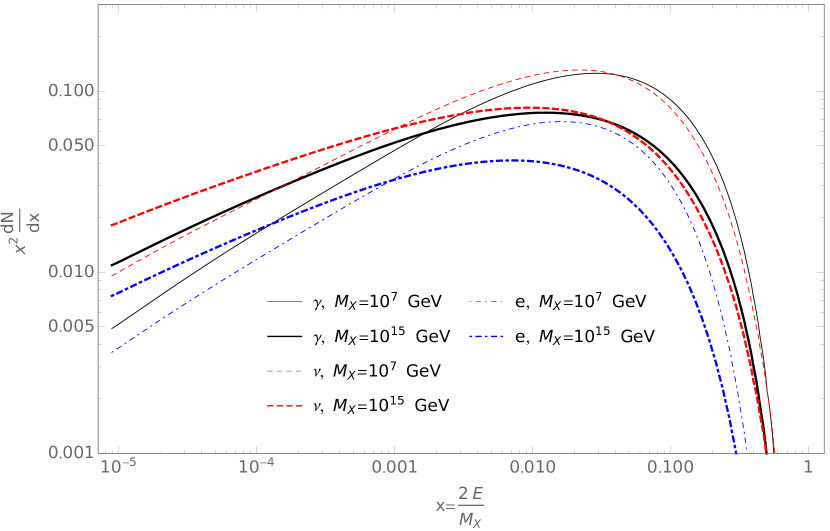
(a) $X\rightarrow q\bar{q}$

(b) $X\rightarrow\nu\bar{\nu}$

Figure 1: Prompt spectra of $X$-particle decay for the hadronic channel (left panel) and the leptonic channel (right panel) into photons (solid lines), neutrinos (dashed lines) and electrons (dot-dashed lines). For each channel, the spectra are shown for two values of the mass: $M_{X}=10^{7}$ GeV (thin lines) and $M_{X}=10^{15}$ GeV (thick lines).

3 Source distribution and high-energy particles propagation

It is convenient to consider separately the flux from dark matter (DM) decays in the Milky Way and the extragalactic flux from the entire Universe. In this work we use flux predictions for photons with energies above 100 TeV to build the constraints. The attenuation length of photons with such energies is small enough to neglect their extragalactic contribution (see e.g. Fig. 7 of Ref. [64]). For the neutrino flux, the contribution of individual distant sources is negligible, but the total extragalactic flux is sizable because neutrinos propagate over cosmological distances unattenuated. The Galactic part of the DM decay neutrino flux is described by the following expression:

$$\frac{dN^{\rm G}}{dE}\left(E\right)=\frac{1}{4\pi\tau M_{X}}\;\int\limits_{V}\frac{\rho_{{\rm DM}}\left(R[r]\right)}{4\pi r^{2}}\frac{dN}{dE}(E,l,b)\;dV\;,$$ (4)

where $\rho_{DM}\left(R\right)$ is the DM density as a function of the distance $R$ from the Galactic center, $r$ is the distance from the Earth, $l$ and $b$ are galactic coordinates and $\frac{dN}{dE}(E,l,b)$ is the spectrum of neutrinos per decaying $X$ particle. The integration is taken over all the volume of the Milky Way halo, for which we assume $R_{\max}=260$ kpc. We use the Navarro-Frenk-White (NFW) profile for the dark matter density [65, 66]  with the parametrization for the Milky Way from Ref. [57].

The evaluation of the isotropic extragalactic neutrino flux takes into account the cosmological redshift:

$$\frac{dN^{\rm EG}}{dE}\left(E_{\nu}\right)=\frac{1}{4\pi M_{X}\tau}\int\limits_{0}^{\infty}\frac{\rho_{0}\,c/H_{0}}{\sqrt{\Omega_{m}(1+z)^{3}+(1-\Omega_{m})}}\frac{dN}{dE}\left[E(1+z)\right]dz$$ (5)

where $c/H_{0}=1.37\cdot 10^{28}$ cm is the Hubble radius, $\rho_{0}=1.15\cdot 10^{-6}\;{\rm GeV}/{\rm cm}^{3}$ is the present average cosmological dark matter density, $\Omega_{m}=0.308$ and the injected spectrum $\frac{dN}{dE}$ is evaluated as a function of the particle energy at redshift $z$, $E(z)=(1+z)E$. For neutrinos, the injected flavor composition is also modified by oscillations during their propagation. We assume that the flux reaching the Earth is completely mixed, i.e. that the flavor ratio $\nu_{e}:\nu_{\mu}:\nu_{\tau}$ equals $1:1:1$.

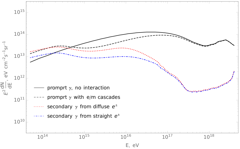
(a) $X\rightarrow\nu\bar{\nu}$

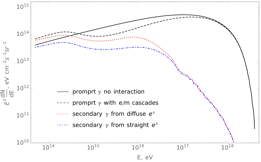
(b) $X\rightarrow q\bar{q}$

(c) $X\rightarrow\nu\bar{\nu}$

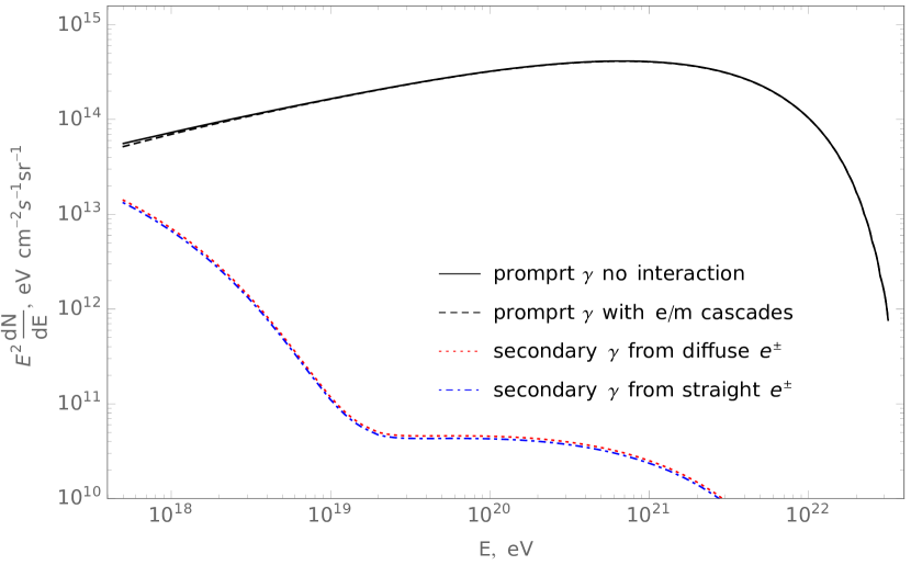
(d) $X\rightarrow q\bar{q}$

Figure 2: Comparison of prompt (noninteracting and with account of the electromagnetic cascades) and secondary (for the assumptions of straight and diffuse propagation of $e^{\pm}$) photon flux from DM decays with mass $M_{X}=10^{10}$ GeV (top) and $M_{X}=10^{14}$ GeV (bottom) in the Milky Way halo (corresponding to the exposure of the Telescope Array experiment). The magnetic field is assumed to be $B_{\rm halo}=10^{-7}$G.

To calculate the photon flux one has to take into account attenuation effects. $e^{\pm}$ produced in X-particle decays rapidly loose their energy via synchrotron losses and up-scattering CMB photons. Both processes contribute to the observable secondary $\gamma$-ray flux. The $\gamma$-rays with energies above few hundred TeV may in turn produce $e^{\pm}$ pairs on CMB photons on a scale of tens of kpc. We take these effects into account by calculating the flux from pointlike volumes inside the halo using the numerical code [68, 64] and weighting the contributions of different volumes according to Eq. (4). The numerical code simulates the development of electron-photon cascades on the CMB driven by the chain of $e^{\pm}$ pair production and inverse Compton scattering. While the code allows to calculate the flux of the cascade and synchrotron photons, it does not take into account deflections of $e^{\pm}$ by the magnetic field in the Galactic halo. Since electrons in the code propagate rectilinearly, they produce less cascade photons. Therefore, the flux of photons calculated in this approximation should be considered as a conservative lower bound. For the case of $e^{\pm}$ decay products an opposite approximation is often used (see e.g. Ref. [57]). Namely, one assumes that electrons are kept by magnetic fields in the region of their production until they loose all their energy via synchrotron or inverse Compton up-scattering of CMB photons. The secondary gamma rays then propagate towards the observer rectilinearly. We calculate the secondary $\gamma$-ray flux in both of these approximations, which we call below straight and diffusive, correspondingly. We can estimate the relevance of these two approximations as follows: Electrons with energy $E=10^{15}$ eV have a Larmor radius $R_{L}\simeq 100$ pc in a magnetic field of strength $B=0.1\mu$G. Assuming that the turbulent field has a coherence length of order $100$ pc, electrons with smaller energy diffuse in the large-angle scattering regime. Then the energy-loss time due to synchrotron radiation is at all energies of interest smaller than the escape time from an extended magnetic halo of size $\sim 50$ kpc.

The prompt and the secondary photon fluxes obtained in both approximations are compared with the prompt flux calculated without attenuation effects in Fig. 2. One should note that for the hadronic decay channel the secondary $\gamma$-ray flux is subdominant for both high and low $M_{X}$: it starts to dominate only at the low $x$ part of the energy spectra for $M_{X}\gtrsim 10^{15}$ GeV due to synchrotron emission. Therefore the impact of the secondary $\gamma$-ray on the HDM constraints is negligible for the $X\rightarrow q\bar{q}$ channel if $M_{X}\lesssim 10^{15}$ GeV.

Besides the $e^{\pm}$ propagation regime, the secondary gamma-ray flux also depends significantly on the value of the magnetic field in the Milky Way halo. Both the strength and the structure of this field are rather uncertain, but, e.g., in the simulations of Ref. [69] the field strength is of the order $B\simeq 10^{-7}$G at 50 kpc distance from the center of Milky Way-like galaxies. To account for these uncertainties, we consider as two representative cases the constant values $B=10^{-7}$G and $B=3\cdot 10^{-7}$G for the magnetic field strength disregarding its possible dependence on distance from center. We compare the propagated prompt and secondary spectra for the above cases and two values of the DM mass in Fig. 3.

(a) $M_{X}=10^{7}$ GeV, diffuse $e^{\pm}$ propagation

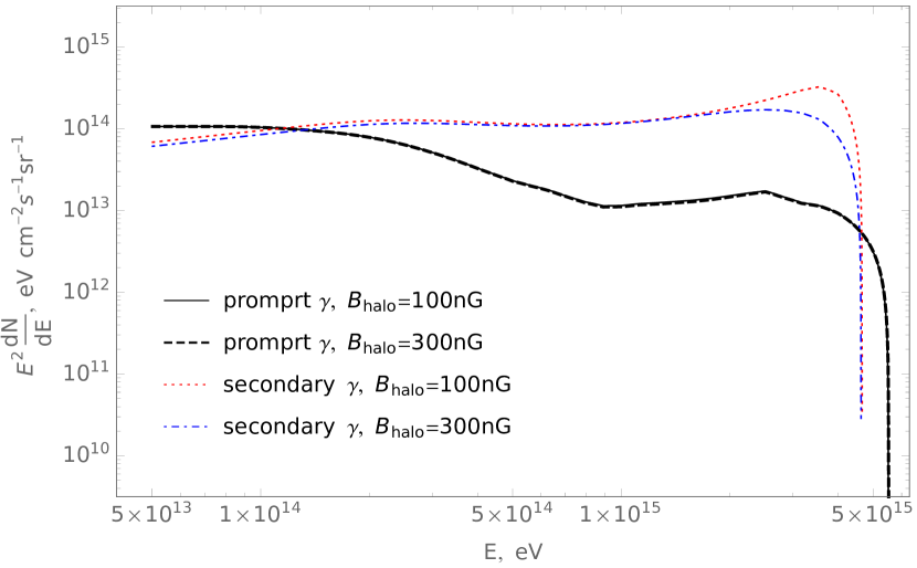
(b) $M_{X}=10^{7}$ GeV, straight $e^{\pm}$ propagation

(c) $M_{X}=10^{14}$ GeV

Figure 3: Comparison of the prompt and secondary photon fluxes from $X\rightarrow\nu\bar{\nu}$ decays in the Milky Way halo calculated for two values of galactic halo magnetic field: $B_{\rm halo}=10^{-7}$G and $B_{\rm halo}=3\cdot 10^{-7}$G. The spectra for $M_{X}=10^{7}$ GeV are shown for the assumption of diffuse (top left) and straight (top right) propagation of prompt $e^{\pm}$. The spectra for $M_{X}=10^{14}$ GeV (bottom) are independent of $e^{\pm}$ propagation assumption. All spectra are corresponding to the exposure of the Telescope Array experiment (see Sec. 4 for details).

Since the Galactic flux is anisotropic due to the Sun’s position in the Galaxy and propagation effects, the flux prediction for a specific experiment has to be convolved with its exposure.

4 Constraints on HDM parameters

In this study we assume that the whole high-energy gamma-ray and neutrino flux is saturated by HDM decays. The procedure of building model constraints is somewhat different for gamma-ray and neutrino data. The gamma-ray exposure of EAS observatories has a universal angular dependence for all gamma-ray energies (since high energy gamma rays always produce an EAS in the atmosphere). Therefore the experimental gamma-ray results are given in the form of flux limits averaged over the experiment field-of-view (FOV). For the neutrino experiments, the exposure as a function of energy varies for different angular regions; therefore, the data are given as the number of observed events.

4.1 Gamma-ray constraints

We first discuss the gamma-ray limits and constraints. To compare the simulated photon flux with observations we need to convolve it with the exposure of the given experiment. For EAS experiments with 100% duty cycle the effective exposure is uniform over right ascension and sidereal time and can therefore be averaged over these variables. The relative exposure is given by [70]:

$$\omega(a_{0},\delta,\theta_{\text{max}})\sim(\cos a_{0}\,\cos\delta\,\sin\alpha_{m}+\alpha_{m}\sin a_{0}\,\sin\delta),$$ (6)

where $\delta$ is the declination, $a_{0}$ is the geographical latitude of the experiment, $\theta_{max}$ is the maximum photon search zenith angle in the experiment and $\alpha_{m}$ is given by

$$\alpha_{m}=\begin{cases}0&;\xi>1,\\ \pi&;\xi<-1,\\ \arccos\xi&;-1<\xi<1\,;\end{cases}$$ (7)

$$\xi=\frac{(\cos\theta_{\text{max}}-\sin a_{0}\,\sin\delta)}{\cos a_{0}\,\cos\delta}.$$ (8)

There is no need to know the overall normalization of the exposure, since experimental results are given as a flux limit differential over time, area and FOV. In the class of 100% duty cycle EAS experiments the most recent results are given by the Pierre Auger surface detectors [71], the Telescope Array surface detectors [72], Yakutsk [73], EAS-MSU [74], KASCADE and KASCADE-Grande experiments [75]. We also use the results of the CASA-MIA experiment [76]. It is worth noting that some of KASCADE and KASCADE-Grande’s recent limits are somewhat less strict than their previous results. Therefore one expects weaker HDM-lifetime constraints. There are also strong limits provided by the Pierre Auger experiment in the hybrid mode [77], in which duty cycle is however not 100% and its exposure is nonuniform over right ascension and sidereal time. Since there is no publicly available description of the exposure dependence on sidereal time we use the same formula (6) for the Auger hybrid exposure implying the respective HDM constraint is a rough overestimation of the real one.

The integral photon flux received by a given EAS observatory is expressed as:

$$F(E>E_{min})=\frac{1}{4\pi M_{X}\tau_{X}}\frac{\int\limits_{E_{\min}}^{\infty}\int\limits_{V}\frac{\rho(R)\omega(l,b,a_{0},\theta_{\max})}{r^{2}}\frac{dN}{dE}(E,l,b)dVdE}{2\pi\int\limits_{-\frac{\pi}{2}}^{\frac{\pi}{2}}\omega(\delta,a_{0},\theta_{\max})\cos(\delta)d\delta}\;;$$ (9)

where $\rho(R)$ is the DM density as a function of the distance $R$ from the Galactic center, $r$ is the distance from the Earth, $l$ and $b$ are Galactic coordinates and $\frac{dN}{dE}(E,l,b)$ is the spectrum of primary and secondary photons produced per decaying $X$ particle. The integration in the numerator is taken over all the volume of the DM halo ($R_{\max}=260$ kpc) and in the denominator over all sky (the cut of the unseen sky regions is included into the definition of $\omega$).

Given the predicted gamma-ray flux observable by the particular experiment we obtain the minimal DM lifetime by varying it until the flux matches at least one of the experimental limits. Separate constraints for $X\rightarrow q\bar{q}$ and $X\rightarrow\nu\bar{\nu}$ ($X\rightarrow e^{+}e^{-}$) decay channels are shown in Fig. 4. For both channels the most strict constraints are given by the Pierre Auger Observatory, KASCADE-Grande, KASCADE and CASA-MIA. For each channel we show the constraints for two distinct cases of secondary photon flux calculation discussed in Sec. 3: quasistraight propagation of $e^{\pm}$ and its diffusion until the complete emission of energy into photons. One can see that these two cases produce similar constraints starting from $M_{X}\gtrsim 5\cdot 10^{9}$ GeV.

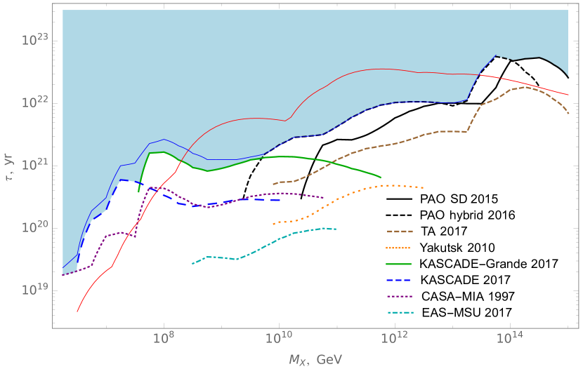
(a) $\gamma$-constraints

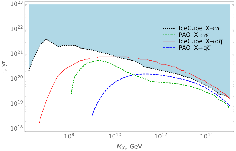
(b) $\nu$-constraints

Figure 4: Constraints on the parameters of HDM for the $X\rightarrow\nu\bar{\nu}$ decay channel derived from various experimental gamma-ray limits (left panel) and neutrino data (right panel). The white area is excluded. The gamma constraints shown assume secondary gamma rays from quasistraight propagation of $e^{\pm}$ in Galaxy (white area) or diffuse $e^{\pm}$ propagation (below solid blue line). The all-experiments constraint from both gamma ray and neutrino for the $X\rightarrow q\bar{q}$ decay channel is shown by the solid red line. For neutrino data, the constraints are at 90% C.L. For gamma-ray data, the KASCADE, CASA-MIA, KASCADE-Grande and EAS-MSU constraints are at 90% C.L.; the Yakutsk, Pierre Auger and Telescope Array constraints are at 95% C.L.

4.2 Neutrino constraints

In this work we use the neutrino observations by IceCube [5], recently updated in Ref. [6] (Sec. 9). This data set contains two events with 2.6 PeV and 2.7 PeV energies, we assume that they have HDM origin. For comparison, we also use the results of neutrino nonobservation by Pierre Auger [78].

We build HDM constraints with the neutrino data using the procedure discussed in detail in Ref. [19]. Namely, we compare the observed number of neutrino events with the number predicted by the model assuming the exposure of the particular experiment [79]. For the Galactic neutrino flux the calculation yields:

$$N_{\rm G}^{\nu}=\frac{1}{4\pi M_{X}\tau}\int\limits_{\Delta E}\int\limits_{V}\rho\left[R(r,\delta,\alpha)\right]\>\omega(E,\delta,\alpha)\>\frac{dN}{dE}(E)\>\cos(\delta)\>dr\>d\delta\>d\alpha\>dE\;,$$ (10)

where the integration is performed over all the volume of the dark-matter halo ($R<260$ kpc) and over the neutrino energy range $\Delta E$ accessible by a given experiment. In practice, the exposure is given for several zenith angle bands, averaged over each band. For IceCube we adopt the exposure as a function of declination (which uniquely translates to zenith angle in the case of IceCube) and energy as it is given in Ref. [80] and normalize it to the actual IceCube exposure of Ref. [5]. For the Pierre Auger Observatory we use the exposure given in Ref. [78].

The number of events from the extragalactic neutrino flux is

$$N_{\rm EG}=\int\limits_{\Delta E}\omega(E)\>\frac{dN_{\rm EG}}{dE}(E)\>dE\;,$$ (11)

where the exposure $\varepsilon(E)$ is integrated over the celestial sphere. The total number of events predicted by the model is

$$N_{\rm th}=N_{\rm G}+N_{\rm EG}\,.$$ (12)

For each mass $M_{X}$ we constrain the lifetime $\tau$ according to the binned Poisson Monte Carlo procedure described in Ref. [19]. Namely, we generate many Monte–Carlo sets with the number of events in each energy bin, $N_{\rm MC}^{i}$, following a Poisson distribution with mean $\lambda^{i}=N_{\rm th}^{i}$, which equals the expected average number of events for a given $\tau$ and $M_{X}$. The minimal allowed value of $\tau$ is the value for which the fraction of Monte Carlo sets with $N_{\rm MC}^{i}>N_{\rm obs}^{i}$ in at least one bin reaches the given confidence level. The method is applicable when the number of background events is negligible, which is true for the discussed IceCube data set [5]. The constraints on the parameter space $\{M_{X},\tau\}$ are presented in Fig. 4.

5 Discussion

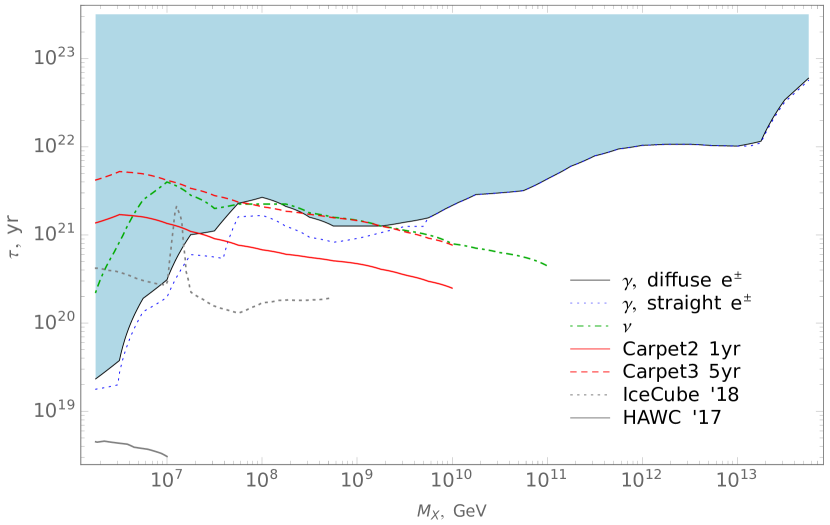
(a) $X\rightarrow\nu\bar{\nu}$

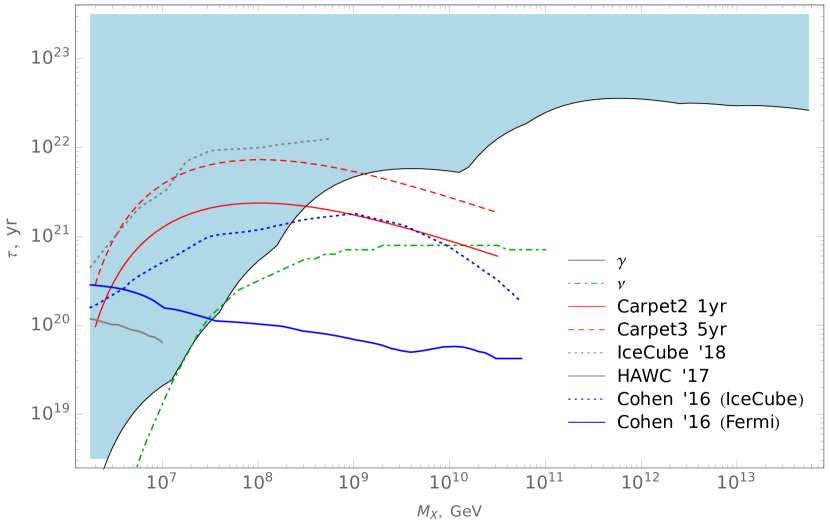
(b) $X\rightarrow q\bar{q}$

Figure 5: Gamma ray vs. neutrino constraints on HDM parameters for leptonic decay (left panel) and hadronic decay channels (right panel). For the leptonic decay, the constraints with secondary gamma rays from straight $e^{\pm}$ (blue dashed line) and diffuse $e^{\pm}$ (black solid line) are shown. For both decay channels, the prospective constraints for diffuse gamma-ray searches of the Carpet experiment [81] are shown for 1 year of Carpet2 observations (solid red line) and 5 years of Carpet3 observations (dashed red line). The constraints for $X\rightarrow\nu\bar{\nu}$ channel from Refs. [48, 45] and for the $X\rightarrow b\bar{b}$ channel from Refs. [48, 15, 45] are shown for comparison on the left panel and right panel, respectively.

We have studied the hypothesis of heavy dark matter particles $X$ of mass $10^{6}\leq M_{X}\leq\leavevmode\nobreak\ 10^{16}$ GeV decaying on tree level into $X\rightarrow\nu\bar{\nu}$, $X\rightarrow e^{+}e^{-}$ and $X\rightarrow q\bar{q}$ in the context of the IceCube highest energy neutrino events and recent limits on the diffuse flux of high-energy photons. For neutrino flux constraints we have selected the data set [5, 6] among the various IceCube measurements as the most conservative one. The analysis cuts for this set are relatively strict, aiming at eliminating all atmospheric neutrino backgrounds. This should lead, of course, to a reduction in the total neutrino exposure, but two events with 2.6 PeV and 2.7 PeV energies in the resulting neutrino set are found to be consistent with astrophysical neutrino comparing to Monte Carlo simulations. In this study we assume that these events are of HDM decay origin, which does not contradict the mentioned IceCube studies. There are several works [15, 16, 17] that use other IceCube data sets [82, 6] to constrain the HDM parameters, as well as the recent work on HDM search by the IceCube collaboration itself [48]. These studies set HDM constraints employing a likelihood analysis of the neutrino spectrum, assuming an arbitrary combination of neutrinos with astrophysical and HDM decay origin in a wide energy range. The larger exposure of the data sets and the complexity of the fit models used in these studies results in quite strong constraints on HDM parameters. In contrast, the constraints derived in this work with a relatively simple approach are more conservative.

A comparison of gamma ray and neutrino constraints for the $X\leavevmode\nobreak\ \rightarrow\leavevmode\nobreak\ \nu\bar{\nu}$ and $X\leavevmode\nobreak\ \rightarrow\leavevmode\nobreak\ q\bar{q}$ decay channels is shown in Fig. 5 together with some $\gamma$-ray and neutrino constraints from other studies. One should note that for hadronically decaying HDM the neutrino constraints obtained in this work are weaker than the gamma-ray ones for almost the entire mass range considered. This implies that hadronically decaying HDM as an explanation of the highest energies IceCube events is disfavored. For the leptonic decay channel the situation is the opposite: the IceCube high energy signal could be explained by HDM with masses up to $M_{X}\leavevmode\nobreak\ \lesssim\leavevmode\nobreak\ 5.5\cdot 10^{7}$ GeV and $\leavevmode\nobreak\ 1.5\cdot 10^{8}\leavevmode\nobreak\ \lesssim M_{X}\leavevmode\nobreak\ \lesssim\leavevmode\nobreak\ 1.5\cdot 10^{9}$ GeV.

The part of parameter space allowed by the current $\gamma$-ray limits can be further constrained with ongoing and future high-energy gamma experiments. For instance the Carpet EAS experiment of the Baksan Neutrino Observatory is currently operating and undergoing consecutive upgrades to an area of 410 m² (Carpet2) and 615 m² (Carpet3). After the later upgrade it will be sensitive to $\gamma$-rays in the energy range from 100 TeV to 30 PeV, with more than an order of magnitude increased sensitivity at 100 TeV compared to the current KASCADE limit [81]. In Fig. 5 we illustrate the range of model parameters which can be excluded by the Carpet experiment, if the $\gamma$-ray flux is not detected. One can see that the experiment will be capable to cover a significant part of the remaining open parameter space of models explaining the IceCube neutrino flux within one year of observation. It is able to close this window practically within five years of observation after the second upgrade.

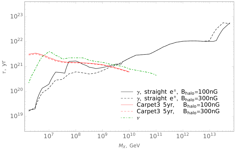
(a) Straight $e^{\pm}$ propagation

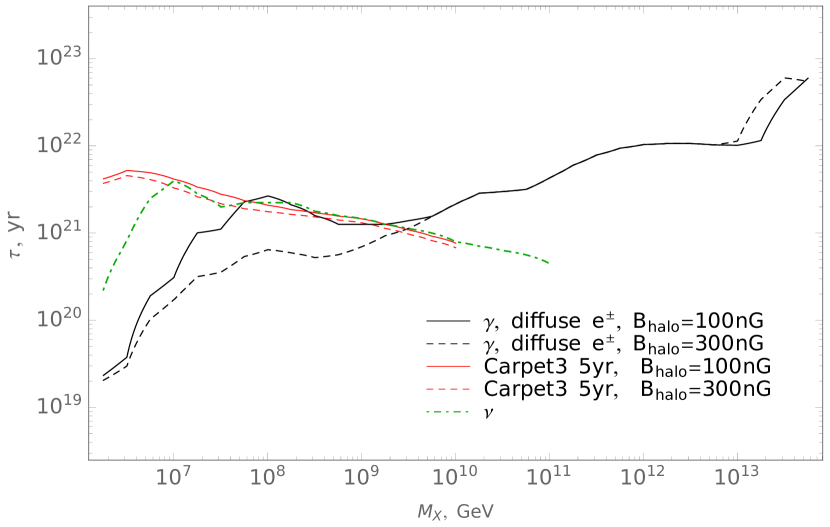
(b) Diffuse $e^{\pm}$ propagation

Figure 6: Gamma-ray vs. neutrino constraints on HDM parameters for leptonic decay: comparison of $B_{\rm halo}=10^{-7}$G and $B_{\rm halo}=3\cdot 10^{-7}$G cases for straight (left panel) and diffuse (right panel) propagation of electrons. In both cases the prospective constraints for diffuse gamma-ray searches of the Carpet experiment [81] are also shown by red lines.

However, the constraint obtained for the $X\leavevmode\nobreak\ \rightarrow\leavevmode\nobreak\ \nu\bar{\nu}$ channel is dependent on the assumed value of the halo magnetic field. We compare the limits derived using the field strength values $B_{\rm halo}=10^{-7}$G and $B_{h\rm alo}=3\cdot 10^{-7}$G in Fig. 6: For higher magnetic field strength the flux of secondary photons is suppressed and the constraint weakens. We should also stress that in the case of $X\leavevmode\nobreak\ \rightarrow\leavevmode\nobreak\ q\bar{q}$ channel the limits are not affected by the strength of the magnetic field, since the contribution of the secondary gamma rays to the total gamma-ray flux is negligible for this channel.

References

- [1] M. G. Aartsen et al. Evidence for High-Energy Extraterrestrial Neutrinos at the IceCube Detector. Science, 342:1242856, 2013. arXiv:1311.5238, doi:10.1126/science.1242856.
- [2] M. G. Aartsen et al. Observation of High-Energy Astrophysical Neutrinos in Three Years of IceCube Data. Phys. Rev. Lett., 113:101101, 2014. arXiv:1405.5303, doi:10.1103/PhysRevLett.113.101101.
- [3] M. Ahlers and F. Halzen. IceCube: Neutrinos and multimessenger astronomy. Progress of Theoretical and Experimental Physics, 2017(12):12A105, December 2017. doi:10.1093/ptep/ptx021.
- [4] A. Neronov, M. Kachelrieß, and D. V. Semikoz. Discovery of the multi-messenger gamma-ray counterpart of the IceCube neutrino signal. 2018. arXiv:1802.09983.
- [5] M. G. Aartsen et al. Constraints on Ultrahigh-Energy Cosmic-Ray Sources from a Search for Neutrinos above 10 PeV with IceCube. Phys. Rev. Lett., 117(24):241101, 2016. [Erratum: Phys. Rev. Lett.119,no.25,259902(2017)]. arXiv:1607.05886, doi:10.1103/PhysRevLett.117.241101,10.1103/PhysRevLett.119.259902,10.1103/PhysRevLett.117.241101,10.1103/PhysRevLett.119.259902.
- [6] M. G. Aartsen et al. The IceCube Neutrino Observatory - Contributions to ICRC 2017 Part II: Properties of the Atmospheric and Astrophysical Neutrino Flux. 2017. arXiv:1710.01191.
- [7] V. Berezinsky, M. Kachelrieß, and A. Vilenkin. Ultrahigh-energy cosmic rays without GZK cutoff. Phys. Rev. Lett., 79:4302–4305, 1997. arXiv:astro-ph/9708217, doi:10.1103/PhysRevLett.79.4302.
- [8] Brian Feldstein, Alexander Kusenko, Shigeki Matsumoto, and Tsutomu T. Yanagida. Neutrinos at IceCube from Heavy Decaying Dark Matter. Phys. Rev., D88(1):015004, 2013. arXiv:1303.7320, doi:10.1103/PhysRevD.88.015004.
- [9] Arman Esmaili and Pasquale Dario Serpico. Are IceCube neutrinos unveiling PeV-scale decaying dark matter? JCAP, 1311:054, 2013. arXiv:1308.1105, doi:10.1088/1475-7516/2013/11/054.
- [10] Atri Bhattacharya, Mary Hall Reno, and Ina Sarcevic. Reconciling neutrino flux from heavy dark matter decay and recent events at IceCube. JHEP, 06:110, 2014. arXiv:1403.1862, doi:10.1007/JHEP06(2014)110.
- [11] Carsten Rott, Kazunori Kohri, and Seong Chan Park. Superheavy dark matter and IceCube neutrino signals: Bounds on decaying dark matter. Phys. Rev., D92(2):023529, 2015. arXiv:1408.4575, doi:10.1103/PhysRevD.92.023529.
- [12] Arman Esmaili, Sin Kyu Kang, and Pasquale Dario Serpico. IceCube events and decaying dark matter: hints and constraints. JCAP, 1412(12):054, 2014. arXiv:1410.5979, doi:10.1088/1475-7516/2014/12/054.
- [13] Kohta Murase, Ranjan Laha, Shin’ichiro Ando, and Markus Ahlers. Testing the Dark Matter Scenario for PeV Neutrinos Observed in IceCube. Phys. Rev. Lett., 115(7):071301, 2015. arXiv:1503.04663, doi:10.1103/PhysRevLett.115.071301.
- [14] P. S. Bhupal Dev, D. Kazanas, R. N. Mohapatra, V. L. Teplitz, and Yongchao Zhang. Heavy right-handed neutrino dark matter and PeV neutrinos at IceCube. JCAP, 1608(08):034, 2016. arXiv:1606.04517, doi:10.1088/1475-7516/2016/08/034.
- [15] Timothy Cohen, Kohta Murase, Nicholas L. Rodd, Benjamin R. Safdi, and Yotam Soreq. Gamma-ray Constraints on Decaying Dark Matter and Implications for IceCube. Phys. Rev. Lett., 119(2):021102, 2017. arXiv:1612.05638, doi:10.1103/PhysRevLett.119.021102.
- [16] Yicong Sui and P. S. Bhupal Dev. A Combined Astrophysical and Dark Matter Interpretation of the IceCube HESE and Throughgoing Muon Events. 2018. arXiv:1804.04919.
- [17] Atri Bhattacharya, Arman Esmaili, Sergio Palomares-Ruiz, and Ina Sarcevic. Probing decaying heavy dark matter with the 4-year IceCube HESE data. JCAP, 1707(07):027, 2017. arXiv:1706.05746, doi:10.1088/1475-7516/2017/07/027.
- [18] Debasish Borah, Arnab Dasgupta, Ujjal Kumar Dey, Sudhanwa Patra, and Gaurav Tomar. Multi-component Fermionic Dark Matter and IceCube PeV scale Neutrinos in Left-Right Model with Gauge Unification. JHEP, 09:005, 2017. arXiv:1704.04138, doi:10.1007/JHEP09(2017)005.
- [19] M. Yu. Kuznetsov. Hadronically decaying heavy dark matter and high-energy neutrino limits. JETP Lett., 105(9):561–567, 2017. arXiv:1611.08684, doi:10.1134/S0021364017090028.
- [20] Ya. B. Zeldovich and Alexei A. Starobinsky. Particle production and vacuum polarization in an anisotropic gravitational field. Sov. Phys. JETP, 34:1159–1166, 1972. [Zh. Eksp. Teor. Fiz.61,2161(1971)].
- [21] Ya. B. Zeldovich and A. A. Starobinsky. Rate of particle production in gravitational fields. JETP Lett., 26:252–255, 1977. [Zh. Eksp. Teor. Fiz.26,373(1977)].
- [22] Lev Kofman, Andrei D. Linde, and Alexei A. Starobinsky. Reheating after inflation. Phys. Rev. Lett., 73:3195–3198, 1994. arXiv:hep-th/9405187, doi:10.1103/PhysRevLett.73.3195.
- [23] S. Yu. Khlebnikov and I. I. Tkachev. Resonant decay of Bose condensates. Phys. Rev. Lett., 79:1607–1610, 1997. arXiv:hep-ph/9610477, doi:10.1103/PhysRevLett.79.1607.
- [24] S. Yu. Khlebnikov and I. I. Tkachev. The Universe after inflation: The Wide resonance case. Phys. Lett., B390:80–86, 1997. arXiv:hep-ph/9608458, doi:10.1016/S0370-2693(96)01419-0.
- [25] V. A. Kuzmin and V. A. Rubakov. Ultrahigh-energy cosmic rays: A Window to postinflationary reheating epoch of the universe? Phys. Atom. Nucl., 61:1028, 1998. arXiv:astro-ph/9709187.
- [26] Vadim Kuzmin and Igor Tkachev. Matter creation via vacuum fluctuations in the early universe and observed ultrahigh-energy cosmic ray events. Phys. Rev., D59:123006, 1999. arXiv:hep-ph/9809547, doi:10.1103/PhysRevD.59.123006.
- [27] Daniel J. H. Chung, Edward W. Kolb, and Antonio Riotto. Production of massive particles during reheating. Phys. Rev., D60:063504, 1999. arXiv:hep-ph/9809453, doi:10.1103/PhysRevD.60.063504.
- [28] Daniel J. H. Chung, Edward W. Kolb, and Antonio Riotto. Superheavy dark matter. Phys. Rev., D59:023501, 1999. arXiv:hep-ph/9802238, doi:10.1103/PhysRevD.59.023501.
- [29] Vadim Kuzmin and Igor Tkachev. Ultrahigh-energy cosmic rays, superheavy long living particles, and matter creation after inflation. JETP Lett., 68:271–275, 1998. [Pisma Zh. Eksp. Teor. Fiz.68,255(1998)]. arXiv:hep-ph/9802304, doi:10.1134/1.567858.
- [30] M. Yu. Khlopov and V. M. Chechetkin. Anti-protons in the Universe as Cosmological Test of Grand Unification. (In Russian). Fiz. Elem. Chast. Atom. Yadra, 18:627–677, 1987.
- [31] Daniele Fargion, M. Yu. Khlopov, R. V. Konoplich, V. R. Konoplich, and R. Mignani. On the possibility of detecting the annihilation of very heavy neutrinos in the galactic halo by 1-km**3 neutrino detector. Mod. Phys. Lett., A11:1363–1370, 1996. doi:10.1142/S0217732396001375.
- [32] Paolo Gondolo, Graciela Gelmini, and Subir Sarkar. Cosmic neutrinos from unstable relic particles. Nucl. Phys., B392:111–136, 1993. arXiv:hep-ph/9209236, doi:10.1016/0550-3213(93)90199-Y.
- [33] Edward W. Kolb, Daniel J. H. Chung, and Antonio Riotto. WIMPzillas! In Trends in theoretical physics II. Proceedings, 2nd La Plata Meeting, Buenos Aires, Argentina, November 29-December 4, 1998, pages 91–105, 1998. [,91(1998)]. URL: http://lss.fnal.gov/cgi-bin/find_paper.pl?conf-98-325, arXiv:hep-ph/9810361.
- [34] Vadim A. Kuzmin and Igor I. Tkachev. Ultrahigh-energy cosmic rays and inflation relics. Phys. Rept., 320:199–221, 1999. arXiv:hep-ph/9903542, doi:10.1016/S0370-1573(99)00064-2.
- [35] Daniel J. H. Chung, Edward W. Kolb, Antonio Riotto, and Leonardo Senatore. Isocurvature constraints on gravitationally produced superheavy dark matter. Phys. Rev., D72:023511, 2005. arXiv:astro-ph/0411468, doi:10.1103/PhysRevD.72.023511.
- [36] D. S. Gorbunov and A. G. Panin. Free scalar dark matter candidates in -inflation: the light, the heavy and the superheavy. Phys. Lett., B718:15–20, 2012. arXiv:1201.3539, doi:10.1016/j.physletb.2012.10.015.
- [37] Kim Griest and Marc Kamionkowski. Unitarity Limits on the Mass and Radius of Dark Matter Particles. Phys. Rev. Lett., 64:615, 1990. doi:10.1103/PhysRevLett.64.615.
- [38] Oleg E. Kalashev, G. I. Rubtsov, and Sergey V. Troitsky. Sensitivity of cosmic-ray experiments to ultra-high-energy photons: reconstruction of the spectrum and limits on the superheavy dark matter. Phys. Rev., D80:103006, 2009. arXiv:0812.1020, doi:10.1103/PhysRevD.80.103006.
- [39] O. E. Kalashev and M. Yu Kuznetsov. Heavy decaying dark matter and large-scale anisotropy of high-energy cosmic rays. JETP Lett., 106(2):73–80, 2017. [Pisma Zh. Eksp. Teor. Fiz.106,no.2,65(2017)]. arXiv:1704.05300, doi:10.1134/S0021364017140016.
- [40] Luca Marzola and Federico R Urban. Ultra High Energy Cosmic Rays & Super-heavy Dark Matter. Astropart. Phys., 93:56–69, 2017. arXiv:1611.07180, doi:10.1016/j.astropartphys.2017.04.005.
- [41] Kohta Murase and John F. Beacom. Constraining Very Heavy Dark Matter Using Diffuse Backgrounds of Neutrinos and Cascaded Gamma Rays. JCAP, 1210:043, 2012. arXiv:1206.2595, doi:10.1088/1475-7516/2012/10/043.
- [42] R. Aloisio, S. Matarrese, and A. V. Olinto. Super Heavy Dark Matter in light of BICEP2, Planck and Ultra High Energy Cosmic Rays Observations. JCAP, 1508(08):024, 2015. arXiv:1504.01319, doi:10.1088/1475-7516/2015/08/024.
- [43] Arman Esmaili and Pasquale Dario Serpico. Gamma-ray bounds from EAS detectors and heavy decaying dark matter constraints. JCAP, 1510(10):014, 2015. arXiv:1505.06486, doi:10.1088/1475-7516/2015/10/014.
- [44] O. K. Kalashev and M. Yu. Kuznetsov. Constraining heavy decaying dark matter with the high energy gamma-ray limits. Phys. Rev., D94(6):063535, 2016. arXiv:1606.07354, doi:10.1103/PhysRevD.94.063535.
- [45] A. U. Abeysekara et al. A Search for Dark Matter in the Galactic Halo with HAWC. JCAP, 1802(02):049, 2018. arXiv:1710.10288, doi:10.1088/1475-7516/2018/02/049.
- [46] R. Abbasi et al. Search for dark matter from the Galactic halo with the IceCube Neutrino Telescope. Phys. Rev., D84:022004, 2011. arXiv:1101.3349, doi:10.1103/PhysRevD.84.022004.
- [47] Arman Esmaili, Alejandro Ibarra, and Orlando L. G. Peres. Probing the stability of superheavy dark matter particles with high-energy neutrinos. JCAP, 1211:034, 2012. arXiv:1205.5281, doi:10.1088/1475-7516/2012/11/034.
- [48] M. G. Aartsen et al. Search for neutrinos from decaying dark matter with IceCube. 2018. arXiv:1804.03848.
- [49] V. Berezinsky and M. Kachelrieß. Ultrahigh-energy LSP. Phys. Lett., B422:163–170, 1998. arXiv:hep-ph/9709485, doi:10.1016/S0370-2693(98)00068-9.
- [50] V. Berezinsky and M. Kachelrieß. New particles as ultrahigh-energy primaries. Nucl. Phys. Proc. Suppl., 75A:377–379, 1999. doi:10.1016/S0920-5632(99)00297-2.
- [51] V. Berezinsky and M. Kachelrieß. Monte Carlo simulation for jet fragmentation in SUSY QCD. Phys. Rev., D63:034007, 2001. arXiv:hep-ph/0009053, doi:10.1103/PhysRevD.63.034007.
- [52] R. Aloisio, V. Berezinsky, and M. Kachelrieß. Fragmentation functions in SUSY QCD and UHECR spectra produced in top - down models. Phys. Rev., D69:094023, 2004. arXiv:hep-ph/0307279, doi:10.1103/PhysRevD.69.094023.
- [53] V. Berezinsky and M. Kachelrieß. Limiting SUSY QCD spectrum and its application for decays of superheavy particles. Phys. Lett., B434:61–66, 1998. arXiv:hep-ph/9803500, doi:10.1016/S0370-2693(98)00728-X.
- [54] Subir Sarkar and Ramon Toldra. The High-energy cosmic ray spectrum from relic particle decay. Nucl. Phys., B621:495–520, 2002. arXiv:hep-ph/0108098, doi:10.1016/S0550-3213(01)00565-X.
- [55] Cyrille Barbot and Manuel Drees. Production of ultraenergetic cosmic rays through the decay of superheavy X particles. Phys. Lett., B533:107–115, 2002. arXiv:hep-ph/0202072, doi:10.1016/S0370-2693(02)01621-0.
- [56] Cyrille Barbot and Manuel Drees. Detailed analysis of the decay spectrum of a super heavy X particle. Astropart. Phys., 20:5–44, 2003. arXiv:hep-ph/0211406, doi:10.1016/S0927-6505(03)00134-8.
- [57] Marco Cirelli, Gennaro Corcella, Andi Hektor, Gert Hutsi, Mario Kadastik, Paolo Panci, Martti Raidal, Filippo Sala, and Alessandro Strumia. PPPC 4 DM ID: A Poor Particle Physicist Cookbook for Dark Matter Indirect Detection. JCAP, 1103:051, 2011. [Erratum: JCAP1210,E01(2012)]. arXiv:1012.4515, doi:10.1088/1475-7516/2012/10/E01,10.1088/1475-7516/2011/03/051.
- [58] V. N. Gribov and L. N. Lipatov. e+ e- pair annihilation and deep inelastic e p scattering in perturbation theory. Sov. J. Nucl. Phys., 15:675–684, 1972. [Yad. Fiz.15,1218(1972)].
- [59] Guido Altarelli and G. Parisi. Asymptotic Freedom in Parton Language. Nucl. Phys., B126:298–318, 1977. doi:10.1016/0550-3213(77)90384-4.
- [60] Yuri L. Dokshitzer. Calculation of the Structure Functions for Deep Inelastic Scattering and e+ e- Annihilation by Perturbation Theory in Quantum Chromodynamics. Sov. Phys. JETP, 46:641–653, 1977. [Zh. Eksp. Teor. Fiz.73,1216(1977)].
- [61] M. Hirai, S. Kumano, T. H. Nagai, and K. Sudoh. Determination of fragmentation functions and their uncertainties. Phys. Rev., D75:094009, 2007. arXiv:hep-ph/0702250, doi:10.1103/PhysRevD.75.094009.
- [62] S. R. Kelner, Felex A. Aharonian, and V. V. Bugayov. Energy spectra of gamma-rays, electrons and neutrinos produced at proton-proton interactions in the very high energy regime. Phys. Rev., D74:034018, 2006. [Erratum: Phys. Rev.D79,039901(2009)]. arXiv:astro-ph/0606058, doi:10.1103/PhysRevD.74.034018,10.1103/PhysRevD.79.039901.
- [63] V. Berezinsky, M. Kachelrieß, and S. Ostapchenko. Electroweak jet cascading in the decay of superheavy particles. Phys. Rev. Lett., 89:171802, 2002. arXiv:hep-ph/0205218, doi:10.1103/PhysRevLett.89.171802.
- [64] V. Berezinsky and O. Kalashev. High energy electromagnetic cascades in extragalactic space: physics and features. Phys. Rev., D94(2):023007, 2016. arXiv:1603.03989, doi:10.1103/PhysRevD.94.023007.
- [65] Julio F. Navarro, Carlos S. Frenk, and Simon D. M. White. The Structure of cold dark matter halos. Astrophys. J., 462:563–575, 1996. arXiv:astro-ph/9508025, doi:10.1086/177173.
- [66] Julio F. Navarro, Carlos S. Frenk, and Simon D. M. White. A Universal density profile from hierarchical clustering. Astrophys. J., 490:493–508, 1997. arXiv:astro-ph/9611107, doi:10.1086/304888.
- [67] A. Burkert. The Structure of dark matter halos in dwarf galaxies. IAU Symp., 171:175, 1996. [Astrophys. J.447,L25(1995)]. arXiv:astro-ph/9504041, doi:10.1086/309560.
- [68] O. E. Kalashev and E. Kido. Simulations of Ultra High Energy Cosmic Rays propagation. J. Exp. Theor. Phys., 120(5):790–797, 2015. arXiv:1406.0735, doi:10.1134/S1063776115040056.
- [69] A. M. Beck, H. Lesch, K. Dolag, H. Kotarba, A. Geng, and F. A. Stasyszyn. Origin of strong magnetic fields in Milky Way-like galactic haloes. Mon. Not. Roy. Soc., 422:2152–2163, May 2012. arXiv:1202.3349, doi:10.1111/j.1365-2966.2012.20759.x.
- [70] P. Sommers. Cosmic ray anisotropy analysis with a full-sky observatory. Astropart. Phys., 14:271–286, 2001. arXiv:astro-ph/0004016, doi:10.1016/S0927-6505(00)00130-4.
- [71] The Pierre Auger Observatory: Contributions to the 34th International Cosmic Ray Conference (ICRC 2015), 2015. URL: http://inspirehep.net/record/1393211/files/arXiv:1509.03732.pdf, arXiv:1509.03732.
- [72] G.I. Rubtsov. Telescope Array search for EeV photons and neutrinos. PoS, ICRC2017:551, 2017.
- [73] A. V. Glushkov, I. T. Makarov, M. I. Pravdin, I. E. Sleptsov, D. S. Gorbunov, G. I. Rubtsov, and S. V. Troitsky. Constraints on the flux of primary cosmic-ray photons at energies eV from Yakutsk muon data. Phys. Rev., D82:041101, 2010. arXiv:0907.0374, doi:10.1103/PhysRevD.82.041101.
- [74] Yu. A. Fomin, N. N. Kalmykov, I. S. Karpikov, G. V. Kulikov, M. Yu Kuznetsov, G. I. Rubtsov, V. P. Sulakov, and S. V. Troitsky. Constraints on the flux of eV cosmic photons from the EAS-MSU muon data. Phys. Rev., D95(12):123011, 2017. arXiv:1702.08024, doi:10.1103/PhysRevD.95.123011.
- [75] W. D. Apel et al. KASCADE-Grande Limits on the Isotropic Diffuse Gamma-Ray Flux between 100 TeV and 1 EeV. Astrophys. J., 848(1):1, 2017. arXiv:1710.02889, doi:10.3847/1538-4357/aa8bb7.
- [76] M. C. Chantell et al. Limits on the isotropic diffuse flux of ultrahigh-energy gamma radiation. Phys. Rev. Lett., 79:1805–1808, 1997. arXiv:astro-ph/9705246, doi:10.1103/PhysRevLett.79.1805.
- [77] Alexander Aab et al. Search for photons with energies above 1018 eV using the hybrid detector of the Pierre Auger Observatory. JCAP, 1704(04):009, 2017. arXiv:1612.01517, doi:10.1088/1475-7516/2017/04/009.
- [78] Enrique Zas. Searches for neutrino fluxes in the EeV regime with the Pierre Auger Observatory. In The Pierre Auger Observatory: Contributions to the 35th International Cosmic Ray Conference (ICRC 2017), pages 64–71, 2017. URL: http://inspirehep.net/record/1618420/files/1617990_64-71.pdf.
- [79] Luis A. Anchordoqui, Jonathan L. Feng, Haim Goldberg, and Alfred D. Shapere. Neutrino bounds on astrophysical sources and new physics. Phys. Rev., D66:103002, 2002. arXiv:hep-ph/0207139, doi:10.1103/PhysRevD.66.103002.
- [80] R. Abbasi et al. Constraints on the Extremely-high Energy Cosmic Neutrino Flux with the IceCube 2008-2009 Data. Phys. Rev., D83:092003, 2011. [Erratum: Phys. Rev.D84,079902(2011)]. arXiv:1103.4250, doi:10.1103/PhysRevD.84.079902,10.1103/PhysRevD.83.092003.
- [81] D. D. Dzhappuev, V. B. Petkov, A. U. Kudzhaev, N. F. Klimenko, A. S. Lidvansky, and S. V. Troitsky. Search for cosmic gamma rays with the Carpet-2 extensive air shower array. 2015. URL: http://inspirehep.net/record/1407115/files/arXiv:1511.09397.pdf, arXiv:1511.09397.
- [82] M. G. Aartsen et al. A combined maximum-likelihood analysis of the high-energy astrophysical neutrino flux measured with IceCube. Astrophys. J., 809(1):98, 2015. arXiv:1507.03991, doi:10.1088/0004-637X/809/1/98.