The C-Band All-Sky Survey (C-BASS): Design and capabilities

Abstract

The C-Band All-Sky Survey (C-BASS) is an all-sky full-polarization survey at a frequency of 5 GHz, designed to provide complementary data to the all-sky surveys of WMAP and Planck, and future CMB $B$-mode polarization imaging surveys. The observing frequency has been chosen to provide a signal that is dominated by Galactic synchrotron emission, but suffers little from Faraday rotation, so that the measured polarization directions provide a good template for higher frequency observations, and carry direct information about the Galactic magnetic field. Telescopes in both northern and southern hemispheres with matched optical performance are used to provide all-sky coverage from a ground-based experiment. A continuous-comparison radiometer and a correlation polarimeter on each telescope provide stable imaging properties such that all angular scales from the instrument resolution of 45 arcmin up to full sky are accurately measured. The northern instrument has completed its survey and the southern instrument has started observing. We expect that C-BASS data will significantly improve the component separation analysis of Planck and other CMB data, and will provide important constraints on the properties of anomalous Galactic dust and the Galactic magnetic field.

1 Introduction

In recent years great effort has been made to systematically survey the whole sky from microwave to sub-millimetre wavelengths using the WMAP (Bennett et al., 2013) and Planck (Planck Collaboration et al., 2016c) spacecraft. These surveys have primarily been aimed at studying the cosmic microwave background (CMB) radiation, and have yielded cosmological information of unprecedented precision (Hinshaw et al., 2013; Planck Collaboration et al., 2016c).

Since the first searches for anisotropies in the CMB, the danger that foreground emission could masquerade as the sought-for cosmological signal has been of great concern. Consequently, most CMB experiments have involved observing at multiple frequencies. This was first done to confirm the expected thermal spectrum of the anisotropies (e.g., Smoot et al., 1992). In later experiments, cuts on the sky were defined, in frequency, and in angular scale (multipole range) where CMB fluctuations were known to dominate over foregrounds (e.g., Planck Collaboration et al., 2016e), so that only minor foreground corrections were needed.

The practical limit to this strategy has now been reached with the attempt to detect large-scale $B$-mode fluctuations in the CMB polarization (Zaldarriaga & Seljak, 1997; Kamionkowski et al., 1997), which would be convincing evidence of the reality of inflation and would determine the characteristic energy of the inflaton field. A recent claimed detection of inflationary $B$-modes from the BICEP2 experiment (Ade et al., 2014), in a region selected specifically for minimal foreground emission, has now been explained in terms of polarized thermal dust emission (BICEP2/Keck and Planck Collaborations et al., 2015). Evidently, in future we will need to model and subtract foregrounds with high accuracy, to reveal CMB signals that are subdominant at all frequencies.

Early hopes that multifrequency analyses using the wealth of frequency channels obtained by WMAP and Planck would allow accurate foreground correction have been only partially fulfilled (e.g., Planck Collaboration et al., 2016d). Foreground emission has a minimum brightness relative to the CMB at around 70 GHz. While Planck has mapped the dominant high-frequency component (thermal dust emission) to high enough frequencies that the CMB fluctuations themselves are negligible and the foreground is well detected all over the sky, on the low frequency side the foregrounds remain subdominant to the CMB fluctuations at high Galactic latitudes at the lowest frequency observed from space, the WMAP 23 GHz channel. Furthermore, the low-frequency foreground spectrum has proved substantially more complicated than was expected when the frequency coverage of these instruments were designed. Originally, it was believed to consist of free-free and synchrotron emission, but we now know there is a third continuum component, termed anomalous microwave emission (AME; Leitch et al. 1997). Moreover, the synchrotron component is spectrally more complicated than anticipated (see Section 3.1). Consequently, in the narrow band (23–70 GHz) where these three mechanisms are detected by the CMB spacecraft, they cannot be reliably disentangled (e.g., Planck Collaboration et al., 2016f).

For more reliable modelling, we need to extend the frequency coverage to much lower frequencies, where the spectra of the three low-frequency components should be easily distinguishable (Krachmalnicoff et al., 2016; Remazeilles et al., 2015a). This will also give sky maps where the low-frequency foregrounds are clearly detected in each pixel. These observations must be carried out from the ground, because wavelengths much longer than 1 cm are not practical for CMB space missions, due to the large size of the feeds required and the limited resolution available from the relatively small size of the primary mirror.

In this paper we describe the design, specifications, and capabilities for one such project: the C-Band All-Sky Survey (C-BASS), which aims to map the entire sky in total intensity and polarization at 5 GHz, at a resolution of $45$ arcmin. 5 GHz is simultaneously the highest frequency at which the foreground polarization will be clearly detected all across the sky, and the lowest frequency at which the confusing effects of Faraday rotation and depolarization can be robustly corrected. The survey is being conducted in two parts, a northern survey using a 6.1-metre telescope at the Owens Valley Radio Observatory (OVRO) in California, and a southern survey with a 7.6-metre telescope at Klerefontein in South Africa. Although the telescopes are somewhat different in size, the optics are designed to give the same beamsize with both instruments (Holler et al., 2013). The instruments are designed to provide a high-efficiency beam with low intrinsic cross-polarization, and to have sufficient stability to produce maps not limited by systematic effects. The C-BASS maps will enable new studies of the interstellar medium and magnetic field in the Galaxy, and help to determine the origin of the poorly-understood anomalous microwave emission (AME). They will be used to model the polarized synchrotron emission from the Galaxy; this model will be essential for removing foreground emission from the cosmic microwave background polarization maps from WMAP, Planck, and future CMB missions.

The remainder of this paper is organised as follows. Section 2 summarises the existing large-area radio and microwave surveys, and Section 3 reviews the foreground emission mechanisms that need to be measured and modelled, which motivated the design of C-BASS. Section 4 outlines the requirements for the survey and instrument design necessary to achieve the scientific goals of the project, and Section 5 describes the instrument design adopted. In Section 6 we describe how the raw data are calibrated and used to make the primary science data products, which are maps of Stokes parameters. Section 7 outlines the impact that C-BASS will have on both CMB and Galactic science, and we summarise our conclusions in Section 8.

2 Large-area radio surveys

Table 1 summarises the current state of large-area surveys in the frequency range useful for modelling CMB foregrounds, roughly 400 MHz to 1 THz (for a discussion of radio surveys at lower frequencies see de Oliveira-Costa et al., 2008). The table only includes surveys that cover at least $2\pi$ sr and that have angular resolutions of $\approx 1\degr$ or better.

Table 1: Existing and on-going large-area radio surveys of intensity and polarization between 400 MHz and 1 THz, and with angular resolutions $\lesssim 1\degr$.

Survey /	Frequency	FWHM	Declination	Stokesa	Sensitivityb		Statusc	Reference(s)
Telescope	[GHz]	[arcmin]	Coverage		noise	offsets
Haslam (various)	0.408	51	All-sky	$I$	1 K	3 K	3	Haslam et al. (1982)
Dwingeloo	0.82	72	$-7^{\circ}$ to $+85^{\circ}$	$I$	0.2 K	0.6 K	3	Berkhuijsen (1972)
CHIPASS (Parkes)	1.394	14.4	$<+25\degr$	$I$	0.6 mK	30 mK	3	Calabretta et al. (2014)
DRAO (26-m)d	1.4	36	$>-29\degr$	$QU$	12 mK	30 mK	3	Wolleben et al. (2006)
Villa Elisad	1.4	35.4	$<+10\degr$	$IQU$	9 mK	50 mK	3	Testori et al. (2008)
Stockertd	1.42	35	$>-30\degr$	$I$	9 mK	50 mK	3	Reich & Reich (1986)
GMIMS-HB N	1.28–1.75	30	$>-30\degr$	$IQU$	12 mK	unknown	1	Wolleben et al. (2010a)
STAPS (Parkes)	1.3–1.8	15	$<0\degr$	$IQU$	unknown	unknown	1	Haverkorn (priv. comm.)
HartRAO	2.326	20	$-$83° to $+$13°	$I-Q$	25 mK	80 mK	3	Jonas et al. (1998)
S-PASS (Parkes)	2.3	9	$<0\degr$	$IQU$	0.1 mK	unknown	1	Carretti et al. (2013)
GEM	4.8–5.2	45	$-$52° to $+$7°	$QU$	0.5 mK	unknown	0	Barbosa et al. (2006); Tello et al. (2013)
C-BASS	4.5–5.5	45	All-sky	$IQU$	0.1 mK	1 mK	0	This paper
QUIJOTE	11–19,30,40	$\approx 60$	$\gtrsim 0\degr$	$[I]QU$	$25\,\mu$K	unknown	1	Génova-Santos et al. (2015a)
WMAP	22.8–94	49–15	All-sky	$IQU$	$4\,\mu$K	1 $\mu$K	3	Bennett et al. (2013)
Planck LFI	28.4–70	32–13	All-sky	$IQU$	$3\,\mu$K	1 $\mu$K	2	Planck Collaboration et al. (2016c)
Planck HFI	100–353	10–5	All-sky	$IQU$	0.2–0.5 $\mu$K	1–5 $\mu$K	2	Planck Collaboration et al. (2016c)
Planck HFI	545, 857	5	All-sky	$I$	0.4, 0.8 $\mu$K	1 $\mu$K	2	Planck Collaboration et al. (2016c)
CLASS	38–217	90–18	$-$68° to $+$22°	$QU$	0.4 $\mu$K	unknown	0	Harrington et al. (2016)

^a [I]QU denotes surveys where total intensity (Stokes I) is measured but with much larger systematic errors than for the linear polarization (Stokes Q and U). I$-$Q denotes a single linear polarization.
^b Approximate average total intensity sensitivity in Rayleigh-Jeans temperature after convolution to 1° FWHM resolution: “noise” is local rms; “offsets” is global systematic uncertainty.
^c Status 0: observations ongoing; 1: observations complete, reduction in progress; 2: preliminary results released; 3: Final data released.
^d An all-sky 1.4 GHz map in IQU has been assembled from the Stockert, DRAO and Villa Elisa surveys (Reich et al., 2004; Testori et al., 2008), but full details of its construction have not been published, and it is not clear if the currently-available version is the final one.

The separation of foregrounds from CMB emission places strong demands on the accuracy of the sky maps, which must be absolutely calibrated to of order 1 per cent precision, and must accurately reproduce sky features on scales of tens of degrees. Far sidelobe responses to the bright Galactic plane, the Sun and Moon, and the ground around the telescope must be reduced to well below the high-latitude foreground intensity. Even for the Planck spacecraft, with its unblocked optical system designed to minimize far sidelobes, this could only be achieved by correcting the maps for sidelobe responses; even then some detectors had to be omitted due to excessive residual sidelobes, to achieve the best multi-frequency fit (Planck Collaboration et al., 2016d).

The ground-based radio surveys published to date were never intended to reach this level of accuracy, and typically suffer from unquantified sidelobe responses (see e.g., Du et al., 2016) and scan-synchronous artefacts in the maps, which limit the accuracy and fidelity of the images. For example, Calabretta et al. (2014) show a difference map between the 1.4 GHz Stockert/Villa Elisa and CHIPASS surveys, which reveals obvious scan-synchronous residuals. These features significantly degrade the recovered component maps if these surveys are included in component separation analysis, and in practice they do not add usefully to the analysis. The most useful all-sky low-frequency survey for intensity measurements is the 408 MHz survey of Haslam et al. (1982). Although it also contains artefacts, there have been a number of attempts to remove the residual striping in this map, most recently and successfully by Remazeilles et al. (2015b). In practice this is the only ground-based survey that has proved useful in CMB component separation, thanks to a relatively clean beam, the high sky brightness which reduces the relative impact of ground pick-up, and to the long frequency lever arm to the space microwave band, which reduces the impact of map errors on derived spectral indices.

In polarization, the Villa Elisa and DRAO surveys at 1.4 GHz are the only large-area surveys to have been fully published; but in any case at frequencies of a few GHz there is significant depolarization and polarization angle rotation due to Faraday rotation, which substantially complicates multi-frequency modelling of the sky polarization. We can estimate the size of the effect from the catalogue of Faraday rotation measures, RM, of extragalactic sources by Taylor et al. (2009): at $|b|>30\degr$ the rms rotation measure is $\sigma_{\rm RM}\approx 28$$\rm\,rad\,m^{-2}$, while at lower latitudes $\sigma_{\rm RM}\approx 85\mbox{$\rm\,rad\,m^{-2}$}$. We are primarily interested in the diffuse interstellar polarization, for which emission and Faraday rotation are mixed along the line of sight, giving RMs roughly half the extragalactic values, so the typical rotations at high (low) latitudes are 37°(112°) at 1.4 GHz, 14°(42°) at 2.3 GHz, and 3°(9°) at 5 GHz. Strong depolarization is likely to set in when rotations exceed about a radian, and indeed the sky polarization at $|b|<30\degr$ towards the inner Galaxy is largely suppressed in the 1.4 GHz surveys. These numbers illustrate one of our main motives for choosing to observe at 5 GHz, but they also show that to accurately model the polarization in the space microwave band we will have to correct for the residual (few degrees at most) Faraday rotation at 5 GHz.

Fortunately, two new surveys should yield the required RM data. The Global Magneto-Ionic Medium Survey (GMIMS) is an ambitious project to map the entire sky with continuous frequency coverage in the range 0.3–1.8 GHz, to allow high-resolution Faraday synthesis (Wolleben et al., 2009, 2010a). The project is subdivided into Low- (300–700 MHz), Mid- (800–1300 MHz) and High-band (1.3–1.8 GHz) surveys. Observations for the High-band (HB) survey are complete: in the north this used the DRAO 26-m, while the southern component (also known as STAPS) used the Parkes 64-m telescope. Early results from the northern survey have been published (Wolleben et al., 2010b; Sun et al., 2015). Unlike the earlier DRAO survey (Wolleben et al., 2006), GMIMS HB fully samples the sky, and its multichannel backend gives a good estimate of RM wherever the signal is not wiped out by strong depolarization in this band. Combined with C-BASS measurements at 5 GHz this will allow accurate extrapolation of the polarization angles to short wavelengths where depolarization is negligible. The second new initiative is the S-band Parkes All Sky Survey (S-PASS) at 2.3 GHz (Carretti, 2010). Like GMIMS this is a multichannel survey allowing in-band RM measurements, albeit of limited accuracy since the available bandwidth is only 184 MHz. Observations are complete (STAPS and S-PASS were observed commensurately) and initial results were published by Carretti et al. (2013). Although only covering the southern hemisphere, S-PASS includes most of the sky regions that are strongly depolarized in GMIMS. As expected, at 2.3 GHz there is much less depolarization, so $RM$s derived from S-PASS and C-BASS should fill most of these gaps. In the small fraction of the sky still depolarized at 2.3 GHz in-band measurements using the multi-channel southern C-BASS receiver will be used to make the correction.

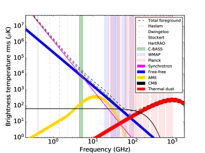
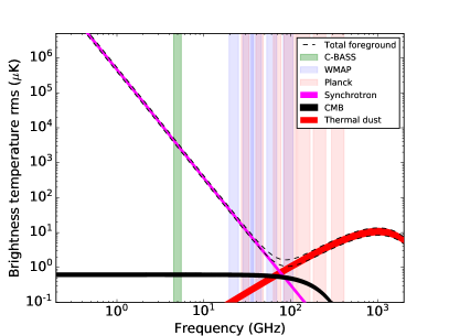
Figure 1: Frequency spectra of diffuse foregrounds in temperature (left) and polarization (right). Black solid line: CMB temperature and $E$-mode polarization; Magenta line: synchrotron; Blue line: free-free; Red line: thermal dust; Yellow line: anomalous microwave emission; black dashed line: sum of foreground components. The lines indicate the rms fluctuation level in each continuum component from the Planck Collaboration et al. (2016d) model (except for the $E$-mode polarization), evaluated at 1° FWHM resolution, for the region outside the Planck 2015 HFI Galactic plane masks that include 80 and 90 per cent of the sky (shown by the bottom and top edges of the lines respectively). Underlaid are the bands of Planck, WMAP, C-BASS, and the lower frequency radio surveys. The $E$-mode polarization amplitude has been taken from Planck Collaboration et al. (2016d), and is calculated from the best-fit power spectrum.

It remains to be seen whether GMIMS and S-PASS will be sufficiently free of scanning artefacts and far sidelobes to be useful in constraining the total intensity foreground spectrum. However, such artefacts are less important for determining rotation measures for two reasons. Firstly, in the Faraday-thin regime the position angle-wavelength relation closely follows the simple law: $\chi(\lambda)=\chi_{0}+{\rm RM}\lambda^{2}$. This allows an internal consistency check and rejection of outlier data. Secondly, Faraday rotation causes order unity changes (including sign changes) to the measured Stokes $Q$ and $U$ parameters. Consequently low-level artefacts have much less impact than on modeling the Stokes $I$ spectrum, where we are interested in spectral index variations that may change the intensity ratio between 1.4 and 5 GHz by 10 per cent or less.

Between the C-BASS and WMAP frequencies, the only large-scale survey is the QUIJOTE experiment at 11–19 GHz (Génova-Santos et al., 2015a, b), which only covers the northern sky. Unlike C-BASS, QUIJOTE does not aim to accurately recover very large-scale sky structures, and it is much less sensitive to the foreground emission, which fades rapidly with frequency. However, QUIJOTE does cover the frequencies over which the anomalous microwave emission rises rapidly to prominence, and will provide very useful constraints on this component, especially along the Galactic plane, where component separation is most complicated. The GEM 5 GHz survey Barbosa et al. (2006) is at the same frequency and resolution as C-BASS. It will cover a limited range of declinations in the southern hemisphere in polarization only (not intensity), and may provide a useful cross-check on the C-BASS South observations.

3 CMB Foregrounds

In this section we summarise the properties of the main foreground components that are known, and review how the new C-BASS data will help with the problem of cleaning foregrounds from CMB observations. We focus on ‘low’ frequencies ($\lesssim 100$ GHz) where synchrotron, free-free, AME and CMB emissions dominate. At high frequencies ($\gtrsim 100$ GHz), thermal dust dominates the sky and has been mapped in detail by new observations from Planck (Planck Collaboration et al., 2015a, c), which complement the data from low-frequency surveys such as C-BASS.

Fig. 1 shows the frequency spectra of diffuse foregrounds in intensity and polarization, based on the modelling by Planck Collaboration et al. (2016d). At very low frequencies ($<1$ GHz), synchrotron radiation invariably dominates due to its steep spectrum, while at higher frequencies ($\approx 10$–100 GHz), free-free and AME are stronger. In polarization, synchrotron dominates up to frequencies of $\approx 80$ GHz or higher (Dunkley et al., 2009; Planck Collaboration et al., 2016d; Krachmalnicoff et al., 2016). These typical spectra show that these diffuse components of radiation emit over a similar range of frequencies with spectra that are hard to discern from each other. In particular, at frequencies around the peak of the CMB spectrum (150 – 250 GHz) the spectrum of the CMB is very similar to that of synchrotron emission. Strong spectral lines (e.g., CO and HCN rotational transitions) can also have a significant impact on the broad-band intensities measured by the CMB spacecraft (e.g., Planck Collaboration et al., 2014d). The broad-band detectors used in most CMB experiments cannot distinguish between line emission and the surrounding continuum, so both components have to be modelled to give the expected signal in a given frequency channel.

While the total foreground signal is tightly constrained by the observations, the decomposition into components is currently quite uncertain, with different model assumptions capable of changing the ratio of synchrotron to AME power at 30 GHz by a factor of two (Planck Collaboration et al., 2016f). Of course this is one of the main motives for surveys such as C-BASS, which as we demonstrate in Section 7 will substantially improve the situation.

3.1 Synchrotron Emission

Synchrotron radiation is the dominant low-frequency foreground and will be the one most constrained by C-BASS. It is produced by cosmic ray leptons (electrons and positrons) spiralling in the Galactic magnetic field (Rybicki & Lightman, 1979). The radio spectrum of a single component of synchrotron radiation is well approximated by a power-law over a wide range of frequencies, with brightness temperature $T_{B}(\nu)\propto\nu^{\beta_{S}}$, which derives from a power-law distribution of cosmic-ray energies, $N(E)\propto E^{2\beta_{S}+3}$. Since the local cosmic ray lepton energy spectrum is extremely smooth in log-frequency space (Aguilar et al., 2014), and the frequency range of interest 1.5–150 GHz maps to only one decade of particle energy, the basic synchrotron spectrum is also extremely smooth. However, both intrinsic and line-of-sight effects can cause the spectrum to deviate from a simple power law, complicating the process of fitting and removing synchrotron emission from CMB maps (e.g. Chluba et al., 2017). Both the observed radio spectrum (e.g., de Oliveira-Costa et al., 2008; Kogut, 2012), and direct measurement of the local cosmic-ray lepton spectrum (e.g., Adriani et al., 2011; Aguilar et al., 2014) show significant spectral curvature at a few GHz, corresponding to particle energies of $\sim 5$ GeV, giving a net change in the spectral index $\beta_{S}$ from about $-$2.6 at a few hundred MHz to about $-$3.1 above 10 GHz (e.g., Strong et al., 2011). Although spectral curvature in synchrotron radiation is often attributed to radiative energy losses, such losses in the interstellar medium cannot explain a spectral break at this energy, and hence it must be attributed to a feature in the ill-understood injection mechanism that supplies the Galactic cosmic ray population. In addition to these causes of intrinsic spectral curvature, it is expected that on long lines of sight through the Galaxy, i.e., at low Galactic latitudes, the superposition of regions with different spectral indices will tend to flatten the observed synchrotron spectrum at higher frequencies. Observations at very low frequencies will thus tend to underestimate the synchrotron contribution at frequencies near to the foreground minimum unless this curvature is taken into account. We can thus expect that multiple measurements of the synchrotron component across the microwave band will be required in order to determine the spectral shape to the accuracy required for future $B$-mode observations.

Our knowledge of the spectrum of intensity of Galactic synchrotron radiation comes primarily from sky surveys at 0.4 GHz (Haslam et al., 1982), 1.4 GHz (Reich & Reich, 1986), 2.3 GHz (Jonas et al., 1998), and 23 GHz (WMAP; Bennett et al., 2003; Gold et al., 2011); see Table 1. Maps of the spectral index across the sky based on radio total intensity (Lawson et al., 1987; Reich & Reich, 1988; Davies et al., 1996; Platania et al., 1998, 2003; Bennett et al., 2003; Dickinson et al., 2009; Gold et al., 2011) and microwave polarization from WMAP (Fuskeland et al., 2014; Vidal et al., 2015) and S-PASS (SPASS2018) show variations in the range $-4.4<\beta<-2$. The flattest spectra are found along the Galactic plane, and are probably due to free-free emission (and absorption, at the lowest frequencies). Apparent large-amplitude variations in spectral index are also found in the regions of weakest synchrotron emission at high latitudes, which are most susceptible to the artefacts discussed in Section 2. The most reliable maps tend to show the smallest-amplitude variations. Nevertheless, after correction for the free-free contribution there is good evidence for genuine spatial variations of intensity spectral index, with slightly flatter spectra along the Galactic plane (Planck Collaboration et al., 2015d) and in the ‘haze’ near the Galactic centre (Dobler & Finkbeiner, 2008; Planck Collaboration et al., 2013). Individual supernova remnants (SNR) and pulsar wind nebulae (PWN), usually taken as the major sources of Galactic cosmic rays, typically have flatter spectra than the diffuse synchrotron, from $\beta_{S}=-2$ to $-2.3$ for PWN and $-$2.4 to $-$2.8 for shell SNR (Green, 2014; Planck Collaboration et al., 2016b). Polarized spectral indices will not necessarily be the same as in intensity, due the summing over different polarization angles within the volume probed by the beam. SPASS2018 observe that the average spectral index between 2.3 GHz and the 23 – 33 GHz WMAP and Planck bands is $-3.22$ independent of angular scale, but with significant spatial variations that are not simply due Galactic latitude. These variations will complicate efforts to extrapolate synchrotron contamination to the CMB foreground minimum frequencies.

Because synchrotron emission does not dominate the total intensity foreground in the space microwave band ($\sim 20$–$300$ GHz), attempts at component separation have effectively extrapolated it from the most reliable of the low-frequency templates, i.e. the 408 MHz survey. This long frequency baseline, and the poorly quantified variable slope and curvature of the spectrum, make this one of the main sources of uncertainty in component separation. The synchrotron-dominated data from C-BASS, at much higher frequency, will substantially reduce this uncertainty (e.g., Errard et al., 2016). Further reliable surveys between 5 and 30 GHz would improve the situation even more, as this would tightly constrain measurements of both the spectral index and spectral curvature as a function of sky position.

3.1.1 Loops, spurs and the haze

C-BASS will provide a new look at diffuse Galactic synchrotron and free-free emission. Given its modest resolution and high brightness sensitivity, this will be especially valuable for faint, large-scale structures at intermediate and high Galactic latitude. Of course, the synchrotron total intensity on these scales is mapped with high signal-to-noise ratio at 408 MHz by Haslam et al. (1982); however, it is clear from WMAP and Planck that more structure is apparent in polarization; in particular, the synchrotron loops and spurs are seen with much higher contrast in the polarization images (Planck Collaboration et al., 2016f). These features are relatively local, but there may also be a contribution from the Galactic halo. Even the weighted average WMAP and Planck data are not sensitive enough to detect the polarized emission in the faintest regions, but C-BASS will detect it everywhere, and hence address the issue of whether the inter-loop high-latitude emission is a distinct (e.g., halo) component, in which case it may have a discernibly different spectrum, or whether it is produced by numerous overlapping structures similar to the visible loops, but fainter.

Of particular interest is the WMAP/Planck haze (Planck Collaboration et al., 2013), identified as excess emission at $\approx 1$ cm partly coincident with the Fermi $\gamma$-ray bubbles (Dobler et al., 2010; Ackermann et al., 2014) which appear to delineate a 10-kpc scale bipolar outflow from the Galactic centre. The haze is (presumably) synchrotron emission with a flatter spectral index ($\beta\approx-2.5$) than the rest of the sky ($\beta\approx-3.0$). However, because of its low signal-to-noise ratio in the satellite data, and the uncertainty in foreground separation, it is not clear if the haze is really a distinct component rather than simply a trend to flatter spectral index in the inner Galactic halo, let alone whether it is related to the bubbles (see e.g., Planck Collaboration et al., 2016f). Including C-BASS in the component separation analysis should pin down the spectrum of the haze and reveal whether it has a well-defined boundary and to what extent it matches the $\gamma$-ray structures.

3.1.2 Polarized synchrotron and Faraday rotation

Optically thin synchrotron radiation has an intrinsic polarization of 70–75 per cent, oriented perpendicular to the projected magnetic field in the source region (Rybicki & Lightman, 1979). Although reduced in practice by superposition of different field directions along the line of sight, observed polarization fractions can exceed 30 per cent (e.g., Vidal et al., 2015). Because these regions may have different spectral indices, polarized and unpolarized spectra may differ, and need to be fitted separately. In principle it should be easier to fit the polarized spectrum, since synchrotron radiation is the dominant polarization foreground below the foreground minimum; but at present this is limited by the low signal-to-noise ratio of the WMAP and Planck polarization maps, and also by large-scale systematic differences between the two surveys (Planck Collaboration et al., 2016d) which indicate residual systematic errors in at least one of them. The C-BASS data will provide the first measurements of the polarized synchrotron emission that are both high signal-to-noise ratio, and not affected by depolarization, across most of the sky.

The Galactic magnetic field reveals itself through both Faraday rotation and through the intrinsic polarization of the Galactic synchrotron emission, which is orthogonal to the projected field direction in the plane of the sky. Only a band of a few degrees along the plane in the inner quadrants will suffer large depolarization; C-BASS will give a reliable map of projected magnetic field direction at moderate and high latitudes. These lines of sight probe the local interstellar medium in the plane and the Galactic halo above the spiral arms, and so can provide constraints on the measured tangling of the field on relatively small scales: 1° corresponds to about 3 pc for typical structures in the Population I disc, and $\sim 20$ pc for a 1-kpc scale-height halo. If the halo field is relaxed, the degree of polarization should reach a substantial fraction of the $m_{\rm max}\approx 75$ per cent expected from a uniform $B$-field; if the structure is tangled, the structure function of the polarized pattern will give the angular scale(s) of tangling, while random-walk depolarization will allow us to estimate the number of reversals on the line of sight $m\sim m_{\rm max}/\sqrt{N}$; these two approaches give independent estimates of the tangling scale as a fraction of the scale height. It will be illuminating to compare the field revealed by synchrotron polarization with the projected field traced by dust polarization in emission (Planck Collaboration et al., 2015a) and absorption (e.g., Heiles, 2000; Panopoulou et al., 2015), which give us different weighting functions on the line of sight, and, for starlight polarization, an upper limit to the distance.

At low latitudes the projected magnetic field is an average along the line-of-sight, but it still gives information about the field direction and coherence; in fact, modelling of the magnetic field pattern in the disk hinges on accurate assessment of the synchrotron fractional polarization at low latitudes, and is currently limited by our inability to distinguish synchrotron from AME in the Galactic disk (Planck Collaboration et al., 2016g).

C-BASS data will be combined with polarimetry from the GMIMS HB and S-PASS surveys to yield improved maps of the Faraday rotation of the diffuse Galactic synchrotron polarization, hence probing the Galactic magnetic field. Adding C-BASS doubles the range in $\lambda^{2}$ compared to GMIMS alone, yielding a corresponding increase in RM precision, while the precision of the intrinsic position angle will be improved by a factor of eight. Discrepancies between RM values derived in-band from GMIMS and in combination with C-BASS will reveal breakdown of the simple $\lambda^{2}$ law of Faraday rotation, as expected when there is measurable variation of Faraday depth across the beam and/or along the line of sight. Such Faraday dispersion will also be associated with depolarization, and so is expected to be seen only around the borders of regions which are strongly depolarized at the lower frequency, specifically at $|b|\la 30\degr$ in the inner quadrants for GMIMS and over a substantially smaller region for S-PASS (Wolleben et al., 2006; Carretti et al., 2013). This requires differential rotation of $\Delta RM\ga\pi/2\lambda^{2}$, i.e. $\ga 36$ and $92\mbox{$\rm\,rad\,m^{-2}$}$ at 1.4 and 2.3 GHz respectively. Where GMIMS is depolarised (almost exclusively in the southern hemisphere), we can derive RM from the combination of S-PASS and C-BASS, which increases $\Delta\lambda^{2}$ by a factor of 5.5 compared to using the intra-band $\Delta\lambda^{2}$ from S-PASS alone.

Similar depolarization at 5 GHz requires $\Delta RM\ga 440\mbox{$\rm\,rad\,m^{-2}$}$, and hence such depolarization should be restricted to very low latitudes in the inner Galactic plane ($|\ell|<50$). This entire region will be observed by C-BASS South, and its 128-channel backend (8 MHz channels) will allow us to measure RMs up to $10^{5}\mbox{$\rm\,rad\,m^{-2}$}$, an order of magnitude larger than even that at the Galactic centre ($6500\mbox{$\rm\,rad\,m^{-2}$}$, see Vidal et al., 2015). (In this region the synchrotron intensity is high enough that it will be detectable in each channel, except where strongly depolarized.)

The RM map gives a clear look at the line-of-sight structure of the field in the Faraday layer. For example, we would like to know whether it varies smoothly or characterized by abrupt current sheet transitions (Uyaniker & Landecker, 2002). When tangential to the line of sight, current sheets show up as discontinuities in RM, accompanied by “depolarization canals”. It will be particularly interesting to compare the Faraday rotation of the diffuse synchrotron emission with that of extragalactic sources and discrete Galactic supernova remnants and pulsars (e.g., Van Eck et al., 2011), which will allow us to constrain models for both the magnetic field geometry and the distribution of emitting regions along the line of sight (Jaffe et al., 2011).

3.2 Free-Free Emission

Free-free emission due to coulombic interactions of electrons with ions is produced in individual Hii regions and the diffuse warm ionized medium ($T\approx 10,000$ K). The free-free spectrum from a plasma in local thermodynamic equilibrium (LTE) is accurately known (Rybicki & Lightman, 1979; Draine, 2011); in the optically thin regime it has a near-universal form with spectral index $\beta=-2.1$ at GHz frequencies, slightly steepening ($\Delta\beta<0.05$) at frequencies of tens of GHz and higher. The steepening slightly increases as plasma temperature falls, but for the relevant temperature range the impact is barely detectable. In contrast, the transition to the optically thick regime cannot be accurately modelled at the degree-scale resolution of interest here because it depends on the brightness distribution within the beam; fortunately this only becomes a significant issue below $\sim 1$ GHz, with the brightest Hii regions on the Galactic plane showing absorption effects at 408 MHz and lower.

The well-defined spectrum makes free-free emission one of the most stable solutions in component separation analyses, at least for the distinct nebulae dominated by free-free emission up to 100 GHz and even higher (Planck Collaboration et al., 2014a). In these large Hii complexes, C-BASS data will be dominated by free-free emission, which will allow verification of the spectral index and provide constraints on free-free polarization. On the other hand the diffuse high-latitude free-free emission is weaker than other foreground components at all frequencies, making it difficult to separate based on spectral information alone. Although attempts have been made to use H$\alpha$ templates to constrain models of the high-latitude component (Dickinson et al., 2003; Finkbeiner, 2003; Draine, 2011), for various reasons this has not proved very accurate (Planck Collaboration et al., 2016f). Radio Recombination Line (RRL) surveys (e.g., Alves et al., 2015) may also provide an independent and direct tracer of free-free emission.

Free-free emission is inherently unpolarized, but low levels of polarization (a few percent) can be induced by Thomson scattering around the peripheries of Hii regions (Rybicki & Lightman, 1979), and locally could be stronger than the synchrotron emission near the foreground minimum ($\nu\approx 70$ GHz) because of the flatter free-free spectrum; as yet, this has not been detected.

As we will see in Section 7, C-BASS will dramatically improve our ability to recover the free-free emission from the Galactic warm ionized medium (WIM), including the faint WIM emission at high Galactic latitudes that is also traced by H$\alpha$. Standard models of the WIM seem to over-predict the radio free-free emission given the observed H$\alpha$ (e.g., Dickinson et al., 2003; Planck Collaboration et al., 2016f), and a more accurate free-free map allowing detailed point-for-point comparison with reasonable signal-to-noise ratio should help identify the source of the discrepancy, be it unexpectedly low $T_{e}$, scattering of H$\alpha$ by high-latitude dust, or departures from LTE. Because free-free emission comes primarily from HII regions, which are strongly clustered with the increased star formation in the Galactic plane, free-free emission dominates the narrow Galactic plane in the space microwave, and is about equal to synchrotron at 5 GHz, as early C-BASS results have shown (Irfan et al., 2015). Here C-BASS will help recover the spectrum of the subdominant synchrotron emission, which comes from distant regions of the Galactic disk.

3.3 Anomalous Microwave Emission (AME)

Anomalous microwave emission is a component of Galactic emission that is strongly correlated with thermal dust emission but has a frequency spectrum that peaks in the tens of GHz (1996ApJ...460....1K; Leitch et al., 1997); see e.g. de Oliveira-Costa et al. (2004); Davies et al. (2006); Gold et al. (2011); Ghosh et al. (2012); Planck Collaboration et al. (2014b) and Dickinson et al. (2018) for a review.

AME is clearly seen at 10 – 60 GHz with a rising spectrum at low frequencies and a steeply falling spectrum at higher frequencies, radically different from the tail of the thermal dust emission, and is very closely correlated with dust emission at IR/sub-mm wavelengths (Planck Collaboration et al., 2016f). The best example comes from the Perseus molecular cloud where the spectrum has been accurately determined (Watson et al., 2005; Planck Collaboration et al., 2011b; Génova-Santos et al., 2015b). A major problem for component separation is that the spectrum is spatially variable, with individual clouds peaking in the range at least 20 – 50 GHz (Planck Collaboration et al., 2014b, 2016f). At low latitude we expect superposition of clouds with a range of peak frequencies, so that AME can resemble free-free or synchrotron spectra rather closely: along with the variable synchrotron spectrum this is the second major cause of the large uncertainty in current component separation.

Measurements of the polarization of AME are challenging due to the weak signal and difficulties in component separation. Nevertheless, a number of measurements indicate that AME is at most weakly polarized, with upper limits of a few per cent in the space microwave band (Mason et al., 2009; Macellari et al., 2011; Dickinson et al., 2011; López-Caraballo et al., 2011; Rubiño-Martín et al., 2012; Hoang et al., 2013; Planck Collaboration et al., 2016f) and less than 0.5 per cent at lower frequencies (2017MNRAS.464.4107G).

The source of AME remains uncertain. The leading candidate is electric dipole radiation from small spinning dust grains (Draine & Lazarian, 1998a, b), but another mechanism still in play is ‘magnetic dust’, i.e., magnetic dipole emission due to thermal vibrations of ferromagnetic grains, or inclusions in grains (Draine & Lazarian, 1999). Earlier suggestions of hot ($\sim 10^{6}$ K) free-free emission (Leitch et al., 1997) and flat-spectrum synchrotron (Bennett et al., 2003), now seem unlikely due to the peaked spectrum and close correlation with FIR templates. Spinning dust possibly explains the low level of polarization and the narrow range of frequencies at which it is detected. However, Tibbs et al. (2013) and Hensley et al. (2016) cite some properties of AME that do not match expectations for spinning dust, casting serious doubt on this interpretation.

By design, the C-BASS frequency is too low for significant AME to be detected over most of the sky, which is a major reason why C-BASS substantially improves the separation of the non-AME components, as the lower space-microwave frequencies can contain both AME and synchrotron emission. If the peaked spectrum seen in examples such as the Perseus molecular cloud is typical, AME should be negligible at 5 GHz and C-BASS will provide an AME-free template for synchrotron and free-free emission, which in turn will allow clear identification of actual AME emission at space microwave frequencies. With an additional low-frequency measurement that is not contaminated by AME, it is possible to break the degeneracy between synchrotron spectral index and AME amplitude (see Section 7). Nevertheless, there may be a few lines of sight where AME is detectable, allowing C-BASS to constrain models of the low-frequency tail of its spectrum; a good example is G353.05+16.90 ($\rho$ Oph West) on $1^{\circ}$ scales, where there may still be appreciable AME at 5 GHz (Planck Collaboration et al., 2011b). If any of the dust-correlated features so evident in the WMAP and Planck-LFI maps are visible in C-BASS, this could imply a radically different emission mechanism from spinning dust.

3.4 Thermal Dust

Interstellar dust grains, with sizes ranging from a few to several hundred nanometers, absorb optical and UV starlight and re-emit via thermal vibrations in the crystal lattice, which excite electric dipole radiation (Draine, 2011). This is the dominant foreground above 70 GHz. Dust emission can be fitted with a modified blackbody, i.e., a Planck spectrum, $B(\nu,T_{\rm d})$ multiplied by an emissivity $\propto\nu^{\beta_{\rm d}}$. The latest Planck fits to the spectrum below 1 THz (Planck Collaboration et al., 2016d) give a narrow range around $\beta_{\rm d}\approx 1.53$, with an rms of 0.03 that may be dominated by fitting errors; $T_{\rm d}$ ranges from 15–27 K, with a mean $\approx 21$ K and a standard deviation of 2.2 K. However this model over-predicts the data above 1 THz, where the best-fit values are $\beta_{\rm d}\approx 1.50$ and $\langle T_{\rm d}\rangle\approx 19.6$ K (Planck Collaboration et al., 2015c).

The apparent uniformity of the dust spectrum disguises considerable spatial variation in dust properties. Planck Collaboration et al. (2014c) showed that $T_{d}$ is anticorrelated with emissivity at high Galactic latitude, the opposite of what would be expected from variations in starlight intensity, implying significant variations in the UV/optical absorption to FIR emission ratio. There are at least two, and likely more, chemically-distinct grain populations (Draine, 2011). There are certainly real spatial variations in $\beta_{D}$; for instance, the Small Magellanic Cloud has $\beta_{D}\approx 1.2$ (Planck Collaboration et al., 2011a). Laboratory-synthezised grain analogues show a range of $\beta_{D}$ and also spectral curvature (Coupeaud et al., 2011), and the observed mm-wave spectrum presumably represents whatever reasonably abundant grain population has the slowest fall-off towards long wavelengths.

Polarization of dust emission is due to anisotropic optical properties of the grains and a preferred orientation with respect to the magnetic field. Polarized optical extinction is associated with silicates (Draine, 2011), which are also believed to dominate the mm-wave dust emission (e.g., Planck Collaboration et al., 2016a; Fanciullo et al., 2015), and, as expected, the polarization angles seen in emission and absorption are strongly correlated (Planck Collaboration et al., 2015b). The intrinsic polarization fraction of thermal dust emission may be around 26 per cent (Planck Collaboration et al., 2016h); as for synchrotron radiation this is reduced by geometric depolarization, but observed polarization can reach 20 per cent, with typical values of $\approx 5$ per cent (Planck Collaboration et al., 2015a). Also as for synchrotron radiation, these effects can lead to different spectra in polarization and total intensity, and in fact the polarized spectrum is slightly steeper (Planck Collaboration et al., 2015c).

The intrinsic complexity of the dust spectrum poses a challenge for observing strategies that concentrate on frequencies above 100 GHz. Although synchrotron emission is below the dust emission in this frequency range, without effective constraints on the synchrotron spectrum, degeneracies between different dust models and residual synchrotron will compromise the accuracy of foreground separation at the levels of precision needed for accurate $B$-mode measurements. Although C-BASS measures frequencies far from the peak of the dust spectrum, removing these degeneracies in component fitting can lead to improvements in the measurements of the dust parameters through the improved fitting of the other components (see Section 7).

Table 2: Key specifications of the C-BASS survey.

	North	South
Location	OVRO	Klerefontein
	California	South Africa
Latitude	37° $14^{\prime}$N,	30° $58^{\prime}$S,
Longitude	118°$17^{\prime}$W	21°$59^{\prime}$E
Telescope	6.1 m Gregorian	7.6 m Cassegrain
Sky Coverage	$\delta>-15\aas@@fstack{\circ}6$	$\delta<28\aas@@fstack{\circ}6$
Frequency range	4.5 – 5.5 GHz
Effective centre frequency	4.783 GHz	5  GHz
Effective bandwidth	0.499 GHz	1.0 GHz
Frequency channels	1	128
Angular resolution	$45$ arcmin FWHM
Stokes coverage	$I,Q,U(V)$
Sensitivity	$\lesssim 0.1$ mK r.m.s. (per beam)

4 Survey requirements and constraints

The resolution requirement of the C-BASS survey is partly set by that of the complementary surveys at other frequencies and partly by the science goals, but it is also limited by practical constraints. WMAP and Planck have resolutions at their lowest frequencies of $\approx 48$ arcmin and $\approx 33$ arcmin respectively, while the 408 MHz Haslam et al. map has a nominal resolution of $51$ arcmin. In order to remove foregrounds at the angular scale of the peak of the $B$-mode power spectrum at $\ell\approx 90$, a resolution of around 1° is required. The resolution is also ultimately set by the size of antenna available, and the need to under-illuminate it to minimise sidelobes. With a 6.1-m antenna available, it was possible to design for a beam FWHM of $45$ arcmin. This is slightly better than the resolution of the Haslam map and sufficient to clean CMB maps well in to the region of the $B$-mode power spectrum peak.

Ideally C-BASS would detect polarized emission across the entire sky. To estimate the level of polarized emission at high Galactic latitudes, and hence the sensitivity required, we extrapolated from the WMAP K-band polarization map. Assuming a mean temperature spectral index of $\beta=-3$, we estimate that the polarized intensity at 5 GHz will be greater than 0.5 mK over 90 per cent of the sky. We therefore set a sensitivity goal of 0.1 mK per beam in polarization. This corresponds to about 14 mJy in flux density sensitivity. At this sensitivity level the C-BASS intensity map will be confusion limited. We estimate the confusion limit from the source counts in the GB6 survey (Gregory et al., 1996), which can be modelled as $N(S){\rm d}S=76\,(S/{\rm Jy})^{-2.44}\,{\rm Jy^{-1}\,sr^{-1}}$. With a beamsize of $45$ arcmin the expected confusion limit from extragalactic sources is about 85 mJy, corresponding to 0.6 mK, for an upper flux density limit of 100 mJy (roughly the individual source detection level in C-BASS maps). In practice the confusion limit will be somewhat lower than this, since the source counts are known to flatten at lower flux density levels than the lower limit of GB6. The polarization maps will not be confused, as the typical polarization fraction of extragalactic sources is only a few per cent. It will also be possible to correct the C-BASS intensity maps for source confusion using data from higher resolution surveys such as GB6 and PMN (Griffith & Wright, 1993). The overall specifications of the C-BASS survey are summarized in Table 2.

4.1 Survey Design

In order to map the entire sky with sensitivity to all angular scales up to the dipole, the only feasible instrument architecture is a total power scanning telescope. An interferometer is not feasible because of the difficulty in obtaining information on scales larger than the inverse of the shortest baseline. To cover the entire sky from the ground required two instruments, one in each hemisphere, situated at latitudes that give significant overlap in the sky coverage to ensure continuity on large scales between the two halves of the survey and good cross-calibration. We also require sensitivity to both intensity and polarization.

In order to construct a sky map with good accuracy on large angular scales we require a scan strategy with long continuous sweeps of the sky and good cross-linking of scans (i.e., each pixel is crossed by several scans in different directions). For intensity measurements we also choose to use a fixed reference temperature rather than a differential measurement that switches out signal at the separation angle between the beams. We scan at constant elevation to minimise the variation in atmospheric emission and ground spillover during a scan, . The survey strategy is therefore to make constant-elevation scans over the entire azimuth range, at the maximum slew rate that the telescope can manage. Maximising the slew rate pushes the signal frequency band in the time-ordered data as far as possible away from any residual $1/f$ noise in the receiver noise power spectrum. The fastest convenient azimuth slew rate for both C-BASS telescopes is 4 deg/sec. We actually use several different slew rates close to 4 deg/sec so that any systematics in the data that are at fixed frequency (for example, related to the receiver cold head cycle frequency or the mains frequency) do not always map to the same angular scale on the sky. The telescope is slewed at full speed from 0° to 360° azimuth, and then decelerates, halts, and turns around. This gives a small region of overlap in azimuth coverage and ensures the whole sky is covered at full slew speed. We also have full sky coverage in both clockwise- and anti-clockwise-going scans.

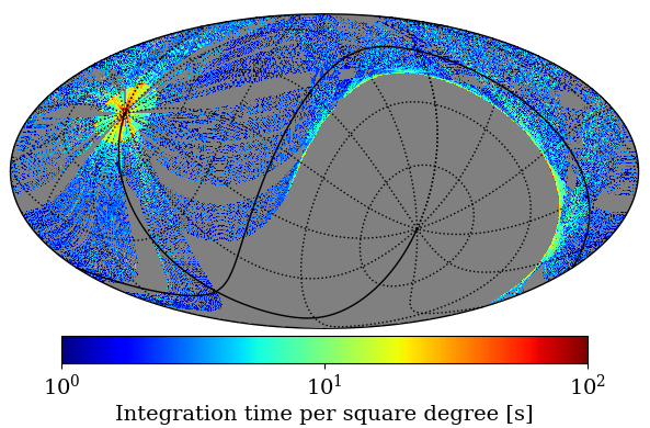
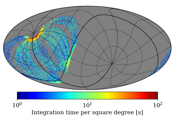
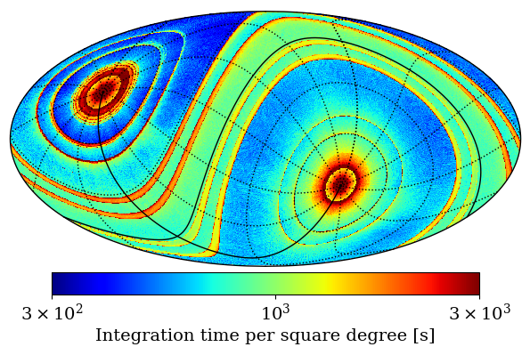
Figure 2: Top: Sky coverage from roughly one day of observations with C-BASS north, using scans at a single elevation going through the north celestial pole (elevation $37\degr$). The map is in Galactic coordinates, with an equatorial co-ordinate grid overlaid. Middle: Sky coverage from scans at an elevation ten degrees above the celestial pole (elevation $47\degr$), showing how these scans fill in the sky coverage at mid declinations. Bottom: Complete sky coverage expected from northern and southern surveys combined, using data from all elevations.

Scanning at constant elevation equal to the latitude of the observing site $\phi$ results in the scans always passing through the celestial poles, and the entire sky is eventually covered down to declination $\delta=-90\degr+2\phi$ (in the northern hemisphere). Scanning through the pole has the additional benefit that the same point on the sky is observed every scan, giving an immediate check on the drifts in offsets due to the atmosphere of the receiver. However, the resulting sky coverage is very non-uniform, with deep coverage at the pole and at the lower declination limit, but much sparser coverage at intermediate declinations. In order to get sufficient integration time over the whole sky we also observe at higher elevations, with about 60 per cent of the survey time spent at the elevation of the pole and decreasing amounts of time spent at 10, 30 and 40 degrees above the elevation of the pole. This results in a much more uniform sky coverage (see Figure 2).

For scans at a given elevation, any residual ground spillover signal will be a fixed function of telescope azimuth. The azimuth at which any given declination on the sky is observed is also fixed (in fact each declination is observed at two azimuths, symmetrically placed about the meridian), which means there is a degeneracy between the ground spillover and the sky for sky modes that are circularly symmetric about the pole (these are the $m=0$ modes in the spherical harmonic decomposition of the sky in equatorial coordinates). This degeneracy can be partly broken by observing at different elevations, which have somewhat different ground-spillover profiles, and by using the overlap region between the northern and southern surveys, which will have quite different ground-spill profiles. With the northern telescope at latitude $\phi=+37\degr$ and the southern telescope at latitude $\phi=-31\degr$ the overlap region between the two surveys is from declination $\delta=+28\degr$ to $\delta=-16\degr$. This overlap region also allows for extensive calibration cross-checks between the two surveys.

The telescopes observe continuously day and night, with calibration observations (including sky dips) inserted roughly every two hours. No attempt is made to synchronize scans, as the sky is covered many times in the course of the survey observations. Contamination from the Sun or Moon is assessed after the observations, and the final survey data will be tested empirically for residual contamination. This gives us the maximum freedom to include good data, but the survey timing is planned such that even using strictly night-time only data will give sufficient integration time.

5 Instrument design

5.1 Overview

The two C-BASS systems, north and south, have been designed to produce a single unified survey, and have many features in common. However there are some significant differences in implementation between the two systems, some forced by practical constraints, and others due to improvements in technology and lessons learned between the northern system, which was designed first, and the southern system. The two telescopes (see Figure 3) are similar in size but differ in numerous details. The northern telescope was donated to the project by the Jet Propulsion Laboratory, having been designed as a prototype for an array element for the Deep Space Network (Imbriale & Abraham, 2004). It has a 6.1-m single-piece reflector with focal ratio $f/D=0.36$. The southern telescope was donated by Telkom SA to SKA South Africa and was originally designed for the ground segment of a low-earth orbit telecommunications satellite constellation. It has a segmented 7.6-m primary with twelve radial panels, and also has a focal ratio of $f/D=0.36$. However, since the same area of the primary is illuminated as on the northern antenna, i.e. a 6.1 m diameter, the effective focal ratio of the southern antenna is 0.46. This difference results in our having to use different optical configurations for the two telescopes – the northern antenna uses Gregorian optics, while the southern antenna uses Cassegrain optics. Nevertheless, the two antennas have very well-matched beams (Holler et al., 2013). The northern receiver is an all-analogue system (King et al., 2014), while the southern receiver (Copley et al., in prep.) implements the same architecture with a digital back-end that also provides spectral resolution within the band.

5.2 Optics

A total-power scanning telescope is vulnerable to scan-synchronous systematics, i.e., spurious signals appearing in the time-ordered data at the same frequency as astronomical signals. The most obvious cause of such contamination is pick-up of the ground and other non-astronomical sources of radiation in the sidelobes of the antenna. To mitigate this, we have designed the optics to minimize the far-out sidelobes as much as possible. This is achieved by designing an optical system with minimal blockage and scattering, and very low edge illumination. Full details of the optical design are given by Holler et al. (2013). Given that we only had on-axis telescopes available, we were constrained to use a blocked aperture, rather than an off-axis unblocked design. The secondary mirror blockage results in unavoidable near-in sidelobes, which can however be quite accurately modeled and measured, and hence corrected for in the map analysis. Far-out sidelobes were minimized by having the secondary mirror supported on a transparent dielectric material rather than using metal struts. This also has the effect of maintaining the circular symmetry of the optics and thus minimizing cross-polarization. We also used a feed horn with very low sidelobes, which minimizes direct coupling between the feed and the ground when the telescope is pointed to low elevations.

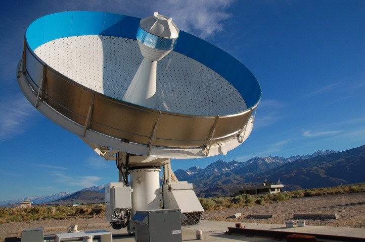
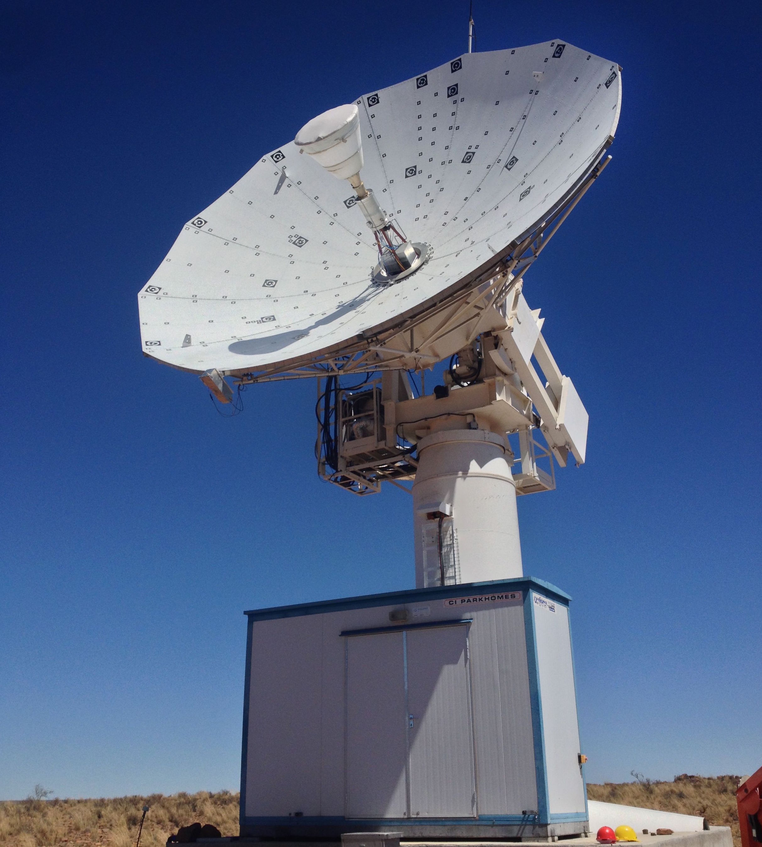
Figure 3: Top: The C-BASS North telescope, located at the Owens Valley Radio Observatory in California, U.S.A. Bottom: The C-BASS South telescope, located in the Karoo desert, South Africa. The weather shield around the receiver is removed in this image, showing the lower part of the feed horn and cryostat.

The feed is a profiled corrugated horn that generates HE12 modes in a cosine-squared section, which are phased up with the dominant HE11 mode in a cylindrical final section, resulting in a beam pattern with very low sidelobes and cross-polarization. In both telescopes the feed is well forward of the dish surface, and the entire receiver assembly is mounted above the dish surface. The feed to subreflector distance is less than 1 m in each case, which allows the subreflector to be mounted off the receiver assembly using a structure made of Zotefoam Plastazote, a nitrogen-blown polyethylene foam. This foam has very low dielectric constant and RF losses, and allows the subreflector to be supported without the use of struts that would cause scattering and break the circular symmetry of the antenna.

To minimize far-out sidelobes and hence reduce ground pick-up, the northern telescope has absorptive baffles around the primary and secondary mirrors. The primary baffle intercepts radiation that would otherwise spill over the side of the dish to the ground, while the secondary baffle reduces direct radiation from the feed to the sky/ground. Although these baffles increase the temperature loading on the receiver and contribute to the system temperature, they significantly reduce the scan-synchronous ground pick-up. The southern telescope has a larger (7.6-m) primary and so, when illuminated to produce the same beam size as the 6.1-m northern telescope, has extremely low edge illumination and negligible spillover lobes. The Cassegrain design of the southern telescope means that a baffle around the secondary mirror is not possible.

Even better rejection of ground pick-up could be achieved by surrounding the telescopes with a reflecting ground screen that shields the horizon. This would mean that the environment seen by the telescope is all at the temperature of the sky, which is around two orders of magnitude colder than the ground. Unfortunately the large size of ground screen required to shield the telescopes and still allow access to a reasonable range of elevations on the sky was too expensive to build.

5.3 Radiometer and polarimeter

The C-BASS receivers (King et al., 2014, Copley et al., in prep.) measure both intensity and linear polarization. The intensity measurement uses a continuous-comparison radiometer, which compares the power received by the antenna to a stabilized load signal, using the same gain chain for both signals so that gain instabilities in the electronics can be effectively removed. The same basic design has been used in previous instruments such as the Planck Low Frequency Instrument (Bersanelli et al., 2010). In this design, a four-port hybrid is used to form two linear combinations of the feed and reference signals, which are then both amplified, before being separated with a second hybrid and the powers of each signal detected and differenced. Gain fluctuations in the amplifiers affect both feed and reference signals equally, and are therefore cancelled out. This cancellation is continuous and does not rely on a switching frequency, and is more efficient than a Dicke switch (Dicke, 1946), in which half the integration time is spent looking at the reference load. To protect against gain fluctuations in the detectors, which come after the sky and load signals have been separated, phase switches are introduced in to the two gain arms. A single ideal 180-degree phase switch in one arm will cause the feed and reference signals to swap between the two detectors, allowing cancellation of detector gain differences. Non-ideal performance of the phase switch (e.g., different gains in the two phase states) are cancelled out by placing phase switches in both arms, and cycling between all four states of the two switches.

Polarization is measured by taking the complex correlation of the right and left circular polarizations, which yields $Q$ and $U$ directly as the real and imaginary parts of the correlation:

$$\langle|E_{R}|^{2}+|E_{L}|^{2}\rangle = I$$ (1)

$$\langle E_{R}E_{L}^{*}\rangle = (Q+iU)/2$$ (2)

$$\langle E_{L}E_{R}^{*}\rangle = (Q-iU)/2$$ (3)

$$\langle|E_{R}|^{2}-|E_{L}|^{2}\rangle = V$$ (4)

where complex amplitudes $E_{R,L}=(E_{x}\pm iE_{y})/\sqrt{2}$ multiply the propagator $\exp[i(kz-\omega t)]$ (Hamaker & Bregman, 1996). This means that $Q$ and $U$ are measured simultaneously and continuously, without needing any polarization modulation or physical rotation. This is more accurate than taking either the difference in power of the individual linear polarizations, or correlating linear polarizations, both of which require subtracting quantities involving the total intensity in order to obtain the much smaller linear polarization signal. Intensity fluctuations in the right and left channels from the unpolarized atmospheric background, and from the low-noise amplifiers, are uncorrelated and appear in the $Q$ and $U$ measurements only as noise terms. Stokes $V$ can in principle be obtained from the difference of the intensities in right and left circular polarization (Eqn. 4). However, astronomical circular polarization is expected to be extremely small, and accurate measurement of $V$ would require very precise calibration of the individual intensity measurements. In practice the $V$ signal is used as a check of the relative calibration of the intensity channels.

5.4 Cryogenic receivers and analogue electronics

The receivers for the two C-BASS telescopes are similar but differ in some significant details (King et al., 2014, Copley et al., in prep.). The cryostat bodies are very similar, and both use two-stage Gifford-McMahon coolers. The northern receiver uses a Sumitomo Heavy Industries (SHI) SRDK-408D2 cold head, which cools the second stage to 4 K. The southern receiver uses an Oxford Cryosystems Coolstar 6/30 cold head, which cools to 10 K. The southern cold head does not reach such a cold base temperature but uses significantly less compressor power (3 kW vs 9 kW for the SHI system).

Both receivers use the same design of corrugated feedhorn. The main body of the feedhorn is at ambient temperature and is bolted directly to the cryostat body. The upper section of the feedhorn also provides the support for the secondary mirror assembly. The smooth-walled throat section of the horn is machined directly into the first-stage heat shield of the cryostat, and the orthomode transducer (OMT) is mounted onto the second-stage cold plate. The 4-probe OMT (Grimes et al., 2007) is connected via coaxial cables to a planar circuit that combines the linearly polarized signals and produces circularly polarized outputs. Coaxial $-30$ dB directional couplers are used to couple in the noise source signal used for calibration. The circularly polarized signals are combined with reference signals in two 180° hybrids. The reference signals are generated from temperature-stabilized matched loads controlled by an external PID controller, which provide a load temperature stable to better than 1 mK (see Figure 4).

Both receivers use LNF-LNC4$\_$8A low noise amplifiers from Low Noise Factory, which provide 40 dB of gain between 4 – 8 GHz with a typical amplifier noise temperature of 2 – 3 K. In the southern system the signals then simply leave the cryostat via stainless steel cables. In the northern system there are notch filters that remove ground-based RFI near the centre of the band, reducing the effective bandwidth in polarization from 1 GHz to 499 MHz, and shifting the effective centre frequency to 4.783 GHz.

Figure 4: Simplified block diagram of the C-BASS front end, which is common to C-BASS north and south. Key: OMT = orthomode transducer, L2C = linear to circular converter, $\Sigma,\Delta$ = sum, differencing, BPF = bandpass filter, RCP = right circular polarization, LCP = left circular polarization. L1 and L2 are matched loads.

5.5 Backends and readout

The two C-BASS receiver systems implement the same signal processing operations to generate the intensity and polarization measurements, but in very different ways (see Figure 5). The northern system is described in detail in King et al. (2014). The radiometer and polarimeter functions are implemented by analogue electronics operating on the whole RF band as a single channel. The radiometer uses 180° hybrids identical to those used in the cryostat to separate out the sky signal from the reference signals, which are then detected with Schottky diodes. Phase switches in the RF signal path cause the sky and reference signals to be alternated between the physical channels, averaging out any gain differences or drifts in the amplifier and detector chain. The data are sampled at 2 MHz following post-detection filtering to 800 kHz bandwidth, and the sky and reference signals are differenced before phase switch demodulation and integration to 10 ms samples. For the polarimeter operation, the separated sky signals are correlated using a complex analogue correlator consisting of 90° hybrids and detector diodes. Again phase switching is used to ensure gain differences do not bias the correlated outputs. The detector diode outputs are filtered, sampled, synchronously detected at the phase switch frequencies, and filtered and averaged down to 10 ms samples in an FPGA.

The southern system, by contrast, is fully digital. After further gain and bandpass filtering, the four RF signals from the cryostat are downconverted using a 5.5 GHz local oscillator to an IF band of 0 – 1 GHz. The lower sideband is used to ensure that images of strong out-of-band signals from geostationary satellites in the range 3.5 – 4.5 GHz are not aliased in to the IF bands. The IF signals are then split and filtered to give 0 – 0.5 and 0.5 – 1 GHz IFs. Two identical digital backends are then used to process each of these two frequency bands. Each one consists of a Roach FPGA board and two iADC cards (Hickish et al., 2016). The iADC cards provide dual channel sampling at 1 GHz and 8-bits resolution. The lower IF band is sampled in its first Nyquist zone, while the upper IF band is directly sampled in the second Nyquist zone with no further analogue downconversion. The Roach board uses a Xilinx Virtex 5 FPGA to carry out the signal processing tasks. The incoming signals are first channelised using a polyphase filter bank (PFB) into 64 frequency channels of bandwidth $500/64=7.8125$ MHz. The PFB provides better than 40 dB of isolation between different channels. The signals are then combined on a channel-by-channel basis to produce the radiometer and polarimeter outputs. A bank of complex gain corrections allows phase and amplitude variations across the band due to the analogue part of the signal path to be calibrated out. The sum and difference of the pairs of input channels yields the RCP and LCP signals and their respective reference load signals. These are squared and averaged to provide measures of the power in the respective sky and reference channels. Unlike the northern system, the sky and reference signals are not differenced in the real-time system but stored separately, and only differenced in the off-line software. This allows us to assess the degree of low-frequency drifts in the raw data, but which are then cancelled out when the sky and reference are differenced. The LCP and RCP voltage signals are complex correlated to produce the polarization outputs $Q$ and $U$. The data are again averaged to 10 ms samples before being read out and stored on disk by the control system.

Figure 5: Block diagrams of the C-BASS radiometer/polarimeter systems. Top: C-BASS north analogue backend, Bottom: C-BASS south digital backend. Key: $\phi$ = phase switch modulation/demodulation, $\Sigma,\Delta$ = sum, differencing, ADC = analogue to digital converter, Acc = accumulator, CMUL = complex multiply, BPF = band-pass filter, LPF = low-pass filter, Ch = channeliser, $G\rm e^{i\phi}$ = complex gain correction, Sq = square detector (evaluates $VV^{*}$ on complex voltages $V$).

6 Data analysis

6.1 Calibration

Accurate calibration is the key to the useful application of C-BASS data. It is essential to be able to calibrate the absolute intensity (temperature) scale, the relationship between polarized and unpolarized intensity, the absolute polarization angle, and the cross-polarization response of the instrument.

Tau A is by far the brightest polarized source that is unresolved at C-BASS resolution, and is visible from both observing sites. It therefore provides our primary astronomical calibration source. Observations of other bright calibrators such as Cas A are also used when Tau A is not visible (for intensity only). Observing Tau A for long continuous periods, during which the polarization angle rotates due to parallactic rotation, allows us to measure and hence correct for the non-orthogonality of the nominal $Q$ and $U$ channels. Observations of Tau A also provide the primary flux-density calibration of the data. Converting this to a temperature scale requires a knowledge of the effective area of the antenna, or equivalently of its beam pattern. We use a detailed physical model of the antenna to construct a full-sky beam pattern using the GRASP physical optics package, which is verified with comparison measurements of the main beam and sidelobes over a wide range of angles (Holler et al., 2013).

Between primary calibration observations, the gain and polarization angle response of the instrument is tracked using a noise diode. A noise diode signal is split and injected into both circular polarization channels immediately after the linear-to-circular converter, using $-30$ dB coaxial couplers. The diode is temperature stabilized in order to provide a fixed-amplitude reference signal in both intensity and polarization. The noise diode is switched on for a few seconds at the beginning of each scan, which provides a gain measurement on a timescale of minutes. It provides a constant signal in both the $I$ and $Q$ channels (in instrument co-ordinates). Phase variations between LCP and RCP in the subsequent signal chains result in some of the noise diode signal appearing in the instrumental $U$ channel. The polarization data are rotated in post-processing to put the noise diode signal wholly back into instrumental $Q$. The absolute polarization angle will ultimately be fixed by measurements using the C-BASS South telescope of a ground-based polarized calibration source, whose polarization angle can be set to $\sim 0.1$ deg accuracy.

Gains of both the intensity and polarization data derived from the noise diode are interpolated to provide a continuous relative gain correction across the entire data set. The absolute flux-density scale is set from observations of Tau A, corrected for opacity variations between the elevation of observation of Tau A and the elevation of the survey scans. Since the noise diode is effectively a source of 100% polarization (perfectly correlated between RCP and LCP), it can be used to transfer the astronomical intensity calibration to the polarized intensity calibration, so that measurements of $I$, $Q$ and $U$ are on the same scale.

The opacity is monitored by sky dip observations that are done periodically throughout the survey observations. The telescope is scanned between elevations 60° and 40° at a fixed azimuth, providing a change in airmass of about 0.4, which gives a change in background temperature of about 1.5 K. This signal is fitted to a cosec(elevation) law to derive a zenith sky temperature and hence a zenith opacity. Opacity obervations are not made below elevation 40°  to avoid contamination from ground pick-up. Opacity corrections are typically of order 1 per cent or less.

Pointing calibration is determined from cross-scans of bright radio sources, to which a beam model is fitted to obtain azimuth and elevation offsets. These are then used to fit for a pointing model incorporating collimation, axis misalignment and flexure terms. Pointing residuals are in the range of a few arcmin and are not expected to be a significant issue in data analysis.

6.2 Flagging and data correction

Given the relatively high temperature sensitivity of C-BASS (NET $\sim 2$ mK s^1/2) compared to the brightness of the sky (several K in the Galactic plane), the C-BASS time-ordered data are frequently signal-dominated rather than noise-dominated. This complicates the removal of non-astronomical signals from the data. For example, it is not possible to flag for sporadic radio-frequency interference (RFI) simply using an amplitude clip, as a threshold low enough to eliminate significant RFI would also flag much true emission in the sky. Instead we use a sky model that is interpolated onto the time-ordered data stream and subtracted. Discrepant events can then be detected and flagged. Very small pointing errors during the crossing of bright and/or compact sources can still generate significant residuals, so RFI flagging is disabled for bright parts of the sky model. RFI that is coincident with bright emission has a proportionally smaller effect on the final map, and the very high level of redundancy in the C-BASS observations, with each sky pixel being observed dozens of times, means that any residual contamination is effectively washed out in the final map. The sky model used for RFI removal is initially made using a crude RFI cut, and progressively updated with more refined edits of the time-ordered data.

The other main non-astronomical component of the data is ground pick-up, which appears as a clear pattern repeating with azimuth, and varies on timescales of many days with changes in temperature and emissivity of the ground. As with RFI removal, a sky model is used to subtract the bulk of the sky signal from the time-ordered data, and regions of high sky brightness are excluded completely. The remaining data are averaged into azimuth bins, constructing a ground profile for every day. These profiles are then subtracted from the data before map-making. This procedure also removes fixed RFI, such as from fixed radio links and geostationary satellites.

6.3 Mapping

Although the receiver has been designed to suppress $1/f$ noise in both intensity and polarization as much as possible, there are long-term variations in background level, and residual atmospheric and ground-spill emission, that are still present in the time-ordered data. Typical $1/f$ knee frequencies in real data are around 0.1 – 0.2 Hz. While drifts longer than a complete azimuth scan can be filtered from the time-ordered data, shorter drifts will appear in maps as stripes along the scan directions. However, it is possible to solve for a good approximation to the true sky map in the presence of drifts, using the redundancy introduced by the repeated coverage of every pixel in the sky many times in the total time stream. Many mapping codes have been developed to solve this problem in the context of CMB observations (e.g., Ashdown et al., 2007), either by explicitly modelling the drift signal or by solving the map-making equation using the full noise statistics of the data. We use a destriping mapper, Descart (Sutton et al., 2010), which models the time-ordered data as consisting of a true sky signal $s_{p}$ that depends on the pointing in celestial coordinates, plus an offset series consisting of a set of constant values $a_{i}$, plus stationary white noise $w_{t}$, i.e.,

$$d_{t}=P_{tp}s_{p}+F_{ti}a_{i}+w_{t}.$$

$P_{tp}$ is the pointing matrix that gives the telescope pointing direction $p$ at each time sample, and $F_{ti}$ defines the timebase on which the offsets vary. For a well-sampled data set it is possible to solve for the offset vector $a$, which Descart does using a conjugate gradient method. The offsets are then subtracted from the data, leaving a clean time-ordered data set with only white noise, which can be mapped by binning into sky pixels.

7 Potential impact of C-BASS

The C-BASS data are primarily intended to improve foreground separation for CMB analysis by breaking degeneracies that currently exist in the component separation problem. Here we make some estimates of the degree of improvement in the accuracy of CMB and foreground component parameters that can be expected from C-BASS data.

We have simulated the component separation process for a variety of mock data sets representing typical levels of foreground contamination in pixels across different regions of the sky, using the properties of existing or planned sky surveys, with and without C-BASS. We assess the ability to recover a set of input parameters describing the CMB and foregrounds, using measurements at different frequencies $\nu$ with error bars $\sigma_{\nu}$ corresponding to particular surveys (see Table 3 for the actual frequencies and sensitivities used). The simulations consider only the thermal noise on a single pixel, and thus do not include effects due to sample or cosmic variance, nor the improvement in thermal signal-to-noise from observing a larger sky area. The full set of results showing the impact of C-BASS data on component separation in a variety of sky regions with different levels of foreground contamination will be presented in a forthcoming paper (Jew et al., in prep.). Here we will show representative results for one scenario in intensity and one in polarization.

In each case, we generate mock data at each frequency for which we expect to have an observation, using a model of the foregrounds and the CMB component. We then attempt to recover the parameters from which the mock data were generated, using an MCMC fitting process. Many examples of similar techniques can be found in the literature, including FGFIT (Eriksen et al., 2006), Commander (Eriksen et al., 2008a), and Miramare (Stompor et al., 2009), and a similar methodology has been used by Hensley & Bull (2018) to explore the impact of different dust models on CMB component separation. We assign priors appropriate to the particular foreground component model. For power-law components of the form $A(\nu/\nu_{0})^{\beta}$, we use the form of the Jeffreys prior $\mathcal{P}$ suggested by Eriksen et al. (2008b), namely $\mathcal{P}(A)=1$ and $\mathcal{P}(\beta)=[\Sigma_{\nu}(\sigma_{\nu}^{-1}(\nu/\nu_{0})^{\beta}\ln(\nu/\nu_{0}))^{2}]^{1/2}$. For the CMB amplitude we use a flat prior. We also use flat priors for the amplitude and peak frequency of the AME spectrum.

We do not add noise to the mock data, so that the results are not biased by individual realisations of the noise, but simply use the noise levels $\sigma_{\nu}$ in the calculation of the likelihood in the fitting process. Thus the posterior probability density functions that we show should be interpreted as the distribution from which any particular pixel realization would be drawn, for the given set of parameters. For example, for the intensity simulations in which we assume a CMB pixel value of $75\,\mu\rm{K}$, the posterior density is the probability of obtaining a particular value for that pixel alone. A real observation would contain many pixels with different individual CMB values, and the CMB power would be inferred from the ensemble of pixels.

Table 3: The surveys and sensitivities used for the simulations. Sensitivities for the intensity simulations are for a 1° pixel while those for polarization are for a 3° pixel. The FutureSat sensitivities are taken from an early version of the LiteBIRD mission description (Matsumura et al., 2014) and are intended to be indicative of a near-future satellite mission. The effective sensitivity on the Haslam map is taken to be 10 per cent of the median map temperature, i.e. it is dominated by the overall 10 per cent calibration uncertainty rather than the thermal noise.

Survey	Frequency / GHz	$\sigma^{I}\,/\mu{\rm K_{RJ}}$	$\sigma^{P}\,/\mu{\rm K_{RJ}}$
Haslam et al	0.408	$2.5\times 10^{6}$
C-BASS	5.0	73.0	24.0
WMAP K	22.8	5.8
WMAP Ka	33.0	4.2
WMAP Q	40.7	3.5
WMAP V	60.7	3.8
WMAP W	93.5	3.9
Planck 30	28.4	2.5	1.1
Planck 44	44.1	2.6	1.3
Planck 70	70.4	3.1	1.5
Planck 100	100	1.0	0.51
Planck 143	143	0.33	0.24
Planck 217	217	0.26	0.20
Planck 353	353	0.2	0.19
Planck 545	545	0.086
Planck 857	857	0.032
FutureSat 60	60		0.052
FutureSat 78	78		0.031
FutureSat 100	100		0.020
FutureSat 140	140		0.013
FutureSat 195	195		0.0070
FutureSat 280	280		0.0038

7.1 Intensity

To simulate the data we use a simplified version of the foreground model found in Table 4 of Planck Collaboration et al. (2016d). Our model for total intensity measurements is summarized in Table 4, and consists of the following components: a single power-law synchrotron component with amplitude $A_{s}$ and spectral index $\beta_{s}$; a free-free component with a fixed electron temperature of 7000 K and effective emission measure EM; a thermal dust component with a modified blackbody spectrum with amplitude $A_{\rm d}$, an emissivity index $\beta_{\rm d}$ and a temperature $T_{\rm d}$; and a single AME component with the spdust2 spectrum (Ali-Haïmoud et al., 2009; Silsbee et al., 2011) allowed to shift in logarithmic frequency-brightness space with an amplitude $A_{\textrm{AME}}$ and peak frequency $\nu_{\rm peak}$ (following the same prescription as in Planck Collaboration et al. 2016d).

Table 4: The models used to generate foregrounds and CMB spectra. The free parameters are those fitted for in the MCMC fitting, while the fixed parameters are fixed for each model component and are not fitted for. Each model is used to generate a temperature component in Rayleigh-Jeans brightness temperature.

Component	Free parameters	Fixed parameters	Model for $T_{\rm RJ}$
Synchrotron	$A_{\rm s},\beta_{\rm s}$	$\nu_{0}=408\,{\rm MHz\,(intensity)}$	$A_{\rm s}(\nu/\nu_{0})^{\beta_{s}}$
		$\nu_{0}=30\,{\rm GHz\,(polarization)}$
Free-free	EM	$T_{\rm e}=7000\,\rm K$, $\nu_{0}=1\,{\rm GHz}$	$T_{\rm e}(1-\exp(-\tau))$
			$\tau=0.05468T_{\rm e}^{-3/2}\,{\rm EM}\,g_{\rm ff}\,(\nu/\nu_{0})^{-2}$,
			$g_{\rm ff}=\ln(\exp[5.96-\sqrt{3}/\pi\ln((\nu/\nu_{0})(T_{\rm e}/10^{4})^{-3/2})]+e)$
AME	$A_{\rm AME},\nu_{\rm peak}$		spdust2
Dust	$A_{\rm d},\beta_{\rm d},T_{\rm d}$	$\nu_{0}=545\,{\rm GHz\,(intensity)}$	$A_{\rm d}\Big{(}\frac{\nu}{\nu_{0}}\Big{)}^{\beta_{\rm d}+1}\,\frac{\exp(h\nu_{0}/k_{\rm B}T_{\rm d})-1}{\exp(h\nu/k_{\rm B}T_{\rm d})-1}$
		$\nu_{0}=353\,{\rm GHz\,(polarization)}$
CMB	$A_{\rm CMB}$	$T_{0}=2.7255\,{\rm K}$	$A_{\rm CMB}\,x^{2}e^{x}/(e^{x}-1)^{2}$,
			$x=h\nu/k_{\rm B}T_{0}$

Table 5: Recovered parameter values for the intensity simulations, with and without the inclusion of the C-BASS data point (corresponding to the posterior density estimates in Fig. 6.

Parameter	Recovered value	Recovered value	True value	Units
	(No C-BASS)	(with C-BASS)
$A_{\textrm{s}}$ @ 100 GHz	$1.33_{-1.33}^{+1.81}$	$1.84_{-0.165}^{+0.191}$	$1.86$	$\mu$K${}_{\textrm{RJ}}$
$\beta_{\textrm{s}}$	$-3.02_{-0.16}^{+0.11}$	$-3.10_{-0.026}^{+0.025}$	$-3.10$
EM	$365_{-21}^{+11}$	$362_{-4}^{+4}$	$361$	cm-6pc
$A_{\textrm{AME}}$	$701_{-39}^{+37}$	$707_{-11}^{+13}$	$708$	$\mu$K${}_{\textrm{RJ}}$
$\nu_{\textrm{peak}}$	$25.0_{-3.2}^{+3.1}$	$25.0_{-1.6}^{+1.4}$	$25.0$	GHz
$A_{\textrm{d}}$	$2080.9_{-0.11}^{+0.10}$	$2080.9_{-0.09}^{+0.09}$	$2080.86$	$\mu$K${}_{\textrm{RJ}}$
$\beta_{\textrm{d}}$	$1.545_{-0.00087}^{+0.00095}$	$1.545_{-0.00074}^{+0.00097}$	$1.545$
$T_{\textrm{d}}$	$17.480_{-0.012}^{+0.011}$	$17.481_{-0.012}^{+0.009}$	$17.480$	K
$A_{\textrm{CMB}}$	$75.4_{-2.3}^{+2.0}$	$75.0_{-1.2}^{+1.3}$	$75.0$	$\mu$K${}_{\textrm{CMB}}$

Table 6: Recovered parameter values for the polarization simulations, with and without the inclusion of the C-BASS data point, corresponding to the posterior density estimates in Fig. 8.

Parameter	Recovered value	Recovered value	True value	Units
	(No C-BASS)	(with C-BASS)
$A_{\textrm{s}}$ @ 100 GHz	$0.086_{-0.048}^{+0.149}$	$0.072_{-0.018}^{+0.021}$	$0.074$	$\mu$K${}_{\textrm{RJ}}$
$\beta_{\textrm{s}}$	$-2.37_{-0.27}^{+1.37}$	$-3.09_{-0.10}^{+0.08}$	$-3.10$
$A_{\textrm{d}}$	$0.313_{-0.023}^{+0.034}$	$0.329_{-0.019}^{+0.022}$	$0.335$	$\mu$K${}_{\textrm{RJ}}$
$\beta_{\textrm{d}}$	$0.97_{-0.96}^{+0.37}$	$1.56_{-0.50}^{+0.51}$	$1.63$
$T_{\textrm{d}}$	$65.8_{-36.6}^{+4.2}$	$65.3_{-34.9}^{+4.7}$	$24.9$	K
$A_{\textrm{CMB}}$	$-0.02_{-0.38}^{+0.09}$	$0.02_{-0.09}^{+0.06}$	$0.00$	$\mu$K${}_{\textrm{CMB}}$

We use the component separation results from Planck Collaboration et al. (2016d) to suggest values of the foreground parameters. For this example, we used a region close to the Galactic plane to illustrate a fairly severe instance of foreground contamination. We then produce mock brightness values using the foreground models plus a CMB signal. We simulate the intensity measurements in 1° pixels, since all components (including the CMB) are detected at high signal-to-noise ratio in a typical pixel. The CMB value was set to 75 $\mu$K, corresponding to the rms fluctuations on a 1° scale. Simulated observations at the central frequencies of the Haslam, Planck, WMAP and C-BASS surveys were included. For each frequency measurement we assigned thermal noise based on the achieved or expected sensitivity of the appropriate survey. These are summarized in Table 3.

Figure 6 shows the posterior density estimates (PDE) of the total intensity foreground parameters for a single 1° pixel in a region with significant AME and free-free emission. Figure 7 shows the corresponding estimates of the actual component spectra, along with the true input spectra, and Table 5 shows the numerical values for the recovered parameters. These are given as the peak posterior value and the parameter range that contains 68 per cent of the posterior volume, as the PDEs are often quite skewed and cannot be represented with a symmetrical error bar. Without the C-BASS data, the synchrotron parameters, $A_{\rm s}$ and $\beta_{s}$, are very poorly constrained. Including the C-BASS data improves the measurement of the synchrotron radiation amplitude by an order of magnitude, and reduces the error range on the spectral index from 0.27 dex to 0.05 dex. It also markedly improves the estimates of the free-free emission measure and the AME parameters, reducing the error bars on these parameters by factors of 2 – 4. There is even a small improvement on the constraints on the dust amplitude. These improvements in foreground parameter estimates result in a reduction of the errors on the measurement of the CMB amplitude in this pixel of 40 per cent.

7.2 Polarization

For the polarization simulations we did not include a free-free or AME component. Free-free emission is essentially unpolarized, while AME polarization is expected to be small, and has not yet been detected. We also set the CMB signal to zero. This represents a situation in which the $E$-mode signal has been perfectly separated out, and we are searching for a $B$-mode signal of very small amplitude. Data points at the centre frequencies of C-BASS and Planck are included, along with a set of sensitivities indicative of a near-future CMB satellite mission (‘FutureSat’), based on the early mission description of LiteBIRD (Matsumura et al., 2014).

The PDE of the polarization foreground parameters ($B$-mode) for a 3° pixel in a low-foreground region of sky are shown in Figure 8. Figure 9 shows the corresponding estimates of the component spectra, along with the true input spectra, and Table 6 summarizes the results. Including C-BASS data results in much tighter constraints on the synchrotron amplitude and spectral index, with a previously almost unconstrained spectral index now measured with an accuracy of 0.1 dex. There is also significant improvement in the dust spectral index, resulting in a reduction in the 1-$\sigma$ range on the CMB amplitude by a factor of three. Additional low-frequency points between the C-BASS and Planck frequencies would provide additional constraints on the synchrotron spectrum and lower bias on the $B$-mode amplitude measurement.

While the addition of the C-BASS data point dramatically improves the recovery of the synchrotron components and the CMB amplitude in the case of a straight synchrotron spectrum, additional complication in the synchrotron spectra will require additional observational constraints. A C-BASS-like instrument covering frequencies between 5 GHz and the lower end of the space microwave band would provide constraints on realistic synchrotron spectra, including the effects of intrinsic curvature and line-of-sight integration of different spectra. A detailed study of such an instrument, NextBASS, and its potential impact on component separation using the techniques presented here, is in preparation.

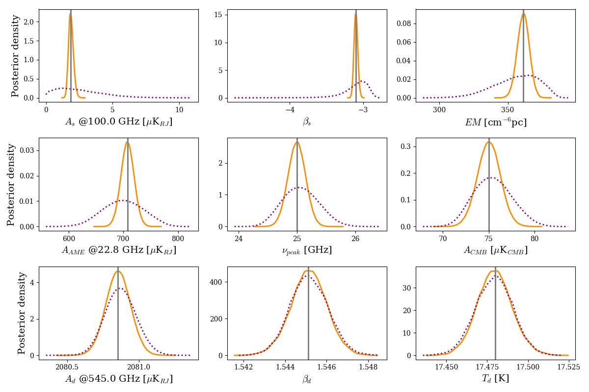
Figure 6: PDEs of the total intensity component parameters for a typical 1° pixel in a sky region with significant foreground contamination. The dashed lines are the PDEs when only including Haslam, WMAP and Planck data points in the fit. The solid lines are the PDEs when the C-BASS data point is included. The vertical lines are at the true parameter values used to simulate the data.

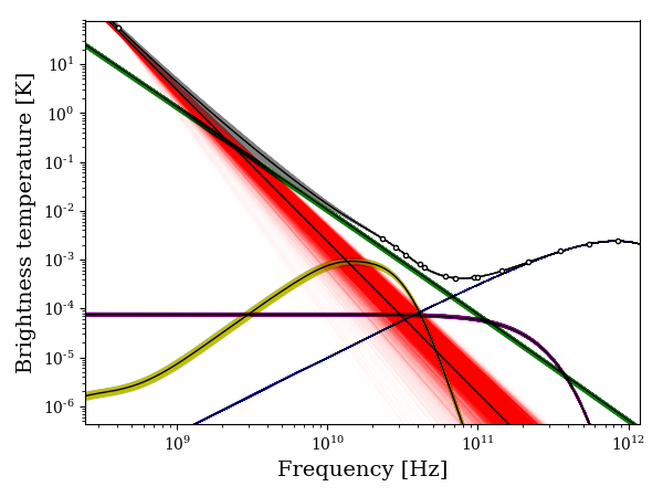
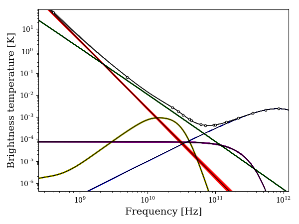
Figure 7: Total intensity frequency spectra for a 1° pixel in a sky region with significant foreground contamination. The solid black lines are spectra of the true simulated foreground components. The coloured lines are the frequency spectra of the sky components of 5000 randomly drawn samples from the converged MCMC chains. Left is the result from only including Haslam, WMAP and Planck data points. Right is with the addition of a C-BASS data point. Synchrotron is red; thermal dust is blue; AME is yellow; free-free is green; and CMB is purple.

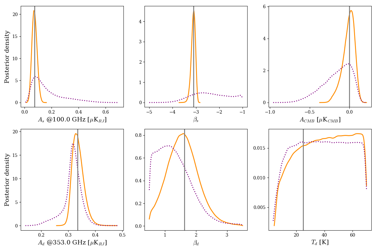
Figure 8: PDE of the $B$-mode polarization component parameters for a typical 3° pixel in a sky region with low foreground emission. The dashed lines are the PDEs when only including Planck and FutureSat data points. The solid lines are the posterior density estimates when the C-BASS data point is included. The vertical lines are at the true parameter values used to simulate the data.

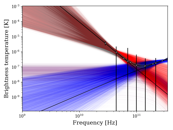
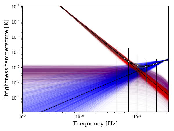
Figure 9: B-mode polarization frequency spectra for a 3° pixel in a sky region with low foreground emission. The solid black lines are spectra of the true simulated foreground components. The coloured lines are the frequency spectra of the sky components of 5000 randomly drawn samples from the converged MCMC chains. Left is the result from only including Planck and FutureSat data points. Right is with the addition of the C-BASS data point. Synchrotron is red; thermal dust is blue; and CMB is purple.

8 Conclusions

Low-frequency radio surveys are an essential component of a CMB foreground removal strategy, providing constraints on the synchrotron, free-free and AME components of Galactic emission. However, all-sky surveys to date below 20 GHz have been of limited use due to map artefacts and calibration problems. The C-Band All-Sky Survey will provide accurate and well-calibrated maps of the whole sky in Stokes $I$, $Q$ and $U$ at 5 GHz, with additional frequency resolution in the southern part of the survey. This will allow a major improvement in the accuracy of foreground separation for CMB intensity and polarization measurements. The data will also be used to study diffuse Galactic emission, such as measuring the synchrotron spectral index, constraining foreground models for studying AME at higher frequencies, and constraining models of the Galactic magnetic field.

The northern survey is now complete, with the telescope having been decommissioned in April 2015. Data reduction and analysis for the northern data are ongoing, and full results will be presented in forthcoming papers. Preliminary maps of the northern sky have been presented by moriond2018. At the time of writing, observations were still being made for the southern survey.

The C-BASS frequency at 5 GHz is the ideal balance between being sufficiently low to give good sensitivity to synchrotron radiation, with its steeply falling spectrum, and sufficiently high to avoid the worst effects of depolarization and Faraday rotation. Higher sensitivity observations at frequencies above C-BASS but below the space microwave band would of course give even better constraints on the synchrotron spectrum. C-BASS has been designed to give a clean beam with relatively high main-beam efficiency, well understood sidelobe structure, and minimal far-out and cross-polarization sidelobes. This allows accurate calibration and gives a well-understood effective temperature scale. The inclusion of C-BASS data in component separation analyses will break degeneracies in both intensity and polarization measurements, allowing more accurate estimation of foregrounds and hence of the CMB component. This additional accuracy will be crucial for future $B$-mode detections.

References

- Ackermann et al. (2014) Ackermann M., et al., 2014, ApJ, 793, 64
- Ade et al. (2014) Ade P. A. R., et al., 2014, Physical Review Letters, 112, 241101
- Adriani et al. (2011) Adriani O., et al., 2011, Physical Review Letters, 106, 201101
- Aguilar et al. (2014) Aguilar M., et al., 2014, Phys. Rev. Lett., 113, 221102
- Ali-Haïmoud et al. (2009) Ali-Haïmoud Y., Hirata C. M., Dickinson C., 2009, MNRAS, 395, 1055
- Alves et al. (2015) Alves M. I. R., Calabretta M., Davies R. D., Dickinson C., Staveley-Smith L., Davis R. J., Chen T., Barr A., 2015, MNRAS, 450, 2025
- Ashdown et al. (2007) Ashdown M. A. J., et al., 2007, A&A, 467, 761
- BICEP2/Keck and Planck Collaborations et al. (2015) BICEP2/Keck and Planck Collaborations et al., 2015, Physical Review Letters, 114, 101301
- Barbosa et al. (2006) Barbosa D., Fonseca R., Dos Santos D. M., Cupido L., Mourão A., Smoot G. F., Tello C., 2006, in Mourão A. M., Pimenta M., Potting R., Sá P. M., eds, New Worlds in Astroparticle Physics: Proceedings of the Fifth International Workshop. pp 233–237, doi:10.1142/9789812774439_0024
- Bennett et al. (2003) Bennett C. L., et al., 2003, ApJS, 148, 97
- Bennett et al. (2013) Bennett C. L., et al., 2013, ApJS, 208, 20
- Berkhuijsen (1972) Berkhuijsen E. M., 1972, A&AS, 5, 263
- Bersanelli et al. (2010) Bersanelli M., et al., 2010, A&A, 520, A4
- Calabretta et al. (2014) Calabretta M. R., Staveley-Smith L., Barnes D. G., 2014, Publ. Astron. Soc. Australia, 31, e007
- Carretti (2010) Carretti E., 2010, in Kothes R., Landecker T. L., Willis A. G., eds, Astronomical Society of the Pacific Conference Series Vol. 438, The Dynamic Interstellar Medium: A Celebration of the Canadian Galactic Plane Survey. p. 276 (arXiv:1008.4983)
- Carretti et al. (2013) Carretti E., et al., 2013, Nature, 493, 66
- Chluba et al. (2017) Chluba J., Hill J. C., Abitbol M. H., 2017, MNRAS, 472, 1195
- Coupeaud et al. (2011) Coupeaud A., et al., 2011, A&A, 535, A124
- Davies et al. (1996) Davies R. D., Watson R. A., Gutierrez C. M., 1996, MNRAS, 278, 925
- Davies et al. (2006) Davies R. D., Dickinson C., Banday A. J., Jaffe T. R., Górski K. M., Davis R. J., 2006, MNRAS, 370, 1125
- Di Bernardo et al. (2013) Di Bernardo G., Evoli C., Gaggero D., Grasso D., Maccione L., 2013, J. Cosmology Astropart. Phys., 3, 036
- Dicke (1946) Dicke R. H., 1946, Review of Scientific Instruments, 17, 268
- Dickinson et al. (2003) Dickinson C., Davies R. D., Davis R. J., 2003, MNRAS, 341, 369
- Dickinson et al. (2009) Dickinson C., et al., 2009, ApJ, 705, 1607
- Dickinson et al. (2011) Dickinson C., Peel M., Vidal M., 2011, MNRAS, 418, L35
- Dickinson et al. (2018) Dickinson C., et al., 2018, New Astron. Rev., 80, 1
- Dobler & Finkbeiner (2008) Dobler G., Finkbeiner D. P., 2008, ApJ, 680, 1222
- Dobler et al. (2010) Dobler G., Finkbeiner D. P., Cholis I., Slatyer T., Weiner N., 2010, ApJ, 717, 825
- Draine (2011) Draine B. T., 2011, Physics of the Interstellar and Intergalactic Medium. Princeton University Press
- Draine & Lazarian (1998a) Draine B. T., Lazarian A., 1998a, ApJ, 494, L19
- Draine & Lazarian (1998b) Draine B. T., Lazarian A., 1998b, ApJ, 508, 157
- Draine & Lazarian (1999) Draine B. T., Lazarian A., 1999, ApJ, 512, 740
- Du et al. (2016) Du X., Landecker T. L., Robishaw T., Gray A. D., Douglas K. A., Wolleben M., 2016, PASP, 128, 115006
- Dunkley et al. (2009) Dunkley J., et al., 2009, in Dodelson S., et al., eds, American Institute of Physics Conference Series Vol. 1141, American Institute of Physics Conference Series. pp 222–264 (arXiv:0811.3915), doi:10.1063/1.3160888
- Eriksen et al. (2006) Eriksen H. K., et al., 2006, ApJ, 641, 665
- Eriksen et al. (2008a) Eriksen H. K., Jewell J. B., Dickinson C., Banday A. J., Górski K. M., Lawrence C. R., 2008a, ApJ, 676, 10
- Eriksen et al. (2008b) Eriksen H. K., Jewell J. B., Dickinson C., Banday A. J., Górski K. M., Lawrence C. R., 2008b, ApJ, 676, 10
- Errard et al. (2016) Errard J., Feeney S. M., Peiris H. V., Jaffe A. H., 2016, J. Cosmology Astropart. Phys., 3, 052
- Fanciullo et al. (2015) Fanciullo L., Guillet V., Aniano G., Jones A. P., Ysard N., Miville-Deschênes M.-A., Boulanger F., Köhler M., 2015, A&A, 580, A136
- Finkbeiner (2003) Finkbeiner D. P., 2003, ApJS, 146, 407
- Fuskeland et al. (2014) Fuskeland U., Wehus I. K., Eriksen H. K., Næss S. K., 2014, ApJ, 790, 104
- Génova-Santos et al. (2015a) Génova-Santos R., et al., 2015a, in Cenarro A. J., Figueras F., Hernández-Monteagudo C., Trujillo Bueno J., Valdivielso L., eds, Highlights of Spanish Astrophysics VIII. pp 207–212 (arXiv:1504.03514)
- Génova-Santos et al. (2015b) Génova-Santos R., et al., 2015b, MNRAS, 452, 4169
- Ghosh et al. (2012) Ghosh T., Banday A. J., Jaffe T., Dickinson C., Davies R., Davis R., Gorski K., 2012, MNRAS, 422, 3617
- Gold et al. (2011) Gold B., et al., 2011, ApJS, 192, 15
- Green (2014) Green D. A., 2014, Bulletin of the Astronomical Society of India, 42, 47
- Gregory et al. (1996) Gregory P. C., Scott W. K., Douglas K., Condon J. J., 1996, ApJS, 103, 427
- Griffith & Wright (1993) Griffith M. R., Wright A. E., 1993, AJ, 105, 1666
- Grimes et al. (2007) Grimes P. K., King O. G., Yassin G., Jones M. E., 2007, Electronics Letters, 43, 1146
- Hamaker & Bregman (1996) Hamaker J. P., Bregman J. D., 1996, A&AS, 117, 161
- Harrington et al. (2016) Harrington K., et al., 2016, in Millimeter, Submillimeter, and Far-Infrared Detectors and Instrumentation for Astronomy VIII. p. 99141K (arXiv:1608.08234), doi:10.1117/12.2233125
- Haslam et al. (1982) Haslam C. G. T., Salter C. J., Stoffel H., Wilson W. E., 1982, A&AS, 47, 1
- Heiles (2000) Heiles C., 2000, AJ, 119, 923
- Hensley & Bull (2018) Hensley B. S., Bull P., 2018, ApJ, 853, 127
- Hensley et al. (2016) Hensley B. S., Draine B. T., Meisner A. M., 2016, ApJ, 827, 45
- Hickish et al. (2016) Hickish J., et al., 2016, Journal of Astronomical Instrumentation, 5, 1641001
- Hinshaw et al. (2013) Hinshaw G., et al., 2013, ApJS, 208, 19
- Hoang et al. (2013) Hoang T., Lazarian A., Martin P. G., 2013, ApJ, 779, 152
- Holler et al. (2013) Holler C. M., et al., 2013, IEEE Transactions on Antennas and Propagation, 61, 117
- Imbriale & Abraham (2004) Imbriale W. A., Abraham R., 2004, Interplanetary Network Progress Report, 157, 1
- Irfan et al. (2015) Irfan M. O., et al., 2015, MNRAS, 448, 3572
- Jaffe et al. (2011) Jaffe T. R., Banday A. J., Leahy J. P., Leach S., Strong A. W., 2011, MNRAS, 416, 1152
- Jonas et al. (1998) Jonas J. L., Baart E. E., Nicolson G. D., 1998, MNRAS, 297, 977
- Kamionkowski et al. (1997) Kamionkowski M., Kosowsky A., Stebbins A., 1997, Physical Review Letters, 78, 2058
- King et al. (2014) King O. G., et al., 2014, MNRAS, 438, 2426
- Kogut (2012) Kogut A., 2012, ApJ, 753, 110
- Krachmalnicoff et al. (2016) Krachmalnicoff N., Baccigalupi C., Aumont J., Bersanelli M., Mennella A., 2016, A&A, 588, A65
- Lawson et al. (1987) Lawson K. D., Mayer C. J., Osborne J. L., Parkinson M. L., 1987, MNRAS, 225, 307
- Leitch et al. (1997) Leitch E. M., Readhead A. C. S., Pearson T. J., Myers S. T., 1997, ApJ, 486, L23
- López-Caraballo et al. (2011) López-Caraballo C. H., Rubiño-Martín J. A., Rebolo R., Génova-Santos R., 2011, ApJ, 729, 25
- Macellari et al. (2011) Macellari N., Pierpaoli E., Dickinson C., Vaillancourt J. E., 2011, MNRAS, 418, 888
- Mason et al. (2009) Mason B. S., Robishaw T., Heiles C., Finkbeiner D., Dickinson C., 2009, ApJ, 697, 1187
- Matsumura et al. (2014) Matsumura T., et al., 2014, Journal of Low Temperature Physics, 176, 733
- Panopoulou et al. (2015) Panopoulou G., et al., 2015, MNRAS, 452, 715
- Planck Collaboration et al. (2011a) Planck Collaboration et al., 2011a, A&A, 536, A17
- Planck Collaboration et al. (2011b) Planck Collaboration et al., 2011b, A&A, 536, A20
- Planck Collaboration et al. (2013) Planck Collaboration et al., 2013, A&A, 554, A139
- Planck Collaboration et al. (2014a) Planck Collaboration et al., 2014a, A&A, 564, A45
- Planck Collaboration et al. (2014b) Planck Collaboration et al., 2014b, A&A, 565, A103
- Planck Collaboration et al. (2014c) Planck Collaboration et al., 2014c, A&A, 566, A55
- Planck Collaboration et al. (2014d) Planck Collaboration et al., 2014d, A&A, 571, A13
- Planck Collaboration et al. (2015a) Planck Collaboration et al., 2015a, A&A, 576, A104
- Planck Collaboration et al. (2015b) Planck Collaboration et al., 2015b, A&A, 576, A106
- Planck Collaboration et al. (2015c) Planck Collaboration et al., 2015c, A&A, 576, A107
- Planck Collaboration et al. (2015d) Planck Collaboration et al., 2015d, A&A, 580, A13
- Planck Collaboration et al. (2016a) Planck Collaboration et al., 2016a, A&A, 586, A132
- Planck Collaboration et al. (2016b) Planck Collaboration et al., 2016b, A&A, 586, A134
- Planck Collaboration et al. (2016c) Planck Collaboration et al., 2016c, A&A, 594, A1
- Planck Collaboration et al. (2016d) Planck Collaboration et al., 2016d, A&A, 594, A10
- Planck Collaboration et al. (2016e) Planck Collaboration et al., 2016e, A&A, 594, A11
- Planck Collaboration et al. (2016f) Planck Collaboration et al., 2016f, A&A, 594, A25
- Planck Collaboration et al. (2016g) Planck Collaboration et al., 2016g, A&A, 596, A103
- Planck Collaboration et al. (2016h) Planck Collaboration et al., 2016h, A&A, 596, A105
- Platania et al. (1998) Platania P., Bensadoun M., Bersanelli M., de Amici G., Kogut A., Levin S., Maino D., Smoot G. F., 1998, ApJ, 505, 473
- Platania et al. (2003) Platania P., Burigana C., Maino D., Caserini E., Bersanelli M., Cappellini B., Mennella A., 2003, A&A, 410, 847
- Reich & Reich (1986) Reich P., Reich W., 1986, A&AS, 63, 205
- Reich & Reich (1988) Reich P., Reich W., 1988, A&AS, 74, 7
- Reich et al. (2004) Reich P., Reich W., Testori J. C., 2004, in Uyaniker B., Reich W., Wielebinski R., eds, The Magnetized Interstellar Medium. pp 63–68
- Remazeilles et al. (2015b) Remazeilles M., Dickinson C., Banday A. J., Bigot-Sazy M.-A., Ghosh T., 2015b, MNRAS, 451, 4311
- Remazeilles et al. (2015a) Remazeilles M., Dickinson C., Eriksen H. K. K., Wehus I. K., 2015a, MNRAS, 451, 4311
- Rubiño-Martín et al. (2012) Rubiño-Martín J. A., López-Caraballo C. H., Génova-Santos R., Rebolo R., 2012, Advances in Astronomy, 2012
- Rybicki & Lightman (1979) Rybicki G. B., Lightman A. P., 1979, Radiative processes in astrophysics. Wiley-Interscience, New York
- Silsbee et al. (2011) Silsbee K., Ali-Haïmoud Y., Hirata C. M., 2011, MNRAS, 411, 2750
- Smoot et al. (1992) Smoot G. F., et al., 1992, ApJ, 396, L1
- Stompor et al. (2009) Stompor R., Leach S., Stivoli F., Baccigalupi C., 2009, MNRAS, 392, 216
- Strong et al. (2011) Strong A. W., Orlando E., Jaffe T. R., 2011, A&A, 534, A54
- Sun et al. (2015) Sun X. H., et al., 2015, ApJ, 811, 40
- Sutton et al. (2010) Sutton D., et al., 2010, MNRAS, 407, 1387
- Taylor et al. (2009) Taylor A. R., Stil J. M., Sunstrum C., 2009, ApJ, 702, 1230
- Tello et al. (2013) Tello C., et al., 2013, A&A, 556, A1
- Testori et al. (2008) Testori J. C., Reich P., Reich W., 2008, A&A, 484, 733
- Tibbs et al. (2013) Tibbs C. T., Scaife A. M. M., Dickinson C., Paladini R., Davies R. D., Davis R. J., Grainge K. J. B., Watson R. A., 2013, ApJ, 768, 98
- Uyaniker & Landecker (2002) Uyaniker B., Landecker T., 2002, in Cecchini S., Cortiglioni S., Sault R., Sbarra C., eds, American Institute of Physics Conference Series Vol. 609, Astrophysical Polarized Backgrounds. pp 15–19, doi:10.1063/1.1471817
- Van Eck et al. (2011) Van Eck C. L., et al., 2011, ApJ, 728, 97
- Vidal et al. (2015) Vidal M., Dickinson C., Davies R. D., Leahy J. P., 2015, MNRAS, 452, 656
- Watson et al. (2005) Watson R. A., Rebolo R., Rubiño-Martín J. A., Hildebrandt S., Gutiérrez C. M., Fernández-Cerezo S., Hoyland R. J., Battistelli E. S., 2005, ApJ, 624, L89
- Wolleben et al. (2006) Wolleben M., Landecker T. L., Reich W., Wielebinski R., 2006, A&A, 448, 411
- Wolleben et al. (2009) Wolleben M., et al., 2009, in Strassmeier K. G., Kosovichev A. G., Beckman J. E., eds, IAU Symposium Vol. 259, Cosmic Magnetic Fields: From Planets, to Stars and Galaxies. pp 89–90 (arXiv:0812.2450), doi:10.1017/S1743921309030117
- Wolleben et al. (2010a) Wolleben M., Landecker T. L., Hovey G. J., Messing R., Davison O. S., House N. L., Somaratne K. H. M. S., Tashev I., 2010a, AJ, 139, 1681
- Wolleben et al. (2010b) Wolleben M., et al., 2010b, ApJ, 724, L48
- Zaldarriaga & Seljak (1997) Zaldarriaga M., Seljak U., 1997, Phys. Rev. D, 55, 1830
- de Oliveira-Costa et al. (2004) de Oliveira-Costa A., Tegmark M., Davies R. D., Gutiérrez C. M., Lasenby A. N., Rebolo R., Watson R. A., 2004, ApJ, 606, L89
- de Oliveira-Costa et al. (2008) de Oliveira-Costa A., Tegmark M., Gaensler B. M., Jonas J., Landecker T. L., Reich P., 2008, MNRAS, 388, 247