On the distribution of spontaneous potentials intervals in nervous transmission

Abstract

One of the main challenges in Biophysics teaching consists on how to motivate students to appreciate the beauty of theoretical formulations. This is crucial when the system modeling requires numerical calculations to achieve realistic results. In this sense, due to the massive use of software, students often become a mere users of computational tools without capturing the essence of formulation and further problem solution. It is, therefore, necessary for instructors to find innovating ways, allowing students developing of their ability to deal with mathematical modelling. To address this issue one can highlight the use of Benford’s law, thanks to its simple formulation, easy computational implementation and wide possibility for applications. Indeed, this law enables students to carry out their own data analysis with use of free software packages. This law is among the several power or scaling laws found in biological systems. However, to the best of our knowledge, this law has not been contemplated in Cell Biophysics yet. Beyond its vast applications in many fields, neuromuscular junction represents a remarkable substrate for learning and teaching of complex system. Thus, in this work, we applied both classical and a generalized form of Benford’s Law, to examine if electrophysiological data recorded from neuromuscular junction conforms the anomalous number law. The results indicated that nerve-muscle communications conform the generalized Benford’s law better than the seminal formulation. From our electrophysiological measurements a biological scenario is used to interpret the theoretical analysis.

Keywords: anomalous numbers, biophysics, nervous transmission, Benford’s law

1 Introduction

The strong interdisciplinary character of Neuroscience and Biophysics opens wide possibilities for learning several quantitative aspects of biological systems. However, due to several reasons, teaching Biophysics modeling still represents a challenge [1]. Among factors one can mention the inappropriate introduction of the phenomenon prior the theoretical model development and the lack of motivating didactic sequence. In order to overcome this challenges, one can highlight a counterintuitive law, represented by a logarithmic distribution function, also known as First Digit Law or ”Law of anomalous numbers”. It was firstly discovered by polymath Simon Newcomb in $1881$, but only after $57$ years the seminal observation was revisited and popularized thanks to the physicist Frank Benford, analyzing different amount of data. Since then, the scientific community consolidated this peculiar numerical pattern as Benford’s Law (BL) [2, 3]. As it is shown in table 1 this law predicts the proportional frequency of each leading digit.

Table 1: Theoretical logarithmic law (the number zero can not be the first significant digit).

• First digit	$1$	$2$	$3$	$4$	$5$	$6$	$7$	$8$	$9$
  Frequency(%)	$30.1$	$17.6$	$12.5$	$9.7$	$7.9$	$6.7$	$5.8$	$5.1$	$4.6$

According BL, the probabilities for occurrences of leading digits is inferred by:

$$P_{i} = \log_{10}\left(\frac{i+1}{i}\right),\qquad i\in\left\{1,2,3,...,9\right\}.$$ (1)

Beyond the seminal heuristic formulation, sophisticated mathematical descriptions for explaining the significant first digit existence has been proposed. In this framework, many important properties were systematically discovered. For instance, Pinkham argued that if BL obeys some universal distribution, then this law should be scale invariant to the units chosen [4]. In these scheme, if data follows BL, they must exhibit a base invariance profile that is expressed in any other base [5]. In fact, Hill contributed with a rigorous statistical pillar, inserting the law as a branch of modern probability theory, showing that invariance uniquely implies BL [5]. To quantify how data tends to the frequencies predicted by BL, many explanations arose including the resurgence of the classical argument given by Newcomb. From Benford findings one can elaborate a crucial question: Is it BL ubiquitous in nature? Investigations have shown distinct phenomena, which apparently do not obey the law despite displaying the typically asymmetric distribution. Examples corroborating a non ubiquity argument include seismic activity, distribution of the Discrete Cosine Transform and quantized JPEG coefficients and cognition experiments [6, 7, 8]. Naturally, to expand the BL validity is necessary extending the pioneering formulation. Among alternative models proposed, one can highlight the generalization introduced by Pietronero et al. as written below:

$$P(n) = \int_{n}^{n+1}N^{-\alpha}dN$$ (2)

that is the differential equation:

$$\frac{dP(N)}{dN} = N^{-\alpha}$$ (3)

Solving (3) results in a $\alpha$-logarithm one obtain the solution:

$$P_{\alpha}(n) = \frac{1}{1-\alpha}\left[\left(n+1\right)^{(1-\alpha)}-n^{(1-\alpha)}\right]$$ (4)

$$= n^{(1-\alpha)}\ \ln_{\alpha}\left(\frac{n+1}{n}\right)$$ (5)

According to (5), defined as generalized BL (gBL), more frequent first digits than expected by BL implies in $\alpha>1$, while $\alpha<1$ means a first digit frequency below of the predicted percentage. As expected, when $\alpha=1$ the classical law is recovered. BL has been observed in different kinds of statistical data found in physical constants, number of cells in colonies of the cyanobacterium, alpha decay half-lives and fraud-detection [9, 10, 11, 12]. In Physiology, BL applications involve dynamical transitions in cardiac models and brain electrical activity [13, 14]. Nevertheless, BL and gBL remaining to be verified in another genuine complex system: the synaptic terminal. Cell interaction is accomplished by a complicated network of molecular signaling whose all details are not fully understood. In particular, information processing in the central nervous system (CNS) is mainly accomplished by a specialized structure called chemical synapses. Among many physiological functions, these zones are involved in nerve-muscle communication. Synaptic transmission is mediated by one or more substances called neurotransmitters [15]. The transmission is basically accomplished in the following steps: An action potential (AP) arrives in the nerve ending, promoting the depolarization of specialized proteins known as calcium channels voltage-dependent; Calcium ions flow through the channel diffusing inside the nervous terminal; into the nerve hey trigger the fusion of vesicle placed on the active zone (AZ) resulting in the releasing of neutransmitters, transmitting the impulse transmission to the neighbor cell. Figure 1 brings a more detailed view of neurotransmission steps [16].

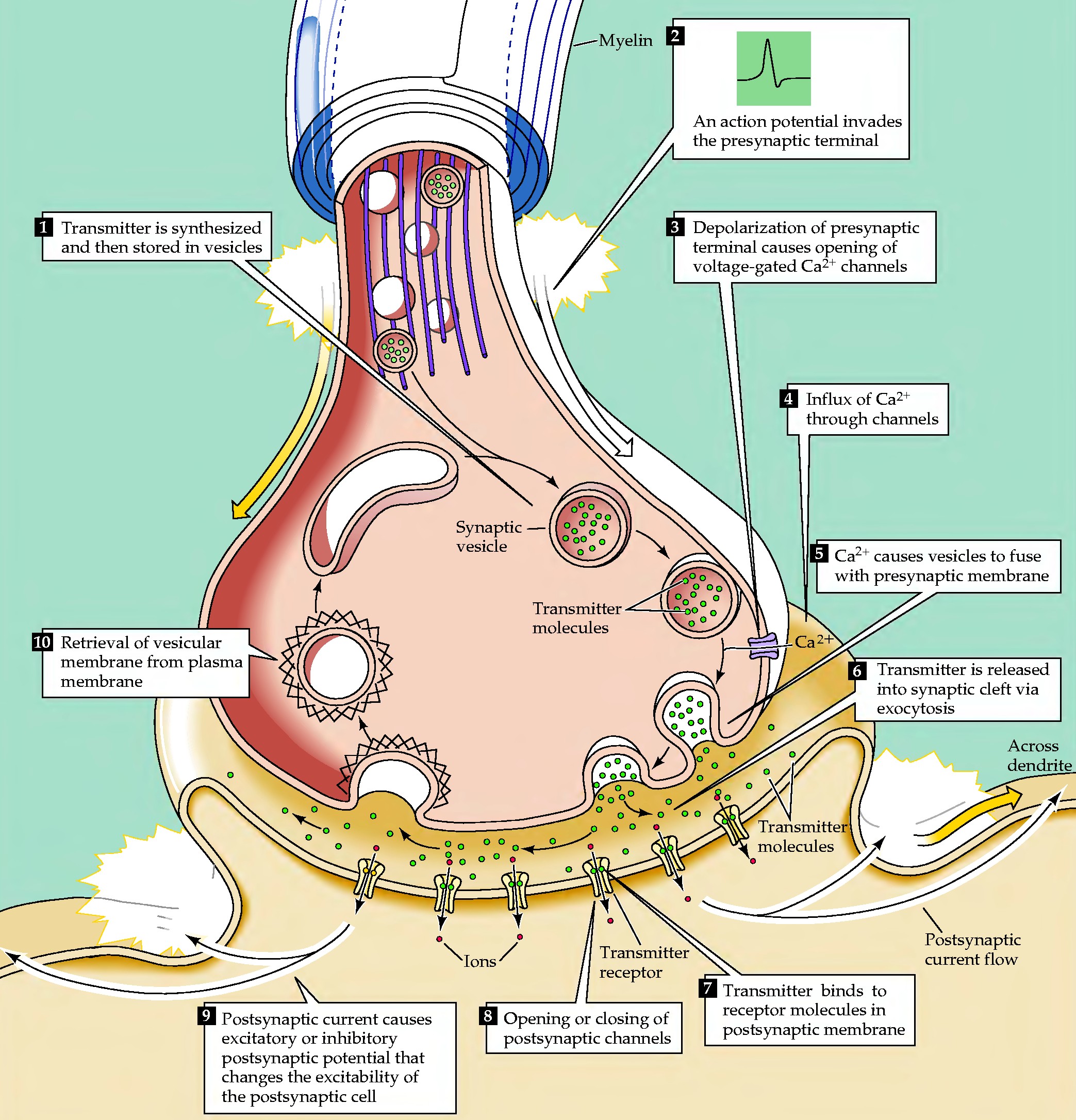
Figure 1: Sequence of events observed in a typical synaptic transmission. Figure used by permission of author [16].

The neuromuscular junction (NMJ) is responsible for communicating electrical impulses from the motor neuron to the skeletal muscle to signal contraction [17]. The terminal formed by the NMJ constitute a standard example of the well-studied chemical synapse. The facility on tissue extraction and stereotyped electrical response of nervous activity constitute the main advantages to adopt NMJ in both teaching and research. Bernard Katz led most of the pioneering work on the biophysics related to the neuromuscular transmission [18]. Using electrophysiological recordings Katz and colleagues discovered a very stereotypical spontaneous electrical activity, which plays role on the nervous terminal, called miniature end-plate potential (MEPP) [19]. These electrical signals were attributed to single vesicle fusing with the membrane terminal. Since then, NMJ established itself as the classical pillar in synaptic transmission investigation, being crucial for the understanding of mechanisms involved in neurotransmitter release. In this context, electrophysiological recordings revealed that MEPPs are no longer constant in size or temporal distribution, associating MEPPs generation as governed by Gaussian and Poisson model, respectively [20]. Katz, himself, curiously attempted to point out weaknesses in the Poissonian predictions. In fact, further introduction of a more refined experimental design, combined with powerful computational approach, exposed the nonrandom pattern embedded in several NMJ preparations [21, 22, 23]. For example, these investigations showed the fractal behavior in quantal release. Additionally, morphological studies provided a detailed scenario supporting a non-haphazard mechanism, credited to the complex physical structure of the terminal itself [24]. These structural analysis of NMJ revealed the presence of thousands of crowding vesicles sharing a very confined volume into the nerve terminal. Altogether, the arguments given above clearly configures the NMJ as a suitable preparation for several applications into education and research of Biophysics.

2 Materials and Methods

2.1 Experimental data acquisition

The experimental procedures here adopted were approved by the Animal Research Committee (CETEA - UFMG, protocol 073/03), and described more precisely in other study [25]. Briefly speaking, adult mice were euthanized by cervical dislocation, diaphragms were extracted and inserted into a physiological artificial fluid (Ringer solution) containing the following concentrations (mM): NaCl $(137)$, NaHCO₃ $(26)$, KCl $(5)$, NaH₂PO₄ $(1.2)$, glucose $(10)$, CaCl₂ $(2.4)$, MgCl₂ $(1.3)$, and pH adjusted to $7.4$ after gassing with $95\%O_{2}$ - 5% CO₂. It is valid mentioning that $[Ca^{2+}]_{o}$ physiological concentration of mammalians is about $1.8$ mM. The tissues were left bathing in the solution $30$ minutes before the electrophysiological recordings began, to minimize the mechanic trauma of their extraction. Next, tissues were gently transferred to a recording chamber continuously bathed with artificial solution at $T=24\pm 1^{\circ}{}C$. Standard intracellular recording technique was performed to monitor the frequency of spontaneous MEPP by inserting a micropipette at the chosen muscle fiber. The electrophysiological acquisition was performed using borosilicate glass microelectrodes with resistances of $8-15$ M$\Omega$ when filled with $3$ M KCl. Strathclyde Electrophysiology Software (John Dempster, University of Strathclyde), R packages [26] and Origin (OriginLab, Northampton, MA) were employed for electrophysiological acquisition and data analysis. Please see the source code, used to perform the simulations, available into Supplementary Material section. For a rigorous analysis, $33$ recordings, taken from different fibers with at least $1000$ MEPP intervals, were used. Figure 2 shows a representative segment from an electrophysiological recording.

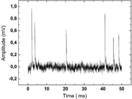
Figure 2: A representative electrophysiological recording portion showing MEPPs.

In living organisms, ions are responsible for several functions as changing solubility and melting temperature modulation of proteins. For example, potassium ions are responsible for resting membrane potential, sodium triggers the action potential generation, while calcium is crucial for the exocytosis and synaptic transmission in the ending terminal [27]. In this sense, MEPP frequency can also be manipulated by modification of the ionic concentration in Ringer solution. For this reason, the impact of $[Ca^{2+}]_{o}$ on the MEPP rate was verified assuming successive concentration (mM): $0.6$, $1.2$, $1.8$, $2.4$ and $4.8$. As a consequence, this experimental protocol enables indirectly verifying how robust is BL or gBL as function of vesicular fusion dynamics. It is also well-accepted the relationship between the membrane cellular potential and MEPP frequency. The discharge rate increases for more depolarized or positive potentials. This empirical environment may be achieved incrementing the extracellular content of potassium ($[K^{+}]_{o}$). Moreover, there are other argumentations supporting $[K^{+}]_{o}$ manipulation:(a) modulation in $[K^{+}]_{o}$ closely reproduces a physiological stimulation [28]; (b) its effects on the membrane potential in muscle preparations is well understood [29]; (c) it allows investigating BL and gBL conformity in a hyperexcitable neuronal state, by accelerating the MEPP frequency. Thus, application of BL and gBL, in conjunction with $[Ca^{2+}]_{o}$ and $[K^{+}]_{o}$ manipulation, constitute a relevant strategy to understand the scale-invariance in time series collected from electrophysiological recordings. Table 2 brings the identification for each data for different concentrations to be used in the present work.

Table 2: Ions concentrations with their respective number of MEPP and data label.

• Ion	Concentration (mM)	Data
  $Ca^{2+}_{o}$	$0.6$	$25$, $26$, $27$ and $28$
  $Ca^{2+}_{o}$	$1.2$	$19$, $20$, $29$ and $30$
  $Ca^{2+}_{o}$	$1.8$	$6$, $13$, $15$, $16$, $21$ and $22$
  $Ca^{2+}_{o}$	$2.4$	$1$, $10$, $11$, $12$, $14$, $17$ and $18$
  $Ca^{2+}_{o}$	$4.8$	$2$, $3$, $4$, $5$, $7$, $8$ and $9$
  $K^{+}_{o}$	$25.0$	$23$, $24$, $31$, $32$ and $33$

3 Results

In this work, we address if the interval between MEPPs may conform BL or gBL. In more specific terms it will be assessed the following issues:

a) Are the BL or gBL observed at physiological concentrations?

b) Is the conformity independent of the ionic concentration?

c) Is the conformity degree modulated by $[Ca^{2+}]_{o}$ and $[K^{+}]_{o}$ modifications?

d) What are the biophysical implications?

To pursue these questions, choosing reliable statistical methods is an important requirement in order to achieve reliable results. In this sense, many authors assume the $\chi^{2}$ test for verifying BL conformity, although this test manifests the ”excess of power” problem. Thus, to circumvent the ”excess of power” effect, one can use the mean absolute deviation (MAD) or sum of squares difference (SSD) as suggested for Nigrini and Kossovsky, respectively [12, 30]. According to MAD results between $0.000-0.006$ means ”close conformity”, while $0.006-0.012$ represents an ”acceptable conformity” and $0.012-0.015$ configures a ”marginal conformity”. Values higher than $0.015$ are considered ”non-conforming”. In mathematical form MAD is defined as:

$$MAD = \frac{\displaystyle\sum_{i=1}^{n}|AP_{i}-EP_{i}|}{n}$$ (6)

where AP is the actual proportion and EP is the expect proportion.

In the same way, for SSD between $0-2$, $2-25$, $25-100$ represents ”perfect conformity”, ”acceptable conformity” and ”marginal conformity”, respectively. Values above $100$ are considered ”non-conforming”. The SSD is calculated using the expression:

$$SSD = \displaystyle\sum_{i=1}^{n}\left(AP_{i}-EP_{i}\right)^{2}\times 10^{4}$$ (7)

Once again, AP is the actual proportion and EP is the expected proportion.

In this framework, using MAD and SSD, Slepkov et. al uncovered BL conformity in answers of every end-of-chapter question in introductory physics and chemistry textbooks [31]. Using the same calculations, but including the gBL calculation, both statistical methods were here used to uncover a possible conformity in MEPP intervals. The results are summarized in tables 4 and 5. Notably, SSD exhibited conformity in all cases analyzed with gBL, while conformity was computed in thirty-one cases when BL was used. Additionally, MAD revealed non-conformity in nine and five data for BL and gBL calculations, respectively. In particular, employing gBl to study physiological $[Ca^{2+}]_{o}$ recordings, a full conformity was documented in all data, while in only one case BL did not show conformity (data $13$). Figure 3 shows the results for two electrophysiological recordings ($18$ and $22$), at physiological $[Ca^{2+}]_{o}$, where a conformity was satisfactorily obtained. Curiously, two data for high $[K^{+}]_{o}$ ($23$ and $24$) did not conform BL, regardless the statistical methods. In contrast, SSD confirmed that at high $[K^{+}]_{o}$ gBL is more robust to adjust these experimental results (figure 4). This situation was similarly extracted by Pietronero et al. in their investigation using earthquake magnitude catalog. The table 3 gives a concise tabulation of the present findings.

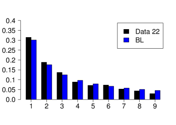
(a)                                                      (b)

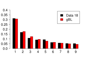
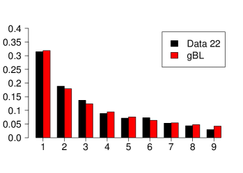
(c)                                                      (d)

Figure 3: Representative examples showing two data set for $[Ca^{2+}]_{o}$ = $1.8$ mM concentrations using BL and gBL.

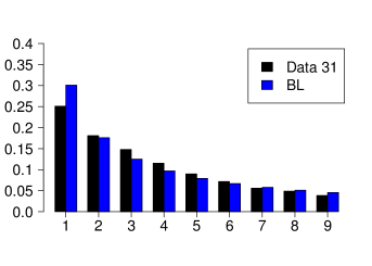
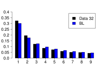
(a)                                                      (b)

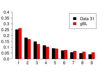
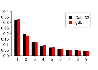
(c)                                                      (d)

Figure 4: Representative figures showing results for high $[K^{+}]_{o}$. Top: MAD and SSD calculations revealed that both data $31$ and $32$ conforms BL. Bottom: Application of gBL, both data confirmed conformity in respect of SSD and MAD analysis.

Table 3: A more synthetic presentation of the statistical analysis.

• Law	Conformity
  BL	Yes	No
  MAD	24	09
  SSD	31	02
  gBL	Yes	No
  MAD	28	05
  SSD	33	0

4 Discussion

Neurophysiology is an interdisciplinary area, propitious for the understanding of several problems in complex systems. In conjunction with available repository resources, instructors have an excellent opportunity to use novel empirical data, building a didactic sequence in modern topics of Biophysics [32]. When successful, this strategy opens an plenty room for interesting applications in teaching and research [33, 34]. In this framework, the NMJ adoption, combined with the simplicity of BL and gBL analysis, certainly provide a creative form to explore new features of the probabilistic nature of biological systems [35]. Although the regulatory releasing mechanisms require a network of molecular cascade, exocytosis may be exacerbated when $[Ca^{2+}_{o}]$ and $[K^{+}]_{o}$ increases. According to the present results, both $[Ca^{2+}_{o}]$ and $[K^{+}]_{o}$ manipulation did not show any evident modulation with the conformity degree. In other words, different concentrations did not reveal a drastic deviation from the predicted anomalous numbers behavior. Thus, the results here presented allow to establish a validity of BL and gBL at the cellular level. From these observations one can conjecture: Is the first digit law ubiquitous in the mammalian diaphragm? To address this issue it is important mentioning the necessity to verify if MEPP intervals obey the BL and gBL for other physiological parameters as, for instance, different values for pH and temperature. Indeed, many reports documented that electrical activity of NMJ is modulated by thermal changes [36]. A remarkable effect of thermal elevation is the acceleration of the vesicular fusion rate, directly reflecting in the MEPP frequency increment. Thus, this experimental maneuver constitutes a propitious inspection of how temperature may affects the degree of conformity.

Another interesting observation is the relationship between BL/gBL with nonextensive statistics [37]. Simulations carried out in astrophysical sources and studies done at the NMJ support at least an indirect relation [38]. Curiously, Pietronero calculations also offer a glimpse toward a formal mathematical connection between gBL and nonextensive theory. Relative to NMJ, Silva et al. showed that MEPP histograms are better understood when adjusted with long tails functions, e.g., q-Gaussian distribution [39]. A nonextensive behavior gives additional support for long-range correlation mechanisms playing role in the communication between nerve and muscle. Furthermore, application of Detrended Fluctuation Analysis (DFA) also uncovered long-range correlations in the MEPP intervals. Since DFA allows detects of scale-invariance in nonstationary data, the findings here reported converge with these previous studies. Thus, the results in this work support the previous theoretical studies in Neuroscience, highlighting a possibility for expanding this study including distributions governed by a lognormal dependence. This function has been applied in electrophysiological signals harvested from NMJ and brain synapses [40, 41]. In a nonextensive context, the lognormal distribution has been generalized, taking into account long-range correlations [42]. Thus, a simultaneous application of gBL and generalized lognormal function in MEPP intervals, could gives additional evidence toward a common scenario between gBL and nonextensive statistics. The present results attested that gBL emerges as a useful form to identify scale-invariance from electrophysiological time series by noting the evolution of the first digit behavior. Relationships that depending on scale-invariance can have profound implication in Physiology, being manifested in the heart, lung and brain [43, 44, 45, 46]. It is also claimed that BL observation is intimately connected to an underlying chaotic dynamical process [47]. In this context, gBL results give a supplementary support to the understanding of scale-invariant properties previously showed at NMJ by other authors [22]. In this sense, how such exocytotic machinery can organize themselves into an invariant scale scenario will be the focus of further research.

Bormashenko asked why BL is frequently observed in statistical data [48]. According to his view, like BL, many systems entropically governed are described by a logarithm dependence. This argument may explain why BL is so observed in different systems and conditions, including the results described in this work. It is worth mentioning that experiments, carried out at amphibian NMJ, also reported the intervals distribution described by a logarithm behavior [23]. Lemons conjectured another intriguing questioning, asking why there are more small things in the world than large things [49]. In keeping with this author one can paraphrase: Why short MEPP interval, given by the abundance of first digit, prevails over the others ones? Takeda et al. had already shown that most intervals concentrate at a shorter time [23]. In a physiological interpretation, such short MEPP intervals may be necessary for keeping the spontaneous synaptic activity at a more perennial or secure levels.

An important concern in Biophysics is the extrapolation of results from in vitro procedure to in vivo conditions where tissues are intact. Among disadvantages, the in vitro technique presents mechanical stress, promoted during tissue remotion, and artifacts arisen from chemical changes induced by the artificial physiological fluid [50]. These factors may mask the true electrical response of the neuronal dynamics. On the other hand, in vitro methods have many advantages, allowing a better control of several physiological variables, which are not possible using in vivo techniques. For example, isolating the neuronal cell enables elimination of efferent contribution responsible for modifying its intrinsic electrical response. Undoubtedly, as any experimental procedure, despite some limitations, in vitro techniques are consolidated as a reliable methodology, responsible for innumerable advances of Cell Biophysics. Future studies is required to verify if the BL/gBL may be observed in NMJ of non-mammalians species and pathological tissues [51, 52, 53]. It is also interesting investigating how toxins and drugs could change the first digit distribution in the MEPP intervals.

5 Concluding remarks

In summary, to the best of our knowledge, this is the first report to identify the validity of anomalous numbers law in synaptic transmission. In fact, all experimental data showed conformity with the gBL no matter the statistical method adopted. The results confirm NMJ not only as a remarkable physiological preparation in Biophysics research, but also representing an approach for teaching different topics in the scope of complex systems. In this context, the time series intervals of spontaneous potentials taken from NMJ diaphragm of mice were examined, where BL and gBL validation were robustly observed independently of $[Ca^{2+}]_{o}$ and $[K^{+}]_{o}$ manipulations. Thus, the present findings convinced us that the spontaneous quantal release conforms the anomalous number phenomenon. Last, but not least, we hope that the present work will serve to motivate the lecturer not only to include the first digit law in their courses. It is also important to propose classroom activities using the first digit law in other biophysical data obtained from repositories.

Appendix

Table 4: MAD and SSD values using BL.

• Data	1	2	3	4	5	6
  	$0.011$	$0.009$	$0.019$	$0.010$	$0.008$	$0.008$
  MAD	acceptable	acceptable	non-	acceptable	acceptable	acceptable
  	conformity	conformity	conforming	conformity	conformity	conformity
  	$25.283$	$11.748$	$69.49$	$20.831$	$7.240$	$12.285$
  SSD	marginal	acceptable	marginal	acceptable	acceptable	acceptable
  	conformity	conformity	conformity	conformity	conformity	conformity

• Data	7	8	9	10	11	12
  	$0.009$	$0.011$	$0.012$	$0.011$	$0.009$	$0.011$
  MAD	acceptable	acceptable	acceptable	acceptable	acceptable	acceptable
  	conformity	conformity	conformity	conformity	conformity	conformity
  	$10.232$	$17.011$	$26.874$	$13.062$	$12.087$	$24.118$
  SSD	acceptable	acceptable	marginal	acceptable	acceptable	acceptable
  	conformity	conformity	conformity	conformity	conformity	conformity

• Data	13	14	15	16	17	18
  	$0.020$	$0.012$	$0.010$	$0.009$	$0.008$	$0.007$
  MAD	non-	acceptable	acceptable	acceptable	acceptable	acceptable
  	conforming	conformity	conformity	conformity	conformity	conformity
  	$86.453$	$15.426$	$16.562$	$10.086$	$9.113$	$7.343$
  SSD	marginal	acceptable	acceptable	acceptable	acceptable	acceptable
  	conformity	conformity	conformity	conformity	conformity	conformity

• Data	19	20	21	22	23	24
  	$0.012$	$0.012$	$0.013$	$0.010$	$0.027$	$0.024$
  MAD	acceptable	acceptable	marginal	acceptable	non-	non-
  	conformity	conformity	conformity	conformity	conforming	conforming
  	$22.422$	$21.618$	$21.548$	$9.911$	$117.777$	$102.727$
  SSD	acceptable	acceptable	acceptable	acceptable	non-	non-
  	conformity	conformity	conformity	conformity	conforming	conforming

• Data	25	26	27	28	29	30
  	$0.014$	$0.016$	$0.021$	$0.019$	$0.019$	$0.013$
  MAD	marginal	non-	non-	non-	non-	marginal
  	conformity	conforming	conforming	conforming	conforming	conformity
  	$26.107$	$33.57$	$59.946$	$71.313$	$55.625$	$20.256$
  SSD	marginal	marginal	marginal	marginal	marginal	acceptable
  	conformity	conformity	conformity	conformity	conformity	conformity

• Data	31	32	33
  	$0.014$	$0.009$	$0.018$
  MAD	marginal	acceptable	non-
  	conformity	conformity	conforming
  	$36.178$	$11.411$	$69.913$
  SSD	marginal	acceptable	marginal
  	conformity	conformity	conformity

Table 5: Values of $\alpha$, MAD and SSD using gBL.

• Data	1	2	3	4	5	6
  $\alpha$	$0.894$	$1.091$	$1.249$	$1.157$	$1.005$	$1.097$
  	$0.011$	$0.006$	$0.014$	$0.004$	$0.008$	$0.006$
  MAD	acceptable	close	marginal	close	acceptable	close
  	conformity	conformity	conformity	conformity	conformity	conformity
  	$16.777$	$5.462$	$25.506$	$2.386$	$7.222$	$5.358$
  SSD	acceptable	acceptable	marginal	acceptable	acceptable	acceptable
  	conformity	conformity	conformity	conformity	conformity	conformity

• Data	7	8	9	10	11	12
  $\alpha$	$1.056$	$1.100$	$1.153$	$1.056$	$1.012$	$0.902$
  	$0.008$	$0.009$	$0.009$	$0.010$	$0.01$	$0.011$
  MAD	acceptable	acceptable	acceptable	acceptable	acceptable	acceptable
  	conformity	conformity	conformity	conformity	conformity	conformity
  	$7.880$	$9.861$	$9.874$	$10.672$	$11.983$	$16.802$
  SSD	acceptable	acceptable	acceptable	acceptable	acceptable	acceptable
  	conformity	conformity	conformity	conformity	conformity	conformity

• Data	13	14	15	16	17	18
  $\alpha$	$1.305$	$1.030$	$0.858$	$0.987$	$0.950$	$1.028$
  	$0.011$	$0.011$	$0.003$	$0.008$	$0.007$	$0.007$
  MAD	acceptable	acceptable	close	acceptable	acceptable	acceptable
  	conformity	conformity	conformity	conformity	conformity	conformity
  	$16.907$	$14.812$	$1.972$	$9.964$	$7.333$	$6.770$
  SSD	acceptable	acceptable	perfect	acceptable	acceptable	acceptable
  	conformity	conformity	conformity	conformity	conformity	conformity

• Data	19	20	21	22	23	24
  $\alpha$	$0.986$	$1.135$	$0.873$	$1.072$	$0.686$	$0.734$
  	$0.012$	$0.008$	$0.009$	$0.007$	$0.020$	$0.021$
  MAD	acceptable	acceptable	acceptable	acceptable	non-	non-
  	conformity	conformity	conformity	conformity	conforming	conforming
  	$22.263$	$7.807$	$9.876$	$5.968$	$45.097$	$47.660$
  SSD	acceptable	acceptable	acceptable	acceptable	marginal	marginal
  	conformity	conformity	conformity	conformity	conformity	conformity

• Data	25	26	27	28	29	30
  $\alpha$	$0.873$	$0.843$	$0.922$	$0.753$	$0.912$	$0.963$
  	$0.011$	$0.012$	$0.020$	$0.016$	$0.018$	$0.011$
  MAD	acceptable	acceptable	non-	non-	non-	acceptable
  	conformity	conformity	conforming	conforming	conforming	conformity
  	$14$	$16.372$	$55.081$	$26.039$	$50.136$	$19.217$
  SSD	acceptable	acceptable	marginal	marginal	marginal	acceptable
  	conformity	conformity	conformity	conformity	conformity	conformity

• Data	31	32	33
  $\alpha$	$0.831$	$1.105$	$0.753$
  	$0.012$	$0.004$	$0.015$
  MAD	acceptable	close	marginal
  	conformity	conformity	conformity
  	$14.640$	$3.052$	$23.739$
  SSD	acceptable	acceptable	acceptable
  	conformity	conformity	conformity

References

1. Supplementary Material

##############################################################################
################################ΨΨΨΨΨΨBenford’s LawΨΨΨΨΨΨ###############################
##############################################################################


#The code, used in this article, was created by the authors.
#R-cran repository provides two packages for analysis of Benford’s Law:
#benford.analysis and BenfordTests.
#These packages allow the user easily calculate various parameters and perform
#multiple tests on the data set.
#They can be installed using the command:
#install.packages("benford.analysis")  # Or Downloaded on the R-cran Repository:
#https://cran.r-project.org/web/packages/benford.analysis/index.html
#install.packages("BenfordTests")      # Or Downloaded on the R-cran Repository:
#https://cran.r-project.org/web/packages/BenfordTests/index.html
#R language reads many formats, we save the input data in the .csv extension.
#Read data by using the "," as decimal point.
data.bf<- read.csv(file = "NMJ-2.csv",header = TRUE,dec = ",")




###################################################################################

#########
################ΨΨΨΨUsing the Packages to Data Analyses
#########


###ΨΨEvaluate the Parameters Using the Package: benford.analysis

library(benford.analysis)ΨΨ# Activate the package: benford.analysis; that allow you:

model.ba<-benford(data.bf[,1],number.of.digits = 1) # Take the first digit from data
plot(model.ba)                                      # Plot Digits Distribution.

model.baΨΨΨ      # All information from data.
chisq(model.ba)ΨΨΨ# Calculate the Chi-Square test.
MAD(model.ba)ΨΨΨ  # Calculate the Mean Absolute Deviation (MAD) test.



###ΨΨEvaluate the Parameters Using the Package: benford.analysis

library(BenfordTests)ΨΨ# Activate the package: BenfordTests.
                                       # This package allow you:
model.bt<-data.bf[!is.na( data.bf[,1]),1]  # Remove the NA values
chisq.benftest(model.bt)               # Calculete the Chi-Square test.
ks.benftest(model.bt)                  # Kolmogorov-Smirnov test.
usq.benftest(model.bt)                 # Freedman-Watson U-square test.
mdist.benftest(model.bt)               # Chebyshev Distance test.
edist.benftest(model.bt)               # Euclidean Distance test.
meandigit.benftest(model.bt)           # Judge-Schechter Mean Deviation test.
jpsq.benftest(model.bt)                # Joenssens JP-square test.
jointdigit.benftest(model.bt)          # A Hotelling T-square type test.




###################################################################################

#########
################ΨΨΨΨParameters Calculation
#########


###ΨΨProbability of Benford’s Law.
lb<-vector(mode = "numeric"); for(i in 1:9){ lb[i]<-log10(1+1/i ) }


###ΨΨFirst Digit of Data.
first.digit<-data.bf
for(i in 1:ncol(data.bf)){ first.digit[,i]<-as.numeric( substr(data.bf[,i], 1,1) ) }


###ΨΨAbsolute and Relative Frequency of Data.
freq<-first.digit[1,] ; for(i in 1:9){ for( j in 1:ncol(first.digit)){
    freq[i,j]<-sum(first.digit[,j]==i,na.rm = T)}}ΨΨ# Absolute Frequency.                 Ψ

freq.rel<-freq[,c(1,2)] ; for( j in 1:ncol(first.digit)){ΨΨ# Relative Frequency.
    freq.rel[,j]<- freq[,j]/(sum(freq[,j],na.rm = T) ) }


###ΨΨCalculate Chi-square explicitly.
ep.qui<- colSums( ((freq.rel-lb)^(2)) /lb )* colSums(freq) ; ep.qui


###ΨΨCalculate MAD explicitly.
ep.mad<-colSums( abs( freq.rel-lb ))/9 ; ep.mad


###ΨΨCalculate SSD explicitly.
ep.ssd<-colSums( ( freq.rel-lb )^(2) )*10^(4) ; ep.ssd


###ΨΨPlot Benford’s Law Data
barplot( t(data.frame(freq.rel[,1],lb)), main = "Benford’s Law Analysis",
Ψ    Ψ    names.arg =1:9, beside = T, col= c("black","blue"),
Ψ    Ψ    legend.text = c("Data","BL"), axis.lty = 1,las=1)



###################################################################################

#########
################ΨΨΨΨGeneralized Benford’s Law for alpha
#########


###ΨΨFirst Digit of Data.
first.digit<-data.bf
for(i in 1:ncol(data.bf)){ first.digit[,i]<-as.numeric( substr(data.bf[,i], 1,1) ) }


###ΨΨAbsolute and Relative Frequency of Data.
freq<-first.digit[1,] ; for(i in 1:9){ for( j in 1:ncol(first.digit)){
              freq[i,j]<-sum(first.digit[,j]==i,na.rm = T)}}ΨΨ# Absolute Frequency.

freq.rel<-freq[,c(1,2)] ; for( j in 1:ncol(first.digit)){ΨΨ# Relative Frequency.
              freq.rel[,j]<- freq[,j]/(sum(freq[,j],na.rm = T) ) }


###ΨΨFunction - Generalized Benford’s Law.
prob.alpha<-function(alpha){ aux<- c( (2^(1-alpha) -1)/(1-alpha), (3^(1-alpha)
      -2^(1-alpha))/(1-alpha), (4^(1-alpha) -3^(1-alpha))/(1-alpha), (5^(1-alpha)
      -4^(1-alpha))/(1-alpha), (6^(1-alpha) -5^(1-alpha))/(1-alpha), (7^(1-alpha)
      -6^(1-alpha))/(1-alpha), (8^(1-alpha) -7^(1-alpha))/(1-alpha), (9^(1-alpha)
      -8^(1-alpha))/(1-alpha), (10^(1-alpha) -9^(1-alpha))/(1-alpha) )
aux<-aux/sum(aux) ; return(aux)}


###ΨΨFunction - Mean Square deviation for Alpha Variation
alpha.erro<-function(alpha){
  prob.alpha<-c ( (2^(1-alpha) -1)/(1-alpha), (3^(1-alpha) -2^(1-alpha))/(1-alpha),
        (4^(1-alpha) -3^(1-alpha))/(1-alpha), (5^(1-alpha) -4^(1-alpha))/(1-alpha),
        (6^(1-alpha) -5^(1-alpha))/(1-alpha), (7^(1-alpha) -6^(1-alpha))/(1-alpha),
        (8^(1-alpha) -7^(1-alpha))/(1-alpha), (9^(1-alpha) -8^(1-alpha))/(1-alpha),
        (10^(1-alpha) -9^(1-alpha))/(1-alpha) )
  prob.alpha<-prob.alpha/sum(prob.alpha)
  result<- sum( (prob.alpha-freq.rel[,kk])^2) ; return( result) }


###ΨΨTo Optimize the Parameter, we use the package: DEoptim.
#They can be installed using the command:
#install.packages("DEoptim")  # Or Downloaded on the R-cran Repository:
#https://cran.r-project.org/web/packages/DEoptim/index.html
library(DEoptim) # Activate the package: DEoptim. This package allow you


###ΨΨOptimize the parameter Alpha.
kk<-1  # The column number that will be
alpha.de<-DEoptim(fn=alpha.erro, lower=c(0), upper=c(10),control=list(
Ψ                       NP=200,itermax=1000,strategy=3))   #  Optimize
alpha.de$optim$bestmem[[1]]                #  Best Value for Alpha
alpha.de$optim$bestval                     #  Error
prob.alpha(alpha.de$optim$bestmem[[1]])    #  Probability of Generalized Benford’s Law


###ΨΨChi-Square - Generalized Benford’s Law
mep.qui<- colSums(  ((freq.rel[kk]-prob.alpha(alpha.de$optim$bestmem[[1]])
      )^(2)) / prob.alpha(alpha.de$optim$bestmem[[1]])  )* colSums(freq[kk])
mep.qui


###ΨΨMAD - Generalized Benford’s Law
mep.mad<-colSums( abs( freq.rel[kk]- prob.alpha(alpha.de$optim$bestmem[[1]]) ))/9
mep.mad


###ΨΨSSD - Generalized Benford’s Law
mep.ssd<-colSums( ( freq.rel[kk]- prob.alpha(alpha.de$optim$bestmem[[1]])
                     )^(2) )*10^(4)
mep.ssd



###ΨΨPlot Generalized Benford’s Law Analysis Data
barplot( t(data.frame(freq.rel[,kk], prob.alpha(alpha.de$optim$bestmem[[1]]) )),
            main = "Generalized Benford’s Law Analysis", names.arg =1:9, beside = T,
            col= c("black","red"), legend.text = c("Data","gBL"),
            axis.lty = 1,las=1)

References

- [1] Islami A and Longo G 2017 Prog. Biophys. Mol. Biol. 131 179
- [2] Newcomb S 1881 Am. J. Math. 4 39
- [3] Benford F 1938 Proc. Am. Philos. Soc. 78 551
- [4] Pinkham R S 1961 Ann. Math. Stat. 32 1223
- [5] Hill T P 1995 Statistical Science 10 354
- [6] Pietronero L, Tosatti E, Tosatti V and Vespignani 2001 Physica A 293 297
- [7] Fu D, Shi Y Q and Su W 2007 Proc. SPIE 6505 1
- [8] Gauvrit N G, Houillon J C and Delahaye J P 2017 Adv. Cogn. Psychol 13 121
- [9] Burke J and Kincanon E 1991 Am. J. Phys. 59 952
- [10] Costas E, Lopez-Rodas V, Toro F J and Flores-Moya A 2008 Aquatic Botany 89 341
- [11] Buck B, Merchant A C and Perez S M 1993 Eur. J. Phys. 14 59
- [12] Nigrini M J 2012 Benford’s Law: Applications for forensic accounting, auditing, and fraud detection (Hoboken: John Wiley & Sons)
- [13] Seenivasan P, Easwaran S, Sridhar S and Sinha S 2016 Front. Physiol. 6 390
- [14] Kreuzer M, Jordan D, Antkowiak B, Drexler B, Kochs E F and Schneider G 2014 Anesth. Analg. 118 183
- [15] Südhof T C 2013 Neuron 80 675
- [16] Purves D, Augustine G J, Fitzpatrick D, Hall W C, LaMantia A S and White L E 2012 Neuroscience 5 ed (Sunderland: Sinauer Associates)
- [17] Sanes J R and Lichtman J W 1999 Annu. Rev. Neurosci. 22 389
- [18] Katz B 2003 J. Neurocytol. 32 437
- [19] Fatt P and Katz B 1952 J. Physiol. 117 109
- [20] Bennett M R and Kearns J L 2000 Prog. Neurobiol. 60 545
- [21] Washio H M and Inouye S T 1980 J. Exp. Biol. 87 195
- [22] Lowen S B, Cash S S, Poo M and Teich M C 1997 J. Neurosci. 17 5666
- [23] Takeda T, Sakata A and Matsuoka T 1999 Prog. Neuropsychopharmacol. Biol. Psychiatry. 23 1157
- [24] Rizzoli S O and Betz W J 2005 Nat. Rev. Neurosci. 6 57
- [25] Lima R F, Prado V F, Prado M A and Kushmerick C 2010 J. Neurochem. 113 943
- [26] R Development Core Team 2008 R: A language and environment for statistical computing (Viena: R Foundation for Statistical Computing)
- [27] Rusakov D A 2006 J. Neurochem. 12 317
- [28] Grohovaz F, Fesce R and Haimann C 1989 Cell Biol. Int. 13 1085
- [29] Adrian R H 1956 J. Physiol. 133 631
- [30] Kossovsky A E 2012 Benford Law:Theory, the General Law of Relative Quantities, and Forensic Fraud Detection Applications (Singapore: World Scientific)
- [31] Slepkov A D, Ironside K B and DiBattista D 2015 PLoS ONE 10 e0117972
- [32] Halliday A C, Devonshire I M, Greenfield S and Dommett E 2010 Adv. Physiol. Educ. 34 205
- [33] Rodriguez-Falces J 2015 Adv. Physiol. Educ. 39 15
- [34] Rodriguez-Falces J 2013 Adv. Physiol. Educ. 37 327
- [35] Branco T and Staras K 2009 Nat. Rev. Neurosci. 10 373
- [36] Carlson C G, Kriebel M E and Muniak C G 1982 Neuroscience 7 2537
- [37] Shao L and Ma B Q 2010 Phys. Rev. E 82 041110
- [38] Moret M A, Senna V, Pereira M G and Zebende G F 2006 Int. J. Mod. Phys. C 17 1597
- [39] Silva A J, Lima R F and Moret M A 2011 Phys. Rev. E 84 041925
- [40] Kloot W V 1989 J. Neurosci. Methods 27 81
- [41] Buzsáki G and Mizuseki K 2014 Nat. Rev. Neurosci. 15 264
- [42] Queirós S M D 2012 Phys. A 391 3594
- [43] Bernaola-Galván P, Ivanov P C, Amaral L A and Stanley H E 2001 Phys Rev Lett. 87 168105
- [44] Fadel P J, Barman S M, Phillips S W and Gebber G L 2004 J. Appl. Physiol. 97 2056
- [45] Cai S M, Jiang Z H, Zhou T, Zhou P L, Yang H J and Wang B H 2007 Phys. Rev. E 76 061903
- [46] Gisiger T 2001 Biol. Rev. 76 161
- [47] Tolle C R, Budzien J L and LaViolette R A 2000 Chaos 10 331
- [48] Bormashenko E, Shulzinger E, Whyman G and Bormashenko Y 2016 Physica A 444 524
- [49] Lemons D S 1986 Am. J. Phys. 54 816
- [50] Azzarelli R, Oleari R, Lettieri A, Andre V and Cariboni 2017 Brain Sci. 7 48
- [51] Verschuuren J, Strijbos E and Vincent A 2016 Handb. Clin. Neurol. 133 447
- [52] Lewis R L and Gutmann L 2004 Semin. Neurol. 24 175
- [53] Shinozaki H 1980 Prog. Neurobiol. 14 121