DCPT/18/66, IPPP/18/33, MCnet-18-10 Higgs-boson plus Dijets:
Higher-Order Matching for High-Energy Predictions

Abstract

Several important processes and analyses at the LHC are sensitive to higher-order perturbative corrections beyond what can currently be calculated at fixed order. The formalism of High Energy Jets (HEJ) calculates the corrections systematically enhanced for a large ratio of the centre-of-mass energy to the transverse momentum of the observed jets. These effects are relevant in the analysis of e.g. Higgs-boson production in association with dijets within the cuts devised to enhance the contribution from Vector Boson Fusion (VBF).

HEJ obtains an all-order approximation, based on logarithmic corrections which are matched to fixed-order results in the cases where these can be readily evaluated. In this paper we present an improved framework for the matching utilised in HEJ, which for merging of tree-level results is mathematically equivalent to the one used so far. However, by starting from events generated at fixed order and supplementing these with the all-order summation, it is computationally simpler to obtain matching to calculations of high multiplicity.

We demonstrate that the impact of the higher-multiplicity matching on predictions is small for the gluon-fusion (GF) contribution of Higgs-boson production in association with dijets in the VBF-region, so perturbative stability against high-multiplicity matching has been achieved within HEJ. We match the improved HEJ prediction to the inclusive next-to-leading order (NLO) cross section and compare to pure NLO in the $h\to\gamma\gamma$ channel with standard VBF cuts.

1 Introduction

Fixed-order perturbation theory delivers a good description of inclusive rates of collider-processes involving jets; however, logarithmic corrections of various origins are important for observables in different regions of phase space. For example, the detailed description of the dependence of the cross-section on jet-sizes $R$ receives systematic logarithmic perturbative corrections of the type $\alpha_{s}^{n}\ln^{n}1/R$[1, 2]. These logarithms are controlled by DGLAP-like evolution equations, which also govern the formalism of parton showers[3, 4, 5]. While corners of phase space characterised by large ratios of transverse scales are well described by the parton-shower formalism, measurements at D0 at 1.96 TeV[6] and ATLAS at 7 TeV[7] indicate clearly that even when matched with fixed-order matrix elements, the parton showers do not describe well the regions of large invariant mass or large rapidity spans of the jet systems. This region of phase space is of particular interest in the process $pp\to Hjj$, with contributions (at Born level) of $\alpha_{w}^{2}$ through weak boson fusion and $\alpha_{s}^{4}$ through gluon-fusion (GF). It is reasonable to distinguish the two contributions to the same final state, since the quantum interference is negligible[8, 9, 10]. The impact of the radiative corrections to each process is rather different though; in particular, the $t$-channel colour octet exchange in the gluon-fusion process leads to increased jet-activity[11], which allows for a distinction of the production mechanism within the phase space populated by weak boson fusion. The two jets in weak boson fusion are often separated by a large invariant mass and rapidity span. This is the phase-space region where the perturbative corrections for the QCD processes contain logarithms of $\log(\hat{s}_{jj}/p_{t}^{2})$ from Balitsky-Fadin-Kuraev-Lipatov (BFKL)[12, 13, 14, 15]. These logarithms are contained within the formalism of High Energy Jets, where the systematic treatment is obtained by a power-expansion of the scattering matrix element in $\hat{s}/p_{t}^{2}$[16, 17]. The first sub-leading corrections were presented for the process of $Hjj$ in Ref.[18] by calculating the leading behaviour of certain sub-leading processes. This constitutes control of a well-defined set of NLL BFKL logarithms within HEJ. These logarithms drive the pattern of further emissions from the QCD process[11], which will allow for a better discrimination between the GF and VBF processes than what could be performed by investigating the dynamics of just two jets in the event.

The formalism of HEJ captures leading logarithmic terms to processes with at least two jets at large partonic centre-of-mass energy, of the form $\alpha_{s}^{k}\ln(\hat{s}/p_{\perp}^{2})^{k}\simeq\alpha_{s}^{k}\Delta y_{j_{f}j_{b}}^{k}$, where $\Delta y_{j_{f}j_{b}}$ is the rapidity-difference between the jets forward and backward in rapidity. The systematic treatment of these terms is based on a logarithmic all-order expansion point-by-point in phase space of the leading virtual corrections to all orders, combined with a power-expansion (in $\hat{s}/p_{t}^{2}$) of the square of the tree-level matrix elements, again point-by-point in the $n$-particle phase space. Upon integration, the leading power-expansion of the square of the matrix elements ensure the appropriate logarithmic accuracy of cross sections. The contributions for $n>2$ are numerically integrated over phase space, allowing for detailed jet clustering and event analyses.

Within the formalism of HEJ, the $m$-jet rates entering each prediction are matched to tree-level accuracy point-by-point in phase space, by the following procedure for mapping the $n$-parton resummation phase space point into a $m$-parton tree-level phase space point, described in more detail in Ref.[19] and Section 2:-

1. cluster the $n$-parton phase space point into jets with a chosen jet algorithm and jet $p_{t}$-threshold (e.g. anti-kt clustering, with a threshold of 30 GeV)

2. remove the partons not forming part of the hard jets from the event, and distribute the sum of their transverse momenta onto the hard jets

3. adjust the energy and longitudinal momentum of each jet such that it is on-shell, while keeping their rapidities fixed

4. adjust the momenta of the incoming partons such that energy and momentum conservation is restored

The result of this procedure is a set of momenta for which the on-shell $m$-jet tree-level matrix element can be evaluated. This in turns allows for the weight of the generated event to be reweighted to full tree-level $m$-jet accuracy, thus obtaining full tree-level accuracy up to the multiplicity for which the tree-level matrix elements can be evaluated in reasonable time. This method for matching the all-order results to fixed-order high-multiplicity matrix elements has been used for matching all results obtained with HEJ: jets, and $\gamma$, $Z$, $W$ plus at least two jets with matching up to 4 jets, and $H$ with at least two jets, with matching up to 3 jets.

The matching procedure described here can thus be viewed as merging the results of fixed-order calculations by use of the power-expanded matrix elements of HEJ coupled with the logarithmic virtual corrections, similarly to the CKKW-L–method[20, 21] of using the logarithmic accuracy of a shower-algorithm to merge fixed-order cross sections of varying multiplicity. This paper will present a complete reformulation of the procedure for merging and all-order summation. With the same input (as in use of the same matrix elements to the same order), the results are unchanged, but the new procedure for obtaining the all-order results and the merging will allow for merging results beyond tree-level, and will be computationally much more efficient.

In Section 2 we describe the original mechanism for matching leading-order samples within HEJ before a detailed discussion of the new formulation. This includes both analytical aspects and practical aspects of implementation. In Section 3 we study the results obtained in the new formalism in the context of Higgs boson plus dijets in three studies. Firstly we confirm that when matching to fixed order samples is limited to a maximum of three jets, we find consistent results with the previous formalism. Secondly, we study the impact of increasing the multiplicity in the fixed-order samples, now possible for the first time. Thirdly, we compare the matched all-order results of HEJ with those obtained at next-to-leading order accuracy. In Section 4, we conclude with a final discussion.

2 Matching

In the original formulation, the cross sections within HEJ are calculated by explicitly constructing the all-order result by first generating a $2\to n+l$ kinematic point for each number of partons $n=2,\ldots,N$, where $N$ is chosen sufficiently large (in practice around 22), and $l$ describes the non-partonic particles produced, e.g. $Z,W,H$ or their decay products. In order to simplify the notation we will only discuss the purely partonic case. Likewise, we will restrict our discussion to the leading-logarithmic contribution. Note that all our arguments apply equally to the more general scenario. We demonstrate this by showing results for the production of a Higgs boson in association with at least two jets, including recently computed sub-leading corrections [18].

The high-energy limit is dominated by Fadin-Kuraev-Lipatov (FKL) configurations, where two partons scatter in such a way that there is no radiation outside the rapidity range spanned by the scattering partons and only gluons are emitted inside this range. To ensure the high-energy limit applied is valid, it is required that the extremal (in rapidity) partons are perturbative (hard in terms of transverse momentum), and are members of the extremal jets. The transverse momenta of the remaining partons are all generated down to effectively $\mathrm{𝟎}$ GeV, technically to a very small scale of order 200 MeV (which can be varied), below which there is perfect cancellation between the subtraction terms (used in the organisation of the cancellation of the IR divergences [18]) and the real-emission terms. The matching to LO accuracy for all $m$-jet rates, $m\leq n$, is then obtained by first projecting the kinematics of the generated all-order events into Born kinematics according to the number of hard jets as described in the previous section. The event weight is multiplied with a ratio of the square of the full Born-level matrix element to the HEJ approximation of the same. The cross section (and kinematic distributions) is then obtained through the formula:-

$$\begin{split}\sigma_{2j}^{\mathrm{resum,match}}=&\sum_{f_{1},f_{2}}\ \sum_{n=2}^{\infty}\ \int_{p_{1\perp}=p_{\perp,\mathrm{min}}}^{p_{1\perp}=\infty}\frac{\mathrm{d}^{2}\mathbf{p}_{1\perp}}{(2\pi)^{3}}\ \int_{p_{n\perp}=p_{\perp,\mathrm{min}}}^{p_{n\perp}=\infty}\frac{\mathrm{d}^{2}\mathbf{p}_{n\perp}}{(2\pi)^{3}}\ \prod_{i=2}^{n-1}\int_{p_{i\perp}=\lambda}^{p_{i\perp}=\infty}\frac{\mathrm{d}^{2}\mathbf{p}_{i\perp}}{(2\pi)^{3}}\\ &\times\ \mathbf{T}_{y}\prod_{i=1}^{n}\left(\int\frac{\mathrm{d}y_{i}}{2}\right)\ \times\frac{\overline{|\mathcal{M}_{\mathrm{HEJ}}^{\text{reg}}(\{p_{i}\})|}^{2}}{\hat{s}^{2}}\times\ \sum_{m}\mathcal{O}_{mj}^{e}(\{p_{i}\})\ w_{m\mathrm{-jet}}^{\mathrm{LO}}\\ &\times\ \ x_{a}f_{a,f_{1}}(x_{a},Q_{a})\ x_{b}f_{b,f_{2}}(x_{b},Q_{b})\ (2\pi)^{4}\ \delta^{2}\!\!\left(\sum_{i=1}^{n}\mathbf{p}_{i\perp}\right)\ \mathcal{O}_{2j}(\{p_{i}\}),\end{split}$$ (1)

where $|\mathcal{M}_{\mathrm{HEJ}}^{\text{reg}}(\{p_{i}\})|^{2}$ is the square of the regularised all-order matrix element within HEJ for the $2\to n$ phase space point (see Ref.[18] for further details), and

$$w^{\mathrm{LO}}_{m\mathrm{-jet}}\equiv\frac{\overline{\left|\mathcal{M}_{\text{LO}}^{f_{1}f_{2}\to f_{1}g\cdots gf_{2}}\left(\left\{p^{B}_{\mathcal{J}_{l}}(\{p_{i}\})\right\}\right)\right|}^{2}}{\overline{\left|\mathcal{M}_{\text{LO, HEJ}}^{f_{1}f_{2}\to f_{1}g\cdots gf_{2}}\left(\left\{p^{B}_{\mathcal{J}_{l}}(\{p_{i}\})\right\}\right)\right|}^{2}}$$ (2)

is the ratio between the square of the matrix element evaluated at full tree-level accuracy and within HEJ for the state projected to tree-level $2\to m$ kinematics described by the jet momenta $\left\{p^{B}_{\mathcal{J}_{l}}(\{p_{i}\})\right\}$. $\mathcal{O}_{mj}^{e}(\{p_{i}\})$ is the exclusive $m$-jet measure applied to the generated event kinematics. $\mathbf{T}_{y}$ indicates rapidity ordering. The limits of the integral over the transverse momentum of the extremal partons combined with the two-jet measure is set to guarantee that the extremal partons carry the dominant momentum of the extremal jets. We choose a cut-off $p_{\perp,\mathrm{min}}$ corresponding to 90% of the transverse momentum of the respective extremal jet. We use here the phrase ‘kinematics of the generated all-order event’ to mean the $n$-parton kinematic point of the resummation event sampled in Eq. (1). In order to match each $m$-jet rate to tree-level accuracy, each generated event in the all-order phase-space is mapped to a $m$-jet tree-level kinematic point, and requires an evaluation of the full $m$-jet matrix element.

The scale-variation of the normalisation of the cross sections is determined by the tree-level matrix elements, and mostly unchanged by the leading logarithmic (LL) high-energy resummation implemented in HEJ. This could be reduced by extending the reweighting factor $w_{m-\mathrm{jet}}$ to next-to-leading order accuracy. However, in order to do this, one would have to integrate over all $m+1$ parton real emission phase space resulting in a specific $m$-jet Born level kinematics. This would be prohibitively time-consuming. An opposite approach is to begin with fixed order samples of exclusive jet rates and then merge these using HEJ to generate all-order results. We demonstrate how to do this in the next subsection and find significant benefits already at tree-level accuracy. In particular, each phase space point used for the tree-level matrix element maps into all the relevant resummation phase space points which leads to fewer evaluations of the tree-level matrix elements. This in turn allows for matching to higher multiplicity for a given CPU envelope.

2.1 Supplementing Fixed Order Samples with HEJ Resummation

The reformulation of the resummation and matching should reproduce the results of Eq. (1). Starting from this equation, we introduce a $\delta$-functional and an integration over the Born level kinematics of the on-shell, reshuffled jets $\{j_{B}^{i}\}$ reconstructed from the resummed kinematics. Eq. (1) is rewritten to

$$\sigma {}_{2j}^{\mathrm{resum,match}}=\sum_{f_{1},f_{2}}\ \sum_{m}\prod_{j=1}^{m}\left(\int_{p_{j\perp}^{B}=0}^{p_{j\perp}^{B}=\infty}\frac{\mathrm{d}^{2}\mathbf{p}_{j\perp}^{B}}{(2\pi)^{3}}\ \int\frac{\mathrm{d}y_{j}^{B}}{2}\right)\ (2\pi)^{4}\ \delta^{(2)}\!\!\left(\sum_{k=1}^{m}\mathbf{p}_{k\perp}^{B}\right)$$

$$\times\ x_{a}^{B}\ f_{a,f_{1}}(x_{a}^{B},Q_{a}^{B})\ x_{b}^{B}\ f_{b,f_{2}}(x_{b}^{B},Q_{b}^{B})\ \frac{\overline{\left|\mathcal{M}_{\text{LO}}^{f_{1}f_{2}\to f_{1}g\cdots gf_{2}}\big{(}\big{\{}p^{B}_{j}\big{\}}\big{)}\right|}^{2}}{(\hat{s}^{B})^{2}}$$

$$\times\frac{w_{m\mathrm{-jet}}}{\overline{\left|\mathcal{M}_{\text{LO}}^{f_{1}f_{2}\to f_{1}g\cdots gf_{2}}\big{(}\big{\{}p^{B}_{j}\big{\}}\big{)}\right|}^{2}}\ \times(2\pi)^{-4+3m}\ 2^{m}$$

$$\times\ \sum_{n=2}^{\infty}\ \int_{p_{1\perp}=p_{\perp,\mathrm{min}}}^{p_{1\perp}=\infty}\frac{\mathrm{d}^{2}\mathbf{p}_{1\perp}}{(2\pi)^{3}}\ \int_{p_{n\perp}=p_{\perp,\mathrm{min}}}^{p_{n\perp}=\infty}\frac{\mathrm{d}^{2}\mathbf{p}_{n\perp}}{(2\pi)^{3}}\ \prod_{i=2}^{n-1}\int_{p_{i\perp}=\lambda}^{p_{i\perp}=\infty}\frac{\mathrm{d}^{2}\mathbf{p}_{i\perp}}{(2\pi)^{3}}\ (2\pi)^{4}\ \delta^{(2)}\!\!\left(\sum_{k=1}^{n}\mathbf{p}_{k\perp}\right)$$

$$\times\ \mathbf{T}_{y}\prod_{i=1}^{n}\left(\int\frac{\mathrm{d}y_{i}}{2}\right)\ \mathcal{O}_{mj}^{e}\ \left(\prod_{l=1}^{m-1}\delta^{(2)}(\mathbf{p}_{\mathcal{J}_{l}\perp}^{B}-\mathbf{j}_{l\perp})\right)\ \left(\prod_{l=1}^{m}\delta(y^{B}_{\mathcal{J}_{l}}-y_{\mathcal{J}_{l}})\right)$$ (3)

$$\times x_{a}f_{a,f_{1}}(x_{a},Q_{a})\ x_{b}f_{b,f_{2}}(x_{b},Q_{b})\ \frac{\overline{|\mathcal{M}_{\mathrm{HEJ}}^{f_{1}f_{2}\to f_{1}g\cdots gf_{2}}(\{p_{i}\})|}^{2}}{\hat{s}^{2}}\ \mathcal{O}_{2j}(\{p_{i}\})$$

$$\times\ \frac{(\hat{s}^{B})^{2}}{x_{a}^{B}\ f_{a,f_{1}}(x_{a}^{B},Q_{a}^{B})\ x_{b}^{B}\ f_{b,f_{2}}(x_{b}^{B},Q_{b}^{B})}.$$

The first two lines are now the phase space integration over the LO matrix element, which can be represented in terms of (potentially weighted) tree-level events. Obviously, the Born-level partonic momenta are identical with the Born-level jet momenta, i.e. $p^{B}_{i}\equiv p^{B}_{\mathcal{J}_{i}}$, so that

$$\frac{w_{m\mathrm{-jet}}}{\overline{\left|\mathcal{M}_{\text{LO}}^{f_{1}f_{2}\to f_{1}g\cdots gf_{2}}\big{(}\big{\{}p^{B}_{j}\big{\}}\big{)}\right|}^{2}}=\overline{\left|\mathcal{M}_{\text{LO, HEJ}}^{f_{1}f_{2}\to f_{1}g\cdots gf_{2}}\big{(}\big{\{}p^{B}_{j}\big{\}}\big{)}\right|}^{-2}$$ (4)

only depends on the Born-level HEJ approximation to the matrix element. Lines 4–6 are the integration of the HEJ matrix elements over all of the resummation phase space, which map onto the given fixed-order kinematics. Finally, line 7 removes the factors introduced in the first line of Eq. (2.1) compared to Eq. (1) in order to write the matching in terms of a standard phase space integration over fixed-order PDFs and matrix elements.

The $\delta$-functionals of the fifth line in Eq. (2.1) connect the reconstructed Born-level kinematics with the kinematics of the jets arising from the resummation. The algorithm devised for projecting the jet momenta of the resummation onto Born-level kinematic gives[19]

$$\mathbf{p}^{B}_{\mathcal{J}_{l\perp}}=\mathbf{j}_{l\perp}\equiv\mathbf{p}_{\mathcal{J}_{l}\perp}+\mathbf{q}_{\perp}\,\frac{|\mathbf{p}_{\mathcal{J}_{l}\perp}|}{P_{\perp}},$$ (5)

plus the constraint that the rapidities of the jets are kept fixed. Here $\mathbf{p}^{B}_{\mathcal{J}_{l}}$ is the momentum of the fixed-order, matching level jet, $\mathbf{q}_{\perp}$ is the sum of the transverse momenta of partons outside jets after resummation, which equals minus the transverse momentum of the jets after resummation. $P_{\perp}$ is the scalar sum of the jet transverse momenta after resummation. This algorithm can be straightforwardly applied when the resummation event has been constructed, and had a jet-clustering applied. If, however, we want to start from fixed-order generated events, the algorithm needs to be inverted, such that all resummation-momenta on the right-hand side of Eq. (5) are explored for a given Born-level kinematic point.

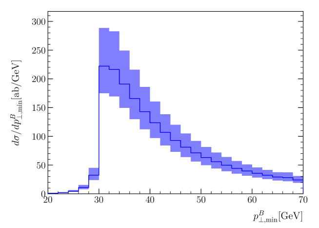
Figure 1: The distribution of the minimum transverse momentum of jets used in the matching, $p^{B}_{\perp,\mathrm{min}}$, for Higgs boson plus dijet production of transverse momenta larger than 30 GeV. The fact that the distribution falls off quickly below the jet analysis scale ensures the resummation phase space with a given minimum jet transverse momentum is covered by a fixed-order generation with a slightly smaller requirement on the jet transverse momentum. For example, a generation of fixed-order events with a minimum jet transverse momentum of 20 GeV is sufficient for an analysis requiring a transverse momentum of at least 30 GeV.

While Eq. (2.1) is mathematically equivalent to Eq. (1), it does not prove that the approach is viable. The first challenge is to ensure that in fact, the integration over the matching, or fixed-order phase space, in the first line of Eq. (2.1) does not actually extend to zero transverse momentum of the matching jets. This would lead to a divergence in the fixed-order cross section and invalidate the starting point. In Fig. 1 we investigate the minimum transverse momentum of jets used in the matching for the evaluation of fixed-order matrix elements. The plot shows $d\sigma/dp^{B}_{\perp,\mathrm{min}}$, where $p^{B}_{\perp,\mathrm{min}}$ is the minimum jet transverse momentum used in the merging with matrix elements (i.e. the minimum transverse momentum in the resulting on-shell Born level kinematics after reshuffling) for Higgs-boson production in association with at least two jets with transverse momentum of at least 30 GeV. One sees that the matrix element sample needs to include events with a minimum jet transverse momentum below the final analysis scale — but not too far below. It is observed that this distribution gets broader, and that the weight for small $p^{B}_{\perp,\mathrm{min}}$ is relatively more important, both for larger rapidity spans, and if more hard jets are required (obviously these two requirements are linked).

The next challenge is to generate all resummation kinematics corresponding to a specific fixed-order or matching kinematics. This is not an obvious switch to make: substituting a requirement on (N)LO kinematics to result in a given Born level jet configuration with that of the full resummation event resulting in a given Born level jet kinematics. The formalism will though be much more computationally efficient, since the fixed-order matrix element is evaluated only once for each fixed-order kinematic point. And furthermore, statistical convergence can be ensured first at the fixed-order stage, before resummation is attempted.

2.2 Phase Space Generation

In order to perform the resummation, we are tasked with the numerical evaluation of the last four lines of Eq. (2.1). In principle, we have to integrate over the phase space of arbitrarily many further real emissions. This is made feasible by the fact that for a given fixed-order configuration with finite rapidity span, only a limited number of additional gluons actually lead to a non-negligible contribution in the resummation. Still, the typical multiplicities in the interesting region of large rapidity separations will be quite high and we are required to inspect the corresponding high-dimensional phase space carefully for an efficient integration. In the following, we discuss how to construct an efficient importance sampling.

2.2.1 Gluon Multiplicity

The typical number of extra emissions depends strongly on the rapidity span of the underlying fixed-order event. Let us, for example, consider a fixed-order FKL-type multi-jet configuration with rapidities $y_{j_{f}},\,y_{j_{b}}$ of the most forward and backward jets, respectively. By construction of the matching algorithm of Ref.[19], the jet multiplicity and the rapidity of each jet are conserved when adding resummation. This implies that additional hard radiation is restricted to rapidities $y$ within a region $y_{j_{b}}\lesssim y\lesssim y_{j_{f}}$. Within HEJ, we require the most forward and most backward emissions to be hard in order to avoid divergences [19], so this constraint in fact applies to all additional radiation.

To simplify the remaining discussion, let us remove the FKL rapidity ordering

$$\mathbf{T}_{y}\prod_{i=1}^{n}\int\frac{\mathrm{d}y_{i}}{2}=\frac{1}{n!}\prod_{i=1}^{n}\int\frac{\mathrm{d}y_{i}}{2}\,,$$ (6)

where all rapidity integrals now cover a region which is approximately bounded by $y_{j_{b}}$ and $y_{j_{f}}$. Each of the $m$ jets has to contain at least one parton; selecting random emissions we can rewrite the phase space integrals as

$$\frac{1}{n!}\prod_{i=1}^{n}\int[\mathrm{d}p_{i}]=\left(\prod_{i=1}^{m}\int[\mathrm{d}p_{i}]\ {\cal J}_{i}(p_{i})\right)\frac{1}{n_{g}!}\prod_{i=m+1}^{m+n_{g}}\int[\mathrm{d}p_{i}]$$ (7)

with jet selection functions

$${\cal J}_{i}(p)=\begin{cases}1&p\text{ clustered into jet }i\\ 0&\text{otherwise}\end{cases}$$ (8)

and $n_{g}\equiv n-m$. Here and in the following we use the short-hand notation $[\mathrm{d}p_{i}]$ to denote the phase-space measure for parton $i$. As is evident from Eq. (7), adding an extra emission $n_{g}+1$ introduces a suppression factor $\tfrac{1}{n_{g}+1}$. However, the additional phase space integral also results in an enhancement proportional to $\Delta y_{j_{f}j_{b}}=y_{j_{f}}-y_{j_{b}}$. This is a result of the rapidity-independence of the MRK limit of the integrand, consisting of the matrix elements divided by the flux factor. Indeed, we observe that the typical number of gluon emissions is to a good approximation proportional to the rapidity separation and the phase space integral is dominated by events with $n_{g}\approx\Delta y_{j_{f}j_{b}}$.

For the actual phase space sampling, we assume a Poisson distribution and extract the mean number of gluon emissions in different rapidity bins and fit the results to a linear function in $\Delta y_{j_{f}j_{b}}$, finding a coefficient of $0.975$ for the inclusive production of a Higgs boson with two jets. In Figs. 2 and 3 we compare the fit with the actual outcome.

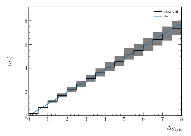
Figure 2: Average number of additional gluon emissions $n_{g}$ as a function of the rapidity span between the extremal jets. The bin entries show the observed numbers in the production of a Higgs boson in association with at least two jets. The solid line shows the function used for the phase space generation.

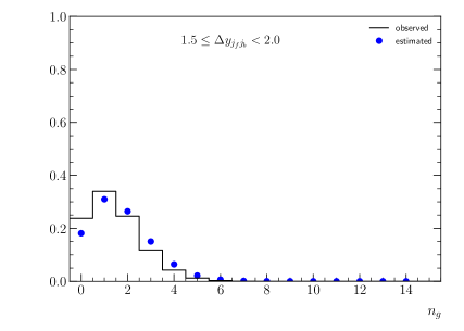
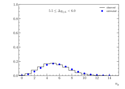
Figure 3: Number of additional gluon emissions $n_{g}$ for two different rapidity spans between the extremal jets. The estimates are based on Poisson distributions with mean values taken from the fit function in Fig. 2 for $\Delta y_{j_{f}j_{b}}=1.75$ and $\Delta y_{j_{f}j_{b}}=5.75$.

2.2.2 Number of Gluons inside Jets

For each of the $n_{g}$ gluon emissions we can split the phase-space integral into a (disconnected) region inside the jets and a remainder:

$$\int[\mathrm{d}p_{i}]=\int[\mathrm{d}p_{i}]\,\theta\bigg{(}\sum_{j=1}^{m}{\cal J}_{j}(p_{i})\bigg{)}+\int[\mathrm{d}p_{i}]\,\bigg{[}1-\theta\bigg{(}\sum_{j=1}^{m}{\cal J}_{j}(p_{i})\bigg{)}\bigg{]}\,.$$ (9)

We choose an importance sampling which is flat in the plane spanned by the azimuthal angle $\phi$ and the rapidity $y$. This is observed in BFKL and valid in the limit of Multi-Regge-Kinematics (MRK). Furthermore, we assume anti-$k_{t}$ jets, which cover an area of $\pi R^{2}$ [24].

In principle, the total accessible area in the $y$-$\phi$ plane is given by $2\pi\Delta y_{fb}$, where $\Delta y_{fb}\geq\Delta y_{j_{f}j_{b}}$ is the a priori unknown rapidity separation between the most forward and backward partons. In most cases the extremal jets consist of single partons, so that $\Delta y_{fb}=\Delta y_{j_{f}j_{b}}$. For the less common case of two partons forming a jet we observe a maximum distance of $R$ between the constituents and the jet centre. In rare cases jets have more than two constituents. Empirically, they are always within a distance of $\tfrac{5}{3}R$ to the centre of the jet [25], so $\Delta y_{fb}\leq\Delta y_{j_{f}j_{b}}+\tfrac{10}{3}R$. In practice, the extremal partons are required to carry a large fraction of the jet transverse momentum (cf. section 2) and will therefore be much closer to the jet axis.

In summary, for sufficiently large rapidity separations we can use the approximation $\Delta y_{fb}\approx\Delta y_{j_{f}j_{b}}$. If there is no overlap between jets, the probability $p_{\cal J,>}$ for an extra gluon to end up inside a jet is then given by (cf. Fig. 4)

$$p_{\cal J,>}=\frac{(m-1)\*R^{2}}{2\Delta y_{j_{f}j_{b}}}\,.$$ (10)

For a very small rapidity separation, Eq. (10) obviously overestimates the true probability. The maximum phase space covered by jets in the limit of a vanishing rapidity distance between all partons is $2mR\Delta y_{fb}$. We therefore estimate the probability for a parton to end up inside a jet as

$$p_{\cal J}=\min\bigg{(}\frac{(m-1)\*R^{2}}{2\Delta y_{j_{f}j_{b}}},\frac{mR}{\pi}\bigg{)}\,.$$ (11)

In Fig. 5 we compare this estimate with the actually observed fraction of additional emissions into jets. We observe good agreement over the whole rapidity range and for different jet multiplicities.

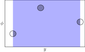
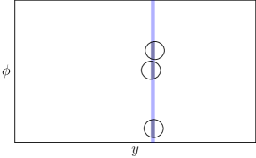
Figure 4: Estimated phase space areas for the emission of extra gluons for sample three-jet configurations. The left panel shows the case of a large rapidity separation. On the right we illustrate the estimate for a very small rapidity span.

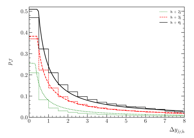
Figure 5: Estimated probability for an extra emission to end up inside a jet compared to the fraction observed in the exclusive production of a Higgs boson with two (green dotted line), three (red dashed line), and four (black solid line) jets.

2.2.3 Gluons outside Jets and Observed Jet Momenta

Using our estimate for the probability of a gluon to be a jet constituent, we arrive at a number $n_{g,{\cal J}}$ of gluons inside jets. Before integrating over their remaining phase space, we first have to determine the momenta $p_{{\cal J}_{i}}$ of the observed (resummation) jets from Eq. (5). To this end, we have to determine the total transverse momentum $\mathbf{q}_{\perp}$ of the gluons outside jets. After generating soft transverse momenta for these $n_{g}-n_{g,{\cal J}}$ gluons, we solve the nonlinear system Eq. (5) using GSL routines [26]. Note that we have to postpone the rapidity integration, since at this point the rapidity span in the phase space integral is not yet known. The most forward and backward partons have to be part of the extremal jets. Therefore, their momenta will only be determined in the next step.

2.2.4 Gluons inside Jets

Recall that after the first step in the phase space parametrisation, Eq. (7), each jet has exactly one constituent. We now assign each of the $n_{g,{\cal J}}$ gluons to a random jet. For jets with a single constituent, the parton momentum is fixed completely by the constraints in Eq. (2.1). In the case of two constituents, we observe that the partons are always inside the jet cone with radius $R$ and often very close to the jet centre. This allows an efficient integration by choosing a distance to the jet centre and an azimuthal angle with respect to the jet axis for one of the partons, which determines all momentum components of both constituents.

As is evident from Fig. 5, jets with three or more constituents are rare and an efficient phase-space sampling is less important. For such jets, we exploit the observation that partons with a distance larger than $R_{\text{max}}=\tfrac{5}{3}R$ [25] to the jet centre are never clustered into the jet. Assuming $N$ constituents, we choose distances, angles, and transverse momenta for $N-1$ of them and determine the momentum of the last constituent from the requirement that the constituent momenta have to add up to the jet momentum. Since this last momentum may lie outside the jet cone, it is mandatory to check explicitly whether all candidates are actually clustered into the considered jet. This is to ensure the correct coverage of phase space.

After constructing the resummation jets, we are now in the position to evaluate the rapidity integrals for the partons outside the jets. Finally, we use fastjet [27] to recluster all emitted partons into jets again to check whether the reshuffling conditions imposed by Eq. (2.1) are fulfilled. We also ensure that all partons are assigned as intended, i.e. the $n_{g,{\cal J}}$ designated jet constituents are indeed part of their respective jet and all remaining partons end up outside jets.

We have now outlined the practical steps necessary to implement the rewritten formula of Eq. (2.1). In the following section we discuss the results obtained with the new formalism in the key process of Higgs boson production in association with at least two jets. Firstly we confirm that if we limit ourselves to matching with fixed order samples with up to three jets that we reproduce the results obtained with the previous formalism, but now with a much higher efficiency. We will then show and discuss the impact of now being able to increase the multiplicity in the fixed order samples and also compare our results to fixed-order next-to-leading order predictions.

3 Results

The matching procedure described in this work is significantly more efficient and flexible than the approach used in previous versions of HEJ. To illustrate this, we present new results for the production of a Higgs boson in association with at least two jets matched to leading-order events with up to four jets. Previously, matching of HEJ to just three jets was achieved for this process, while using significantly more CPU resources than necessary with the current approach. In its new formulation, the matching is in practice only limited by the capabilities of the underlying fixed-order generator. For instance, the generation of one set of $1000$ unweighted leading-order events for the production of a Higgs boson with four jets typically took a few CPU days using MadGraph5_aMC@NLO [28]. It is then just a few additional CPU seconds to generate $100$ resummation events from each of the fixed-order 4-jet events, so $100\,000$ trial resummation configurations in total. In the previous matching approach, generating $100\,000$ resummation configurations would require the same number of fixed-order matrix element evaluations. In this sense the new matching algorithm is more efficient by a factor of almost 100.

This section will present the results obtained with the new procedure for matching and resummation. Section 3.1 describes the cuts and analysis used. Section 3.2 compares new results with matching up to three jets with those obtained previously, and demonstrates that the two methods yield equivalent results. Section 3.3 investigates the stability of the results obtained by investigating the impact of increasing the order to which matching is achieved. In general, the matching to higher multiplicities should have little impact for configurations where the four-jet contribution is insignificant or the approximation within HEJ already provides a good description. Conversely, the corrections from matching to successive multiplicities can serve to indicate the stability of the HEJ predictions for observables sensitive to additional hard radiation. Finally, in Section 3.4 we match the inclusive $Hjj$-cross section to NLO accuracy, thus obtaining the most precise predictions for $Hjj$-production, including the effects of VBF cuts and central jet vetos. These results are compared to those obtained at fixed next-to-leading order accuracy.

3.1 Setup

To facilitate the comparison with previous results we will adopt the cuts of the experimental analysis of Ref. [29], and the parameters of our analysis in Ref. [18]. To recapitulate, we consider the gluon-fusion-induced production of a Higgs boson together with at least two anti-$k_{t}$ jets with transverse momenta $p_{\perp,j}>30\,$GeV, rapidities $|y_{j}|<4.4$, and radii $R=0.4$ at the $13\,$TeV LHC. While it is obviously irrelevant for the considerations of the QCD corrections considered in this paper, we consider the Higgs boson decay into two photons with

$$|y_{\gamma}| <2.37,\qquad 105~{}\textrm{GeV}<m_{\gamma_{1}\gamma_{2}}<160~{}\textrm{GeV},$$

$$p_{\perp,\gamma_{1}} >0.35\,m_{\gamma_{1}\gamma_{2}},\qquad p_{\perp,\gamma_{2}}>0.25\,m_{\gamma_{1}\gamma_{2}},$$ (12)

and separations $\Delta R(\gamma,j),\Delta R(\gamma_{1},\gamma_{2})>0.4$ from the jets and each other. To be consistent with our previous analysis we set the Higgs-boson mass to $m_{H}=125\,$GeV, a width of $\Gamma_{H}=4.165\,$MeV and a branching fraction of $0.236\%$ for the decay into two photons. We use the CT14nlo PDF set [30] as provided by LHAPDF6 [31].

In addition to inclusive quantities with the basic cuts listed above, we also consider additional VBF-selection cuts applied to the hardest jets as in [29]:

$$|y_{j_{1}}-y_{j_{2}}|>2.8,\qquad m_{j_{1}j_{2}}>400~{}\textrm{GeV}.$$ (13)

In the first step, we generate leading-order events with two, three and four jets. With our new matching procedure we are free to use an arbitrary fixed-order event generator for this purpose. For the present analysis we employ version 2.5.5 of MadGraph5_aMC@NLO [28]. For each jet multiplicity we produce about 2000 sets of unweighted events, each comprising 10 000 events for the sets with two or three jets and 1000 events for sets with four jets.

As the transverse momenta of the jets are modified during resummation (cf. Eq. (5)), we have to generate at least a fraction of events with Born-jet momenta below the threshold of $30\,$GeV required from the observed jets. As already shown in Fig. 1 the contribution after the resummation from such tree-level configurations in the matching drops off very rapidly below the jet transverse momentum analysis scale of $30\,$GeV. Passing this information to the underlying fixed-order generator, such that only a small fraction of events are generated below the nominal transverse momentum threshold could improve the sampling considerably. Having such an option would therefore be highly desirable. For the time being, we manually generate 200 additional sets of Born-level events with transverse momenta down to $20\,$GeV for each jet multiplicity.

Events with more exclusive jets than can be reasonably evaluated in MadGraph5_aMC@NLO are unmatched and generated with a custom built Monte Carlo generator based on tree-level HEJ matrix elements instead of full leading-order ones. In this way, we can supplement the fixed-order input with events including up to ten jets obtained within the HEJ approximation. These events are simply passed through the same matching mechanism based on Eq. (2.1) just as the lower-multiplicity events obtained using MadGraph5_aMC@NLO. The maximum multiplicity of ten is an arbitrary cut-off, based on an explicit check that the impact on observables at this multiplicity is negligible.

Since the final kinematics required for a kinematic scale setting are not known at the point of generating fixed-order events, we use a fixed renormalisation and factorisation scale of $\mu_{r}=\mu_{f}=m_{H}$ during the fixed-order generation. After resummation the events are rescaled to a central scale of $\mu_{r}=\mu_{f}=H_{T}/2$. In order to assess the scale dependence, we independently vary both the renormalisation and factorisation scales by factors $\{1/2,1/\sqrt{2},1,\sqrt{2},2\}$ and discard combinations with $\mu_{r}/\mu_{f}<1/2$ or $\mu_{r}/\mu_{f}>2$. In the effective Higgs-gluon coupling, we keep the renormalisation scale at the Higgs-boson mass and apply the limit of an infinite top-quark mass. These scale settings and even the use of the infinite top-mass limit are however not inherent to the use of the high-energy resummation of HEJ, but can be included with modified components of the amplitudes, similar to Ref. [32].

After generating the tree-level input events, we apply resummation as presented in the previous sections. Recent progress described in [18] allows us to apply resummation not just for FKL-ordered matching-events, but also the sub-leading contribution from events with three jets or more, where the rapidity-ordering of the two most forward or most backward jets is flipped compared to FKL ordering. This corresponds to a gluon emission outside a rapidity-interval delimited by quark jets. For each resummation-type tree-level event, we generate 100 trial configurations in the resummation phase space. For the remaining sub-leading events we cannot add resummation and simply adjust the factorisation and renormalisation scales as described above.

3.2 Comparison to previous results

In order to demonstrate the validity of the new approach we compare here first our results with leading-order matching up to three jets to those obtained in our previous work [18] . We find good agreement within the statistical errors. As examples, we show the transverse momentum distributions for the Higgs boson for inclusive and VBF cuts in Fig. 6. The previous and new method of organising the calculation are equivalent. For the comparison, we have adjusted our settings to match those in [18] as closely as possible. Apart from restricting the fixed-order matching to configurations with at most three jets, this also means that the extremal partons are required to have a fixed minimum transverse momentum of $27\,$GeV instead of a fraction of the corresponding jet momentum, as discussed in section 2.

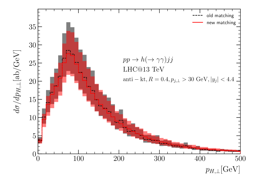
(a)

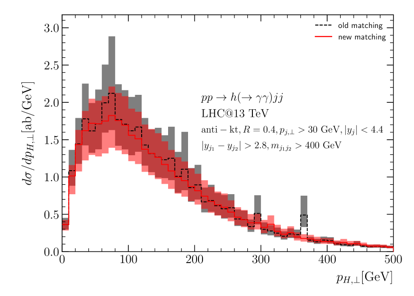
(b)

Figure 6: Comparison of the new matching procedure to previous HEJ results obtained in [18]. The panels show the transverse momentum distributions of the Higgs boson for (a) inclusive cuts and (b) VBF cuts.

3.3 Impact of four-jet matching on Distributions

The HEJ approximation is exact in the limit of Multi-Regge kinematics, i.e. for large rapidity separation between hard jets. An equivalent characterisation is to demand the centre-of-mass energy and the invariant masses between all final-state jets to be much larger than the typical transverse momenta of these. If these conditions are fulfilled, we expect a good HEJ prediction and hence small matching corrections. In order to assess the perturbative stability of the final predictions, we will here study the impact on the resummed and matched cross section of scale variations and of successive matching to two-jet, three-jet and four-jet tree-level events.

One of the main goals of HEJ is to improve the prediction of the gluon-fusion background to Higgs-boson production in weak-boson fusion. Standard VBF cuts project out a kinematic region with a large invariant mass between the hardest jets, where the gluon fusion receives significant contributions from higher jet multiplicities. Fig. 7(a) displays the relative contribution of the exclusive two-, three- and four-jet component to the distribution on the invariant mass between the two hardest (in transverse momentum) jets. The relative contribution from exclusive three- and four-jet-events increases with increasing $m_{{j_{1}}{j_{2}}}$. Fig. 7(b) displays the impact of matching of successive multiplicity on the distribution of the invariant mass between the two hardest (in transverse momentum) jets. The effect of the four-jet matching is small but non-zero even at large $m_{j_{1}j_{2}}$. This is because even in this limit a large separation between all jets is not guaranteed.

The contribution from jet multiplicities of more than or equal to 5 is less than $5\%$ for an invariant mass of at least $1\,$TeV. We conclude that the uncertainty on the distribution of $m_{{j_{1}}{j_{2}}}$ from terminating the matching at the four-jet contribution is insignificant, and well within the quoted scale variation.

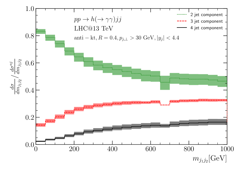
(a)

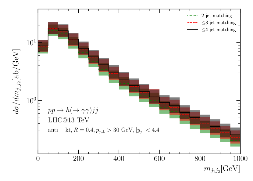
(b)

Figure 7: Distribution of the invariant mass between the hardest jets. Panel (a) shows the fractional contributions from exclusive two-, three-, and four-jet events. Panel (b) depicts the effects of fixed-order matching up to two, three, and four jets.

A central prediction of BFKL, which arises also within HEJ, is a linear increase in the number of jets for a growing rapidity span between the most backward and forward jets. This behaviour is demonstrated in Fig. 8, which also investigates the impact of matching to tree-level of successive multiplicities. Although the contribution from higher jet multiplicities increases with the rapidity separation, the effect of fixed-order matching on this observable actually decreases. This confirms our expectation that the HEJ approximation works well for large $\Delta y_{j_{f},j_{b}}$. It is this linear increase in the average number of jets versus increasing rapidity span which can be exploited to suppress the gluon-fusion contribution with a central jet veto.

In contrast to this, if the two hardest jets are tagged, and only jets in-between these are counted as a function of the rapidity difference between the hardest jets, then the initial linear growth stalls at an average number of jets of around 2.3. The difference in behaviour to the VBF contribution is therefore less pronounced by tagging the hardest jets, rather than the most forward and backward hard jets. This was investigated further in Ref.[33]. Also, the impact of the matching corrections remains sizeable for all rapidity separations.

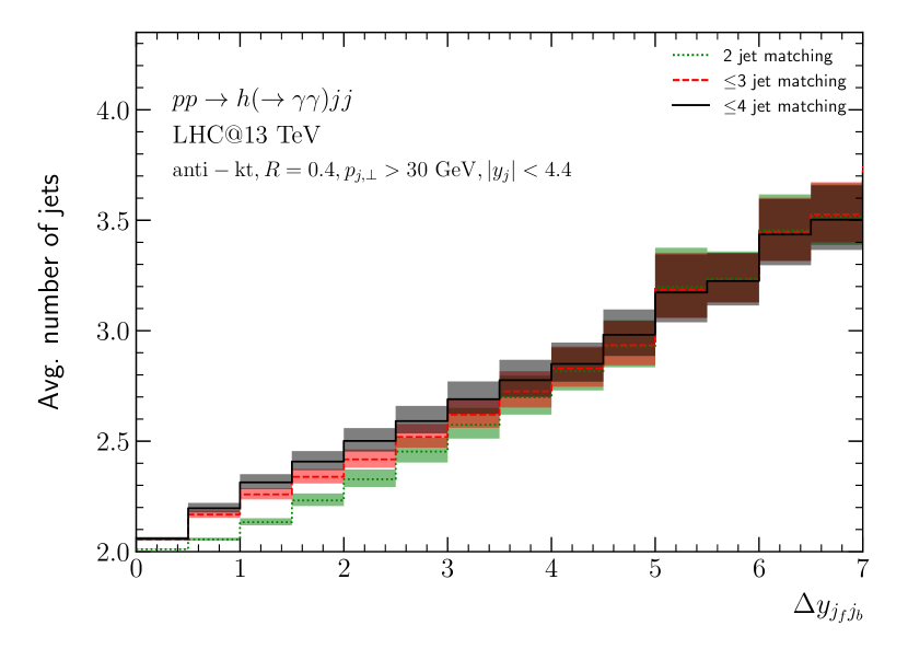
(a)

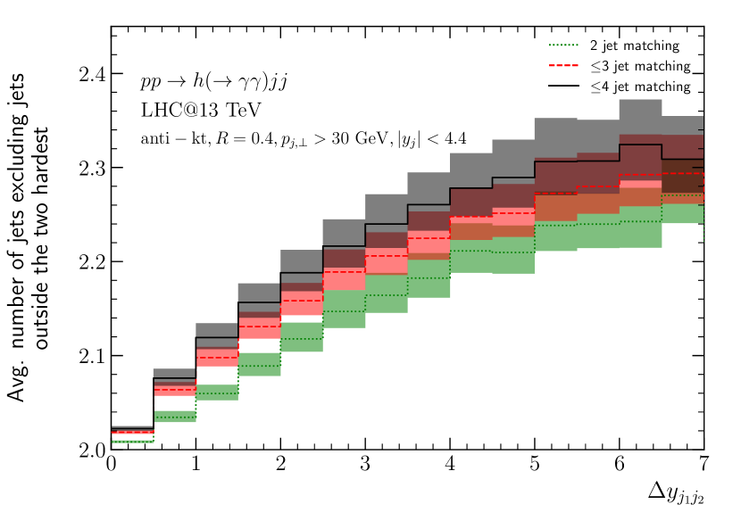
(b)

Figure 8: Average number of jets for fixed-order matching up to two, three, and four jets. In (a) we show the average total number of jets vs. the maximum rapidity-separation. In (b) we show the number of jets in the rapidity region of the two hardest jets.

In observables which are neither dominated by higher jet multiplicities nor completely described by the HEJ approximation we observe that the matching corrections are converging, but the corrections from four-jet matching are non-negligible. In Fig. 9 we show the distribution of the Higgs-boson transverse momentum with inclusive and with VBF cuts. While there is a notable difference between the matching to fixed-order predictions up to two and three jets, the effect of four-jet matching is much smaller. In all cases the matching corrections are well inside the scale variation.

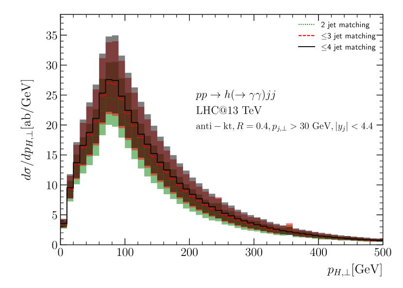
(a)

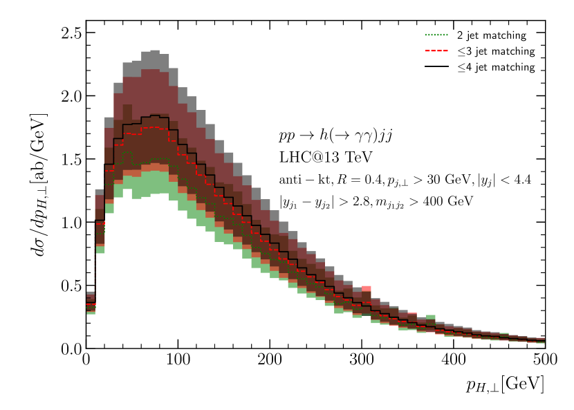
(b)

Figure 9: Distribution of the Higgs-boson transverse momentum with (a) inclusive and (b) VBF cuts.

The azimuthal angle between jets is of particular interest for the extraction of the $CP$-properties of the effective coupling between the Higgs boson and gluons. Fig. 10 shows the effects of fixed-order matching on the distribution of the angle between the two hardest jets. Similar to the transverse momentum distribution in Fig. 9 the corrections from four-jet matching are uniformly moderate.

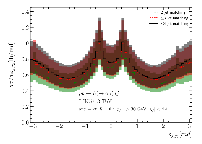
(a)

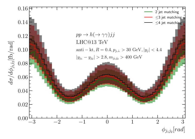
(b)

Figure 10: Distribution of the azimuthal angle between the two hardest jets with (a) inclusive and (b) VBF cuts.

In order to achieve a greater reduction of the gluon-fusion background to weak-boson fusion within the VBF-cuts, a veto on further jets can be applied. This has the added benefit of reducing the contribution from higher jet multiplicities, which is harder to predict in perturbation theory. The effectiveness of such a cut relies on the difference in the quantum corrections to the processes of VBF and GF[11]. Since this difference is due to the $t$-channel colour-octet exchange of the GF process, we will apply a central jet veto only in the regions away from the tagging jets, since the collinear regions have similar emissions in VBF and GF. This is a slight improvement on the normal central jet veto cuts, and is inspired by the Zeppenfeld variable[34]. Here, we consider a veto of events with jets within a rapidity distance $y_{c}$ to the rapidity centre of either (a) most forward and backward jets or (b) the hardest jets (see also [34, 33]). In case (b), we only consider vetoing on further jets which are in between the two hardest jets. The results are shown in Fig. 11. As expected, the cross section in case (a) converges for large $y_{c}$ to the exclusive prediction for the production of a Higgs boson with exactly two jets, irrespective of the fixed-order matching to higher multiplicities. When applying the jet veto between the hardest jets in case (b), the overall reduction in the GF component is much smaller, and insignificant compared to the scale variation.

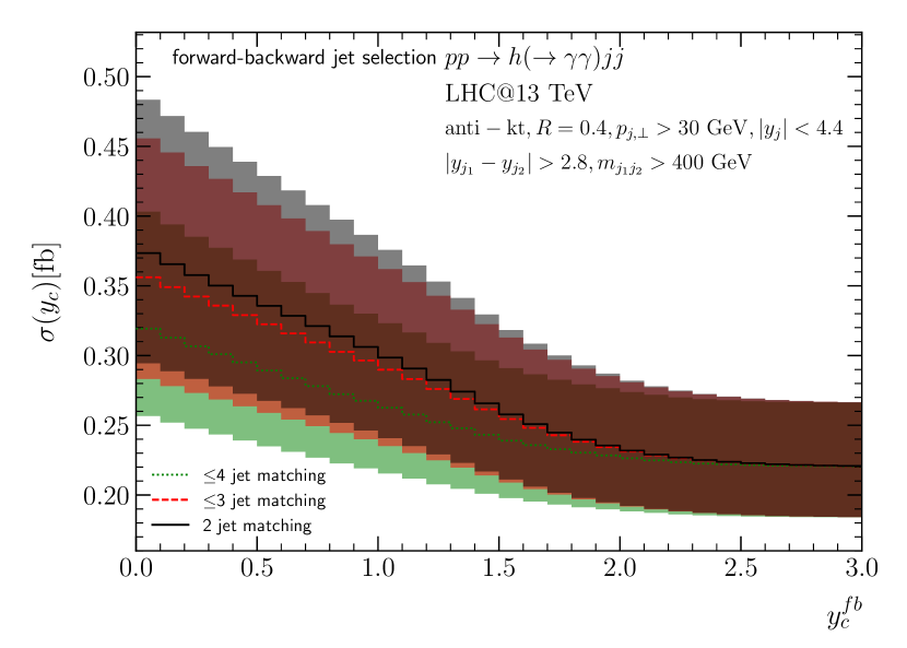
(a)

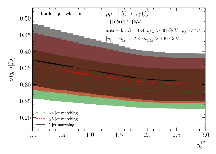
(b)

Figure 11: Effect of a jet veto between (a) the most forward and backward jets and (b) the two hardest jets. Events with additional jets within a distance of $y_{c}$ to the rapidity centre are discarded.

3.4 Matching and Comparison to Fixed Next-to-Leading Order

The complete reformulation of the formalism for matching and all-order summation described in Sec. 2 has allowed for matching to higher jet multiplicities in HEJ. The impact of the four-jet matching on the studied distributions is small. The method presented in the earlier sections has been concerned with a point-by-point matching of the resummation to full high-multiplicity tree-level accuracy. As extensively demonstrated in Section 3.3, this achieves perturbatively stable results for the shapes of distributions. In order to reduce the scale variation and benefit from the full NLO results for $Hjj$-production, we will now rescale the results for HEJ within the inclusive cuts of Eq. (3.1) to the NLO cross section for each choice of factorisation and renormalisation scale. Thereby, full NLO accuracy is obtained for all dijet observables, LO accuracy for trijet observables, and the impact on the shape of distributions from four-jet contributions is accounted for at LO. This method was applied also in Ref.[33]. While this approach does not change the shape of distributions, the scale variation is reduced to the level of NLO predictions.

We will here compare these predictions to those obtained at fixed NLO using MCFM [35, 36] and SHERPA [5].

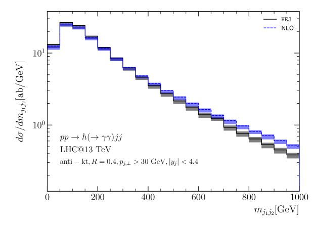
Figure 12: Distribution of the invariant mass between the two hardest jets. The HEJ result with fixed-order matching up to 4 jets is shown by the solid black line. The MCFM NLO prediction corresponds to the dashed blue line. The central renormalisation and factorisation scale is set to $H_{T}/2$, and they are varied independently by a factor of two.

Fig. 12 compares the predictions for the distribution on the invariant mass between the two hardest jets. The scale variation on the HEJ results is vastly reduced to that of Fig. 7, as generally expected by the inclusion of the full NLO corrections. The distribution obtained with HEJ for the invariant mass between the two hardest (in transverse momentum) jets is still significantly steeper than that at pure NLO, as a result of the possibility of significantly higher jet multiplicity, and the fact that hard central jets have a slightly smaller PDF-suppression than hard forward jets, and therefore the two hardest jets tend to also be central. This means that the prediction for the cross section within the VBF cuts is significantly smaller with HEJ than for NLO, and indeed lies outside the scale-variation band obtained at NLO.

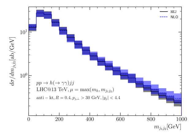
Figure 13: Distribution of the invariant mass between the two hardest jets, for a central scale choice of $m_{j_{1}j_{2}}$. The HEJ result with fixed-order matching up to 4 jets is shown by the solid black line. The SHERPA NLO prediction corresponds to the dashed blue line.

In numbers, the cross sections obtained (at NLO) for $pp\to h(\to\gamma\gamma)jj$ for inclusive cuts and with a central scale choice of $\mu_{r}=\mu_{f}=H_{T}/2$ is $6.58^{+0.08}_{-0.57}$ fb. This is obviously the same as that obtained with HEJ for inclusive cuts, once the cross sections are normalised to NLO accuracy. For the VBF cuts, the NLO cross section is $0.872^{+0.024}_{-0.090}$ fb, and that obtained for HEJ is $0.561^{+0.031}_{-0.067}$ fb. Even though the inclusive cross section for HEJ is normalised to that obtained at NLO, a sizeable difference in the cross section within the VBF cuts arises due to a difference in the slope of distribution in $m_{j_{1}j_{2}}$ and the requirement of $m_{j_{1}j_{2}}>400$ GeV for the VBF cuts. The VBF cuts cause a similar reduction in the cross section to $13.2\%$ (NLO) and $8.5\%$ (HEJ) of the inclusive cross section respectively.

Comparing the results of Fig. 12 and Fig. 13 we observe that a choice of a central scale for the NLO calculation of $\mu_{r}=\mu_{f}=H_{T}/2$ leads to a suspiciously small scale variation - and indeed the central scale choice gives results close to the extremum obtained with the variations, despite the scales being varied either side of the central choice of $\mu_{r}=\mu_{f}=H_{T}/2$. Such a behaviour of the scale variation often indicates that the NLO scale variation obtained with this scale choice is underestimating the theoretical uncertainty[37].

Indeed, Ref.[37] investigated the distribution in $m_{j_{1}j_{2}}$ for dijet production at NNLO at the LHC, and found that at large $m_{j_{1}j_{2}}$ this scale choice is favoured over $p_{T}$ based on perturbative convergence. The invariant mass between the two hardest jets obviously is not a stable perturbative scale choice for all bins in the distribution, which extends to very low values of $m_{j_{1}j_{2}}$. With a central scale choice of $\mu_{f}=\mu_{r}=\max(m_{h},m_{j_{1}j_{2}})$, the central scale choice leads to predictions in the centre of the variation band. The scale variation bands obtained with NLO and HEJ also overlaps in each bin of the distribution. With this central scale choice, the cross sections obtained at NLO for inclusive cuts is $6.23^{+1.11}_{-1.22}$ fb. For the VBF cuts, the NLO cross section is $0.542^{+0.156}_{-0.125}$ fb, and that obtained for HEJ is $0.359^{+0.045}_{-0.061}$ fb. The VBF cuts cause a similar reduction in the cross section to 8.7% (NLO) and 5.8% (HEJ) of the inclusive cross section respectively.

It is worth noting that (ignoring the mass of each jet) since $m^{2}_{j_{1}j_{2}}=2p_{\perp j_{1}}p_{\perp j_{2}}(\cosh(y_{j_{1}}-y_{j_{2}})-\cos(\phi_{j_{1}}-\phi_{j_{2}}))$ a central scale choice of $\mu_{r}=m_{j_{1}j_{2}}$ systematically runs $\alpha_{s}$ such that $\alpha_{s}\Delta y_{j_{1}j_{2}}$ tends to a constant for large $\Delta y_{j_{1}j_{2}}$. This would seem to spoil the standard argument of BFKL noting large and systematic leading logarithmic corrections of the form $(\alpha_{s}\Delta y_{j_{f}j_{b}})^{k}$ at large $\Delta y_{j_{f}j_{b}}$, at least for $\Delta y_{j_{1}j_{2}}$ sufficiently large that $m_{j_{1}j_{2}}$ is close to the hadronic collision energy that only two jets exists, because hard radiation beyond the two jets required is suppressed. For events with more than two jets, there is no direct correlation between $\Delta y_{j_{1}j_{2}}$ and $\Delta y_{j_{f}j_{b}}$. The results for the scale choice of $\mu_{r}=\mu_{f}=m_{j_{1}j_{2}}$ are discussed further in appendix A. Here we just note that the apparent convergence of the perturbative series (i.e. a comparison of the LO and NLO results and scale variation) is not significantly different for the two scale choices. The scale variation around $\mu_{r}=\mu_{f}=H_{T}/2$ is accidentally small, since the central scale choice leads to the maximum cross section within the variation.

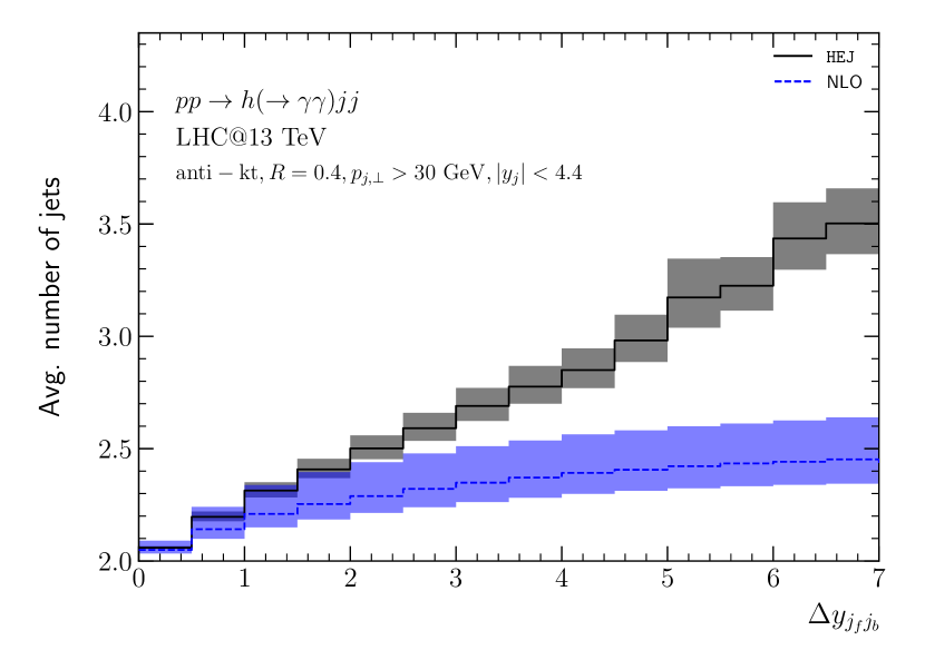
(a)

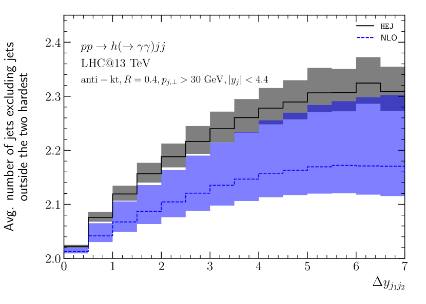
(b)

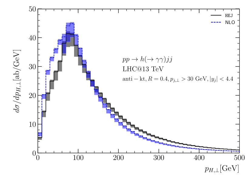
(c)

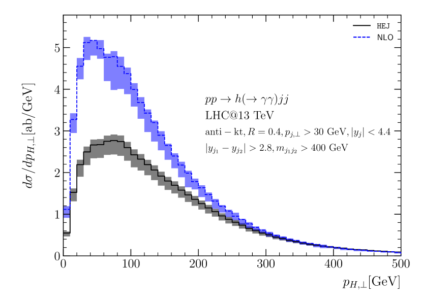
(d)

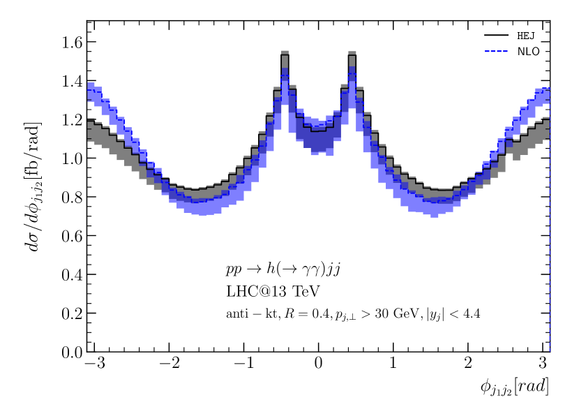
(e)

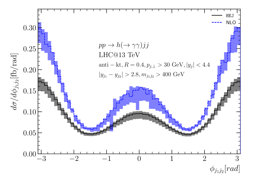
(f)

Figure 14: Comparison of HEJ results with fixed-order matching up to 4 jets (solid black line) with NLO predictions from MCFM (dashed blue line). The shown observables are (a) the average jet multiplicity, (b) the number of jets in between the two hardest jets, the distribution of the Higgs-boson transverse momentum with (c) inclusive and (d) VBF cuts, and the distribution of the azimuthal angle between the hardest jets with (e) inclusive and (f) VBF cuts.

Fig. 14(a) and Fig. 14(b) investigates the potential for using perturbative corrections in the form of additional jet-radiation as a means of identifying the gluon-fusion production channel. For the same event selection, the figure compares the results for the average number of jets counting additional jets (a) between the most forward and backward jets, and (b) in-between the two hardest jets only. The results on Fig. 14(a) are relevant for e.g. jet vetos between the most forward and most backward hard jet, whereas Fig. 14(b) is relevant if the veto is applied between just the two hardest jets in the event. The results for HEJ are identical to those for 4-jet matching in Fig. 8 (since just the total cross section has been adjusted to the NLO result for $Hjj$), but the results are here compared to those obtained using the NLO calculation for $Hjj$-production. As observed also in previous analyses[38], the results obtained at NLO tends towards 2.5, where the exclusive, hard three-jet cross section is as large as the two-jet cross section. This clearly illustrates the slow convergence of the perturbative series. The results for NLO and for HEJ start diverging already at small $\Delta y_{j_{f}j_{b}}$. It is worth noting that the linear growth in the number of hard jets vs. $\Delta y_{j_{f}j_{b}}$ has been experimentally confirmed[39, 6] for several processes with colour octet exchanges in the $t$-channel.

Even though exactly the same events are involved, the breakdown of the convergence is less obvious in Fig. 14(b). The number of jets in-between the two hardest is obviously smaller, and both the results for HEJ and for NLO appear to asymptote to a value for the average number of jets of 2.2 for NLO and 2.3 for HEJ.

Fig. 14 also shows the predictions for the Higgs transverse momentum spectrum obtained at NLO and with HEJ both for inclusive (c) and VBF-cuts (d). The distributions are very similar for inclusive cuts, with a peak around 80 GeV, and the spectrum from HEJ slightly harder. For VBF cuts, the prediction for HEJ is lower than that for NLO, as a result of the steeper spectrum in $m_{j_{1}j_{2}}$ and the requirement of $m_{j_{1}j_{2}}>400$ GeV. The two predictions for the high-$p_{\perp}$ tail within the VBF cuts coincide, but in this region the infinite top-mass approximation is certainly not trustworthy.

Finally, Fig. 14(c) and (d) compares the azimuthal angle between the two hardest jets for (c) inclusive and (d) VBF cuts respectively. In both the distributions, the region of back-to-back jets at $\phi=\pm\pi$ is slightly suppressed in HEJ compared to NLO. The valley at $\phi=0$ for the inclusive cut is due to the jet-algorithm removing the collinear region. The result within the VBF cuts on Fig. 14(f) show that the reduction in the cross section within the VBF cuts for HEJ compared to NLO predominantly is in the region of back-to-back jets and jets in the same azimuthal direction. The region at $\phi_{j_{1}j_{2}}=0$ is not collinear within the VBF cuts, and so the structure induced by the jet algorithm within the inclusive cuts of Fig. 14(e) is not present within the VBF cuts of Fig. 14(f).

4 Conclusions

We have presented a reformulation of the matching formalism within HEJ, which recasts the calculation as one of merging fixed-order samples of increasing multiplicity. The merging is performed respecting the resummation of perturbative terms logarithmically enhanced at large $\hat{s}/p_{t}^{2}$. While the formalism is mathematically equivalent to that previously used, stable results are obtained using orders of magnitudes less CPU time. This allows matching to be performed to higher multiplicity.

The new formalism was used in a study of Higgs-boson production in association with dijets. The impact of the higher-multiplicity merging is minimal on the shape of distributions important for the application of VBF cuts. For a central scale choice of $\mu_{f}=\mu_{r}=H_{T}/2$, the VBF cuts reduce the inclusive cross section of $6.58^{+0.08}_{-0.57}$ fb on the $h\to\gamma\gamma$-channel to 13% ($0.872^{+0.024}_{-0.090}$ fb) at NLO, or 8.5% ($0.561^{+0.031}_{-0.067}$ fb) once both NLO and the HEJ-corrections are accounted for. The further suppression within HEJ is due to a steeper falling spectrum in the invariant mass between the two hardest jets. The NLO scale dependence is estimated by varying the renormalisation and factorisation scale independently by a factor of two. However, the scale variation around $H_{T}/2$ is artificially small, since the central scale choice achieves a value close to the maximum within the variations. With a scale choice of $\mu_{r}=\mu_{f}=m_{j_{1}j_{2}}$ (but bounded from below by $m_{h}$), the spectrum is similar at NLO and with the further HEJ-corrections. With the scale choice, the inclusive NLO cross section for $h(\to\gamma\gamma)jj$-cross section is $6.23^{+1.11}_{-1.22}$ fb, and $0.542^{+0.156}_{-0.125}$ fb within the VBF cuts. The result for HEJ within the VBF cuts is $0.359^{+0.045}_{-0.061}$ fb. The VBF cuts cause a similar reduction in the cross section to 8.7% (NLO) and 5.8% (HEJ) of the inclusive cross section respectively.

The formalism presented in this report will be instrumental in the further developments, including an account of heavy quark mass effects, and mergings of NLO cross sections.

Appendix A Result for the Central Scale Choice of $m_{j_{1}j_{2}}$

Fig. 15 shows the same distributions for NLO and HEJ (with the inclusive cross section scaled to that of NLO for each scale choice) as those investigated on Fig. 14, but for predictions obtained using a central scale of $\mu_{f}=\mu_{r}=\max(m_{h},m_{j_{1}j_{2}})$. Panel (a) shows the average number of hard jets vs. the rapidity difference between the forward-backward jet pair. The result for NLO is similar to that obtained with the scale $H_{T}/2$, but the NLO scale variation is reduced (even though the scale variation on the NLO cross section themselves is increased by using $m_{j_{1}j_{2}}$ instead of $H_{T}/2$). The rise in the number of hard jets is slightly stronger for HEJ than with the scale of $H_{T}/2$.

Fig. 15(b) shows the average number of jets, counting only additional jets if their rapidity is in-between that of the two hardest jets. The behaviour of the NLO prediction for small $\Delta y_{j_{1}j_{2}}$ is similar to that displayed on Fig. 14(b) until $\Delta y_{j_{1}j_{2}}\sim 3$, after which the average number of jets decreases. This behaviour is a result of the decreasing value of $\alpha_{s}$ for large $\Delta y_{j_{1}j_{2}}$ with this scale choice.

The remaining plots on Fig. 15(c)-(f) all show similar features to those of Fig. 14, but with a smaller cross section and larger scale variation for the results at NLO.

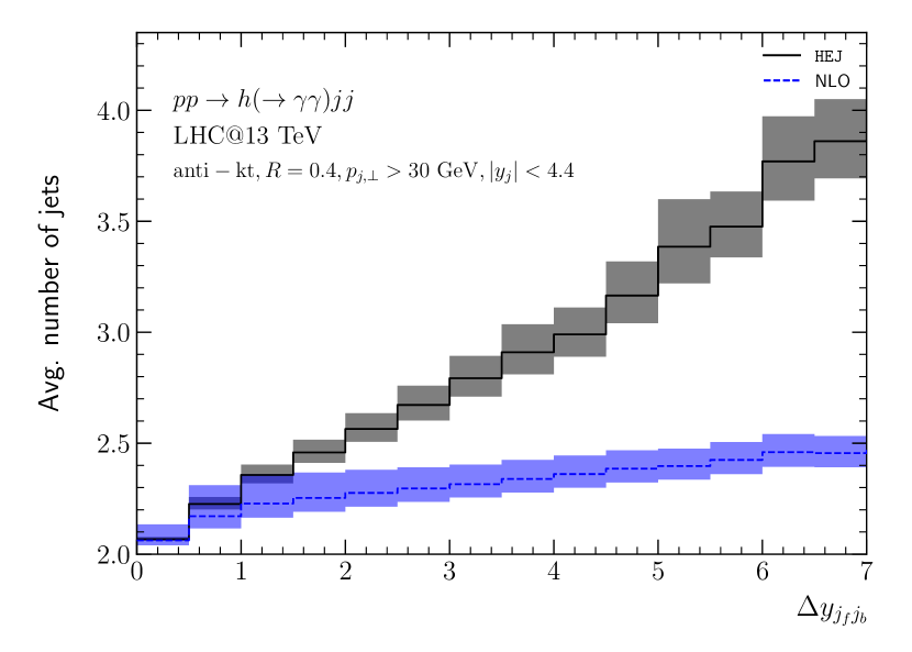
(a)

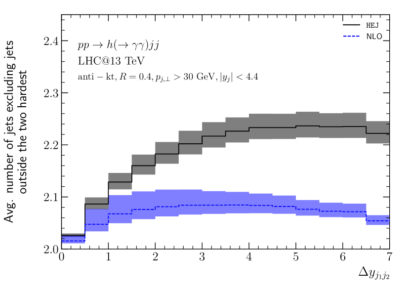
(b)

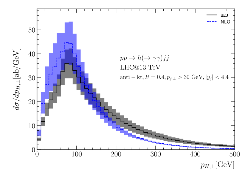
(c)

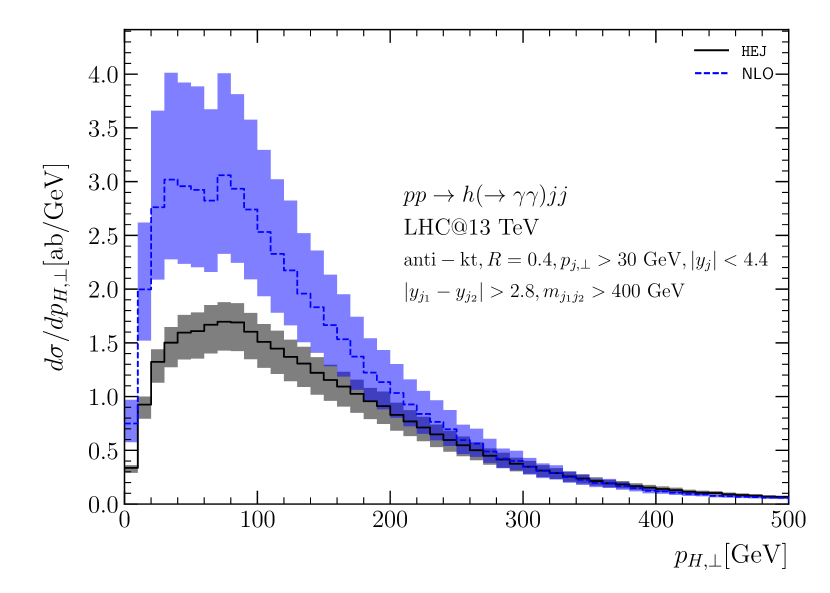
(d)

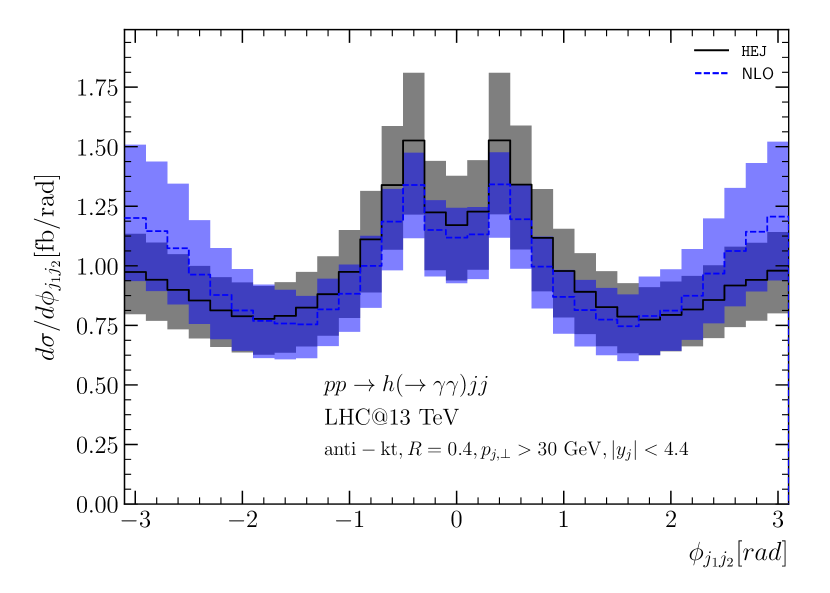
(e)

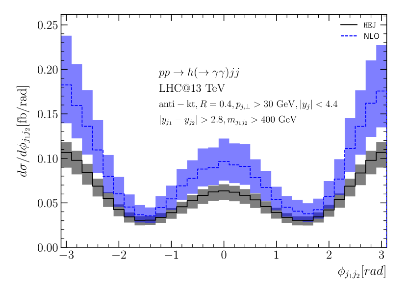
(f)

Figure 15: Comparison of HEJ results with fixed-order matching up to 4 jets (solid black line) with NLO predictions from SHERPA (dashed blue line) for a central scale choice of $\mu_{r}=\mu_{f}=\max(m_{h},m_{j_{1}j_{2}})$. The shown observables are (a) the average jet multiplicity, (b) the number of jets in between the two hardest jets, the distribution of the Higgs-boson transverse momentum with (c) inclusive and (d) VBF cuts, and the distribution of the azimuthal angle between the hardest jets with (e) inclusive and (f) VBF cuts.

References

- [1] M. Dasgupta, F. Dreyer, G. P. Salam and G. Soyez, Small-radius jets to all orders in QCD, JHEP 04 (2015) 039, [1411.5182].
- [2] M. Dasgupta, F. A. Dreyer, G. P. Salam and G. Soyez, Inclusive jet spectrum for small-radius jets, JHEP 06 (2016) 057, [1602.01110].
- [3] J. Bellm et al., Herwig 7.0/Herwig++ 3.0 release note, Eur. Phys. J. C76 (2016) 196, [1512.01178].
- [4] T. Sjöstrand, S. Ask, J. R. Christiansen, R. Corke, N. Desai, P. Ilten et al., An Introduction to PYTHIA 8.2, Comput. Phys. Commun. 191 (2015) 159–177, [1410.3012].
- [5] T. Gleisberg, S. Höche, F. Krauss, M. Sch”onherr, S. Schumann, F. Siegert et al., Event generation with SHERPA 1.1, JHEP 02 (2009) 007, [0811.4622].
- [6] D0 collaboration, V. M. Abazov et al., Studies of boson plus jets production in collisions at TeV, Phys.Rev. D88 (2013) 092001, [1302.6508].
- [7] ATLAS collaboration, G. Aad et al., Measurements of the W production cross sections in association with jets with the ATLAS detector, Eur. Phys. J. C75 (2015) 82, [1409.8639].
- [8] J. R. Andersen, T. Binoth, G. Heinrich and J. M. Smillie, Loop induced interference effects in Higgs Boson plus two jet production at the LHC, JHEP 0802 (2008) 057, [0709.3513].
- [9] A. Bredenstein, K. Hagiwara and B. Jäger, Mixed QCD-electroweak contributions to Higgs-plus-dijet production at the LHC, Phys.Rev. D77 (2008) 073004, [0801.4231].
- [10] L. J. Dixon and Y. Sofianatos, Analytic one-loop amplitudes for a Higgs boson plus four partons, JHEP 0908 (2009) 058, [0906.0008].
- [11] Y. L. Dokshitzer, V. A. Khoze and T. Sjöstrand, Rapidity gaps in Higgs production, Phys.Lett. B274 (1992) 116–121.
- [12] V. S. Fadin, E. A. Kuraev and L. N. Lipatov, On the Pomeranchuk singularity in asymptotically free theories, Phys. Lett. B60 (1975) 50–52.
- [13] E. A. Kuraev, L. N. Lipatov and V. S. Fadin, Multi - Reggeon processes in the Yang-Mills theory, Sov. Phys. JETP 44 (1976) 443–450.
- [14] E. A. Kuraev, L. N. Lipatov and V. S. Fadin, The Pomeranchuk singularity in nonabelian gauge theories, Sov. Phys. JETP 45 (1977) 199–204.
- [15] I. I. Balitsky and L. N. Lipatov, The Pomeranchuk singularity in quantum chromodynamics, Sov. J. Nucl. Phys. 28 (1978) 822–829.
- [16] J. R. Andersen and C. D. White, A New Framework for Multijet Predictions and its application to Higgs Boson production at the LHC, Phys. Rev. D78 (2008) 051501, [0802.2858].
- [17] J. R. Andersen, V. Del Duca and C. D. White, Higgs Boson Production in Association with Multiple Hard Jets, JHEP 02 (2009) 015, [0808.3696].
- [18] J. R. Andersen, T. Hapola, A. Maier and J. M. Smillie, Higgs Boson Plus Dijets: Higher Order Corrections, JHEP 09 (2017) 065, [1706.01002].
- [19] J. R. Andersen and J. M. Smillie, Multiple Jets at the LHC with High Energy Jets, JHEP 1106 (2011) 010, [1101.5394].
- [20] S. Catani, F. Krauss, R. Kuhn and B. Webber, QCD matrix elements + parton showers, JHEP 0111 (2001) 063, [hep-ph/0109231].
- [21] L. Lönnblad, ARIADNE version 4: A Program for simulation of QCD cascades implementing the color dipole model, Comput.Phys.Commun. 71 (1992) 15–31.
- [22] J. R. Andersen, T. Hapola and J. M. Smillie, W Plus Multiple Jets at the LHC with High Energy Jets, JHEP 1209 (2012) 047, [1206.6763].
- [23] J. R. Andersen, J. J. Medley and J. M. Smillie, plus multiple hard jets in high energy collisions, JHEP 05 (2016) 136, [1603.05460].
- [24] M. Cacciari, G. P. Salam and G. Soyez, The anti- jet clustering algorithm, JHEP 04 (2008) 063, [0802.1189].
- [25] G. Salam. private communication.
- [26] M. Galassi, J. Davies, J. Theiler, B. Gough, G. Jungman, P. Alken et al., GNU Scientific Library Reference Manual. Network Theory Ltd, 2009.
- [27] M. Cacciari, G. P. Salam and G. Soyez, FastJet User Manual, Eur. Phys. J. C72 (2012) 1896, [1111.6097].
- [28] J. Alwall, R. Frederix, S. Frixione, V. Hirschi, F. Maltoni, O. Mattelaer et al., The automated computation of tree-level and next-to-leading order differential cross sections, and their matching to parton shower simulations, JHEP 07 (2014) 079, [1405.0301].
- [29] ATLAS Collaboration collaboration, G. Aad et al., Measurements of fiducial and differential cross sections for Higgs boson production in the diphoton decay channel at TeV with ATLAS, 1407.4222.
- [30] S. Dulat, T.-J. Hou, J. Gao, M. Guzzi, J. Huston, P. Nadolsky et al., New parton distribution functions from a global analysis of quantum chromodynamics, Phys. Rev. D93 (2016) 033006, [1506.07443].
- [31] A. Buckley, J. Ferrando, S. Lloyd, K. Nordström, B. Page, M. Rüfenacht et al., LHAPDF6: parton density access in the LHC precision era, Eur. Phys. J. C75 (2015) 132, [1412.7420].
- [32] V. Del Duca, W. Kilgore, C. Oleari, C. Schmidt and D. Zeppenfeld, Kinematical limits on Higgs boson production via gluon fusion in association with jets, Phys.Rev. D67 (2003) 073003, [hep-ph/0301013].
- [33] J. Bendavid et al., Les Houches 2017: Physics at TeV Colliders Standard Model Working Group Report, 2018. 1803.07977.
- [34] D. L. Rainwater, R. Szalapski and D. Zeppenfeld, Probing color singlet exchange in + two jet events at the CERN LHC, Phys. Rev. D54 (1996) 6680–6689, [hep-ph/9605444].
- [35] J. M. Campbell, R. K. Ellis and G. Zanderighi, Next-to-Leading order Higgs + 2 jet production via gluon fusion, JHEP 0610 (2006) 028, [hep-ph/0608194].
- [36] J. M. Campbell, R. K. Ellis and C. Williams, Hadronic production of a Higgs boson and two jets at next-to-leading order, Phys.Rev. D81 (2010) 074023, [1001.4495].
- [37] J. Currie, A. Gehrmann-De Ridder, T. Gehrmann, E. W. N. Glover, A. Huss and J. Pires, Precise predictions for dijet production at the LHC, Phys. Rev. Lett. 119 (2017) 152001, [1705.10271].
- [38] J. M. Campbell et al., Working Group Report: Quantum Chromodynamics, in Proceedings, 2013 Community Summer Study on the Future of U.S. Particle Physics: Snowmass on the Mississippi (CSS2013): Minneapolis, MN, USA, July 29-August 6, 2013, 2013. 1310.5189.
- [39] ATLAS Collaboration collaboration, G. Aad et al., Measurement of dijet production with a veto on additional central jet activity in collisions at TeV using the ATLAS detector, JHEP 1109 (2011) 053, [1107.1641].