The lowest metallicity type II supernova from the
highest mass red-supergiant progenitor

Abstract

Red supergiants have been confirmed as the progenitor stars of the majority of hydrogen-rich type II supernovae[1]. However, while such stars are observed with masses $>$25${\rm\ M}_{\odot}$[2], detections of $>$18${\rm\ M}_{\odot}$ progenitors remain elusive[1]. Red supergiants are also expected to form at all metallicities, but discoveries of explosions from low-metallicity progenitors are scarce. Here, we report observations of the type II supernova, SN 2015bs, for which we infer a progenitor metallicity of $\leq$0.1${\rm\ Z}_{\odot}$ from comparison to photospheric-phase spectral models[3], and a Zero Age Main-Sequence mass of 17-25${\rm\ M}_{\odot}$ through comparison to nebular-phase spectral models[4, 5]. SN 2015bs displays a normal ‘plateau’ light-curve morphology, and typical spectral properties, implying a red supergiant progenitor. This is the first example of such a high mass progenitor for a ‘normal’ type II supernova, suggesting a link between high mass red supergiant explosions and low-metallicity progenitors.

European Southern Observatory, Alonso de Córdova 3107, Casilla 19, Santiago, Chile

Unidad Mixta Internacional Franco-Chilena de Astronomía (CNRS UMI 3386), Departamento de Astronomía, Universidad de Chile, Camino El Observatorio 1515, Las Condes, Santiago, Chile

School of Physics and Astronomy, University of Southampton, Southampton, SO17 1BJ, UK

Max-Planck-Institut für extraterrestrische Physik, Giessenbachstraße, D-85748 Garching, Germany

PITT PACC, Department of Physics and Astronomy, University of Pittsburgh, Pittsburgh, PA 15260, USA

Astrophysics Research Centre, School of Mathematics and Physics, Queens University Belfast, Belfast BT7 1NN, UK

Carnegie Observatories, Las Campanas Observatory, Casilla 601, La Serena, Chile

Department of Physics and Astronomy, Aarhus University, Ny Munkegade 120, 8000 Aarhus C, Denmark

Department of Physics, Florida State University, 77 Chieftan Way, Tallahassee, FL 32306, USA

Millennium Institute of Astrophysics, Universidad de Chile, Casilla 36-D, Santiago, Chile

Center for Mathematical Modelling, University of Chile, Beauchef 851, Santiago, Chile

Departamento de Ciencias Fisicas, Universidad Andres Bello, Avda. Republica 252, Santiago, Chile

Institute for Astronomy, University of Hawaii, 2680 Woodlawn Drive, Honolulu, HI 96822

Las Cumbres Observatory, 6740 Cortona Dr Ste 102, Goleta, CA 93117-5575, USA

Department of Physics, University of California, Santa Barbara, CA 93106-9530, USA

O’Brien Centre for Science, North University College Dublin, Belfield, Dublin 4, Ireland

Tuorla Observatory, Department of Physics and Astronomy, University of Turku, Väisäläntie 20, 21500, Piikkiö, Finland

Department of Astronomy and the Oskar Klein Centre, Stockholm University, AlbaNova, SE-106 91 Stockholm, Sweden

Department of Physics, University of California, Davis, CA 95616, USA

Type II supernovae (SNe II) are the most abundant stellar explosions in the Universe, as measured in volume-limited samples[6]. (We use ‘SNe II’ to refer to all objects showing flat or declining $V$-band light curves, together with broad H$\alpha$ features, excluding type IIn, IIb and SN 1987A-like events.) They are the only SN type with robust constraints on their progenitor stars[1], providing direct evidence for red supergiant (RSG) progenitors and confirming results from light-curve modelling[7]. Pre-explosion images constrain their initial mass to be 8.5-18${\rm\ M}_{\odot}$[1]. The lack of progenitors above this mass is referred to as the ‘red supergiant problem’[8], given that at least some stars $>$18${\rm\ M}_{\odot}$ should be viable SN II progenitors[9], with the exact mass limit being dependent on rotation, metallicity and mass-loss[10, 11]. This is also seen when comparing nebular-phase spectra ($>$200 days post explosion, +200 d) with SN II explosion models[4, 12, 5, 13, 14]. A number of solutions to this issue have been proposed. [15] suggested that the inclusion of unaccounted for circumstellar dust around progenitors could translate to higher luminosities and therefore higher masses. It has been argued that the problem disappears if accurate bolometric corrections are used to estimate progenitor luminosities[16]. The predicted upper mass limit for producing SNe II decreases in rotating models[10] and when employing higher RSG mass-loss rates[11]. This opens the possibility that progenitors above 20${\rm\ M}_{\odot}$ may not explode as SNe II, but as SNe IIb or SNe Ib. However, it has also been argued[1] that this dearth of massive progenitors is due to RSGs collapsing to a black holes with no (or a weak/faint) accompanying SN. This latter scenario is supported by the observed bimodal distribution of compact remnants[17], and the recent detection of a vanishing 25${\rm\ M}_{\odot}$ RSG star[18].
Historical SN surveys prioritised SN detection over completeness concentrating on observations of bright, nearby galaxies, where the majority of the star formation (SF) takes place at solar metallicity. This led to a lack of SNe found in low-luminosity, low-metallicity galaxies. While modern surveys are rectifying this situation[19], samples of SNe II in hosts of low metallicity ($\leq$0.5${\rm\ Z}_{\odot}$) are still lacking[20, 21, 22]. We therefore started a follow-up program to study SNe II discovered in galaxies dimmer than –18.5 in the $B$-band, through the Public ESO Spectroscopic Survey of Transient Objects (PESSTO)[23].
On the 25th of September 2014, the Catalina Real-Time Transient Survey (CRTS)[24] discovered the apparently host-less SN CSS140925:223344-062208. It was also recovered by the CRTS in the Mount Lemmon facility, and detected by the Panoramic Survey Telescope and Rapid Response System (Pan-STARRS1[25]: https://star.pst.qub.ac.uk/ps1threepi/psdb/, hereafter the SN is designated as the IAU confirmed name of SN 2015bs). A pre-SN non detection constrains its explosion epoch to be the 20th of September $\pm$5 days. The classification spectrum revealed Balmer lines on top of a blue continuum, indicative of a young SN II. A redshift of around 0.02 was estimated from the SN spectrum. Three additional optical spectra were obtained during the plateau phase, together with $B,V,r,i$ photometry. A year post explosion we also obtained integral field spectroscopy of SN 2015bs and its surroundings.
SN 2015bs displays a relatively luminous, but normal optical light-curve (Fig. 1, and Supplementary Information, SI). At $\sim$50 d, the spectrum of SN 2015bs is dominated by the typical hydrogen Balmer lines observed in SNe II (Fig. 2a). However, metal absorption lines are much less prominent in comparison to other SNe II. Spectral models produced from progenitors of different metallicity[21, 3] show that as metallicity decreases metal-line pseudo-equivalent widths become weaker. Further, SNe II occurring within lower-metallicity H ii regions display weaker Fe ii 5018 Å lines[22]. Fig. 3 shows how the +57 d spectrum of SN 2015bs is well matched by a model at 0.1${\rm\ Z}_{\odot}$, in contrast with SN 2012aw, whose strong metal lines support a super-solar metallicity progenitor. Measuring the pseudo equivalent width of the Fe ii 5018 Å line, we find 4.25$\pm$0.54 Å for SN 2015bs, and 3.61$\pm$1.29 Å for the 0.1${\rm\ Z}_{\odot}$ model (11.33$\pm$0.71 Å is measured for the 0.4${\rm\ Z}_{\odot}$ model), in support of a low-metallicity progenitor.
Using our late-time spectroscopy, we identify the host of SN 2015bs at an angular separation of 3.4^′′ from the SN (see SI Fig. 1) that shows narrow H$\alpha$ (from ionised gas within the galaxy) at a redshift of 0.027, consistent with the spectra of SN 2015bs. We measure an absolute $r$-band magnitude for the host of –12.2 mag. This makes SN 2015bs the lowest-luminosity host for a SN II, being more than a magnitude fainter than the previously dimmest host[20, 19, 26]. Using well known galaxy luminosity–metallicity relationships this translates to a host metallicity of 0.04${\rm\ Z}_{\odot}$$\pm$0.05[19, 27].
In addition to being the lowest metallicity SN II studied to-date (as compared to all previous published SN II environment metallicities[20, 26]), SN 2015bs is unique in its nebular phase. It presents striking differences compared to other SNe II (Fig. 2b). Dominant spectral lines at these epochs are [O i] 6300,6364 Å, H$\alpha$, and [Ca ii] 7291,7323 Å. In SN 2015bs [O i] is as strong as H$\alpha$ and [Ca ii]: in most other SNe II H$\alpha$ is stronger than either line, and [Ca ii] is stronger than [O i]. In addition, the nebular hydrogen line of SN 2015bs (Supplementary Fig. 8) is broader than seen in other SNe II. Observations at nebular epochs can be used to constrain the properties of the helium core. Following the the tight relation between helium-core mass and ZAMS[28] (that is largely insensitive to metallicity up to $\sim$30${\rm\ M}_{\odot}$[9, 3]), we thus constrain the progenitor mass of SN 2015bs. One caveat is the way convection is treated in 1-D models, and the associated uncertainties[29] that may complicate the exact mapping to ZAMS mass.
The absolute strength of [O i] is an indicator of the helium core mass, and nebular modelling of SNe II reveals that as progenitor mass increases so does the strength of [O i] as compared to H$\alpha$ and [Ca ii][5, 30]. Our observations therefore suggest that SN 2015bs was the explosion of a higher mass progenitor than previously observed SN II. In the Supplementary Information (SI) we make comparisons between the +413 d spectrum of SN 2015bs and spectra from 15 and 25${\rm\ M}_{\odot}$ ZAMS models[12] (Supplementary Fig. 11). SN 2015bs displays significantly stronger [O i] than the 15${\rm\ M}_{\odot}$ model, suggesting a higher mass progenitor than previous nebular-spectroscopic constraints.
We make quantitative comparisons between SN 2015bs, our comparison SN II sample, and models, using the percentage of the [O i] flux with respect to the total optical flux contained within the wavelength range of the nebular SN 2015bs spectrum (see Table 1). This is an alternative to using the luminosity of [O i] normalised to the ⁵⁶Co decay power. The ⁵⁶Co-normalisation method has been used[5] because gamma-ray trapping also depends on ZAMS mass, errors from extinction are moderated as the luminosity of [O i] and the ⁵⁶Ni mass estimates are affected similarly, and contamination by background continuum is removed. Using the optical ratio removes uncertainties associated to bolometric corrections used to estimate ⁵⁶Ni masses. SN 2015bs has a value of 15.4$\pm$0.7%, which is at least twice higher than previously observed. This provides further evidence that SN 2015bs arose from the highest mass SN II progenitor to date. SN 2015bs is closer to the percentage of the 19${\rm\ M}_{\odot}$ model than that of 15${\rm\ M}_{\odot}$ (Table 1), and we here constrain its progenitor mass to be 17-18${\rm\ M}_{\odot}$. Such a mass constraint lies at the upper limit of the mass range from direct progenitor detections – while being larger than any previous nebular-spectrum constraints. However, it is clear from Fig. 2b that the nebular spectrum of SN 2015bs is significantly distinct from other SNe II. There is therefore a real difference in helium-core mass (and therefore progenitor mass) between SN 2015bs and previously studied RSG explosions.
One should note that model line fluxes start to saturate above 19${\rm\ M}_{\odot}$ due to line absorption in the increasingly dense cores (see the relatively small increase in the [O i] percentage for the 25${\rm\ M}_{\odot}$ model). This means that models in the 20-30${\rm\ M}_{\odot}$ range are only 20-30% brighter in [O i] than measured values, and cannot be ruled out considering model uncertainties. At the same time, model tracks at 20-25${\rm\ M}_{\odot}$ are still over a factor of 3-6 brighter than 12-15${\rm\ M}_{\odot}$ models, outlining the diagnostic power of using [O i] to determine progenitor mass. No previous SN II nebular spectrum was consistent with models of ZAMS of much more than 15${\rm\ M}_{\odot}$, whereas – within measurement and model uncertainties – SN 2015bs is consistent with models of 19${\rm\ M}_{\odot}$ and above.
The broad nebular H$\alpha$ emission of SN 2015bs can also be explained through the explosion of a star with a higher helium-core mass. In SNe II, the width of the nebular lines reflect the velocity of the outer edge of the helium core, or equivalently the inner edge of the hydrogen-rich envelope[4]. Since the width of optical lines in SN 2015bs during the photospheric phase suggests a standard explosion energy, this implies a larger fractional core mass, i.e. the helium-core material represents a larger fraction of the total mass and its outer edge is closer to the maximum velocity in the ejecta[4]. The high H$\alpha$ nebular velocity of SN 2015bs (seen in Supplementary Figs 7 and 8), therefore provides further evidence that SN 2015bs had a massive helium core. SN 2015bs has a Half-Width at Half Maximum (HWHM) nebular H$\alpha$ velocity of 2127 $\pm$ 308 kms^-1, while inferred photospheric velocity at +50 d is 5359 $\pm$ 392 kms^-1. Making direct comparison to the hydrodynamic models of [4] (specifically velocities in their table 2), constrains the progenitor mass of SN 2015bs to be between 20 and 25${\rm\ M}_{\odot}$. While the velocity of the H$\alpha$ nebular line is significantly higher for SN 2015bs than for any other SN II, the velocities of [O i] are similar between SN 2015bs and the comparison sample (see Supplementary Fig. 7). In low-mass SNe II (ZAMS $\leq$12${\rm\ M}_{\odot}$), as much as $\sim$50% of the nebular line emission of [O i] and the majority of [Ca ii] arises from the hydrogen-rich envelope, with the rest coming from the core[5, 31]. However, assuming a higher mass for SN 2015bs, [O i] emission becomes dominated by oxygen in the core rather than primordial oxygen in the envelope. This naturally explains the relatively high ratio of hydrogen to oxygen velocities as compared to other SNe II (dominated by lower core-mass events), and gives further support for a 20-25${\rm\ M}_{\odot}$ progenitor for SN 2015bs. We note that such a difference between H$\alpha$ and [O i] line velocities was also observed in SN 1987A[31], whose progenitor was also of relatively low metallicity and high mass.
The association of SN 2015bs with a 17-25${\rm\ M}_{\odot}$ progenitor star at 0.1${\rm\ Z}_{\odot}$ has important implication for massive star evolution and explosions. Firstly, it shows that stars more massive than 17${\rm\ M}_{\odot}$ can explode, and that not all such massive progenitors proceed to direct black-hole formation without any accompanying bright transient. Together with the recent identification of a vanishing 25${\rm\ M}_{\odot}$ RSG star[18], this supports the notion that there may be ‘islands of explodability’ for massive stars[32]: the generally greater mass accretion rate onto the proto-neutron star forming in higher mass stars may not systematically lead to a failed explosion[33]. Secondly, the link between a high-mass RSG explosion and a low-metallicity progenitor opens the possibility that progenitors $>$20${\rm\ M}_{\odot}$ can successfully explode as SNe II if the metallicity is sufficiently low (mass-loss is lower), while at solar metallicities the majority of such RSGs may lose enough mass to explode as SNe IIb or Ib (although the detection of a disappearing high-mass RSG at solar metallicity provides an obvious counter example that this is not always the case). A detection of a high-mass and metallicity progenitor for such SNe would provide confirmation of this possibility. These different interpretations are discussed further in the SI.
We have presented observations of SN 2015bs, a type II SN that exploded in the lowest-luminosity host galaxy for any SN II discovered to date[20, 19, 26]. The weakness of metal lines in the photospheric-phase spectrum is consistent with models of SNe II at low metallicity, and confirms the utility of SNe II as metallicity indicators[21, 22]. The nebular spectrum is notably distinct, implying a more massive progenitor than all previously known SNe II. The effects of sub-Small Magellanic Cloud metallicities ($<$0.4${\rm\ Z}_{\odot}$) on SNe II and massive star evolution are relatively unconstrained observationally. The unique characteristics of SN 2015bs highlights the bias in the current sample of SNe II, with most events studied at around solar metallicity. Current and future surveys will broaden the SN II parameter space, and further our knowledge of the evolution and explosion of massive stars.

References

TK and TWC acknowledges support through the Sofja Kovalevskaja Award to P. Schady from the Alexander von Humboldt Foundation of Germany. AJ acknowledges funding by the European Union’s Framework Programme for Research and Innovation Horizon 2020 under Marie Sklodowska-Curie grant agreement No 702538. SJS acknowledges funding from the European Research Council under the European Union’s Seventh Framework Programme (FP7/2007-2013)/ERC Grant agreement no [291222] and STFC grants ST/I001123/1 and ST/L000709/1. MDS, CC and EH gratefully acknowledge the generous support provided by the Danish Agency for Science and Technology and Innovation realized through a Sapere Aude Level 2 grant. MDS acknowledges funding by a research grant (13261) from the VILLUM FONDEN. Support for SG is provided by the Ministry of Economy, Development, and Tourism’s Millennium Science Initiative through grant IC120009 awarded to The Millennium Institute of Astrophysics (MAS), and CONICYT through FONDECYT grant 3140566. Support for CA is provided by the Ministry of Economy, Development, and Tourism’s Millennium Science Initiative through grant IC120009 awarded to The Millennium Institute of Astrophysics (MAS), and CONICYT through FONDECYT grant 3150463. MF acknowledges the support of a Royal Society - Science Foundation Ireland University Research Fellowship. KM acknowledges support from the STFC through an Ernest Rutherford Fellowship. MS acknowledges support from EU/FP7-ERC grant 615929. The work of the CSP-II has been supported by the National Science Foundation under grants AST0306969, AST0607438, AST1008343, and AST1613426. This work is based (in part) on observations collected at the European Organisation for Astronomical Research in the Southern Hemisphere, Chile as part of PESSTO, (the Public ESO Spectroscopic Survey for Transient Objects) ESO program 188.D-3003, 191.D-0935. This work is based (in part) on observations collected at the European Organisation for Astronomical Research in the Southern Hemisphere under ESO programme 296.D-5003(A). This work was partly supported by the European Union FP7 programme through ERC grant number 320360. Pan-STARRS is supported by NASA grants NNX08AR22G, NNX14AM74G. PS1 surveys acknowledge the PS1SC: University of Hawaii, MPIA Heidelberg, MPE Garching, Johns Hopkins University, Durham University, University of Edinburgh, Queen’s University Belfast, Harvard-Smithsonian CfA, LCOGT, NCU Taiwan, STScI, University of Maryland, Eotvos Lorand University, Los Alamos National Laboratory, and NSF grant No. AST-1238877. Avishay Gal-Yam, Melina Bersten, Francisco Förster, John Hillier, Francesco Taddia and Claus Fransson are thanked for useful discussions. This research has made use of: the NASA/IPAC Extragalactic Database (NED) which is operated by the Jet Propulsion Laboratory, California Institute of Technology, under contract with the National Aeronautics; iraf, which is distributed by the National Optical Astronomy Observatory, which is operated by the Association of Universities for Research in Astronomy (AURA) under cooperative agreement with the National Science Foundation; QfitsView; and the SDSS, funding for the SDSS and SDSS-II has been provided by the Alfred P. Sloan Foundation, the Participating Institutions, the National Science Foundation, the U.S. Department of Energy, the National Aeronautics and Space Administration, the Japanese Monbukagakusho, the Max Planck Society, and the Higher Education Funding Council for England. The SDSS Web Site is http://www.sdss.org/.

JPA performed the analysis and wrote the manuscript. LD helped write the manuscript and provided comments on the physical interpretation. CPG provided specific measurements of pEWs of spectral lines and was part of the overall project to obtain these data. TK reduced the MUSE dataset. LG helped obtain the MUSE dataset. AJ provided comments on the physical interpretation of the nebular spectral comparisons. SJS is PI of the PESSTO project, through which spectra were obtained. CC provided calibrated photometry from the CSP-II. NM obtained the photometry from the CSP-II. MMP is PI of the CSP, which provided photometric data. MS is co-I on the CSP, which provided photometric data. EYH is co-I on the CSP, which provided photometric data. SGG analysed the light-curve data of SN 2015bs. CA was part of the PESSTO project, through which spectra were obtained. SC obtained the photometry from the CSP-II. KCC provided photometry through the Pan-STARRS project. TWC was part of the PESSTO project, through which spectra were obtained. CG obtained the photometry from the CSP-II. GH provided a spectrum from LCO. MH provided photometry through the Pan-STARRS project. MF was part of the PESSTO project, through which spectra were obtained. CI was part of the PESSTO project, through which spectra were obtained. EK was part of the PESSTO project, through which spectra were obtained. SM was part of the PESSTO project, through which spectra were obtained. EM provided photometry through the Pan-STARRS project. KM was part of the PESSTO project, through which spectra were obtained. TBL provided photometry through the Pan-STARRS project. JS was part of the PESSTO project, through which spectra were obtained. MS was part of the PESSTO project, through which spectra were obtained. DY was part of the PESSTO project, through which spectra were obtained. SV was part of the PESSTO project, through which spectra were obtained.

The authors declare that they have no competing financial interests.

Correspondence and requests for materials should be addressed to J. P. Anderson (email: janderso@eso.org).

SN	Epoch (days post explosion)	[O i] percentage (error)
2015bs	413	15.4 (0.7)
1999em	391	5.2 (1.0)
2004et	401	5.7 (0.9)
2007aa	376	6.1 (0.7)
2009N	406	3.0 (1.0)
2012A	393	6.6 (0.4)
2012aw	451	8.0 (0.9)
2013ej	388	8.7 (0.8)
12${\rm\ M}_{\odot}$	400	4.1 (0.4)
15${\rm\ M}_{\odot}$	400	8.6 (0.6)
19${\rm\ M}_{\odot}$	400	17.9 (0.8)
25${\rm\ M}_{\odot}$	400	19.6 (1.0)
1987A	398	9.1 (0.3)

Table 1: Measured [O i] 6300,6364 Å fluxes for SN 2015bs and our comparison SN II sample as a percentage of total ‘optical’ flux (4800 to 9300 Å). In the first column we list the SN name, followed by the epoch of the nebular spectrum (days post explosion) in column 2. In column 3 we present the [O i] 6300,6364 Å flux as a percentage of the total ‘optical’ flux. Note, for the 19${\rm\ M}_{\odot}$ model this value is calculated by interpolating between nebular model spectra at +369 and +451 d. We also include values for SN 1987A for comparison. Errors on percentages are derived from the standard deviation of multiple flux measurements while making slight changes to the defined continuum level. While our model comparison suggests a ZAMS mass between 17-18${\rm\ M}_{\odot}$, the [O i] percentage for the 25${\rm\ M}_{\odot}$ model is not significantly higher than the 19${\rm\ M}_{\odot}$ model. In addition, SN 2015bs shows a much larger value than SN 1987A, for which a 18-20${\rm\ M}_{\odot}$ progenitor has been invoked.

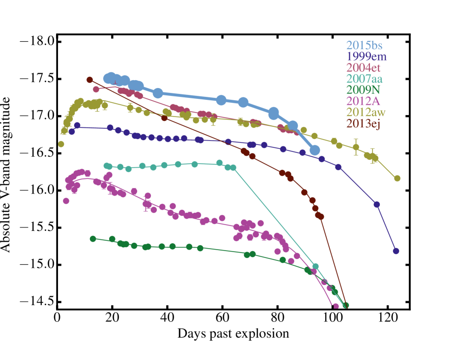
Figure 1: Absolute $V$-band light-curves of SN 2015bs together with a comparison sample from the literature. The light curve of SN 2015bs is shown in light blue. Errors on the photometry of SN 2015bs are the propagated errors from the photometric calibration (those for the comparison sample are taken from the literature). While SN 2015bs falls on the bright side of the distribution, overall it displays a normal light-curve morphology for a SN II. The decline rate during the ‘plateau’ phase appears typical of SNe II, as does the length of the optically thick phase duration.

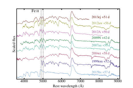
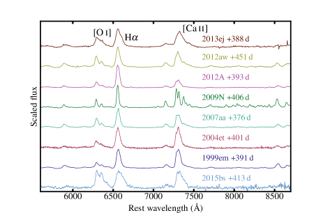
Figure 2: Comparison of optical-wavelength spectra of SN 2015bs with literature SNe II. a): photospheric phase spectra. While the Balmer lines appear similar between SN 2015bs and the comparison SNe, there is a clear lack of spectral features in the blue part of the spectrum. The position of the Fe ii 5018 Å absorption line is indicated, bracketed by dotted black vertical lines. This line has been used as a proxy for progenitor metallicity[22], and is significantly weaker in SN 2015bs. b): nebular phase spectra. The most prominent nebular lines are indicated on the spectrum of SN 2013ej: [O i] 6300,6364 Å; H$\alpha$; and [Ca ii] 7291,7323 Å. While the comparison SNe II all look quite similar – apart from small changes in the width of emission lines – SN 2015bs is clearly distinct. The relative strength of oxygen is much higher, and in particular H$\alpha$ is broader.

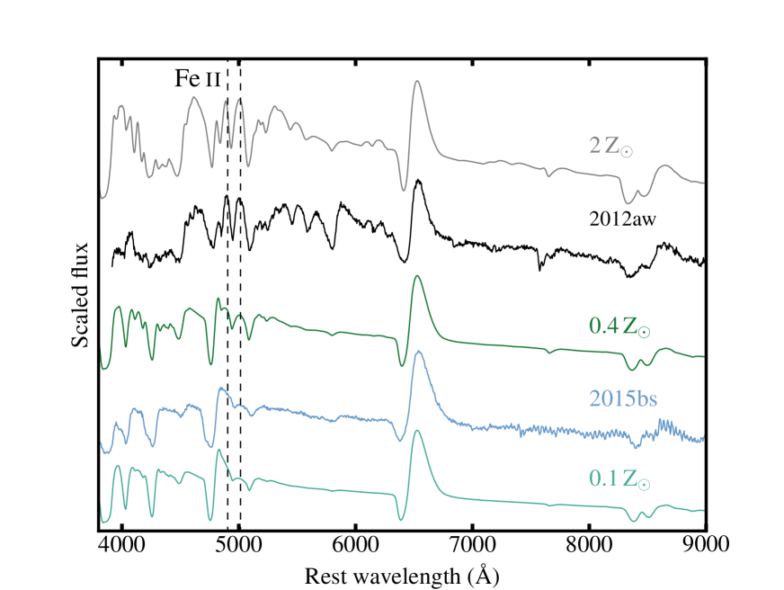
Figure 3: Comparison of the 57 d spectrum of SN 2015bs with 0.1${\rm\ Z}_{\odot}$ and 0.4${\rm\ Z}_{\odot}$ models at +50 d[3]. We also present an example SN II from our comparison sample (SN 2012aw) which shows much more prominent metal lines, more consistent with the 2${\rm\ Z}_{\odot}$ model. It is clear that the 0.1${\rm\ Z}_{\odot}$ model best matches the spectrum of SN 2015bs (observe the regions bluer than 5000 Å, and specifically the strength of the Fe ii 5018 Å line, which is bracketed by dashed lines), providing strong evidence for the low-metallicity nature of SN 2015bs.

Methods

1. CSS140925:223344-062208, aka SN 2015bs
SN 2015bs was discovered on the 25th of September 2014 by the Catalina Sky Survey (CSS) telescope of the overall CRTS project. In Supplementary Fig. 1 the position of the SN is indicated on a collapsed image produced from our integral field spectroscopy obtained using the Multi Unit Spectroscopic Explorer (MUSE[1]) at the Very Large Telescope, VLT. While no explosion-epoch constraining non-detections exist from the CSS, a non-detection from the Mount Lemmon facility (part of CRTS) on the 15th of September 2014 (limiting magnitude of 21.73) constrains the date of explosion to be the 20th of September 2014 $\pm$5 days, or Julian Date (JD) 2456920.5 $\pm$5 days. The transient was also detected much later by Pan-STARRS1 as PS15dsr on the 27th June 2015, at $w_{\rm ps}$ = 21.3 mag. A spectrum was obtained with the ESO Faint Object Spectrograph and Camera (v.2) (EFOSC2[2]) mounted on the New Technology Telescope (NTT) on September the 29th 2014[3] (see Supplementary Fig. 2), revealing a type II spectral morphology. Matching of the classification spectrum with a library of SN spectral templates using SNID[4] gives good results with SN 2004et at 2 days before maximum light, which translates to 14 days post explosion (+14 d), leading to an explosion epoch of the 15th of September, i.e. the same date as the last non-detection. The reason for the earlier explosion epoch from the spectral matching can be explained by the low progenitor metallicity of SN 2015bs, meaning that spectral line and colour evolution is slower than usually observed in SNe II (because of reduced blanketing by metal lines[5]). Nevertheless, the spectral matching gives an explosion epoch that is overall consistent with that from the non-detection.
We identify narrow H$\alpha$ emission from a galaxy (indicated in Supplementary Fig. 1) offset 3.4^′′ from SN 2015bs (the characterisation of which is presented below). The observed wavelength of this emission (the only emission line observed for this galaxy) gives a redshift for that object of 0.027. This redshift is consistent with that of the SN H$\alpha$ emission as seen in the nebular spectrum, and the value inferred from spectral matching above. We adopt this redshift for SN 2015bs, which corresponds to a distance modulus of 35.4 mag (assuming $H_{0}$ of 73 km s^-1 Mpc^-1). At this redshift, the angular separation between the peak flux of our identified host and SN 2015bs translates to 2 kpc.
Line of sight extinction from dust contained within the Milky Way is taken from the recalibrated dust maps of [6], assuming a Fitzpatrick extinction law[7]. No sign of narrow sodium absorption within the spectra of SN 2015bs is detected – the presence of which would indicate a higher level of host galaxy extinction – and as shown below in Section 3 and Supplementary Fig. 3, SN 2015bs does not show particularly red colours. Therefore we assume that SN 2015bs is affected by negligible internal host galaxy extinction.

2. Data reduction and calibration
$BVri$ photometry was obtained through the Carnegie Supernova Project-II (CSP-II[8]) from around maximum light to just after the end of the plateau, using the Swope telescope (+ e2V CCD) at the Las Campanas Observatory. Images were reduced in a standard manner. Observations of standard star fields were carried out on photometric nights when SN 2015bs was observed allowing the calibration of local standard sequences in $BV$[9] and $ri$[10]. Photometry of SN 2015bs was then calibrated against these local sequences, and is published in the natural system of the Swope telescope. Photometry of local sequence stars is presented in Supplementary Table 1 (on the standard system), while that of SN 2015bs is listed in Supplementary Table 2 (on the natural system). No attempts were made to subtract the underlying host galaxy flux, given that the host is not detected in deep images taken around a year post explosion. The $BVri$ light-curves for SN 2015bs are displayed in Supplementary Fig. 4.
The Pan-STARRS Survey for Transients observed the field of SN 2015bs during the tail phase, some 280 days after discovery during its normal survey mode. The transient was recovered over a period of 77 days with the internal name PS15dsr. The data were taken with the broad $w_{\rm ps}$ band which is a composite of $g_{\rm ps}r_{\rm ps}i_{\rm ps}$, as described in [11]. Difference imaging with respect to a reference frame was carried out, with point-spread-function photometry produced automatically as described in [12] and [13]. The detections from Pan-STARRS difference images are associated and merged into objects in a database of transients[14] and the photometry is reported in Supplementary Table 3 (AB magnitudes in the system described by [15])
Four photospheric-phase optical spectra were obtained for SN 2015bs using the NTT (+ EFOSC2) at La Silla, through the PESSTO collaboration, and using the Las Cumbres Observatory (LCO[16]) FLOYDS spectrograph. Spectra were obtained at +9 (the classification spectrum discussed above), +23, +57 and +80 d. The photospheric-phase spectral sequence is presented in Supplementary Fig. 2. EFOSC2 spectra were reduced and calibrated in a standard manner using a custom built pipeline for the PESSTO project[23], while the FLOYDS spectrum was reduced as in [17].
The position and surrounding sky of SN 2015bs were observed using MUSE at +406 and +421 d. MUSE is a 1^′$\times$1^′ field of view (FOV) integral field spectrograph, allowing us to simultaneously observe the SN and search for its host galaxy. These data were reduced using the MUSE pipeline[18], with subsequent combination of the two observations. The extracted 1 dimensional spectrum of SN 2015bs is shown in Fig. 2 of the main article. The MUSE data cube was analysed using QFitsView[19].
Throughout our analysis we compare the properties of SN 2015bs with a sample of SNe II from the literature. Given that our conclusions stem from analysis of nebular-epoch optical spectroscopy, our comparison sample was defined as any SN II with a nebular spectrum (with a cut off date of December 2015) within $\pm$50 days of that obtained for SN 2015bs, with respect to the explosion. Seven such SNe were found which are listed in Supplementary Table 4.

3. Nebular line analysis of SN 2015bs with respect to a SN II comparison sample
Nebular spectra of SNe II are dominated by H$\alpha$, [O i] 6300,6364 Å, and [Ca ii] 7291,7323 Å, and our analysis is restricted to the measurement of these line profiles. We measure FWHM velocities, and in the case of [O i] and [Ca ii] their absolute fluxes. Velocities are extracted by fitting Gaussians to each line and measuring their FWHM. In the case of [Ca ii], often more than two Gaussians are needed to provide a good fit. This is to be expected, as the [Ca ii] lines can be blended with e.g. [Ni ii] 7378 Å, [Fe ii] 7388 Å, and [Ni ii] 7412 Å. In addition, for SN 2015bs and SN 2013ej, more than two components are needed for [O i], and more than one component for H$\alpha$ (arguing against unusually strong [Ni ii] 7378 Å, [Fe ii] 7388 Å, and [Ni ii] 7412 Å in these SNe II, given that the ‘red-excess’ is not unique to [Ca ii]). In the case of SN 2013ej, it has been suggested that the nebular lines are best modelled assuming blue- and red-shifted components of [O i], H$\alpha$, and [Ca ii][20]. Additional components on the red side of [O i] and H$\alpha$ were also observed for SN 2014G[21], and were argued to be due to circumstellar interaction. SN 2015bs displays [O i], H$\alpha$ and [Ca ii] emission peaks blue-shifted by around 1000 kms^-1. Excess flux is also observed as a red shoulder in emission lines (see Supplementary Figs 8 and 11). Such profiles could suggest significant dust extinction in SN 2015bs. Alternatively, ejecta asymmetries may explain the observed line profiles. Given that we also observe both blue-shifted emission and a red-shoulder excess for [Ca ii] 7291,7323 Å suggests that a strong ejecta asymmetry is most likely, as this line predominantly forms outside the metal core where any dust would reside.
If a better fit to the line profiles is attained using additional Gaussian components then these are added, and the [O i], H$\alpha$, and [Ca ii] velocities are taken from the largest fitted Gaussian. To estimate line fluxes we simply integrate the total emission under the [O i] and [Ca ii] line profiles. This is achieved over a constant wavelength range for all SNe, meaning that we include any ‘extra’ emission observed in the case of [O i], and that from [Ni ii] 7378 Å, [Fe ii] 7388 Å, and [Ni ii] 7412 Å in the case of [Ca ii]. This approach is preferred, given the uncertain nature of fitting to multiple unresolved lines, and it also allows for a consistent comparison between all SNe. In this case the values presented here are not immediately comparable to those published elsewhere[31].
Histograms of FWHM velocities of [O i], H$\alpha$, and [Ca ii] are shown in Supplementary Fig. 7. With respect to the comparison sample, SN 2015bs shows nebular-phase velocities for [O i] and [Ca ii] towards the centre of the distributions. However, SN 2015bs clearly displays the highest H$\alpha$ velocity (Supplementary Figs 8 and 9). Larger nebular-phase velocities are expected in the case of SNe II with higher helium core masses[4]. As discussed in the main article, we make direct comparison of the nebular-phase H$\alpha$ velocity measured for SN 2015bs with those from the hydrodynamic models of [4], constraining the progenitor mass of SN 2015bs to be as high as 25${\rm\ M}_{\odot}$ (further details below). The ‘normal’ line velocities for [O i] are to be expected for a larger progenitor mass where a higher percentage of the flux is expected to arise from the core (i.e. a reduced [O i] flux from faster moving outer envelope).
The nebular-line widths are measured directly from the nebular spectrum. However, in order to extract a photospheric-phase velocity – and directly compare observed velocities to model values from [4] – we use two SNe II from our comparison sample to aid us. This is because the spectral lines usually used for estimating the photospheric velocity, such as Fe ii 5169 Å are weak in the photospheric-phase spectra of SN 2015bs, making their use unreliable. Therefore, we calibrate the velocity difference between H$\beta$ and Fe ii 5169 Å for SN 2004et and SN 2013ej (given their similar H$\beta$ and H$\alpha$ velocities to SN 2015bs), and apply this difference to the H$\beta$ velocity for SN 2015bs, obtaining a +50 d photospheric velocity of 5359 $\pm$ 392 kms^-1. Using this, together with the nebular-epoch HWHM velocity of H$\alpha$ of 2127 $\pm$ 308 kms^-1, thus constrains (through comparison to hydrodynamic models) the initial progenitor mass of SN 2015bs to be between 20 and 25${\rm\ M}_{\odot}$.
In the main article the flux of [O i] with respect to the flux of that across the full wavelength range of the MUSE spectrum was presented for SN 2015bs as compared to the same measurement for our comparison sample and SN 1987A. This showed that SN 2015bs indeed displays stronger [O i] with respect to the available energy (⁵⁶Co decay). Previously, the luminosity of [O i] as a percentage of the total ⁵⁶Co power at the epoch of observations has been used as a proxy for progenitor mass through model comparisons[13]. Here we also analyse SN 2015bs in this context. To estimate a ⁵⁶Ni mass for SN 2015bs we proceed with three different methods. Firstly, we extract a synthetic $V$-band magnitude from the nebular MUSE spectrum obtained at around +400 d, which we estimate to be 24.11$\pm$0.66 mag. This magnitude is then converted into a bolometric luminosity, and a ⁵⁶Ni mass of 0.048${}^{+0.041}_{-0.022}$${\rm\ M}_{\odot}$ is derived assuming full trapping of the radioactive emission by the SN ejecta[22]. Secondly, we integrate the total flux within the MUSE spectrum (4800 to 9300 Å), together with the ‘MUSE flux’ of a spectrum of SN 1987A close in time to that of SN 2015bs[23]. Converting these fluxes to luminosities we then obtain the ratio of SN 2015bs MUSE luminosity to that of SN 1987A, and using a ⁵⁶Ni mass of 0.075 for SN 1987A[24], we arrive at a value for SN 2015bs of 0.042${}^{+0.006}_{-0.007}$${\rm\ M}_{\odot}$. Finally, a ⁵⁶Ni mass is estimated using late-time $w_{\rm ps}$-band photometry. We first fit a straight line to the $w_{\rm ps}$-band photometry, confirming a decline rate consistent with that expected by the decay of ⁵⁶Co. We then extrapolate this (by 50 days) to the epoch at which there is a spectrum available for SN 1987A. A ⁵⁶Ni mass of 0.057${}^{+0.003}_{-0.003}$${\rm\ M}_{\odot}$ for SN 2015bs is then obtained by scaling the brightness of the SN 2015bs photometry to that of SN 1987A. Taking an average of these three values we obtain a ⁵⁶Ni mass of 0.049$\pm$0.008${\rm\ M}_{\odot}$.
Using the derived ⁵⁶Ni mass for SN 2015bs the luminosity of [O i] is estimated as a percentage of the ⁵⁶Co power to be 5.3%. This is much higher than any previous SN II (see Fig. 24 of reference [25], where the previous highest value was less than 4%), and when compared to model predictions suggests a ZAMS mass of $\geq$17-18${\rm\ M}_{\odot}$ (estimated from figure 24 of [25]), consistent with the mass estimates from [O i] fluxes as compared to models in the main article using the [O i] flux compared to the total MUSE flux, and comparison to such constraints for SN 1987A.
The overall results from this nebular analysis are shown in Supplementary Fig. 10. Here two ratios are plotted vs. each other. On the x-axis the ratio of the nebular to photospheric-phase H$\alpha$ velocity is shown. This normalises the outer core velocity to the explosion energy[4]. On the y-axis we show the ratio of the integrated flux of [O i] to that of [Ca ii]. SN 2015bs falls on the extreme of the distribution of each axis, confirming its uniqueness. Based on model predictions[4, 5], the simplest explanation is that SN 2015bs was the explosion of a massive, 17-25${\rm\ M}_{\odot}$ progenitor star, i.e. the most massive progenitor star yet inferred for a SN II.

4. Host galaxy identification and characterisation
There is a faint galaxy 12.7^′′ away from the explosion position of SN 2015bs (see Supplementary Fig. 1), however this galaxy does not have a published redshift and appears as a candidate SDSS galaxy. The initial redshift of 0.021 was taken from the SN spectral matching (see above). This implied an absolute $r$-band magnitude of –13.6 mag for the galaxy: already one of the dimmest hosts for a SN II. However, in our MUSE observations [O ii] 3727 Å and H$\beta$ emission are identified for this galaxy at a redshift of 0.90, inconsistent with our initial redshift estimate and therefore this galaxy was discarded as the possible host. The host of SN 2015bs was identified as a very faint galaxy (see Supplementary Fig. 1) that has narrow H$\alpha$ emission at a wavelength consistent with SN 2015bs. Only H$\alpha$ is visible in the spectrum, so we are unable to constrain the metallicity using emission line diagnostics. This provides a compelling argument for the use of SN II as independent metallicity indicators. A synthetic $r$-band magnitude was extracted from the host galaxy spectrum and estimated to be 23.3$\pm$0.2 mag. Correcting this for Milky Way extinction, and the distance modulus, we obtain an absolute $r$-band magnitude of –12.2, making the host of SN 2015bs the dimmest host for a SN II in the literature. Aware of the caveats of converting this to a metallicity, this implies a chemical abundance of 0.04$\pm$0.05 ${\rm\ Z}_{\odot}$[19], making SN 2015bs the lowest host metallicity SN II yet studied. The metallicity error is that of the dispersion on the relation between absolute magnitude and metallicity from [19].

Data Availability Statement
The data that support the plots within this paper and other findings of this study are available from the corresponding author upon reasonable request. In addition, the PESSTO spectra are available through the PESSTO Spectroscopic Data release 3 (SSDR3), for more information see the PESSTO website (www.pessto.org), all spectra will also be made available on WISeREP: www.weizmann.ac.il/astrophysics/wiserep/, and photometric measurements are listed in the SI.

References

Supplementary Information

1. Characterisation of SN 2015bs
To characterise SN 2015bs we use a number of parameters that have been defined to study the $V$-band light-curves of type II supernovae (SNe II), including magnitudes at various epochs, decline rates at different epochs, and duration of different phases[1]. All measured parameters are listed in Supplementary Table 5. Also listed in the table are the mean values of these same parameters as measured for a large sample of $>$ 100 SNe II[1]. SN 2015bs is a bright SN II, characterised by a relatively flat light-curve, a relatively short plateau duration (Pd), and a relatively high ⁵⁶Ni mass. (At nebular times, and in the absence of other sources like interaction with circumstellar material or radiation from a compact remnant, the SN luminosity is powered exclusively by the decay of ⁵⁶Co. The decay chain is ⁵⁶Ni to ⁵⁶Co to ⁵⁶Fe, with a half-life for ⁵⁶Ni and ⁵⁶Co of 6.0749 d and 77.233 d.). However, all of the measured parameters fall within the distribution of literature SNe II. This is also seen in the absolute $V$-band light curves plotted in Fig. 1 of the main article.
In Supplementary Fig. 4 we show the $B-V$ and $V-i$ colour curves of SN 2015bs and the comparison sample. To produce these curves, magnitudes are corrected for both MW and internal host galaxy extinction (with the latter taken from the references in Supplementary Table 5). In $B-V$, SN 2015bs falls on the blue side of the distribution, however, again it does not seem peculiar in any way. In $V-i$ SN 2015bs falls within the central part of the distribution.
The final comparison we make is through measurements of ejecta expansion velocities. In Supplementary Fig. 5 we plot the time evolution of H$\alpha$ (from the Full Width Half Maximum, FWHM, of the line profile) and H$\beta$ (from the minimum of the absorption trough) spectral velocities for SN 2015bs together with those for the SN II comparison sample. SN 2015bs displays some of the highest velocities, however their values and time evolution fall within the observed range of SNe II. One may speculate that the lack of strong metal lines may be an effect of high expansion velocities blending relatively weak metal lines into the continuum. However, even in high energy photospheric models such lines are clearly visible[3], and such a scenario does not seem to be at play in the case of SN 2015bs.
After the characterisation and comparison provided above, we conclude that SN 2015bs is a relatively normal SN II. This event does not appear to be peculiar during the photospheric phase (except for the strength of metal lines, as outlined below). Following this, the progenitor of SN 2015bs was most likely a red supergiant (RSG) star, consistent with literature constraints on other SNe II.

1.1 The lack of metal lines in the +57 d spectrum
The photospheric-phase spectra of SN 2015bs, as presented in Supplementary Fig. 2, show a clear lack of metal lines. This is particularly apparent blue ward of H$\alpha$  and in the ‘cleanness’ of the full Balmer series. To our knowledge, such a spectrum has not been observed previously. In Supplementary Fig. 6 we present a comparison of the +57 d SN 2015bs spectrum with those from [26], with the latter SNe II showing the lowest Fe ii 5018 Å pEWs within their sample. Compared to the SNe II from [26], SN 2015bs displays a remarkable similarity to the 0.1${\rm\ Z}_{\odot}$ model spectrum. The comparison SNe II in Supplementary Fig. 6 indeed show relatively weak lines, but none display such a similarity to the 0.1${\rm\ Z}_{\odot}$ model as SN 2015bs, and additionally these comparison SNe II display properties marking them out as abnormal events, while SN 2015bs appears as a standard SN II with its metal lines absent.
Metal line strength in photospheric-phase spectra of SNe II was first predicted[3], and then shown observationally[22], to be dependent on progenitor metallicity. The appearance of the SN 2015bs +57 d spectrum suggests a low-metallicity progenitor. Fig. 3 in the main article presented a comparison between the SN 2015bs +57 d spectrum and 0.1${\rm\ Z}_{\odot}$ and 0.4${\rm\ Z}_{\odot}$ model spectra, together with an example of a probable higher progenitor metallicity observed SN II in comparison to a 2${\rm\ Z}_{\odot}$ model. The match between SN 2015bs and the 0.1${\rm\ Z}_{\odot}$ model is remarkable, given that the models were not tailored to fit any SN in particular. Measuring the Fe ii 5018 Å pEW in the +57 d spectrum we obtain 4.25$\pm$0.54 Å. Comparing this to a large sample of such measurements[1], SN 2015bs has the 2nd lowest pEW with respect to all SNe II at +50 d. The lowest, SN 2005dn has an pEW of 4.1$\pm$0.7 Å. The estimated oxygen abundance for the host H ii region of SN 2005dn is $<$8.15 dex (on the N2 scale[2]). SN 2005dn is a somewhat fast decliner, with an $s_{2}$ value of 1.55 mag 100 days^-1. Another key difference between SN 2005dn and SN 2015bs is that while SN 2005dn has a low Fe ii 5018 Å pEW, it displays many additional stronger lines between H$\alpha$ and Fe ii 5018 Å pEW that are almost non-existent in SN 2015bs (see Supplementary Fig. 2). There are two other SNe with pEWs less than 7Å. These are SN 2006Y and SN 2008gr. Both of these SNe are fast decliners and would not be considered ‘plateau’ SNe II. SN 2008gr, in a similar fashion to SN 2005dn discussed above, presents numerous other metal lines blue ward of H$\alpha$. In the case of SN 2006Y, this is a very non-standard SN II and hence any comparison to our ‘normal’ SN II 2015bs is not particularly useful. The spectra of low-Fe ii 5018 Å pEW SNe II presented by [26] also display different properties as compared to the 0.1 ${\rm\ Z}_{\odot}$ model and SN 2015bs, as shown in Supplementary Fig. 6 (with the latter two being remarkably similar).
In conclusion, SN 2015bs displays the closest resemblance of any SN II in the literature to the low-metallicity 0.1 ${\rm\ Z}_{\odot}$ model, presenting an incredibly ‘clean’ spectrum between H$\alpha$ and Fe ii 5018 Å. Based solely on the photospheric-phase spectrum of SN 2015bs, this is the clearest candidate yet for a $\leq$0.1${\rm\ Z}_{\odot}$ progenitor SN II. (The SN II, LSQ13fn, was claimed to arise from a $\sim$ 0.1${\rm\ Z}_{\odot}$ progenitor[3]. However, LSQ13fn was a non-standard SN II – it was particularly blue, it does not follow the magnitude–velocity relation – while still displaying significant differences with respect to the 0.1${\rm\ Z}_{\odot}$ model.) This conclusion is confirmed by our host galaxy analysis, and further supports the use of SN II spectra as metallicity indicators, especially in the case when no host galaxy constraints are available.

2. Progenitor mass constraints from nebular-line analysis
Most of our conclusions are grounded on models that predict a strong relationship between helium core mass (the property being probed by nebular-phase spectroscopy), and Zero Age Main Sequence (ZAMS) mass[28]. However, stellar rotation is known to affect massive star evolution[4]. In particular, models with higher initial rotation rates tend to produce more massive helium cores[10]. While observationally such rotational effects are unconstrained for SNe II, in the case of SN 2015bs the progenitor may be affected by different degrees of rotation, hence affecting the properties of the resulting SN. There is some evidence that lower-metallicity massive stars have higher rotational velocities[5] (but with large dispersion and many low-rotation stars being also found within low-metallicity environments). It is therefore a possibility that the high core mass estimated for SN 2015bs is a product of a lower ZAMS progenitor than usual, due to a higher initial rotation. However, while we cannot rule out this possibility, currently this is somewhat speculative. An additional uncertainty lies with the treatment of convection in 1-D (spherically symmetric) stellar evolution models[29], which may lead to uncertainty in the exact mapping of helium-core mass back to ZAMS. Stellar evolution models that include rotation and/or a 3-D treatment of convection etc are lacking, and, therefore, spectral models based on such progenitors are also lacking. For nebular models that do exist[4, 12], SN 2015bs is consistent with a relatively massive progenitor. In massive stars the helium core is formed during the hydrogen-burning phase[9], which is largely over when the star becomes a RSG. The bulk of the mass loss by a 15-30${\rm\ M}_{\odot}$ star, during the RSG phase and thus after the helium core is formed[9]. Therefore uncertainties in RSG mass-loss rates (and their dependence on metallicity and rotation) have little impact on our helium core mass constraints for SN 2015bs. The effect of progenitor metallicity on helium core mass is indeed found to be negligible up to an initial mass of about 28${\rm\ M}_{\odot}$[9], and this is also illustrated by simulations[3]. 15${\rm\ M}_{\odot}$ stars of 0.002, 0.008, 0.02 and 0.008 metallicity evolved using standard stellar evolution prescriptions (in particular the dependence of mass loss on metallicity) and exploded to produce transients with light-curves and spectra consistent with standard SNe II produced helium core masses that range from 4.15${\rm\ M}_{\odot}$ for the lowest to 3.77${\rm\ M}_{\odot}$ for the highest metallicity cases[3]. Therefore, only a 10% change in helium core mass is observed from a change of a factor of 20 in metallicity. This change is too small to explain the unique properties of the nebular-phase properties of SN 2015bs. While future nebular-phase spectral modelling using a large range of progenitor properties will certainly be useful for this type of study, comparison with current models suggest a relatively large ZAMS for SN 2015bs.

3. Comparison to Jerkstrand models and SN 1987A
Above we analysed and discussed specific line measurements of SN 2015bs in its nebular-phase spectrum and their implications for the helium core-mass and progenitor mass. In this sub-section we directly compare our nebular spectrum to a) model nebular spectra, and b) a nebular spectrum of the intensely studied SN II 1987A.
Supplementary Fig. 11 shows a comparison between the 15 and 25${\rm\ M}_{\odot}$ ZAMS Jerkstrand models[12] at +400 d, with our nebular spectrum of SN 2015bs. The observed and model spectra display reasonable agreement overall. The strength of the [Ca ii] 7291,7323 Å lines are very similar, while the H$\alpha$ flux is considerably higher in the 15${\rm\ M}_{\odot}$ model as compared to SN 2015bs. SN 2015bs falls between the 15 and 25${\rm\ M}_{\odot}$ models with respect to the relative strength of [O i]. While one may therefore conclude that this implies a $\sim$20${\rm\ M}_{\odot}$ ZAMS mass for SN 2015bs, within the models the strength of [O i] does not increase linearly between 15 and 25${\rm\ M}_{\odot}$[12] (unfortunately there is no 19${\rm\ M}_{\odot}$ model at +400 d). Compared to this set of models, SN 2015bs is therefore consistent with a progenitor ZAMS mass of 17-18${\rm\ M}_{\odot}$, although as above we note that model line fluxes start to saturate above 19${\rm\ M}_{\odot}$, meaning that models in the 20-30${\rm\ M}_{\odot}$ range are only 20-30 brighter than the measured luminosity, and cannot be ruled out considering uncertainties in the modelling.
SN 1987A remains the closest observed SN to Earth to explode within the last $\sim$400 years. While the light-curve displayed a rare long rise to maximum, and therefore the event itself is not directly comparable to the ‘normal’ SNe II discussed here, given the wealth of information we have on this event and its progenitor, a direct comparison between SN 1987A and SN 2015bs is warranted. Many progenitor models have been produced for SN 1987A[6], however we still lack an adequate model that explains all properties of the observed progenitor, the SN light-curve and its spectral morphology[6]. Models in best agreement with observations of SN 1987A and its progenitor fall in the range 15 to 20${\rm\ M}_{\odot}$[6, 7, 8]. With these constraints in mind a direct comparison of our nebular spectrum of SN 2015bs with that of SN 1987A at a similar epoch is presented in Supplementary Fig. 12. Overall the spectra appear quite similar, however the relative strength of the nebular lines is somewhat different. SN 2015bs displays stronger [O i] but weaker [Ca ii] and H$\alpha$ than SN 1987A. Taking the strength of the [O i] as a direct He-core and therefore ZAMS progenitor mass indicator, this suggests that SN 2015bs arose from a higher mass progenitor than SN 1987A. Given the relatively large progenitor masses (as compared to the current population of direct progenitor detections for ‘normal’ SNe II) discussed for SN 1987A, this comparison brings further support to our conclusion that SN 2015bs arose from the highest progenitor yet observed for a SN II, with an overall range of 17-25${\rm\ M}_{\odot}$. Indeed, the direct comparison here with SN 1987A would suggest masses in the higher end of this range.

4. The red supergiant problem
Our interest in the discovery of a high-mass progenitor for a SN II is motivated by the previous apparent non-detection of high mass progenitors associated with SN II explosions. This ‘red supergiant problem’ refers to the lack of SN II progenitors with masses higher than $\sim$18${\rm\ M}_{\odot}$[1]. This is a problem because RSGs of up to 30${\rm\ M}_{\odot}$ are observed[2] and at least some are expected to explode as SNe II, as they probably lose insufficient mass during their late phases to explode as SNe of types IIb, Ib or Ic (‘stripped-envelope SNe’, SE-SNe). However, model predictions for the mass-limit for producing SNe II or SE-SNe are heavily dependent on the mass-loss rates employed and the inclusion and degree of rotation assumed[10, 9, 11, 10], and it has been claimed that the RSG problem simply does not exist[11] when using sufficiently high mass-loss rates[11]. If one assumes significant rotation and/or high mass-loss rates, then stars initially more massive than $\sim$18${\rm\ M}_{\odot}$ may evolve to explode as non-SN II types. RSG mass-loss rates are hugely uncertain (see e.g. [12] for a review), with significant differences between different recipes[11, 9]. High mass-loss rate prescriptions[11], have been used in stellar evolution models to demonstrate that $<$20${\rm\ M}_{\odot}$ stars can explode as e.g. SNe IIb[13]. However, a consensus to apply such large mass-loss rates to all RSGs and to the overall evolution of these stars (in place of specific phases of possibly enhanced mass-loss) is still lacking, and there is no general agreement on which mass-loss rates one should employ. While it is possible to produce SE-SNe for $\sim$20${\rm\ M}_{\odot}$ progenitors when using the highest RSG mass-loss rates, there are many RSGs that are observed to lose mass at a much lower rate and hence may not lose enough mass to avoid exploding as a type II SN (see e.g. figure 1 in [14] for a comparison of different mass-loss estimates for RSGs).
This red supergiant problem also emerges from nebular spectroscopic studies[12], together with the analysis of parent stellar populations of SN remnants[15]. We have also not detected any clear cases of SNe types II, IIb, or Ib with progenitors of 20-30${\rm\ M}_{\odot}$. If $>$18${\rm\ M}_{\odot}$ progenitors explode as non-SNe II then we should have detected their progenitors. Both constraints on SNe IIb and Ib ejecta masses[16, 17, 19, 18], and their relative rates[20] suggest that the majority of these explosions do not arise from $>$20${\rm\ M}_{\odot}$ explosions, but rather lower-mass progenitors that lose their mass through binary interaction. It has been argued[15] that progenitors could be affected by unaccounted for circumstellar dust, therefore lowering their progenitor luminosities and estimated masses. However, in the particular case of SN 2012aw the correct treatment of the dust revealed a relatively low progenitor mass[21] (after initially higher estimates). If unaccounted for circumstellar dust is affecting derived progenitor luminosities, then an interesting possibility is that this preferentially affects the higher-metallicity cases where it is assumed that dust production is easier. This could then be consistent with our conclusion of a low-metallicity–high-mass progenitor for SN 2015bs.
An overall relatively low-mass progenitor population for SNe II is also consistent with the low x-ray luminosities measured for SNe II[22] (see [1] for detailed discussion of all these possibilities and why – in their view – they are unlikely). Most recently, it has been claimed[16] that the lack of high-mass RSGs exploding as SNe II is due to the incorrect use of fixed bolometric corrections for estimating progenitor luminosities. [16] argue that bolometric corrections for RSGs change as stars come closer to core-collapse and that when this is taken into account the observed upper limit of progenitors comes into line with observed RSG masses in the local Universe.
The above discussion highlights the current problems in trying to understand the RSG problem, with explanations ranging from: ‘there is no problem, $>$20${\rm\ M}_{\odot}$ stars don’t explode as RSGs at solar metallicity because of mass-loss’, or ‘there is no problem as bolometric corrections are incorrectly applied to obtain progenitor luminosities’ to the original claim that there are RSGs that should explode as SNe II but don’t, which together with the lack of detected SE-SNe arising from $>$20${\rm\ M}_{\odot}$ progenitors leads to a real problem of a lack of massive star explosions.
One possibility – whether the RSG problem exists or not – is that the majority of massive progenitors do not explode as successful SNe, but instead collapse to black holes with weak or no accompanying outburst[7]. Several independent studies have discussed the ‘compactness’ parameter (basically the core radius within which a certain mass is confined) as determining whether a successful explosion will occur[32, 23, 24]. These studies suggest that it is indeed more difficult to explode more massive stars, with only small regions of the $>$20${\rm\ M}_{\odot}$ progenitor parameter space producing successful explosions, i.e. the ‘islands of explodability’ (see [33] for a successful explosions of a 27${\rm\ M}_{\odot}$ star). The case for failed explosions above 18-20${\rm\ M}_{\odot}$ is also supported by the compact remnant mass function that is found to be bimodal (between neutron stars and black holes). A continuous function would be expected for a continuous range of successful explosions[25], however the observed bimodal mass function is a direct prediction of failed explosions[17]. Finally, the discovery of the disappearance of a $\sim$25${\rm\ M}_{\odot}$ RSG has provided direct evidence for a failed SN[18] (see also [26]). This gives one specific example of a massive RSG that died with a massive and extended hydrogen-rich envelope but did not explode as a luminous transient.
It is in the above context that our conclusions of a massive 17-25${\rm\ M}_{\odot}$ ZAMS mass progenitor for SN 2015bs are placed. Our detection of a massive RSG exploding as a SN II, together with the failed explosion of a similarly massive star[18], suggest that predicted ‘islands of explodability’ may indeed exist. At the same time, the low-metallicity nature of SN 2015bs possibly suggests that a prerequisite for SN II explosions from progenitors above 18-20${\rm\ M}_{\odot}$ may be low metallicity, with higher metallicity progenitors exploding as SE-SNe. However, the detection of a disappearing $\sim$25${\rm\ M}_{\odot}$ RSG at solar metallicity suggests that this cannot be the case for all RSGs. A high-mass SN IIb or SN Ib progenitor at solar-metallicity is required to support this latter scenario.

References

List of suppfigures 1 MUSE image of SN 2015bs and its surroundings. This is formed by collapsing the data cube across the full wavelength range of the observation. SN 2015bs together with its host and the originally identified possible (SDSS) host are indicated on the image. The hatched line pattern observed is due to the edges of the individual IFUs within MUSE.

List of suppfigures 2 Photospheric phase spectral observations of SN 2015bs. The epochs post explosion are indicated on the plot.

List of suppfigures 3 $B-V$ (top) and $V-i$ (bottom) colour curves for SN 2015bs and our comparison sample.

List of suppfigures 4 $BVri$ light-curves of SN 2015bs. Photometric errors are the propagated errors from the photometric calibration.

List of suppfigures 5 H$\alpha$ FWHM (shown as circles), and H$\beta$ absorption minimum (presented as triangles) ejecta velocities for SN 2015bs and the SN II comparison sample. Velocity errors are the standard deviation of multiple spectral measurements with slight changes in the defined continuum level.

List of suppfigures 6 Comparison of the +57 d spectrum of SN 2015bs with that of the 0.1 ${\rm\ Z}_{\odot}$ model, together with a number of other SNe II displaying weak Fe ii 5018 Å lines in a region where line blanketing is strong at the recombination epoch in ${\rm\ Z}_{\odot}$ SNe II models and observations.

List of suppfigures 7 Histograms of the FWHM velocities of [O i] 6300,6364 Å, H$\alpha$ and [Ca ii] 7291,7323 Å. In each plot the position of SN 2015bs is indicated in blue, while the nebular SN II comparison sample is presented in maroon.

List of suppfigures 8 Nebular phase H$\alpha$ profile for SN 2015bs and all comparison SNe. Line profiles have been shifted in wavelength so that the peak of H$\alpha$ aligns for all SNe, and are normalised to the peak H$\alpha$ flux of SN 2015bs.

List of suppfigures 9 Ratio of the FWHM velocities of [O i] 6300,6364 Å to H$\alpha$ on the x-axis, compared with [Ca ii] 7291,7323 Å to H$\alpha$ on the y-axis. SN 2015bs is presented in blue, with the comparison sample in maroon. Ratio errors are propagated errors from the standard deviation of multiple spectral measurements of each feature with slight changes in the defined continuum level each time.

List of suppfigures 10 Ratio of the SN II integrated nebular [O i] 6300,6364 Å to [Ca ii] 7291,7323 Å fluxes plotted against the SN II ratio of the H$\alpha$ FWHM velocity at nebular epochs with respect to the photospheric velocity +15 d. SN 2015bs is shown in blue, with the rest of the sample in maroon. It is clear that in the y-axis SN 2015bs is very much at the extremity of the distribution, while in the x-axis SN 2015bs displays the highest ratio of nebular to photospheric-phase ejecta velocities. Ratio errors are propagated errors from the standard deviation of multiple spectral measurements of each feature with slight changes in the defined continuum level each time. (See Section 3 of Methods for details of how these parameters were measured for each SN.)

List of suppfigures 11 Comparison of the nebular spectrum of SN 2015bs with model spectra at similar epochs. The model spectra are produced by progenitors of 15 and 25${\rm\ M}_{\odot}$ at solar metallicity[12]. The spectra are scaled to the total flux contained within the MUSE wavelength range of the SN 2015bs spectrum.

List of suppfigures 12 Comparison of the SN 2015bs nebular spectrum with that at a similar epoch of SN 1987A. The spectra are scaled to the overal flux contained within the MUSE wavelength range of the SN 2015bs spectrum. Note the relative strength of [O i] in SN 2015bs with respect to SN 1987A, suggesting a higher progenitor mass for the former. In addition, this plot clearly shows the asymmetric nature of the emission lines of SN 2015bs.

List of supptables 1 SN 2015bs local sequence photometry in the standard systems[9, 10]

Star	RA	Dec	$B$ (mag)	$V$ (mag)	$r$ (mag)	$i$ (mag)
1	22:33:23.62	$-$6:24:24.31	13.827 (0.003)	$\cdots$	$\cdots$	$\cdots$
2	22:33:23.20	$-$6:28:33.77	14.400 (0.009)	13.849 (0.013)	$\cdots$	$\cdots$
3	22:34:09.33	$-$6:15:45.02	17.382 (0.079)	16.569 (0.023)	16.211 (0.032)	15.940 (0.013)
4	22:33:44.86	$-$6:18:27.14	15.000 (0.015)	14.295 (0.003)	$\cdots$	$\cdots$
5	22:33:53.94	$-$6:22:53.67	15.049 (0.006)	14.424 (0.003)	14.204 (0.003)	$\cdots$
6	22:33:49.00	$-$6:16:09.63	15.280 (0.015)	14.529 (0.006)	14.230 (0.006)	$\cdots$
7	22:34:03.75	$-$6:21:08.24	15.812 (0.012)	14.898 (0.007)	14.458 (0.006)	14.158 (0.009)
8	22:33:55.22	$-$6:18:58.88	15.740 (0.010)	14.929 (0.009)	14.541 (0.012)	14.232 (0.021)
9	22:33:32.02	$-$6:18:42.94	15.920 (0.018)	15.190 (0.004)	14.901 (0.013)	14.645 (0.015)
10	22:33:26.33	$-$6:25:43.01	16.268 (0.043)	15.291 (0.018)	14.766 (0.015)	14.260 (0.010)
11	22:34:12.19	$-$6:19:20.36	16.173 (0.038)	15.481 (0.010)	15.212 (0.016)	15.001 (0.014)
12	22:33:59.20	$-$6:18:44.41	16.134 (0.011)	15.512 (0.010)	15.292 (0.009)	15.119 (0.014)
13	22:34:07.89	$-$6:20:13.86	16.046 (0.017)	15.535 (0.013)	$\cdots$	15.232 (0.017)
14	22:33:33.85	$-$6:29:09.08	16.624 (0.033)	15.782 (0.009)	15.381 (0.012)	15.070 (0.013)
15	22:33:22.22	$-$6:16:26.54	16.678 (0.047)	16.145 (0.032)	15.947 (0.019)	15.754 (0.014)
16	22:33:26.96	$-$6:23:44.69	17.077 (0.051)	16.217 (0.020)	15.838 (0.016)	15.524 (0.014)
17	22:34:03.21	$-$6:14:55.80	17.347 (0.063)	16.275 (0.013)	15.677 (0.023)	15.212 (0.012)
18	22:33:21.69	$-$6:27:28.13	$\cdots$	16.215 (0.014)	15.840 (0.021)	15.580 (0.022)
19	22:33:34.72	$-$6:25:11.91	17.368 (0.093)	16.430 (0.019)	15.931 (0.021)	15.567 (0.018)
20	22:34:13.70	$-$6:29:22.95	17.291 (0.017)	16.461 (0.019)	15.988 (0.023)	15.749 (0.010)
21	22:33:49.54	$-$6:17:59.55	17.165 (0.011)	16.471 (0.018)	16.175 (0.027)	15.967 (0.027)
22	22:34:06.06	$-$6:24:04.69	17.006 (0.060)	16.516 (0.033)	16.347 (0.024)	16.200 (0.024)
23	22:34:02.12	$-$6:24:44.69	17.331 (0.050)	16.551 (0.020)	16.223 (0.030)	15.914 (0.028)
24	22:33:40.60	$-$6:28:32.55	17.272 (0.066)	16.573 (0.004)	16.246 (0.007)	15.970 (0.035)

List of supptables 1 In the first column local sequence star number is given. In columns 2 and 3 the RA and Dec coordinates are listed for each star (J2000.0). In columns 4, 5, 6, and 7 magnitudes are listed for each star as observed in the $B-$, $V-$, $r-$ and $i-$band respectively. Magnitude errors are given in parenthesis. Photometric errors are the propagated errors from the photometric calibration.

List of supptables 2 SN 2015bs photometry in the natural system of the Swope telescope

JD	Epoch (days post explosion)	$B$ (mag)	$V$ (mag)	$r$ (mag)	$i$ (mag)
2456938.6	18	18.249 (0.034)	18.032 (0.029)	17.880 (0.025)	18.015 (0.027)
2456939.6	19	18.332 (0.032)	18.015 (0.023)	17.860 (0.019)	18.017 (0.022)
2456940.5	20	18.288 (0.019)	18.051 (0.019)	17.854 (0.017)	17.997 (0.018)
2456941.5	21	18.367 (0.015)	18.042 (0.013)	17.899 (0.014)	17.992 (0.017)
2456942.5	22	18.380 (0.010)	18.067 (0.012)	17.884 (0.011)	17.995 (0.013)
2456944.5	24	18.459 (0.014)	18.058 (0.016)	17.903 (0.014)	18.004 (0.017)
2456947.6	27	18.559 (0.011)	18.123 (0.013)	17.858 (0.078)	$\cdots$
2456948.5	28	18.575 (0.012)	18.123 (0.012)	17.932 (0.011)	18.042 (0.016)
2456949.5	29	18.602 (0.012)	18.133 (0.011)	17.918 (0.011)	18.036 (0.013)
2456956.5	36	18.796 (0.016)	18.229 (0.013)	17.965 (0.016)	18.068 (0.016)
2456979.5	59	19.141 (0.018)	18.323 (0.014)	18.018 (0.014)	18.070 (0.017)
2456987.5	67	19.209 (0.019)	18.352 (0.014)	18.031 (0.013)	18.064 (0.020)
2456998.5	78	19.342 (0.068)	18.519 (0.036)	18.110 (0.020)	18.130 (0.023)
2456998.5	78	19.575 (0.083)	18.484 (0.035)	18.163 (0.023)	18.100 (0.021)
2457005.5	85	19.687 (0.047)	18.667 (0.030)	18.272 (0.042)	18.256 (0.039)
2457013.5	92	20.173 (0.052)	18.996 (0.027)	18.558 (0.019)	18.430 (0.024)

List of supptables 2 In the first column the Julian Date of the observations is listed, followed by the epoch post explosion in column 2. The $B-$, $V-$, $r-$, and $i-$band photometry are then listed in columns 3, 4, 5, and 6 respectively. Magnitude errors are given in parenthesis. Photometric errors are the propagated errors from the photometric calibration.

List of supptables 3 SN 2015bs $w_{\rm ps}$-band photometry from Pan-STARRS

MJD	Epoch (days post explosion)	$w_{\rm ps}$ (mag)
57200.5	280	21.38 (0.08)
57200.5	280	21.46 (0.07)
57200.5	280	21.52 (0.10)
57200.6	280	21.40 (0.08)
57226.4	306	21.73 (0.19)
57243.4	323	21.88 (0.21)
57275.3	355	22.33 (0.20)
57277.3	357	22.31 (0.17)

List of supptables 3 In the first column the Modified Julian Date of the observations is listed, followed by the epoch post explosion in column 2. Photometry is listed in columns 3. Magnitude errors are given in parenthesis. Photometric errors are the propagated errors from the photometric calibration combined with those arising from the difference imaging.

List of supptables 4 SN II nebular comparison sample

SN	Photometry	Photospheric-phase spectroscopy	Nebular spectroscopy
1999em	Galbany et al. (2016)[27]	unpublished	Elmhamdi et al. (2003)[28]
2004et	Misra et al. (2007)[29]	Sahu et al. (2006)[30]	Maguire et al. (2010)[31]
2007aa	unpublished	unpublished	Maguire et al. (2012)[31]
2009N	Takats et al. (2014)[32]	Takats et al. (2014)[32]	Maguire et al. (2012)[31]
2012A	Tomasella et al. (2013)[33]	Tomasella et al. (2013)[33]	Tomasella et al. (2013)[33]
2012aw	Bose et al. (2013)[34]	Dall’Ora et al. (2014)[35]	Jerkstrand et al. (2014)[12]
2013ej	Bose et al. (2015)[36]	Yuan et al. (2016)[20]	Yuan et al. (2016)[20]

List of supptables 4 References for data from the comparison SN II sample that have nebular spectrscopy within $\pm$50 days of that of SN 2015bs. In the first column the SN name is listed. In columns 2, 3, and 4 we list the reference for the photometry, photospheric-phase spectroscopy, and nebular-phase spectroscopy respectively.

List of supptables 5 SN 2015bs measured parameters

	$M_{\rm max}$ (mag)	$M_{\rm end}$ (mag)	$s_{\rm 1}$ (mag 100d-1)	$s_{\rm 2}$ (mag 100d-1)	${\rm Pd}$ (days)	${\rm OPTd}$ (days)	${}^{56}{\rm Ni}$ (${\rm\ M}_{\odot}$)
SN 2015bs	–17.54$\pm$0.05	–17.19$\pm$0.05	1.17$\pm$0.10	0.33$\pm$0.04	39.5$\pm$4	78.5$\pm$5	0.048$\pm$0.008
Mean A14	–16.74$\pm$1.01	–16.03$\pm$0.81	2.65$\pm$1.50	1.27$\pm$0.93	48.4$\pm$12.6	83.7$\pm$16.7	0.032$\pm$0.021

List of supptables 5 Measured parameters for SN 2015bs in the first row, and mean values from a large sample[1] in the second row. In column 2 we list $M_{\rm max}$, the absolute $V$-band magnitude at maximum light. In column 3 $M_{\rm end}$ , the absolute $V$-band magnitude at the end of the plateau. $s_{\rm 1}$ is listed in column 4 and $s_{\rm 2}$ in column 5, corresponding to the initial decline rate from maximum, and the second shallower decline rate during the plateau respectively (both in the $V$ band). In column 6 we list ${\rm Pd}$, the plateau duration, which is defined from the inflection point between $s_{\rm 1}$ and $s_{\rm 2}$ until the end of the plateau. ${\rm OPTd}$, the optically thick phase duration, is listed in column 7 and is the time duration between explosion and the end of the plateau. Finally in column 8 we give the ${}^{56}{\rm Ni}$ mass. Errors on the mean values are the standard deviation of the each distribution. Errors on $M_{\rm max}$ and $M_{\rm end}$ for SN 2015bs come from the uncertainties on the SN photometry combined with the distance uncertainty, while errors on the decline-rate measurements $s_{\rm 1}$ and $s_{\rm 2}$ are the straight-line fit errors on each parameter. The error on ${\rm OPTd}$ is dominated by the error on the explosion epoch of SN 2015bs, and the error on ${\rm Pd}$ arises from a combination of the error on the $s_{\rm 1}$–$s_{\rm 2}$ transition epoch and the error on the definition of the end of the plateau. Finally, the error on the ${}^{56}{\rm Ni}$ mass is the standard deviation of the three independent measurements are outlined in the text.

References

- [1] Smartt, S. J. Observational Constraints on the Progenitors of Core-Collapse Supernovae: The Case for Missing High-Mass Stars. Pub. Astro. Soc. Aust. 32, 16-38 (2015)
- [2] Levesque, E. M. et al. The Effective Temperature Scale of Galactic Red Supergiants: Cool, but Not As Cool As We Thought. Astrophys. J. 628, 973-985 (2005).
- [3] Dessart, L. et al. Type II-Plateau supernova radiation: dependences on progenitor and explosion properties. Mon. Not. R. Astron. Soc. 433, 1745-1763 (2013)
- [4] Dessart, L. et al. Determining the main-sequence mass of Type II supernova progenitors. Mon. Not. R. Astron. Soc. 408, 827-840 (2010)
- [5] Jerkstrand, A. et al. The progenitor mass of the Type IIP supernova SN 2004et from late-time spectral modeling Astron. Astrophys. 546, 28-49 (2012)
- [6] Li, W. et al. Nearby supernova rates from the Lick Observatory Supernova Search - II. The observed luminosity functions and fractions of supernovae in a complete sample. Mon. Not. R. Astron. Soc. 412, 1441-1472 (2011)
- [7] Falk, S. W. & Arnett, W. D. Radiation Dynamics, Envelope Ejection, and Supernova Light Curves. Astrom. Astrophys. Suppl. S. 33, 515-562 (1977)
- [8] Smartt, S. J., et al. The death of massive stars - I. Observational constraints on the progenitors of Type II-P supernovae. Mon. Not. R. Astron. Soc. 395, 1409-1437 (2009)
- [9] Woosley, S. E. et al. The evolution and explosion of massive stars. Rev. Mod. Phys.. 74, 1015-1071 (2002)
- [10] Hirschi, R., Meynet, G. & Maeder, A. Stellar evolution with rotation. XII. Pre-supernova models. Astron. Astrophys. 425, 649-670 (2004)
- [11] Chieffi, A. & Limongi, M. Pre-supernova Evolution of Rotating Solar Metallicity Stars in the Mass Range 13-120 and their Explosive Yields. Astrophys. J. 764, 21-57 (2013)
- [12] Jerkstrand, A. et al. The nebular spectra of SN 2012aw and constraints on stellar nucleosynthesis from oxygen emission lines. Mon. Not. R. Astron. Soc. 439, 3694-3703 (2014)
- [13] Jerkstrand, A. et al. Supersolar Ni/Fe production in the Type IIP SN 2012ec Mon. Not. R. Astron. Soc. 448, 2482-2494 (2015)
- [14] Silverman, J. M. et al. After the Fall: Late-Time Spectroscopy of Type IIP Supernovae. Mon. Not. R. Astron. Soc. 467, 369-411 (2017)
- [15] Walmswell, J. J. & Eldridge, J. J. Circumstellar dust as a solution to the red supergiant supernova progenitor problem. Mon. Not. R. Astron. Soc. 419, 2054-2062 (2012)
- [16] Davies, B. & Beasor, E. R. The initial masses of the red supergiant progenitors to Type II supernovae. Mon. Not. R. Astron. Soc. 474, 2116-2128 (2018)
- [17] Kochanek, C. S. Failed Supernovae Explain the Compact Remnant Mass Function. Astrophys. J. 785, 28-34 (2014)
- [18] Adams, S. M. et al. The search for failed supernovae with the Large Binocular Telescope: confirmation of a disappearing star. Mon. Not. R. Astron. Soc. 468, 4968-4981 (2017)
- [19] Arcavi, I. et al. Core-collapse Supernovae from the Palomar Transient Factory: Indications for a Different Population in Dwarf Galaxies. Astrophys. J. 721, 777-784 (2010)
- [20] Stoll, R. et al. Probing the Low-redshift Star Formation Rate as a Function of Metallicity through the Local Environments of Type II Supernovae. Mon. Not. R. Astron. Soc. 773, 12-31 (2013)
- [21] Dessart, L. et al. Type II Plateau supernovae as metallicity probes of the Universe. Mon. Not. R. Astron. Soc. 440, 1856-1864 (2014)
- [22] Anderson, J. P. et al. Type II supernovae as probes of environment metallicity: observations of host H II regions. Astron. Astrophys. 589, 110-130 (2016)
- [23] Smartt, S. J. et al. PESSTO: survey description and products from the first data release by the Public ESO Spectroscopic Survey of Transient Objects. Astron. Astrophys. 579, 40-65 (2015)
- [24] Drake, A. J. et al. First Results from the Catalina Real-Time Transient Survey. Astrophys. J. 696, 870-884 (2009)
- [25] Huber, M. et al. The Pan-STARRS Survey for Transients (PSST) - first announcement and public release. ATEL. 7153, 1 (2015)
- [26] Taddia, F. et al. Metallicity from Type II supernovae from the (i)PTF. Astron. Astrophys. 587, 7-13 (2016)
- [27] Tremonti, C. A. et al. The Origin of the Mass-Metallicity Relation: Insights from 53,000 Star-forming Galaxies in the Sloan Digital Sky Survey. Astrophys. J. 613, 898-913 (2004)
- [28] Woosley, S. E. & Weaver, T. A. The Evolution and Explosion of Massive Stars. II. Explosive Hydrodynamics and Nucleosynthesis. Astrophys. J. Suppl. S. 101, 181 (1995)
- [29] Arnett, W. D. & Meakin, C. Toward Realistic Progenitors of Core-collapse Supernovae. Astrophys. J. 733, 78 (2011)
- [30] Fransson, C. & Chevalier, R. A. Late emission from SN 1987A. Astrophys. J. 322, L15-L20 (1987)
- [31] Maguire, K. et al. Constraining the physical properties of Type II-Plateau supernovae using nebular phase spectra. Mon. Not. R. Astron. Soc. 420, 3451-3468 (2012)
- [32] O’Connor, E. & Ott, C. D. Black Hole Formation in Failing Core-Collapse Supernovae. Astrophys. J. 730, 70-90 (2011)
- [33] Mueller, B. et al. New Two-dimensional Models of Supernova Explosions by the Neutrino-heating Mechanism: Evidence for Different Instability Regimes in Collapsing Stellar Cores. Astrophys. J. 761, 72-84 (2012)

References

- [1] Bacon, R. et al. MUSE Commissioning. Msngr. 157, 13-16 (2014)
- [2] Buzzoni, B. et al. The ESO Faint Object Spectrograph and Camera (EFOSC). Msngr. 38, 9-13 (1984).
- [3] Walton, N., et al. PESSTO spectroscopic classification of optical transients. ATEL. 6516, 1 (2014)
- [4] Blondin, S. & Tonry, J. L. Determining the Type, Redshift, and Age of a Supernova Spectrum. Astrophys. J. 666, 1024-1047 (2007)
- [5] Dessart, L. & Hillier, D. J. Non-LTE time-dependent spectroscopic modelling of Type II-plateau supernovae from the photospheric to the nebular phase: case study for 15 and 25 M progenitor stars. Mon. Not. R. Astron. Soc. 410, 1739-1760 (2011)
- [6] Schlafly, E. F. & Finkbeiner, D. P. Measuring Reddening with Sloan Digital Sky Survey Stellar Spectra and Recalibrating SFD. Astrophys. J. 737, 103-126 (2011)
- [7] Fitzpatrick, E. L. Correcting for the Effects of Interstellar Extinction. Pub. Astro. Soc. Aust. 111, 63-75 (1999)
- [8] Hamuy, M. et al. The Carnegie Supernova Project: The Low-Redshift Survey. Pub. Astro. Soc. Aust. 118, 2-20 (2006)
- [9] Landolt, A. U. UBVRI photometric standard stars in the magnitude range 11.5-16.0 around the celestial equator. Astron. J. 104, 340-371 (1992)
- [10] Smith, J. et al. The u’g’r’i’z’ Standard-Star System. Astron. J. 123, 2121-2144 (2002)
- [11] Chambers, K. C. et al. The Pan-STARRS1 Surveys. arXiv. 1612.05560 (2016)
- [12] Waters, C. Z. et al. Pan-STARRS Pixel Processing: Detrending, Warping, Stacking. arXiv. 1612.05245 (2016)
- [13] Magnier, E. A. et al. Pan-STARRS Photometric and Astrometric Calibration. arXiv. 1612.05242 (2016)
- [14] Smartt, S. J. et al. Pan-STARRS and PESSTO search for an optical counterpart to the LIGO gravitational-wave source GW150914. Mon. Not. R. Astron. Soc. 462, 4094-4116 (2016)
- [15] Tonry, J. L. et al. The Pan-STARRS1 Photometric System Astrophys. J. 750, 99-103 (2012)
- [16] Brown, T. M. et al. Las Cumbres Observatory Global Telescope Network Pub. Astro. Soc. Aust. 125, 1031 (2013)
- [17] Valenti, S. et al. The first month of evolution of the slow-rising Type IIP SN 2013ej in M74 Mon. Not. R. Astron. Soc. 438, L101-L105 (2014)
- [18] Weilbacher, P. M. et al. The MUSE Data Reduction Pipeline: Status after Preliminary Acceptance Europe. ASPC. 485, 451 (2014)
- [19] Ott, T. QFitsView: FITS file viewer. ASCL. 10019 (2012)
- [20] Yuan, F. et al. 450 Days of Type II SN 2013ej in Optical and Near-Infrared. Mon. Not. R. Astron. Soc. 461, 2003-2018 (2016)
- [21] Terreran, G. et al. The multi-faceted Type II-L supernova 2014G from pre-maximum to nebular phase. Mon. Not. R. Astron. Soc. 462, 137-157 (2016)
- [22] Hamuy, M. Observed and Physical Properties of Core-Collapse Supernovae. Astrophys. J. 582, 905-914 (2003)
- [23] Phillips, M. M. et al. An optical spectrophotometric atlas of supernova 1987A in the LMC. II - CCD observations from day 198 to 805. Astron. J. 99, 1133-1145 (1990)
- [24] Arnett, D. Supernovae and Nucleosynthesis. Princeton University Press. (1996)
- [25] Valenti, S. et al. The diversity of Type II supernova versus the similarity in their progenitors. Mon. Not. R. Astron. Soc. 459, 3939-3962 (2016)

References

- [1] Anderson, J. P. et al. Characterizing the V-band Light-curves of Hydrogen-rich Type II Supernovae. Astrophys. J. 786, 67-112 (2014)
- [2] Marino, R. A. et al. The O3N2 and N2 abundance indicators revisited: improved calibrations based on CALIFA and Te-based literature data. Astron. Astrophys. 559, 114-126 (2013)
- [3] Polshaw, J. et al. LSQ13fn: A type II-Plateau supernova with a possibly low metallicity progenitor that breaks the standardised candle relation. Astron. Astrophys. 588, 1-18 (2016)
- [4] Meynet, G. & Maeder, A. Stellar evolution with rotation. V. Changes in all the outputs of massive star models. Astron. Astrophys. 361, 101-120 (2000)
- [5] Hunter, I. et al. The VLT-FLAMES survey of massive stars: atmospheric parameters and rotational velocity distributions for B-type stars in the Magellanic Clouds. Astron. Astrophys. 479, 541-555 (2008)
- [6] Utrobin, V. et al. Supernova 1987A: neutrino-driven explosions in three dimensions and light curves. Astron. Astrophys. 581, 40-58 (2015)
- [7] Sukhbold, T. et al. Core-collapse Supernovae from 9 to 120 Solar Masses Based on Neutrino-powered Explosions. Astophys. J. 821, 38-83 (2016)
- [8] Smartt, S. Progenitors of Core-Collapse Supernovae. Annu. Rev. Astron. Astrophys. 47, 63-106 (2009)
- [9] Mauron, N. & Josselin, E. The mass-loss rates of red supergiants and the de Jager prescription. Astron. Astrophys. 526, 156-170 (2011)
- [10] Renzo, M., et al. Systematic survey of the effects of wind mass loss algorithms on the evolution of single massive stars. Astron. Astrophys. 603, 118-148 (2017)
- [11] van Loon, J. Th. et al. An empirical formula for the mass-loss rates of dust-enshrouded red supergiants and oxygen-rich Asymptotic Giant Branch stars. Astron. Astrophys. 438, 273-289 (2005)
- [12] Smith, N. Mass Loss: Its Effect on the Evolution and Fate of High-Mass Stars. ARA&A 52, 487-528 (2014).
- [13] Georgy, C. Yellow supergiants as supernova progenitors: an indication of strong mass loss for red supergiants? Astron. Astrophys. 538, 8-13 (2012)
- [14] Meynet, G., et al. Impact of mass-loss on the evolution and pre-supernova properties of red supergiants Astron. Astrophys. 575, 60-79 (2015)
- [15] Jennings, Z. G. et al. The Supernova Progenitor Mass Distributions of M31 and M33: Further Evidence for an Upper Mass Limit. Astophys. J. 795, 170-181 (2014)
- [16] Drout, M. et al. The First Systematic Study of Type Ibc Supernova Multi-band Light Curves. Astophys. J. 741, 97-107 (2011)
- [17] Cano, Z. A new method for estimating the bolometric properties of Ibc supernovae. Mon. Not. R. Astron. Soc. 434, 1098-1116 (2013)
- [18] Taddia, F. et al. The Carnegie Supernova Project I: analysis of stripped-envelope supernova light curves. A&A, 609, 136-166 (2017)
- [19] Lyman, J. D. et al. Bolometric light curves and explosion parameters of 38 stripped-envelope core-collapse supernovae. Mon. Not. R. Astron. Soc. 457, 328-350 (2016)
- [20] Smith, N. et al. Observed fractions of core-collapse supernova types and initial masses of their single and binary progenitor stars. Mon. Not. R. Astron. Soc. 412, 1522-1538 (2011)
- [21] Kochanek, C. S. et al. On Absorption by Circumstellar Dust, with the Progenitor of SN 2012aw as a Case Study. Astophys. J. 759, 20-30 (2012)
- [22] Dwarkadas, V. V. On the lack of X-ray bright Type IIP supernovae. Mon. Not. R. Astron. Soc. 440, 1917-1924 (2014)
- [23] Ugliano, M. et al. Progenitor-explosion Connection and Remnant Birth Masses for Neutrino-driven Supernovae of Iron-core Progenitors. Astophys. J. 757, 69-79 (2012)
- [24] Sukhbold, T. & Woosley, S. E. The Compactness of Presupernova Stellar Cores. Astophys. J. 783, 10-30 (2014)
- [25] Fryer, C. L. et al. Compact Remnant Mass Function: Dependence on the Explosion Mechanism and Metallicity. Astophys. J. 749, 91-105 (2012) Mon. Not. R. Astron. Soc. 468, 4968-4981 (2017)
- [26] Reynolds, T., Fraser, M. & Gilmore, G. Gone without a bang: an archival HST survey for disappearing massive stars. Mon. Not. R. Astron. Soc. 453, 2885-2900 (2015)
- [27] Galbany, L. et al. UBVRIz Light Curves of 51 Type II Supernovae. Astron. J 151, 33-58 (2016)
- [28] Elmhamdi, A. et al. Photometry and spectroscopy of the Type IIP SN 1999em from outburst to dust formation. Mon. Not. R. Astron. Soc. 338, 939-956 (2003)
- [29] Misra, K. et al. Type IIP supernova SN 2004et: a multiwavelength study in X-ray, optical and radio. Mon. Not. R. Astron. Soc. 381, 280-292 (2007)
- [30] Sahu, D. K. et al. Photometric and spectroscopic evolution of the Type IIP supernova SN 2004et. Mon. Not. R. Astron. Soc. 372, 1315-1324 (2006)
- [31] Maguire, K. et al. Optical and near-infrared coverage of SN 2004et: physical parameters and comparison with other Type IIP supernovae Mon. Not. R. Astron. Soc. 404, 981-1004 (2010)
- [32] Takáts, K. et al. SN 2009N: linking normal and subluminous Type II-P SNe. Mon. Not. R. Astron. Soc. 428, 368-387 (2014)
- [33] Tomasella, L. et al. Comparison of progenitor mass estimates for the Type IIP SN 2012A. Mon. Not. R. Astron. Soc. 434, 1636-1657 (2013)
- [34] Bose, S. et al. Supernova 2012aw - a high-energy clone of archetypal Type IIP SN 1999em. Mon. Not. R. Astron. Soc. 433, 1871-1891 (2013)
- [35] Dall’Ora, M. et al. The Type IIP Supernova 2012aw in M95: Hydrodynamical Modeling of the Photospheric Phase from Accurate Spectrophotometric Monitoring Astophys. J. 787, 139-157 (2014)
- [36] Bose, S. et al. SN 2013ej: A Type IIL Supernova with Weak Signs of Interaction. Astophys. J. 806, 160-178 (2015)